Multi-component reactive transport in near-saturated deformable porous media

This study develops a hydro–mechanical–chemical (HMC) framework to simulate reactive solute migration in near-saturated, deformable porous media. The model couples the pore-water mass balance, force equilibrium, and advection–dispersion equations, and further incorporates a flexible geochemical reaction module to address both single-reaction and multi-component, multi-mineral systems. The numerical results indicate that deformation, mechanical loading, saturation, and mineral reactions jointly control the distribution and evolution of the solute. Compression and stronger mechanical loads accelerate solute transport in the early stage, but later hinder migration as the pore structure tightens. Moreover, reduced saturation promotes concentration build-up by enhancing advective transport and limiting the ability of the aqueous phase to dilute accumulated solutes. The framework improves the predictive capability for long-term plume behaviour and mineral alteration in reactive porous systems where mechanical, hydraulic, and geochemical processes interact.

1 Introduction

Solute migration in subsurface environments governs the redistribution of dissolved species within groundwater and other porous formations, influencing water quality, contaminant containment, and the performance of subsurface storage or isolation systems. A clear understanding of these transport processes is crucial for predicting long-term contaminant behaviour and evaluating the reliability of engineered and natural barriers in diverse environmental and industrial contexts.

To better understand the migration of the solute, the first step is to describe the advective and dispersive components of transport. The advection–dispersion equation (ADE), derived from mass conservation under the assumption that hydrodynamic dispersion follows Fick's law (Bear, 1972; Ding et al., 2025; Erfani et al., 2021; Guleria and Chakma, 2023; Xie et al., 2018), remains one of the most widely applied frameworks for modelling contaminant transport in porous media, with its relevance supported by field-scale evidence of Fickian diffusion in natural geological formations (Parker et al., 2022; Agbotui et al., 2025). Due to its simple form, analytical tractability, and computational efficiency, ADE has been recognised as the baseline tool in both aquifer studies and barrier system assessments (Fiori et al., 2017). Although non-Fickian behaviours, such as non-equilibrium diffusion, sorption/desorption, and long-tailed breakthrough curves, have motivated alternative formulations including multirate mass transfer (MRMT) and random walk models (Fiori et al., 2015), these are general approaches not yet universally adopted. In view of ADE's proven reliability and its compatibility with coupled hydro-mechanical modelling, it is adopted here as a robust baseline for solute-transport analysis.

While many contaminant transport models focus primarily on purely physical processes, geochemical reactions can also significantly influence the migration of dissolved species by altering concentration distributions and species mobility. Adsorption/desorption, ion exchange, mineral dissolution–precipitation and redox transformations can retard or accelerate migration through mass exchange or phase change. Capturing these processes has led to the development of reactive-transport modelling (RTM), which provides a unified description of geochemical–hydrological interactions in porous media (Steefel et al., 2015; Guo et al., 2024). Previous studies such as Yeh and Tripathi (1989); Steefel and MacQuarrie (1996) established the general advection–dispersion–reaction framework for multicomponent systems. In recent decades, several RTM platforms, including PHREEQC, TOUGHREACT, and CrunchFlow, have demonstrated how these concepts can be implemented for long-term practical simulations (Pavuluri et al., 2022; Soulaine et al., 2021; Jang et al., 2017; Kempka et al., 2022).

The coupling of reaction processes with transport introduces additional numerical challenges. Two strategies have been commonly classified: operator-splitting (sequential) schemes and fully implicit (global) methods (Steefel et al., 2005). Sequential schemes decouple transport and reaction within each time increment, offering modularity and reduced computational cost (Samper et al., 2009; Xu and Pruess, 2001). Fully implicit methods solve the entire transport–reaction system simultaneously (Lichtner, 1985; Nghiem et al., 2004), improving stability and mass conservation but often becoming computationally prohibitive for large-scale multi-dimensional problems due to the size and conditioning of the global Jacobian matrix (Yeh and Tripathi, 1989; Ren et al., 2025). Moreover, numerous fully implicit implementations are tailored to relatively simple or specific reaction networks. For example, Yevugah et al. (2025) considered only the dissolution–precipitation of halite (NaCl) in rock-salt formations, which limits their flexibility for general multicomponent geochemical systems. These considerations explain the continued prevalence of sequential or partially coupled approaches in many engineering applications.

Despite these advances, most hydro-chemical (HC) frameworks still idealise the porous medium as rigid, and thus neglect deformation-induced changes in transport pathways. Several studies have explored mechanical effects in simplified forms. For example, Roded et al. (2018) examined stress-driven dissolution and its impact on the geometry and permeability of pores at the pore scale. Abdullah et al. (2024) linked carbonate dissolution with porosity, permeability, and stress in a single-continuum model. Kadeethum et al. (2021) combined enriched-Galerkin transport with mixed finite element mechanics to simulate calcite precipitation/dissolution during deformation. Guo and Na (2023) further incorporated deformation with multicomponent reactions, but limited the chemistry to the ternary (H₂O)−(CO₂)−(CaCO₃) system. More recently, Mortazavi and Khoei (2024) developed a fully implicit thermo-hydromechanical-chemical (THMC) scheme, but confined the geochemical module to a single dissolution–precipitation reaction. These efforts still simplify geochemistry to restricted reaction terms and cannot represent general multicomponent reactions in deformable porous frameworks.

The gap aforementioned highlights the need for a modelling strategy that consistently integrates the deformation of porous media with comprehensive geochemical reactions. In the present work, a multi-dimensional hydro-mechanical-chemical (HMC) reactive-transport framework is implemented to:

1. Extends existing near-saturated flow–transport models by embedding a generalised representation of geochemical reactions capable of handling multi-species.

2. Captures coupled deformation, solute migration, and geochemical reactions under near-saturated hydraulic conditions, characteristics that are often oversimplified or ignored in previous models.

By bridging geochemical complexity with hydro-mechanical deformation under near-saturated conditions, the proposed framework advances the predictive capability of HMC reactive transport processes in a broad range of subsurface systems, including but not limited to containment barriers, tailings repositories, engineered covers, and natural clay formations. It offers a mechanistic foundation for evaluating long-term hydro-chemo-mechanical evolution in near-saturated clayey soils, thereby supporting more reliable risk assessment and design optimisation across environmental remediation, underground storage, and geohazard mitigation.

The general aim of this study is to develop a three-dimensional (3-D) hydro-mechanical–chemical (HMC) modelling framework that explicitly couples hydro-mechanical deformation with multicomponent geochemical reactive transport. The framework is used to investigate solute transport in near-saturated deformable porous media. Specifically, the objectives of this study are to: (i) analyse the coupled effects of mechanical deformation and multicomponent geochemical reactions on solute transport within the proposed HMC framework; (ii) explore the sensitivity of deformation-driven solute transport to loading conditions and limited deviations from full saturation through numerical simulations.

The remainder of this paper is organised as follows. Section 2 summarises the modelling assumptions, simplifications, and governing equations; Sect. 3 presents the numerical implementation; Sect. 4 describes the construction of the numerical model together with the material and boundary parameters; Sect. 5 discusses the simulation results, emphasising the effects of deformation and multicomponent geochemical reactions, as well as the sensitivity to different loading and saturation conditions; and Sect. 6 summarises the key findings and limitations of the present work.

2 Theoretical model

This section outlines the theoretical framework for reactive solute transport in deformable porous media under near-saturated conditions. It first states the key assumptions and simplifications adopted for a continuum-scale description, then introduces the governing equations for the coupled evolution of fluid flow, mechanical response of the porous skeleton, and migration of dissolved elements.

2.1 Assumptions and simplifications

The following assumptions define the physical scope of the framework and indicate how they reduce mathematical and computational complexity while highlighting their limitations.

2.1.1 Continuum-scale formulation

The governing hydro–mechanical–chemical equations are formulated at the continuum (Darcy) scale rather than the pore scale. Each control volume is treated as a representative elementary volume (REV) whose characteristic length greatly exceeds the pore size, allowing spatially averaged variables such as pressure, concentration, porosity, and solid deformation to be defined. This assumption suits field- or engineering-scale problems in deformable porous media where continuum properties (e.g., permeability, dispersion, stiffness) remain well defined and the solid skeleton can be regarded as a homogenised medium.

It becomes invalid for processes controlled by pore-scale heterogeneity such as localised mineral dissolution or precipitation forming preferential channels, pronounced capillary effects in partially saturated zones, or micro-fracture initiation, where explicit pore-scale or hybrid multi-scale approaches are required (Molins et al., 2014, 2017).

2.1.2 Small-strain elastic skeleton in Eulerian frame

The porous skeleton is modelled as linear-elastic and mechanically isotropic, with governing equations expressed in a Eulerian frame under the small-deformation assumption. Inelastic responses such as plastic yielding, visco-elasticity or damage are neglected, so the formulation applies only where materials remain within their elastic range.

The small-strain approximation allows linearised stress–strain relations and avoids the geometric non-linearity and mesh-updating required in large-strain analyses. It is unsuitable for substantial volumetric compression, shear localisation or other finite-strain effects. The Eulerian description is convenient when material properties are uniform or weakly heterogeneous, since field variables are tracked on a fixed grid. In cases of strong heterogeneity or random variability, significant local deformation can distort material points relative to the mesh, and a Lagrangian or updated Lagrangian scheme is often preferable to capture material interfaces and discontinuities (Fiori et al., 2015; de Barros and Fiori, 2021).

2.1.3 Neglect of geochemical feedbacks

The present formulation excludes geochemical feedbacks on flow and mechanical behaviour. This simplification is reasonable, as the reactions considered merely redistribute dissolved elements among the aqueous and solid phases, without affecting the pore geometry. Accordingly, chemical processes neither modify porosity nor are influenced by its variation. Under this assumption, both hydraulic and mechanical behaviours are governed exclusively by stress- or strain-induced compaction.

Feedback becomes important when reactions significantly modify the pore space: dissolution enlarges voids and may create preferential channels, whereas precipitation clogs pore throats and reduces permeability. Such reaction-induced changes in porosity and permeability can exceed those caused by mechanical compaction (Abdullah et al., 2024; Seigneur et al., 2019).

2.1.4 Near-saturated conditions

The porous medium is assumed to remain nearly saturated. The liquid phase forms a continuous network and controls flow, while the gas phase is idealised as isolated, immobile bubbles that do not participate in advection. Hence, the degree of saturation S_r is prescribed as a constant rather than solved as a state variable, leading to a single-phase liquid formulation in which residual gas influences the system only through the effective compressibility of the pore fluid–solid skeleton. This treatment is consistent with mass conservation under drained conditions, whereby the decrease in pore volume during consolidation is accommodated by outward Darcy drainage, so that the volumetric water content θ = nS_r evolves implicitly through the liquid-phase mass balance while S_r is treated as approximately constant. This approximation is suitable for wet, low-permeability geomaterials where S_r typically exceeds 0.8–0.9 and varies slowly relative to the consolidation timescale, such that deformation-driven transport dominates over transient unsaturated flow, as in compacted clay barriers and landfill liners under quasi-steady infiltration.

The formulation becomes invalid when drying fronts develop, when strong transient infiltration induces significant saturation changes, or when connected gas pathways form such that gas-phase transport is no longer negligible. Under these circumstances, prescribing S_r is inappropriate and the single-phase assumption may fail (Zeng et al., 2011). Accordingly, the present modelling philosophy is to focus on deformation-driven transport under quasi-saturated conditions, rather than adopting thermodynamics-based unsaturated multi-field frameworks in which saturation, multiphase pore pressures and chemical potentials are fully coupled (Liu et al., 2025). This simplification is appropriate for a wide range of low-permeability geomaterials under near-saturated conditions, in which saturation evolves slowly relative to the consolidation timescale and gas connectivity remains limited, so that deformation-driven transport dominates over transient unsaturated flow processes.

2.1.5 Mass conservation in elemental form

Mass conservation is fundamental to any reactive solute transport formulation. Here, the transport equation is written in terms of elemental concentrations rather than individual aqueous species. Because reactions merely redistribute elements between dissolved and solid phases without creating or destroying them, elemental balance inherently satisfies mass conservation and requires no explicit reaction source term. This approach is advantageous for multicomponent systems where many species undergo rapid equilibrium or kinetic reactions, yet the total elemental inventory remains constant. For species-based transport problems, suitable reaction source or sink terms must be included to preserve overall elemental mass balance.

2.2 Flow and deformation equations

The governing equations for coupled flow–deformation processes in a saturated porous medium originate from two fundamental principles: mass conservation for the pore‐water phase and force equilibrium for the deformable solid skeleton. The former governs the flow of the fluid, while the latter describes the mechanical deformation of the solid matrix. These macroscopic forms are well established for deformable porous media under small‐strain conditions (Bear, 1972; Jasak and Weller, 2000; Wu and Jeng, 2023).

All dissolved aqueous elements are transported by the same bulk liquid phase and therefore experience a common flow field. Likewise, the deformation of the porous skeleton responds to the total pore‐fluid pressure rather than to the concentrations of individual solutes. Consequently, the flow and deformation equations remain unchanged regardless of the number or type of chemical elements present; only the solute transport equation varies with chemical composition.

The pore‐water flow equation (Wu and Jeng, 2023) is expressed as

$$\begin{array}{}\text{(1)}& S_{r}n\mathit{\beta }{\displaystyle \frac{\partial p}{\partial t}}+S_r\mathrm{\nabla }\cdot {\mathbf{v}}_{\mathbf{s}}={\displaystyle \frac{\mathrm{1}}{{\mathit{\rho }}_{\mathrm{w}}g}}\mathrm{\nabla }\cdot \left(\mathbf{K}\cdot \mathrm{\nabla }p\right),\end{array}$$

where porosity n is the volume fraction of the void space and controls fluid storage and transmission, ρ_w is the density of pore water and g is the gravitational acceleration. The coefficient β represents the effective compressibility of the pore fluid mixture and is written as β = $\frac{S_r}{k_{\mathrm{wo}}}+\frac{\mathrm{1}-S_r+r_h{S}_r}{p_{\mathrm{a}}+p_{\mathrm{0}}}$. Here, the bulk modulus of water is taken as k_wo = 2000 MPa, the volumetric fraction of dissolved air is r_h = 0.02 m, and the atmospheric pressure is p₀ = 100 kPa, while p_a denotes the apparent capillary pressure.

In Eq. (1), v_s represents the velocity of the solid skeleton, defined as the time derivative of the displacement vector u_s = $(u_x,u_y,u_z)$; its components are the displacement rates along the Cartesian axes. The hydraulic conductivity tensor K is taken as diagonal, with principal components K_x, K_y, and K_z aligned with the coordinate axes to represent possible anisotropy of the porous medium.

The deformation equation is formulated using the displacement vector u_s as the primary variable.

$$\begin{array}{}\text{(2a)}& {\displaystyle }\begin{array}{rl}& \mathrm{\nabla }\cdot \left[\mathit{\mu }\mathrm{\nabla }{\mathbf{u}}_{\mathbf{s}}+\mathit{\mu }{\left(\mathrm{\nabla }{\mathbf{u}}_{\mathbf{s}}\right)}^T+\mathit{\lambda }\mathbf{I}\mathrm{tr}\left(\mathrm{\nabla }{\mathbf{u}}_{\mathbf{s}}\right)\right]\\ & -\left[\begin{array}{c}\mathrm{0}\\ \mathrm{0}\\ (\mathrm{1}-n)({\mathit{\rho }}_{\mathrm{s}}-S_r{\mathit{\rho }}_w)g\mathrm{\nabla }\cdot {\mathbf{u}}_{\mathbf{s}}\end{array}\right]=\mathrm{\nabla }p,\end{array}\text{(2b)}& {\displaystyle }\mathit{\lambda }={\displaystyle \frac{\mathrm{2}G\mathit{\nu }}{\mathrm{1}-\mathrm{2}\mathit{\nu }}},\mathit{\mu }=G.\end{array}$$

The body force vector in Eq. (2a) accounts for the self‐weight of the solid skeleton. Because gravity acts vertically, only the z component is non-zero. In Eq. (2b), λ and μ are the Lamé parameters defining the elastic response of the porous skeleton. The shear modulus G characterises resistance to shear deformation, and the Poisson’s ratio ν describes the lateral contraction under uniaxial loading.

2.3 Transport equation

The governing equation for solute migration follows the classical advection–dispersion framework widely used in studies of porous media transport (Smith, 2000; Peters and Smith, 2002; Zhang et al., 2012; Wang and Jeng, 2025). A separate transport equation is solved for each chemical element of interest. As highlighted in Sect. 2.1.5, the elemental formulation ensures that chemical reactions merely redistribute each element between the aqueous and solid phases without creating or destroying it. Therefore, no additional reaction source or sink terms are required to enforce mass conservation. Species‐level concentrations can be reconstructed by coupling these elemental balances with reaction relations, but the governing transport operator itself remains the same for all elements.

The solute transport equation (Wang and Jeng, 2025) is written as

$$\begin{array}{}\text{(3)}& {\displaystyle }\begin{array}{rl}& \left[S_{r}n+(\mathrm{1}-n){\mathit{\rho }}_{\mathrm{s}}{K}_d\right]{\displaystyle \frac{\partial Y.\left(\right)}{\partial t}}\\ & =S_{r}n\mathbf{D}:{\mathrm{\nabla }}^{\mathrm{2}}Y.\left(\right)+S_{r}n\mathrm{\nabla }Y.\left(\right)\cdot \mathrm{\nabla }\cdot \mathbf{D}-S_{r}n{\mathbf{v}}_{\mathbf{f}}\cdot \mathrm{\nabla }Y.\left(\right)\\ & -\left[(\mathrm{1}-n){\mathit{\rho }}_{\mathrm{s}}{K}_d\right]{\mathbf{v}}_{\mathbf{s}}\cdot \mathrm{\nabla }Y.\left(\right)\\ & +(S_{r}n\mathit{\beta }{\displaystyle \frac{\partial p}{\partial t}}+S_{r}n\mathit{\beta }{\mathbf{v}}_{\mathbf{f}}\cdot \mathrm{\nabla }p)Y.\left(\right),\end{array}\text{(4)}& {\displaystyle }{\mathbf{v}}_{\mathbf{f}}=-{\displaystyle \frac{\mathrm{1}}{{\mathit{\rho }}_{w}g{S}_{r}n}}\mathbf{K}\cdot \mathrm{\nabla }p+{\mathbf{v}}_{\mathbf{s}},\end{array}$$

In Eq. (3), Y.() denotes the dissolved concentrations of aqueous elements, for example Y.C for the total dissolved carbon and Y.Ca for calcium in the liquid phase. Mineral‐phase concentrations, such as Ys.Calcite, are tracked in the geochemical reaction module but do not appear explicitly in the physical governing equations for flow, deformation or transport. The vector v_f represents the pore‐fluid velocity that drives advective migration of the dissolved elements (see Eq. 4).

The hydrodynamic‐dispersion tensor D is defined using the local‐scale Scheidegger model, which treats dispersion as the combined effect of molecular diffusion and velocity‐dependent mechanical dispersion under a spatially smooth Darcy‐scale velocity field.

$$\begin{array}{}\text{(5)}& {\displaystyle }\begin{array}{rl}& D_{xx}={\mathit{\alpha }}_{\mathrm{L}}{\displaystyle \frac{v_x^{\mathrm{2}}}{\left|\stackrel{\mathrm{‾}}{\mathbf{v}}\right|}}+{\mathit{\alpha }}_{\mathrm{TH}}{\displaystyle \frac{v_y^{\mathrm{2}}}{\left|\stackrel{\mathrm{‾}}{\mathbf{v}}\right|}}+{\mathit{\alpha }}_{\mathrm{TV}}{\displaystyle \frac{v_z^{\mathrm{2}}}{\left|\stackrel{\mathrm{‾}}{\mathbf{v}}\right|}}+D_{\mathrm{m}},\\ & D_{yy}={\mathit{\alpha }}_{\mathrm{TH}}{\displaystyle \frac{v_x^{\mathrm{2}}}{\left|\stackrel{\mathrm{‾}}{\mathbf{v}}\right|}}+{\mathit{\alpha }}_{\mathrm{L}}{\displaystyle \frac{v_y^{\mathrm{2}}}{\left|\stackrel{\mathrm{‾}}{\mathbf{v}}\right|}}+{\mathit{\alpha }}_{\mathrm{TV}}{\displaystyle \frac{v_z^{\mathrm{2}}}{\left|\stackrel{\mathrm{‾}}{\mathbf{v}}\right|}}+D_{\mathrm{m}},\end{array}\text{(6)}& {\displaystyle }\begin{array}{rl}& D_{zz}={\mathit{\alpha }}_{\mathrm{TV}}{\displaystyle \frac{v_x^{\mathrm{2}}}{\left|\stackrel{\mathrm{‾}}{\mathbf{v}}\right|}}+{\mathit{\alpha }}_{\mathrm{TV}}{\displaystyle \frac{v_y^{\mathrm{2}}}{\left|\stackrel{\mathrm{‾}}{\mathbf{v}}\right|}}+{\mathit{\alpha }}_{\mathrm{L}}{\displaystyle \frac{v_z^{\mathrm{2}}}{\left|\stackrel{\mathrm{‾}}{\mathbf{v}}\right|}}+D_{\mathrm{m}},\\ & D_{yx}=D_{xy}=({\mathit{\alpha }}_{\mathrm{L}}-{\mathit{\alpha }}_{\mathrm{TH}}){\displaystyle \frac{v_x{v}_y}{\left|\stackrel{\mathrm{‾}}{\mathbf{v}}\right|}},\end{array}\text{(7)}& {\displaystyle }\begin{array}{rl}& D_{xz}=D_{zx}=({\mathit{\alpha }}_{\mathrm{L}}-{\mathit{\alpha }}_{\mathrm{TV}}){\displaystyle \frac{v_x{v}_z}{\left|\stackrel{\mathrm{‾}}{\mathbf{v}}\right|}},\\ & D_{yz}=D_{zy}=({\mathit{\alpha }}_{\mathrm{L}}-{\mathit{\alpha }}_{\mathrm{TV}}){\displaystyle \frac{v_y{v}_z}{\left|\stackrel{\mathrm{‾}}{\mathbf{v}}\right|}}.\end{array}\end{array}$$

Here, the molecular diffusion coefficient D_m accounts for Brownian‐motion‐driven spreading in the absence of bulk flow. The longitudinal and transverse mechanical‐dispersion coefficients α_L, α_TH and α_TV describe velocity‐dependent spreading caused by microscopic variations in pore‐scale flow paths. The modulus length of the velocity vector $\left|\stackrel{\mathrm{‾}}{\mathbf{v}}\right|$ is calculated from

$$\begin{array}{}\text{(8)}& \begin{array}{rl}\left|\stackrel{\mathrm{‾}}{\mathbf{v}}\right|& =\sqrt{{\left(v_{fx}-v_{sx}\right)}^{\mathrm{2}}+(v_{fy}-v_{sy}{)}^{\mathrm{2}}+(v_{fz}-v_{sz}{)}^{\mathrm{2}}}\\ & ={\displaystyle \frac{\mathrm{1}}{{\mathit{\rho }}_{\mathrm{w}}g{S}_{r}n}}\sqrt{{\left(-K_x{\displaystyle \frac{\partial p}{\partial x}}\right)}^{\mathrm{2}}+{\left(-K_y{\displaystyle \frac{\partial p}{\partial y}}\right)}^{\mathrm{2}}+{\left(-K_z{\displaystyle \frac{\partial p}{\partial z}}\right)}^{\mathrm{2}}},\end{array}\end{array}$$

where v_fx, v_fy, v_fz and v_sx, v_sy, v_sz are the fluid and solid velocity components in the x, y, and z directions, respectively.

Equation (3) includes a simple linear adsorption term represented by the distribution coefficient K_d to model instantaneous equilibrium partitioning between the aqueous phase and the solid matrix. If a more detailed description of adsorption–desorption kinetics or competitive sorption among multiple elements is needed, this linear term can be removed and replaced by reaction‐controlled source–sink terms calculated by the geochemical reaction module, which updates both aqueous and solid‐phase concentrations.

$$\begin{array}{}\text{(9)}& \begin{array}{rl}& S_{r}n{\displaystyle \frac{\partial Y.\left(\right)}{\partial t}}\\ & =S_{r}n\mathbf{D}:{\mathrm{\nabla }}^{\mathrm{2}}Y.\left(\right)+S_{r}n\mathrm{\nabla }Y.\left(\right)\cdot \mathrm{\nabla }\cdot \mathbf{D}-S_{r}n{\mathbf{v}}_{\mathbf{f}}\cdot \mathrm{\nabla }Y.\left(\right)\\ & +\left(S_{r}n\mathit{\beta }{\displaystyle \frac{\partial p}{\partial t}}+S_{r}n\mathit{\beta }{\mathbf{v}}_{\mathbf{f}}\cdot \mathrm{\nabla }p\right)Y.\left(\right).\end{array}\end{array}$$

3 Numerical scheme

3.1 Development of custom solvers

3.1.1 Numerical platform

The numerical framework is developed on the open‐source finite‐volume platform (OpenFOAM v8), which provides robust solvers for continuum‐scale flow, deformation and solute transport processes, and offers high parallel scalability for large multi‐dimensional problems. Geochemical reactions are handled by PhreeqcRM, the reaction module interface of Parkhurst and Wissmeier (2015), which preserves the full thermodynamic and kinetic reaction capabilities of PHREEQC (Parkhurst and Appelo, 2013) while streamlining data exchange between the reactive‐transport code and the geochemical engine. The coupling strategy follows the concept of the porousMedia4Foam project (Pavuluri et al., 2022), but the present architecture is further optimised and extended to account for deformable porous media under near-saturated conditions.

The coupled hydro–mechanical–chemical (HMC) system is organised into three coupled functional modules:

• Hydro–mechanical (HM) module – OpenFOAM: solves the groundwater flow and solid-deformation equations, yielding the transient pore pressure field and the displacement field of the porous skeleton.

• Transport module – OpenFOAM: solves the advection–dispersion equations for each chemical component using the hydraulic fields supplied by the HM module and delivers updated aqueous concentrations to the geochemical module.

• Chemical-reaction module – PhreeqcRM: computes equilibrium and kinetic reactions based on element concentrations supplied by OpenFOAM and returns the updated elemental composition to maintain the general mass balance.

All modules interact through a well-defined field interface, and none of the modules directly modifies the internal data structures of another. This separation allows individual modules to be replaced or extended without changes to the solver core, provided the standard field interface is respected.

The temporal coupling of the HMC system is realised through an operator-splitting strategy, in which the HM and transport modules are advanced at the global time step, while the execution of the geochemical module is scheduled by the geochemical-window controller. This design enables Lie or Strang splitting to be employed at runtime and provides a controllable balance between numerical accuracy and computational efficiency.

While established platforms such as TOUGHREACT and multiphysics implementations in COMSOL provide comprehensive tools for reactive transport modelling, they are not specifically developed to investigate deformation-driven reactive transport in near-saturated, deformable porous media within a unified continuum-mechanics framework. The strength of the present framework lies in its research-oriented numerical architecture, which allows the governing equations, coupling structure, and solution strategy of hydro–mechanical–chemical processes to be explicitly formulated and systematically controlled at the equation level. This capability is central to investigating deformation-driven reactive transport in near-saturated deformable porous media, which is the focus of this study.

3.1.2 Treatment of molecular diffusion in the element‐based transport framework

The definition of the molecular diffusion coefficient D_m for element-based transport is inherently ambiguous. Each chemical element may exist in multiple aqueous species (for example, Ca²⁺ and CaHCO${}_{\mathrm{3}}^{+}$), which often have markedly different diffusion coefficients and charge states. Furthermore, D_m depends on temperature, ionic strength, and local chemical composition, all of which can vary spatially and temporally in reactive systems. Consequently, defining an element-level diffusion coefficient requires a simplifying assumption.

In this study, a generalised D_m is calculated as a weighted average of the main aqueous species to ensure both simplicity and flexibility of the framework. Let ω_i denote the user-defined fraction of the element present in aqueous elements i (0 ≤ ω_i ≤ 1, ${\sum }_{i=\mathrm{1}}^{N_s}{\mathit{\omega }}_i=\mathrm{1}$). The effective coefficient is then defined as

$$\begin{array}{}\text{(10)}& D_{\mathrm{m}}=\sum _{i=\mathrm{1}}^{N_s}{\mathit{\omega }}_i{D}_{\mathrm{m}}^{\left(i\right)},\end{array}$$

where $D_{\mathrm{m}}^{\left(i\right)}$ is the molecular diffusion coefficient of the elements i. The solver reads ω_i and $D_{\mathrm{m}}^{\left(i\right)}$ from an external .txt file, provided as constants or as spatial- or time-dependent fields. If no fractions are supplied, a single constant D_m specified by the user is applied throughout the domain. For the case studies presented later, one involving a single mineral reaction system and the other a multi‐mineral network, the full information of the aqueous elements and their assigned diffusion coefficients are provided in Appendix B.

Although the weighted average definition of D_m provides a practical and flexible means to represent element-based diffusion, it relies on one key simplifying assumption. The formulation neglects electromigration and other multicomponent coupling effects that are explicitly resolved in the Nernst–Planck equation and the Maxwell–Stefan diffusion theory (Bard et al., 2022; Krishna and Wesselingh, 1997). Consequently, the present framework can serve as a foundational platform for future developments, where multicomponent diffusion can be incorporated to account for electromigration effects. Such extensibility allows the model to accommodate more complex chemical environments without changing its numerical structure.

3.1.3 Reaction activation window

The framework enables users to activate or deactivate the geochemical module by defining time windows in an external configuration file. During inactive periods, the solver advances only the hydro-mechanical and transport modules, thereby reducing computational overhead and improving overall efficiency. Within each activation window, the treatment of the reactions depends on their type. When only equilibrium reactions are considered, a single chemical calculation is performed at the beginning of the activation period to update the system to equilibrium. For kinetic reactions, however, PhreeqcRM subdivides each transport time step into multiple reaction sub-steps to resolve the reaction dynamics in greater detail.

In this framework (Fig. 1), the solute transport process defines the main clock that governs the overall time progress of the simulation, while chemical reactions evolve in an internal sub-clock within each transport step. Each transport interval of duration Δt_transport is therefore subdivided into smaller chemical sub-steps Δt_reaction, such that Δt_transport = N_r Δt_reaction. See Appendix C for a detailed description of the chemical activation window.

Figure 1 Schematic of reaction–transport time stepping with and without a chemistry window.

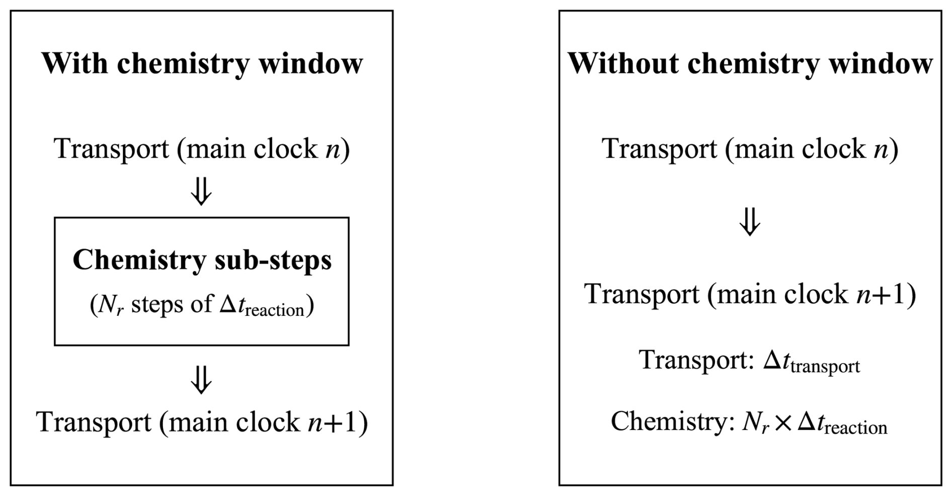
Although the dual-clock scheme allows chemical reactions to evolve on finer internal sub-steps, it also introduces synchronisation issues. Extremely small transport steps are required to capture fast kinetics, which may offset the intended efficiency gain, whereas overly large sub-steps can reduce temporal resolution and cause numerical errors. Nevertheless, this framework is well suited for problems where the transport and reaction processes operate on distinct time scales, and the chemical feedback is relatively weak, providing an effective balance between accuracy and computational efficiency.

3.2 Integration strategy

The overall integration workflow is illustrated in Fig. 2. At the start of the simulation, PhreeqcRM performs an initialisation stage that reads the configuration parameters, loads the prescribed geochemical conditions, and computes the initial aqueous-element concentrations and mineral-phase abundances. In coordination with OpenFOAM, these initial values are mapped onto the computational mesh so that each control volume is assigned its starting aqueous and mineral concentrations. These fields serve as the baseline for subsequent transport and reaction calculations.

Figure 2 Numerical simulation procedure for present model.

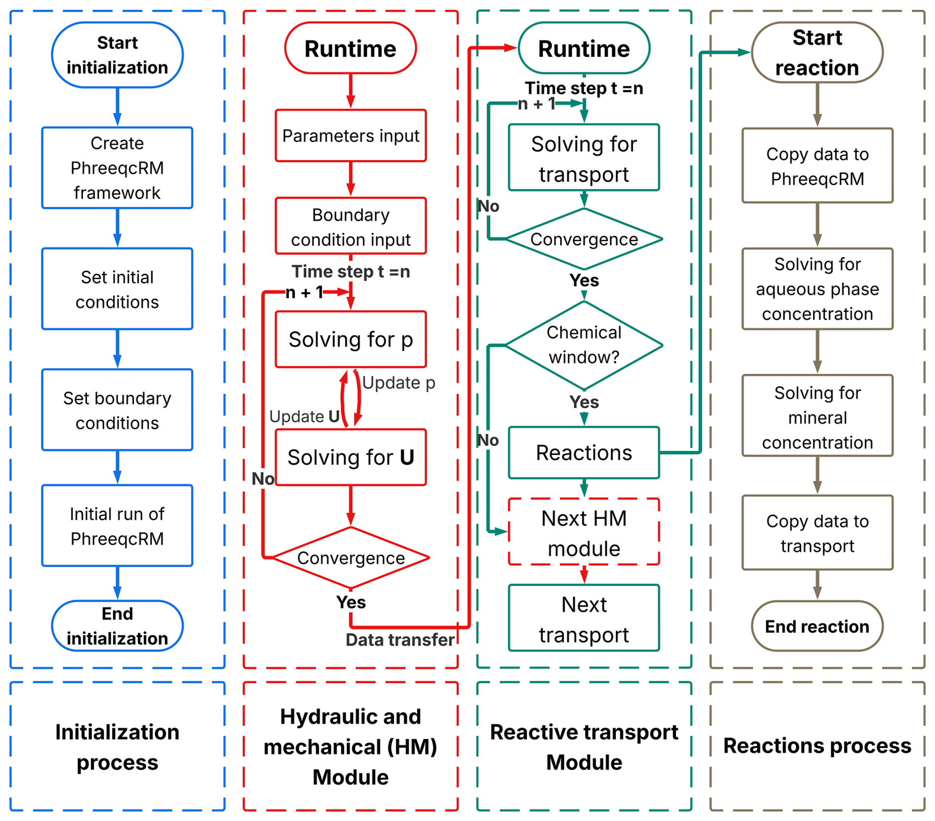
For each global time step thereafter, OpenFOAM first solves the hydro-mechanical (HM) subsystem, pore pressure, mechanical deformation, and elemental advection–dispersion transport. Although the flow and deformation equations are strongly coupled through the pore-pressure–displacement interaction, solving them in a fully monolithic manner is numerically demanding and often computationally expensive. To improve robustness and efficiency, the present framework adopts a segregated iterative strategy, which has been widely used in CFD. The pressure equation is solved first using the previous iteration's displacement field. The resulting pressure distribution is then used to update the solid skeleton deformation, and only explicit terms are refreshed at each iteration. This process repeats until the change between successive iterations falls below a prescribed tolerance, at which point convergence is declared. The convergent fields of pore pressure p and displacement u_s are then passed in a one-way manner to the transport module to define the pore-fluid velocity v_f and solid velocity v_s required by the advection–dispersion equation for solute migration.

After the HM and transport updates, the solver checks whether the current simulation time falls within the user-defined reaction-activation window. If the chemical module is inactive, the solver skips the reaction step and proceeds directly to the next global time step. If the chemical module is active, OpenFOAM first assembles the elemental concentration fields from all computational cells into a contiguous vector conforming to the data structure required by PhreeqcRM. This vector is passed to PhreeqcRM, which performs aqueous speciation and kinetic-reaction calculations to update both aqueous concentrations and mineral-phase abundances. Upon completion, PhreeqcRM overwrites the same vector with the updated results, which are then mapped back into the OpenFOAM fields of each cell. The simulation proceeds to the next global HM–transport step using these updated concentrations.

3.3 Numerical stability

Within the OpenFOAM framework adopted in this study, the governing equations were discretised using the finite volume method. Diffusive and dispersive fluxes were evaluated using the Gauss linear scheme, while the advective term of solute transport was discretised using a Gauss limitedLinear scheme with a limiter coefficient of 1 in order to suppress spurious oscillations. Temporal integration was performed using the implicit Euler method. The pressure, displacement and concentration equations were solved using the GAMG solver with a DILU preconditioner, with absolute and relative tolerances of 10⁻⁹ and zero, respectively. The coupled HMC system was advanced using a segregated outer-iteration strategy, and convergence was achieved when the residuals of all primary variables dropped below 10⁻⁶. Further implementation details are provided in the companion paper (Wang and Jeng, 2025).

To strengthen the numerical credibility of the proposed HMC framework, a systematic sensitivity analysis was conducted with respect to spatial discretisation, global time-step size and chemical sub-stepping in the ChemWindow controller. A one-at-a-time strategy was adopted, whereby only one numerical factor was varied while all others were kept identical.

The numerical deviations were quantified using the mean relative error (MRE) and maximum relative error (MaxRE), defined as

$$\begin{array}{}\text{(11)}& \mathrm{\text{MRE}}={\displaystyle \frac{\mathrm{1}}{N}}\sum _{i=\mathrm{1}}^N\left|{\displaystyle \frac{y_i-y_i^{\mathrm{ref}}}{y_i^{\mathrm{ref}}}}\right|,\text{MaxRE}=\underset{\mathrm{1}\le i\le N}{max}\left|{\displaystyle \frac{y_i-y_i^{\mathrm{ref}}}{y_i^{\mathrm{ref}}}}\right|,\end{array}$$

where y_i denotes the computed value at the ith comparison point and $y_i^{\mathrm{ref}}$ is the corresponding value obtained from the finest reference solution. The MRE reflects the overall deviation level, whereas the MaxRE captures the largest local discrepancy associated with potential non-linear or synchronisation effects.

The reference configuration corresponds to the finest grid (120 × 1 × 100), the smallest global time step (Δt = 1.58 ×10⁵ s), and the smallest chemical sub-step (Δt_c = 3000 s). The medium discretisation employs a grid of 60 × 1 × 50 with $\mathrm{\Delta }t=\mathrm{3.15}\times {\mathrm{10}}^{\mathrm{5}}\mathrm{s}$ and Δt_c = 6000 s, while the coarse setting uses 30 × 1 × 25, Δt = 6.31 × 10⁵ s, and Δt_c = 12 000 s.

Table 1 together with Figs. 3 and 4 summarises the grid-, time-step- and chemical-substep-independence results for pore pressure p, solid displacement u_s and solute concentration Y.C. For the hydro-mechanical variables p and u_s, both the MRE and MaxRE decrease rapidly with mesh refinement and global time-step reduction. In all medium–fine comparisons, the maximum relative errors remain below 0.5 %, indicating excellent numerical convergence of the hydro-mechanical part of the solver.

Table 1 Grid-, time-step-, and chemical-substep-independence summary.

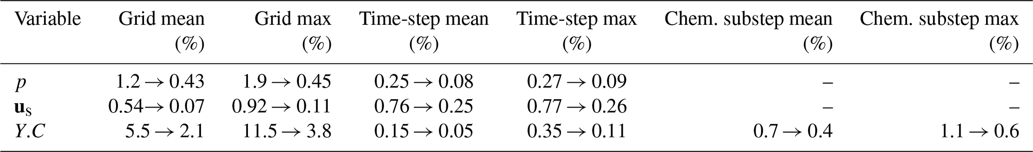
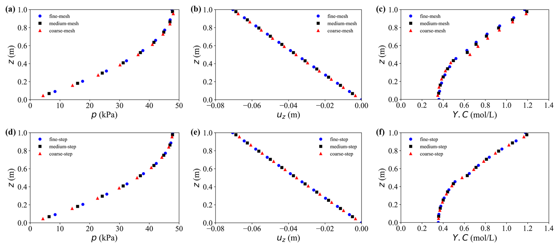
Figure 3 Grid and time step independence analysis. (a–c) Results under different grid resolutions: (a) pore water pressure, (b) vertical displacement, and (c) solute concentration. (d–f) Results under different time step sizes: (d) pore water pressure, (e) vertical displacement, and (f) solute concentration.

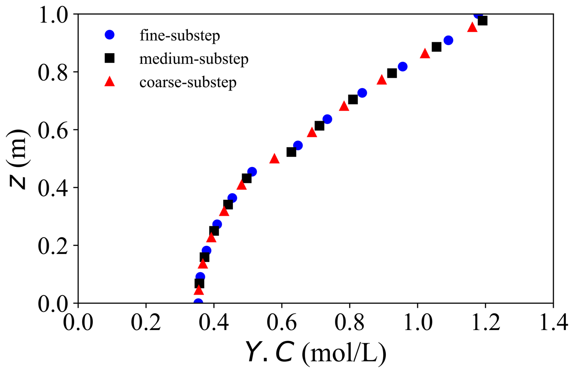
Figure 4 Analysis of chemical-substep independence: small substep (round), medium substep (square), large substep (triangle).

The solute concentration Y.C exhibits a higher sensitivity to spatial resolution, as expected for advection–dispersion–reaction dominated processes. Nevertheless, the MaxRE decreases from 11.5 % in the coarse–fine comparison to 3.8 % in the medium–fine comparison, while the MRE reduces from 5.5 % to 2.1 %, demonstrating satisfactory convergence of the transport component. In contrast, the sensitivity to the global time-step size is negligible, with maximum discrepancies below 0.2 %. More importantly, decreasing the chemical sub-step size from 12 000 to 3000 s results in less than 1 % variation in solute concentration, with the MaxRE reducing from 1.1 % to 0.6 %. This confirms that the proposed ChemWindow synchronisation scheme is numerically stable and does not introduce artificial splitting errors.

Based on these results, the medium discretisation settings (60 × 1 × 50, Δt = 3.15 × 10⁵ s, Δt_c = 6000 s) are adopted in the remainder of this study as a balanced compromise between numerical accuracy and computational efficiency.

3.4 Verification with previous studies

Two benchmark problems were used to verify different components of the present model and to examine the numerical stability of the solvers. Laboratory data is not available in the literature for direct comparison. However, benchmarking against published numerical results is a well‐established practice in the field of reactive solute transport, and provides a practical means to confirm model implementation before applying it to new scenarios.

3.4.1 Verification No. 1: Hydro–mechanical–transport (without reactions)

The first benchmark was designed to validate the hydro–mechanical–transport (HM–T) module implemented in OpenFOAM, with chemical reactions excluded. All material properties, boundary conditions, and loading settings were kept identical to those reported by Wu and Jeng (2023), who solved the same problem using the commercial package COMSOL.

The dissipation of the simulated pore pressure and vertical displacement show excellent agreement with Wu and Jeng (2023) in the domain and in all reported directions, confirming the precision of the coupled flow–deformation implementation (Fig. 5). A minor early-time deviation appears in the breakthrough concentration at the model top. A plausible cause for this discrepancy is the difference in dimensional treatment between the two codes: COMSOL solves a strictly planar (two-dimensional (2-D)) problem, whereas OpenFOAM emulates 2-D by extruding a thin 3-D slab.

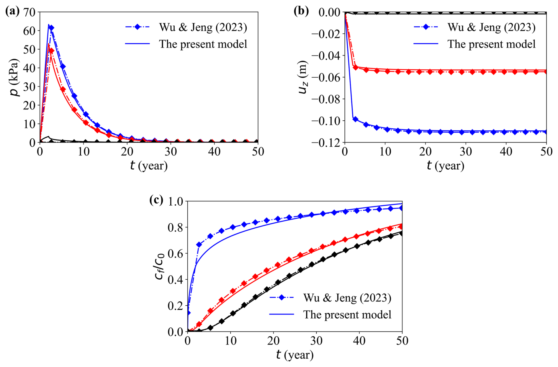
Figure 5 Comparison between the present model and previous model (Wu and Jeng, 2023). Temporal evolution of (a) pore water pressure, (b) vertical displacement, and (c) normalised solute concentration $C_f/C_{\mathrm{0}}$. Lines represent different depths: top (blue), middle (red), and bottom (black).

This quasi-2-D setup introduces several non-ideal effects: (i) the finite out-of-plane thickness implies a small but non-zero storage capacity, which can alter the volumetric flux per unit width; (ii) the high-aspect-ratio cells in the thin direction tends to increase the numerical (and possibly physical) transverse dispersion, which slightly smears the sharp concentration front; (iii) differences in boundary treatment for the thin direction (e.g., empty vs. symmetryPlane) and related gradient corrections can produce small phase shifts in the concentration profile.

3.4.2 Verification No. 2: Reactive solute transport with kinetic dissolution

The second benchmark was designed to evaluate the OpenFOAM–PhreeqcRM coupling for simulating kinetically controlled mineral reactions under advective–dispersive transport. In this test, the HM module was disabled and a constant velocity of 1 × 10⁻⁴ m³ s⁻¹ (volumetric injection rate) was imposed. The solid matrix comprised 57 % inert mineral and 3 % calcite, while an acid solution of pH = 2 was continuously injected, following the configuration reported by Pavuluri et al. (2022) (also implemented in OpenFOAM). A one-dimensional (1-D) transport domain was used to represent calcite dissolution and precipitation during migration. The simulated concentration profiles of dissolved Ca were compared with those reported in the reference study, as shown in Fig. 6. Overall, the two solutions exhibit good agreement at intermediate and late times, whereas noticeable discrepancies arise during the early breakthrough stage.

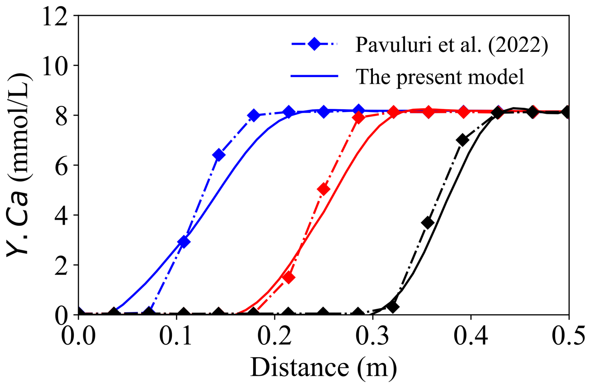
Figure 6 Comparison of the present model (solid line) with Benchmark 2 (Pavuluri et al., 2022, diamond markers). The blue line represents the result at 20 min, the red line at 40 min, and the black line at 60 min.

The discrepancies observed between the two solutions are primarily attributed to the fundamentally different discrete treatments of the advective transport term, which lead to distinct boundary flux reconstructions. The reference solver evaluates the advective operator using the surface-based volumetric flux field ϕ in the form ∇⋅(ϕY_i), whereas the present framework formulates advection in terms of the divergence of a Darcy-based, cell-centred mass flux, ∇⋅(v_fY_i). Owing to the distinct surface-flux and volume-flux formulations, the two operators are not discretely equivalent.

Consequently, even when identical fixedValue boundary conditions are prescribed, the resulting advective fluxes differ in the discrete implementation, because ϕ is imposed directly at cell faces, while v_f is defined at cell centres and subsequently interpolated to the boundary faces. This structural difference cannot be expected to vanish systematically through mesh refinement and therefore gives rise to irreducible discrepancies during the early transient stage.

Within this context, Benchmark #2 is not intended to provide strict equation-to-equation validation against the reference solution, but rather to assess the correctness and feasibility of the proposed governing equations under comparable conditions. The observed agreement in the overall trend and magnitude of the concentration profiles supports the correctness of the present implementation and indicates that the proposed control equations capture the dominant dissolution dynamics. The remaining differences are mainly attributable to the distinct discrete treatments of the advective operator.

4 Application to a landfill liner

The developed framework is designed to simulate coupled flow, deformation and multicomponent reactive transport in porous media subjected simultaneously to mechanical loading and chemically aggressive fluids. This modelling tool is broadly applicable to scenarios where barrier materials interact with reactive solutes, for example, chloride ingress that accelerates steel corrosion in reinforced concrete structures (Guo et al., 2024), or advective–dispersive transport through clay liners accompanied by cation exchange and carbonate dissolution or precipitation (Guo and Na, 2023).

In this study, the framework is applied to a landfill-liner scenario. Chemically aggressive leachates, such as acidic solutions enriched in CO${}_{\mathrm{3}}^{-}$, SO${}_{\mathrm{4}}^{\mathrm{2}-}$, can infiltrate the liner and react with both its mineral constituents and the underlying geomaterials, thus improving contaminant migration and potentially compromising the long-term performance of the barrier.

4.1 Model description

In OpenFOAM, a quasi-2-D domain (Fig. 7) was built as a thin 3-D slab of length L_x = 20 m and height L_z = 1 m, with a negligible out-of-plane thickness to emulate two-dimensional behaviour. Along the top boundary, three contaminant inlets (depicted by blue arrows) are prescribed as boundary molar fluxes J₁–J₃ with units of mol (m² s)⁻¹. Each inlet is applied uniformly over a top-boundary patch of width 4 m (i.e., an inlet area A_i = 4 m × 0.02 m, where 0.02 m is the out-of-plane thickness of the quasi-2-D OpenFOAM model). The intervening top-boundary segments are assigned zero solute flux. The entire top surface is subjected to a uniform mechanical load. The bottom boundary comprises five localised drainage outlets (red arrows) with a prescribed hydraulic head, with the rest rendered impermeable; both lateral boundaries are also impermeable and mechanically fixed to prevent rigid body motion.

Figure 7 Cross section of the present model.

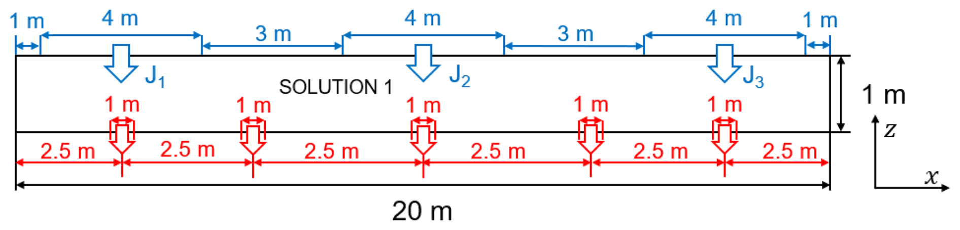
The coordinate system is defined such that x is positive to the right and z is positive upward. The geochemical initial condition is spatially uniform: the entire computational domain is assigned Solution 1 from the PHREEQC input file, thus providing the same initial aqueous composition throughout the liner and the surrounding geomaterial. Each OpenFOAM cell is directly mapped to a corresponding PHREEQC cell, ensuring a one-to-one correspondence between the flow and geochemical grids. If spatially variable initial compositions are required (i.e., different Solution definitions), the OpenFOAM mesh must be preconfigured to assign the appropriate PHREEQC solution number to each computational cell.

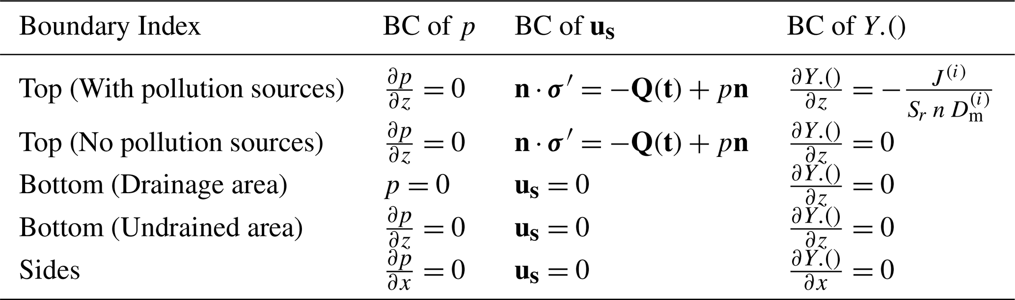
4.2 Boundary conditions and input parameters

A mechanical load is applied at the top boundary and expressed through the local force-balance condition.

$$\begin{array}{}\text{(12)}& -\mathbf{n}\cdot {\mathit{\sigma }}^{\prime }=\mathbf{Q}\left(t\right)-\mathbf{n}\cdot p\mathbf{I},\end{array}$$

where n is the outward unit normal, σ^′ denotes the effective stress tensor, and I is the identity tensor. The effective stress is defined following Jasak and Weller (2000), and the corresponding displacement gradient on the loaded surface is given by

$$\begin{array}{}\text{(13)}& \begin{array}{rl}& \mathbf{n}\cdot \mathrm{\nabla }{\mathbf{u}}_{\mathbf{s}}\\ & ={\displaystyle \frac{-\mathbf{Q}\left(t\right)-\left[\mathbf{n}\cdot \mathit{\mu }{\left(\mathrm{\nabla }{\mathbf{u}}_{\mathbf{s}}\right)}^T+\mathit{\lambda }\mathbf{I}\mathrm{tr}\left(\mathrm{\nabla }{\mathbf{u}}_{\mathbf{s}}\right)-(\mathit{\mu }+\mathit{\lambda })\mathrm{\nabla }{\mathbf{u}}_{\mathbf{s}}\right]+\mathbf{n}p}{\mathrm{2}\mathit{\mu }+\mathit{\lambda }}}.\end{array}\end{array}$$

The bottom boundary is constrained to emulate a stiff foundation: both vertical and lateral components of displacement are fixed at zero, suppressing downward settlement and horizontal sliding along the base. The lateral boundaries are laterally fixed to prevent rigid-body motion of the entire domain, but their vertical displacement remains free unless otherwise specified.

For pore pressure, the top surface is assumed to be in contact with an overlying ponded leachate at atmospheric pressure and is therefore assigned a zero normal gradient condition,

$$\begin{array}{}\text{(14)}& {\displaystyle \frac{\partial p(x,y,\mathrm{0},t)}{\partial z}}=\mathrm{0},\end{array}$$

which is consistent with a flat free surface in static equilibrium and negligible vertical seepage. Under near-saturated conditions, the liquid phase remains continuous up to the surface while the gas phase is disconnected, so no capillary head or hydrostatic jump develops across the interface. If a sustained head difference develops between the ponded leachate and the liner interior, a non-zero gradient or a Dirichlet-type pressure specification would be required to represent advective inflow.

The lateral boundaries are treated as impermeable for flow, enforcing no-drainage (zero-normal-flux) conditions. At the bottom boundary, drainage is permitted only at the designated outlet segments where hydraulic head is prescribed, while the remaining sections of the bottom share the same no-drainage condition as the lateral boundaries.

The boundary of solute concentration at the top is specified as

$$\begin{array}{}\text{(15)}& {\displaystyle \frac{\partial Y.(x,y,\mathrm{0},t)}{\partial z}}=-{\displaystyle \frac{J^{\left(i\right)}}{S_{r}n{D}_{\mathrm{m}}^{\left(i\right)}}},\end{array}$$

where J⁽ⁱ⁾ the imposed vertical solute-mass flux of elements i, and $D_{\mathrm{m}}^{\left(i\right)}$ the molecular diffusion coefficient. This Robin-type, diffusion-controlled boundary is appropriate when the overlying leachate pond has negligible vertical seepage yet maintains a concentration gradient that drives diffusive mass transfer into the liner. If appreciable advective inflow occurs, a prescribed advective flux or a Dirichlet-type concentration boundary would be more suitable. The lateral boundaries and the impermeable portions of the bottom boundary are assigned zero normal gradient (Neumann) conditions for concentration. The boundary conditions are summarised in Table 2.

Table 2 Boundary conditions (BCs) setup for the present models.

It is emphasised that the imposed concentration boundary conditions are adopted as controlled demonstration settings to explore the sensitivity of coupled hydro-mechanical–chemical responses to source strength and drainage configuration. The leakage cases considered correspond to localised defects or preferential pathways rather than spatially uniform barrier failure, which is not regarded as realistic for engineered containment systems. In the absence of site-specific investigation data, the present simulations should therefore be interpreted as scenario-based analyses aimed at mechanistic understanding, rather than predictive landfill exposure assessments.

The simulated liner is modelled as a low permeability clayey soil under a small-strain linear elastic framework (Table 3). Hydraulic and mechanical properties—including porosity n, degree of saturation S_r, hydraulic conductivity K, shear modulus G, Poisson's ratio ν, and compressibility coefficients—were taken from representative ranges for compacted clay liners (Peters and Smith, 2002; Zhang et al., 2012). These values are consistent with the small-strain assumption, allowing the use of linear elasticity and the Eulerian formulation without large-deformation corrections. Geochemical reactions are implemented via the PhreeqcRM interface, in which standard PHREEQC input blocks are specified using OpenFOAM chemistry dictionaries. Details of the corresponding configuration options are provided in Appendix D.

For reactive-transport simulations, the linear distribution coefficient K_d, a simplified equilibrium sorption term, was set to zero for all elements so that changes in breakthrough and spatial distribution arise solely from geochemical reactions such as mineral dissolution and precipitation. The PHREEQC reaction module is, in principle, capable of representing more complex sorption mechanisms (e.g. nonlinear Freundlich or Langmuir isotherms and competitive or kinetic adsorption–desorption), but these functionalities are reserved for future extensions and are not used in this work.

Table 3 Physical parameters of the present models.

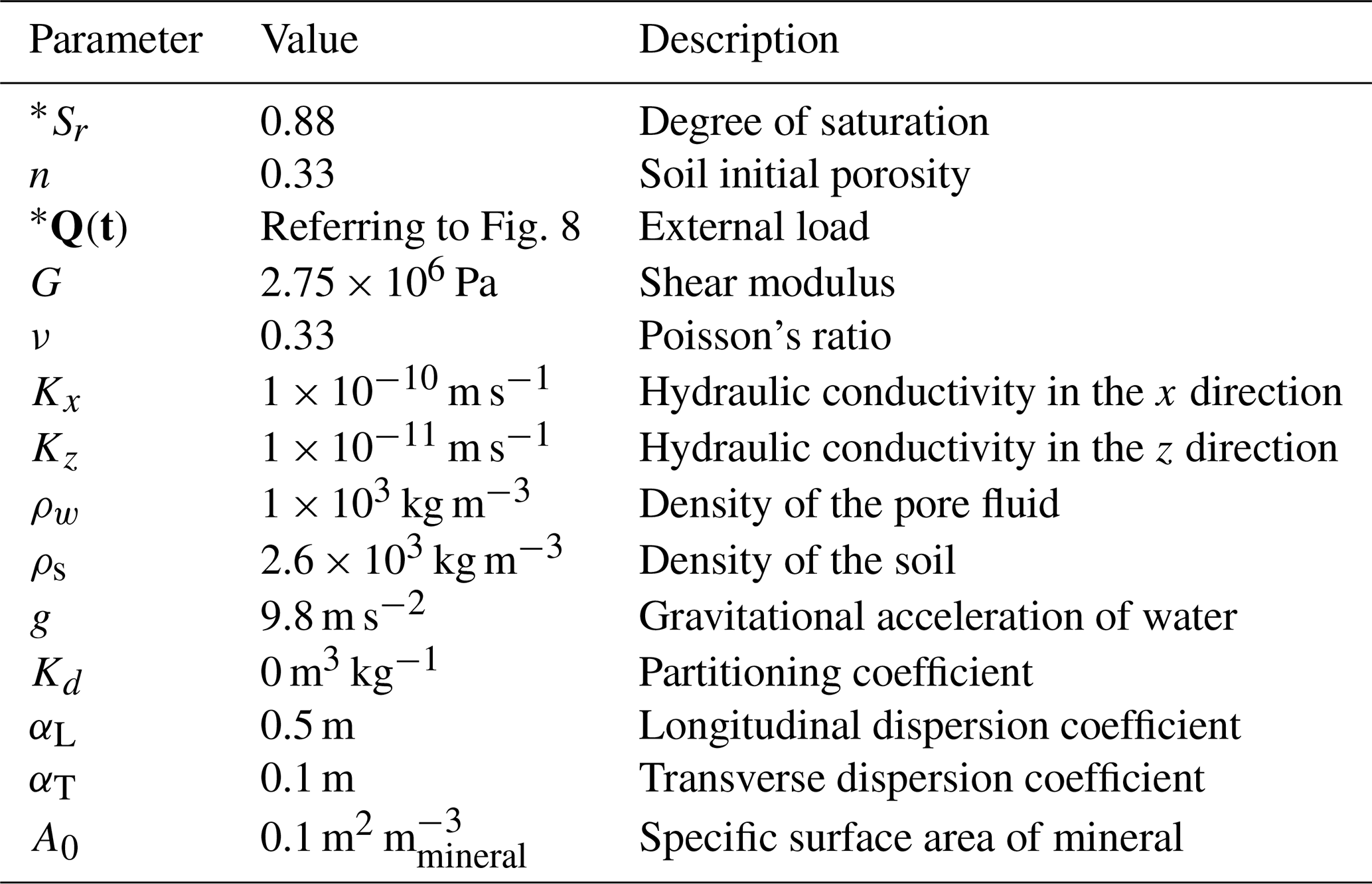
Note: parameters with ^* were used in the parametric study.

4.3 Description of case studies

Two types of reactive‐transport scenarios were designed to demonstrate and evaluate the capabilities of the proposed HMC framework. The first case considers a single reactive mineral that undergoes multicomponent aqueous reactions, enabling a clear examination of the fundamental coupling between hydro-mechanical processes and geochemical reaction fronts. This case is also used to explore the sensitivity of the system response to external mechanical loading and to variations in the initial degree of saturation, highlighting the interaction between pore pressure dissipation, deformation, and reactive solute migration.

The second case extends the system to a multi‐mineral, multi‐component reaction network to showcase the stability of the framework to capture simultaneous dissolution–precipitation and competitive aqueous reactions among several solid phases. This progression from a simplified to a more complex geochemical setting highlights the versatility of the solver and its ability to handle general reactive transport problems.

4.3.1 Single mineral reaction

The dissolution and precipitation of calcite in the CO₂–water system follow the classical carbonate reaction,

$$\begin{array}{}\text{(16)}& {\mathrm{CaCO}}_{\mathrm{3}}\left(\mathrm{s}\right)+{\mathrm{CO}}_{\mathrm{2}}\left(\mathrm{aq}\right)+{\mathrm{H}}_{\mathrm{2}}\mathrm{O}\left(\mathrm{l}\right)\rightleftharpoons {\mathrm{Ca}}^{\mathrm{2}+}\left(\mathrm{aq}\right)+\mathrm{2}{\mathrm{HCO}}_{\mathrm{3}}^{-}\left(\mathrm{aq}\right),\end{array}$$

which describes the equilibrium between solid calcite, dissolved CO₂, and bicarbonate species.

Rather than assuming instantaneous equilibrium, calcite dissolution and precipitation were represented using the surface-controlled kinetic law (Plummer et al., 1978):

$$\begin{array}{}\text{(17)}& \begin{array}{rl}& r_{\mathrm{v}}\left(t\right)\\ & =A_{\mathrm{eff}}\left(M\right)\left[k_{\mathrm{1}}\right(T)a_{{\mathrm{H}}^{+}}+k_{\mathrm{2}}(T)a_{{\mathrm{H}}_{\mathrm{2}}{\mathrm{CO}}_{\mathrm{3}}^{*}}+k_{\mathrm{3}}(T\left)a_{{\mathrm{H}}_{\mathrm{2}}\mathrm{O}}\right]\\ & (\mathrm{1}-{\mathrm{10}}^{\mathit{\eta }{\text{SI}}_{\mathrm{calcite}}}),\end{array}\end{array}$$

where r_v(t) is the volumetric rate of reaction (mol m${}_{\mathrm{bulk}}^{-\mathrm{3}}$ s⁻¹); $A_{\mathrm{eff}}\left(M\right)=A_{\mathrm{0}}(M/M_{\mathrm{0}}{)}^m$ is the effective reactive surface area that scales with the remaining mineral mass M; k₁, k₂, and k₃ are temperature-dependent rate constants representing the acid (H⁺), carbonic-acid (H₂CO${}_{\mathrm{3}}^{*}$), and neutral (H₂O) mechanisms, respectively; a_i denotes the activity of aqueous species i; SI_calcite is the saturation index controlling the departure from equilibrium (SI < 0 favours dissolution, SI > 0 favours precipitation); η is an empirical coefficient (typically η ≈ 1), and m is the surface-area scaling exponent (commonly m = 2/3).

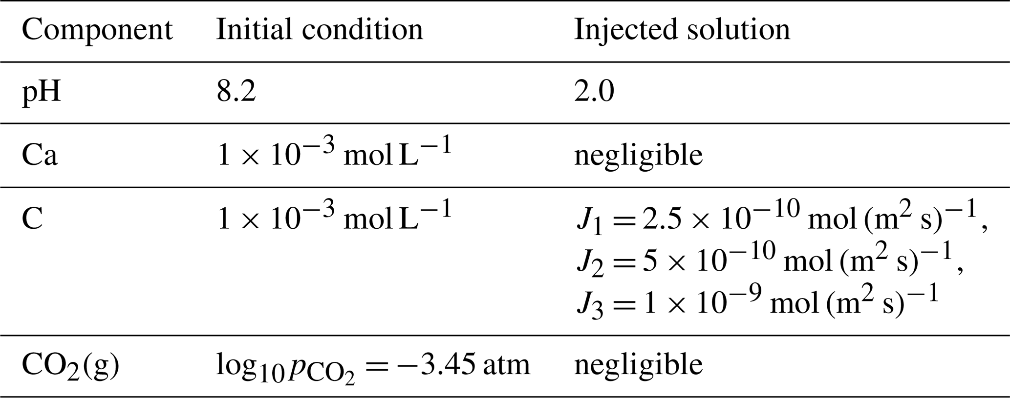
Table 4 lists the primary chemical components of the background pore water and the injected acidic solution. The porous medium initially contained 57 % inert mineral and 3 % calcite. The background water was near-neutral, CO₂-buffered, and close to calcite saturation, while the injected solution was strongly acidic (pH = 2). Acidic inflow reduced the local calcite saturation index, promoting calcite dissolution and releasing Ca²⁺ and HCO${}_{\mathrm{3}}^{-}$ into the aqueous phase. The solute fluxes imposed for inorganic carbon differed between the three injection points, designated J₁, J₂ and J₃ as shown in Fig. 7. These sources are located in the left, middle, and right sections of the upper boundary, respectively, with the injection strength progressively increasing from J₁ to J₃.

Table 4 Primary components in the background (initial) and injected solutions for the single-mineral reaction.

To examine the effects of hydro–mechanical coupling, external loading, and saturation on reactive solute migration, three groups of simulation scenarios were designed:

• 1.

  Group 1: Mechanistic influence (Cases A–C)

  • -

    Case A: Baseline full HMC coupling (hydro–mechanical coupling, solute transport, and chemical reactions); vertical load 4.0 × 10⁵ Pa applied for two years at S_r=0.88.

  • -

    Case B: Same as Case A, but with geochemical reactions deactivated (no-chem).

  • -

    Case C: Same as Case A, but with the mechanical module removed (no-mech; reactive transport only).

• 2.

  Group 2: Load sensitivity (Cases D–E) (Fig. 8)

  • -

    Case D: Higher vertical load 6.0 × 10⁵ Pa, other settings as in Case A (HMC).

  • -

    Case E: Lower vertical load 2.0 × 10⁵ Pa, other settings as in Case A (HMC).

• 3.

  Group 3: Saturation sensitivity and module exclusion (Cases F–K)

  • -

    Case F: HMC at S_r=1.0 (other settings as in Case A).

  • -

    Case G: HMC at S_r=0.80 (other settings as in Case A).

  • -

    Case H: No-mech (RT+Chem) at S_r=1.0 (same as Case F but without mechanics).

  • -

    Case I: No-mech (RT+Chem) at S_r=0.80 (same as Case G but without mechanics).

  • -

    Case J: No-chem (HM+T) at S_r=1.0 (same as Case F but without geochemical reactions).

  • -

    Case K: No-chem (HM+T) at S_r=0.80 (same as Case G but without geochemical reactions).

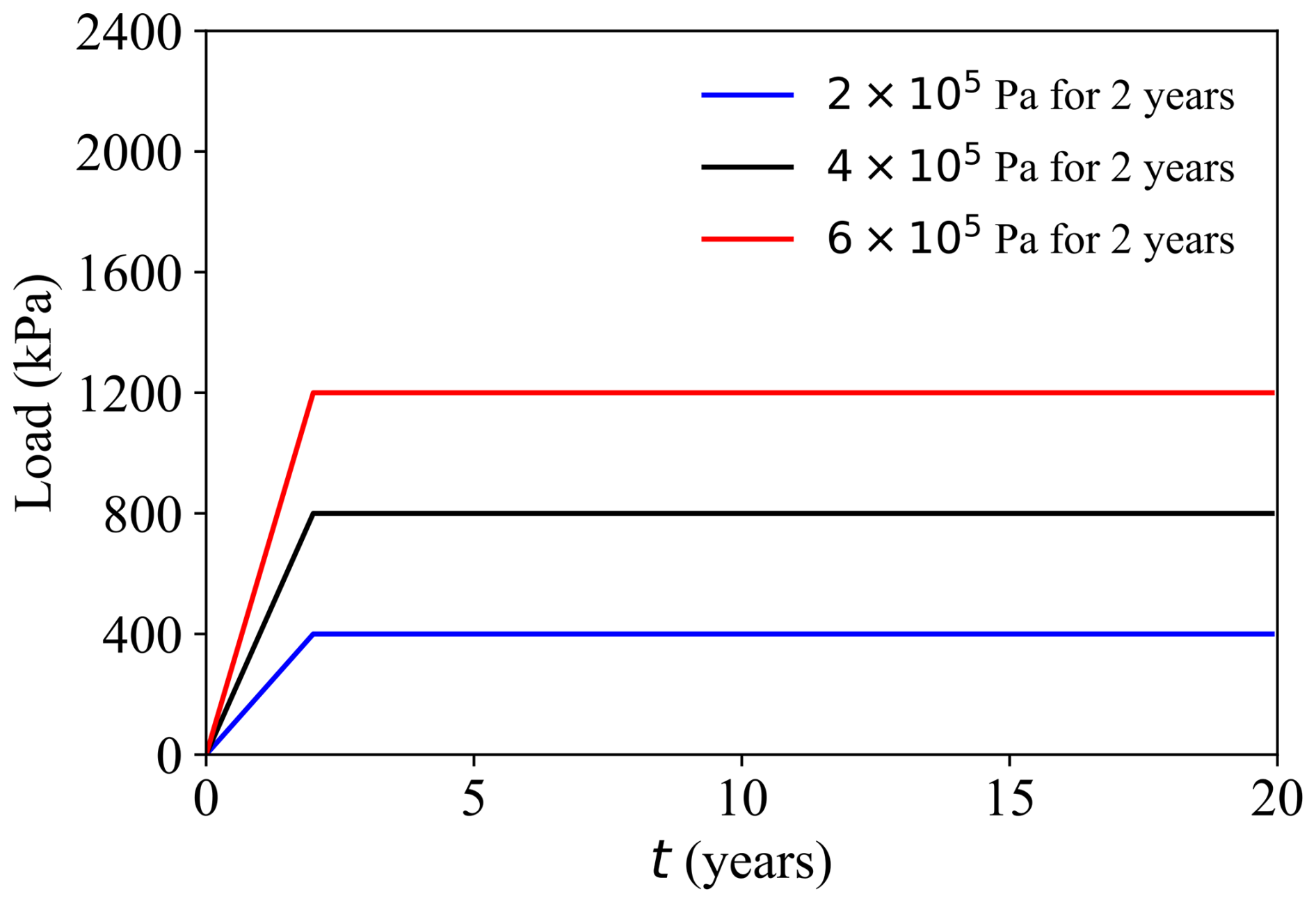
Figure 8 Load pattern under different models: the black line represents Case A, the red line represents Case D, and the blue line represents Case E.

4.3.2 Multi-mineral reaction

The simulations also consider two additional reactive minerals in Model L: gibbsite (Al(OH)₃) and siderite (FeCO₃), whose dissolution–precipitation reactions in aqueous systems are

$$\begin{array}{}\text{(18)}& {\displaystyle }\mathrm{Al}\left(\mathrm{OH}{)}_{\mathrm{3}}\right(\mathrm{s})+\mathrm{3}{\mathrm{H}}^{+}\left(\mathrm{aq}\right)\rightleftharpoons {\mathrm{Al}}^{\mathrm{3}+}\left(\mathrm{aq}\right)+\mathrm{3}{\mathrm{H}}_{\mathrm{2}}\mathrm{O}\left(\mathrm{l}\right),\text{(19)}& {\displaystyle }{\mathrm{FeCO}}_{\mathrm{3}}\left(\mathrm{s}\right)+{\mathrm{H}}^{+}\left(\mathrm{aq}\right)\rightleftharpoons {\mathrm{Fe}}^{\mathrm{2}+}\left(\mathrm{aq}\right)+{\mathrm{HCO}}_{\mathrm{3}}^{-}\left(\mathrm{aq}\right),\end{array}$$

Both minerals were treated as non-equilibrium phases whose dissolution or precipitation follows a surface-area–controlled kinetic law:

$$\begin{array}{}\text{(20)}& r_{A,j}\left(t\right)=k_j\left(T\right)(\mathrm{1}-{\mathrm{10}}^{{\mathit{\eta }}_j{\text{SI}}_j}),j\in \mathit{\left\{}\text{Gibbsite,\hspace{0.17em}Siderite}\mathit{\right\}},\end{array}$$

where r_A,j is the areal rate (mol m⁻² s⁻¹), k_j(T) is a temperature-dependent rate constant (e.g. $k_{\mathrm{gibbsite}}=\mathrm{5}\times {\mathrm{10}}^{-\mathrm{10}}$ and $k_{\mathrm{siderite}}=\mathrm{5}\times {\mathrm{10}}^{-\mathrm{9}}$ mol m⁻² s⁻¹ in the implementation of PHREEQC at 25 °C), SI_j is the saturation index of the mineral j and η_j is an empirical coefficient (typically η_j ≈ 1).

Table 5 summarises the multi-mineral scenario, which represents an acidic and oxidising plume injected into a near-neutral, CO₂-buffered carbonate aquifer. The aquifer initially contained calcite (22 %), gibbsite (5 %), siderite (5 %), and an inert mineral (33 %). The injected plume, characterised by low pH and continuous inflow of C, Fe, and Al, interacted with near-neutral background groundwater and altered its pH and redox state. These chemical perturbations could dissolve or precipitate the resident carbonate and hydroxide minerals, depending on the degree of mixing between the injected plume and the background pore water.

Table 5 Primary components in the background (initial) and injected solutions for the multi-mineral reaction.

5 Numerical results and discussion

This section presents numerical simulations for landfill liner scenarios and highlights the key physical insights from coupled hydromechanical-chemical (HMC) analyses. Section 5.1 examines how deformation combined with chemical reactions affects pore pressure dissipation, solute migration, and mineral alteration, and compares the system responses under different external loads. Section 5.2 evaluates how changes in the initial degree of saturation modify the coupled hydro-mechanical–chemical behaviour. Section 5.3 investigates the role of multiple reactive minerals in shaping the evolution of concentration and the advancement of reaction fronts. Section 5.4 discusses the trade-off between model accuracy and computational cost, providing guidance on the practical usability of the model.

5.1 Effect of external load and chemical reactions on solute migration

This subsection investigates how external loading and aqueous reactions jointly influence solute migration and calcite dissolution by varying the magnitude of loading, deformation behaviour, and dissolution-reaction pathways.

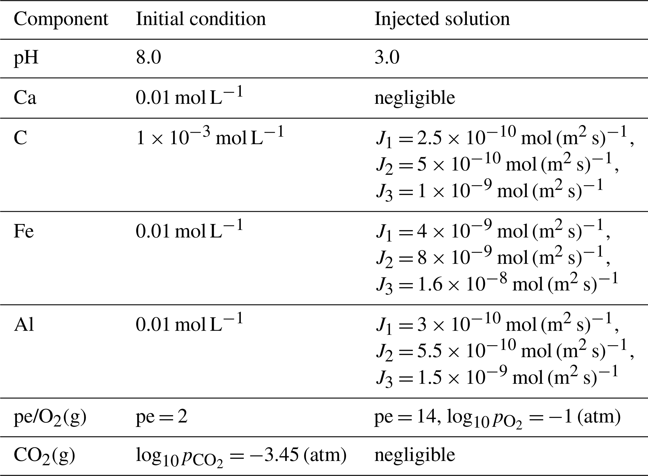
Under bottom drainage conditions, all three loading cases demonstrate that a higher load produces a larger initial pore-water pressure, slower dissipation, and greater ultimate settlement (Fig. 9a, b). A larger initial excess pressure requires a longer time to dissipate, thus extending the deformation period despite a greater absolute pressure drop. At mid-depth (z = 0.5 m), which is closer to the drainage outlet, the pore pressure dissipates more rapidly and the displacement stabilises earlier. Overall, Case D exhibits the highest pore pressure response and settlement, followed by Case A and then Case E, confirming that increasing load amplifies both pressure evolution and deformation.

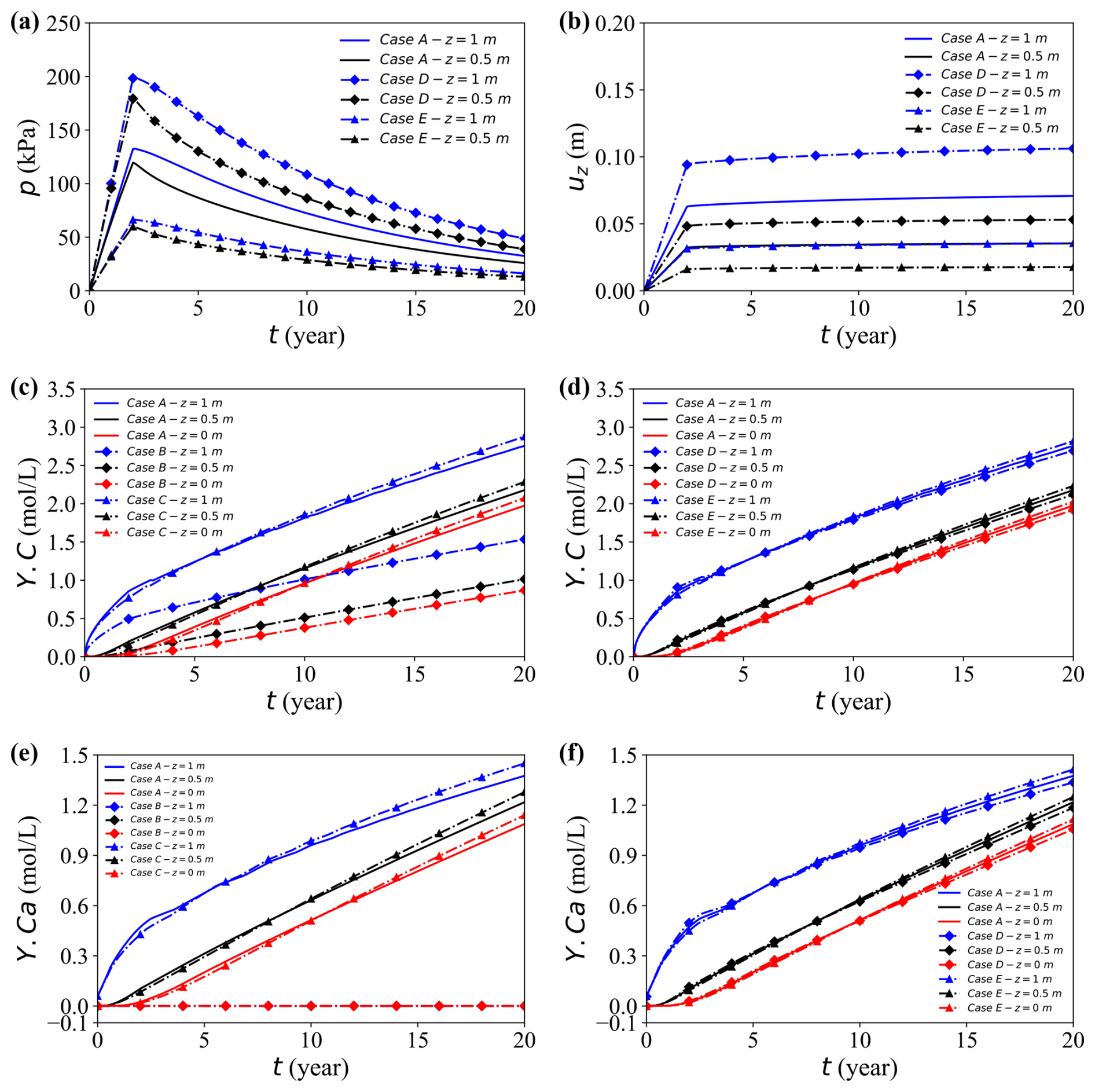
Figure 9 Temporal evolution of the coupled responses at the observation point (x = 17 m) for different cases. (a, b) Pore water pressure and vertical displacement for Cases A, D, and E. (c, d) Concentration Y.C for Cases A–C and A, D, and E, respectively. (e, f) Concentration Y.Ca for Cases A–C and A, D, and E, respectively.

Figure 9c–h illustrate the temporal evolution of aqueous concentrations within the calcite-dissolution system under different mechanistic scenarios. In Fig. 9c (elemental carbon), Case B – which excludes aqueous reactions – yields markedly lower concentrations than the other cases because chemical reactions are suppressed. Case C, where matrix deformation is neglected, exhibits a crossover behaviour: its concentration is lower than that of the fully coupled Case A at early times but becomes higher at later stages. This reversal arises because deformation during consolidation reduces the pore volume and flow ability, thereby restricting early advective release of dissolved species. In contrast, the absence of deformation preserves pore connectivity and facilitates solute transport, resulting in higher late-time concentrations.

The influence of mechanical compression is further highlighted under varying loading magnitudes (Fig. 9d). Initially, higher loads accelerate the release of the solute through increased flow and reduction of porosity, but as compression progresses, the decrease in pore volume and flow ability restrict later stage transport. Consequently, long-term concentrations under heavy loads become lower than those observed under lighter loads.

Unlike Y.C, Y.Ca has no external solute source, the initial calcium concentration is negligible and increases only by calcite dissolution. Accordingly, Fig. 9e shows a gradual increase in aqueous Ca²⁺ over time, while Case B remains essentially zero because no calcium derived from dissolution is supplied. Figure 9e–f further demonstrate that higher loads or the inclusion of deformation compress the soil skeleton, reducing porosity and flow capacity. These mechanical changes alter the transport pathways and influence the rate at which calcium accumulates, underscoring the coupled role of stress, deformation, and chemical reactions in governing long-term redistribution of solutes.

Figures 10 and 11 present 2-D contour maps at t = 20 years for dissolved carbon (Y.C) originating from calcite dissolution (Fig. 10) and calcium (Y.Ca) released by the same process (Fig. 11). Three external source zones are clearly visible, with strengths increasing from left to right. This gradient produces markedly different peak concentrations across the sources – for instance, under Case A, the rightmost source exhibits approximately two to three times higher concentrations than the leftmost one.

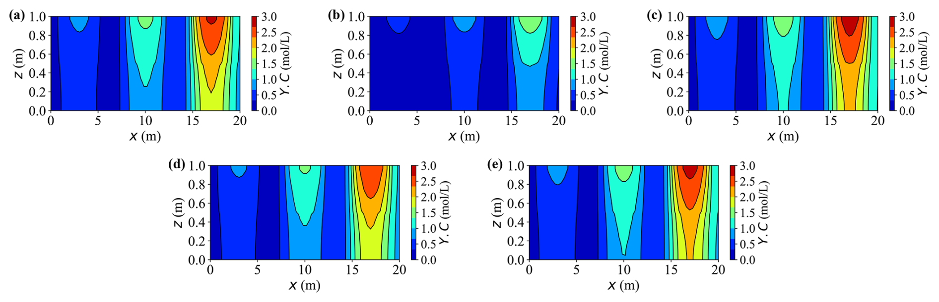
Figure 10 Contour plots of concentration Y.C at t = 20 years for different cases. (a–e) Results for Cases A–E, respectively.

Figure 11 Contour plots of concentration Y.Ca at t = 20 years for different cases. (a–e) Results for Cases A–E, respectively.

In Fig. 10, the carbon concentration field follows a similar spatial pattern, reaffirming that neglecting deformation or applying a smaller load accelerates dissolution and enhances solute accumulation. The three distinct source-controlled peaks along the horizontal direction are clearly delineated. Initially, the migration of the solute occurs predominantly in the vertical direction following the main drainage pathway, and with time, it spreads laterally. These maps confirm that the mechanisms identified in the temporal profiles, specifically the effects of deformation, loading magnitude, and reaction coupling, also govern horizontal solute dispersion.

In Fig. 11, the calcium concentration fields exhibit trends consistent with the earlier time series results, now extending into a full spatial perspective. The transition from vertical to horizontal migration highlights preferential transport pathways shaped by loading and deformation. As expected, Case B remains near zero because there is no dissolution-reaction source, while the other cases display distinct high concentration regions aligned with the three source zones. Enhanced mechanical compression hinders fluid migration and solute dispersion, leading to narrower plumes and lower concentration peaks than in lighter-load or un-deformed cases such as Cases C and E.

Figure 12 shows the two-dimensional contour maps of pH at t = 20 years. The pH distribution closely mirrors the dissolved carbon and calcium fields, being primarily governed by local ionic equilibria within the aqueous phase. Zones enriched in dissolved calcium and carbonate species exhibit lower pH (more acidic), while areas with limited accumulation of solutes remain near the background weakly acidic level (pH ≈ 6.5–7.0). Accordingly, cases or source zones that generate higher solute concentrations develop broader and deeper low pH regions, while non-reactive regions maintain near-neutral conditions.

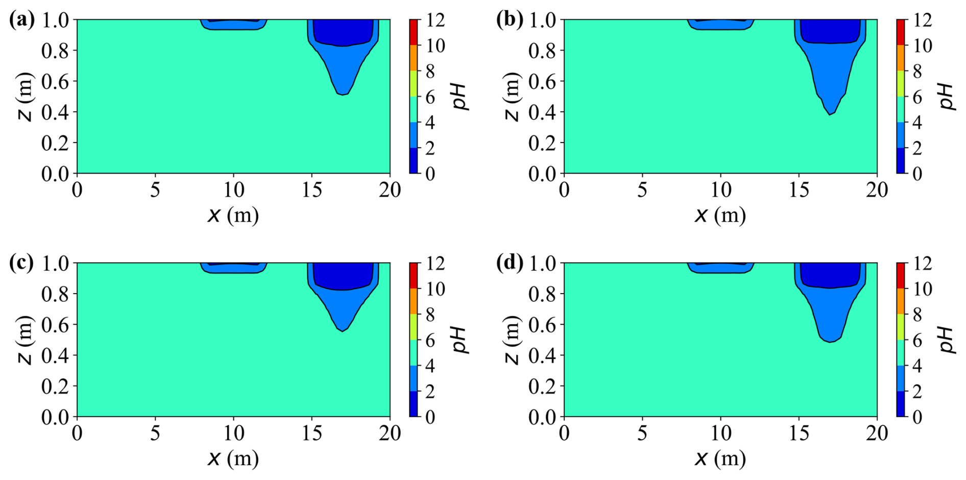
Figure 12 Spatial distribution of pH at t = 20 years for different cases. (a–d) Results for Cases A, C, D, and E, respectively.

Figure 13 presents two-dimensional contour maps of calcite dissolution at different times. During the early stage (up to approximately 10 years), dissolution remains concentrated beneath the strongest sources of contaminants. In Case A, the upper layer below the rightmost source, where the inflow is strongest, loses nearly 15 % of its initial calcite mass by year 10, whereas the depletion beneath the weakest leftmost source remains below 5 %.

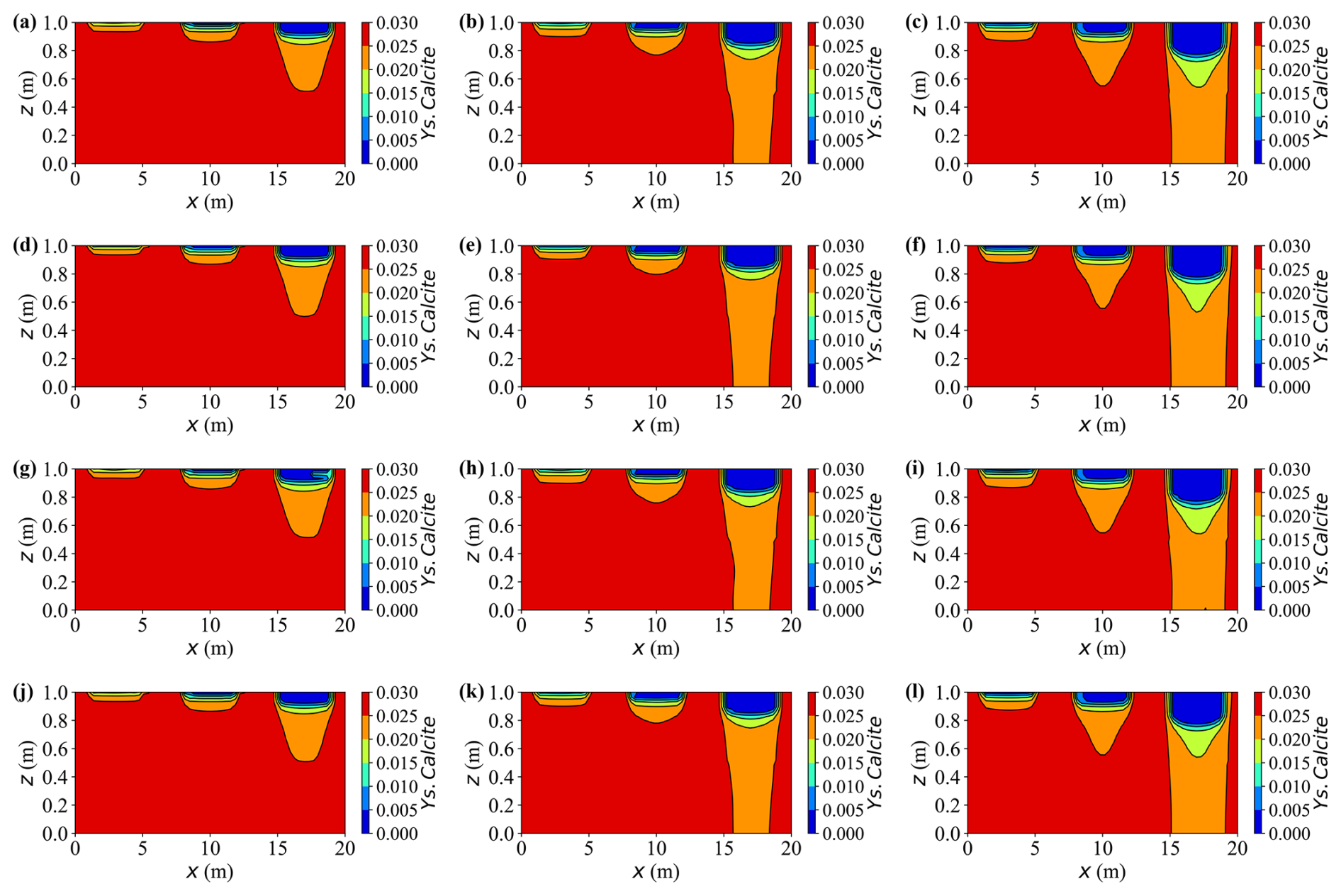
Figure 13 Spatial distribution of Ys.Calcite content at different times for various cases. (a–c) Case A at t = 10, 15, and 20 years, respectively; (d–f) Case C at t = 10, 15, and 20 years, respectively; (g–i) Case D at t = 10, 15, and 20 years, respectively; (j–l) Case E at t = 10, 15, and 20 years, respectively.

The results reveal that external loading exerts a pronounced influence on the morphology and evolution of the reactive front. With increasing load, the transition between the reacted and unreacted zones becomes progressively smoother and more diffuse, while in the non-deforming case (Case C) it remains narrow and sharply defined. For example, at t = 20 years, the front thickness measured as the horizontal distance of 40 % calcite-depletion isolines—widens from approximately 1.4 m in Case C to 2 m under high load (Case A). Consistently, the 2-D maps of aqueous concentration confirm this behaviour: the concentration front is distinctly sharper in the non-deforming case (Case C), whereas deformation produces a smoother and more diffuse transition across the reactive zone.

This “mechanical smoothing effect” arises from differences in solute distribution and local chemical disequilibrium. Under higher external load, pore pressure redistribution alters the concentration field, redirecting solute transport predominantly along the horizontal direction rather than vertically. As a result, the dissolved products (e.g. Ca²⁺, HCO${}_{\mathrm{3}}^{-}$) spread laterally and accumulate near the reaction zone, moderating vertical concentration gradients and producing a more diffuse dissolution front. This accumulation increases the local saturation index (SI_calcite) and reduces the thermodynamic driving force term (1−10^n SI), thus slowing and broadening the dissolution process spatially. Consequently, concentration gradients across the front are gradually smoothed, yielding a wider, more diffuse reactive zone. In contrast, the non-deforming case (Case C) maintains stronger undersaturation and steeper concentration gradients, resulting in a sharper, advection-controlled interface that propagates more abruptly through the matrix.

Together, these results demonstrate that dissolution, flow-driven transport, and load-induced pore-space evolution jointly control the timing and magnitude of solute concentrations. The 2-D contour maps corroborate the line-based profiles, confirming that these trends persist in the horizontal direction and revealing peak differences and lateral plume structures, such as spreading and source-zone interactions, not captured by 1-D analyses.

5.2 Effect of saturation on reactive transport

This subsection examines how saturation conditions influence reactive solute transport in deformable porous media. Figure 14a and b compare excess pore pressure p and vertical displacement u_z between three representative cases: the near-saturated baseline Case A (S_r = 0.88), the fully saturated Case F (S_r = 1.0), and the less-saturated Case G (S_r = 0.80). The mechanical response strongly depends on the saturation. The fully saturated Case F exhibits the highest excess pore pressure – approximately 400 kPa at the top, nearly three times that of Case G – because its pores are filled with nearly incompressible water that resists volumetric change under load.

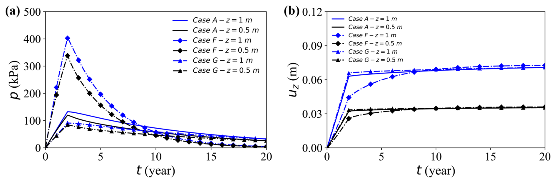
Figure 14 Temporal evolution of pore water pressure and vertical displacement at the observation point (x = 17 m) for selected cases. (a, b) Results for Cases A, F, and G.

Although all cases reach similar final surface settlements (≈ 0.065 m), Case F requires substantially longer to stabilise, as excess pressure dissipates only through slow water drainage in the absence of compressible gas. Lower saturation reduces both the pore water content and the initial pressure peak, facilitating faster dissipation and earlier stabilisation; Case G, for instance, shows roughly 45 % lower peak p and settles much earlier than Case F.

Figure 15a–e depict the spatial and temporal evolution of dissolved calcium (Y.Ca) and carbon (Y.C) at different saturation levels. Both solutes exhibit similar behaviour: lower saturation generally enhances aqueous concentrations. Comparison in the three case groups (Fig. 15c–e) clarifies the distinct and combined functions of deformation, saturation, and geochemical reactions.

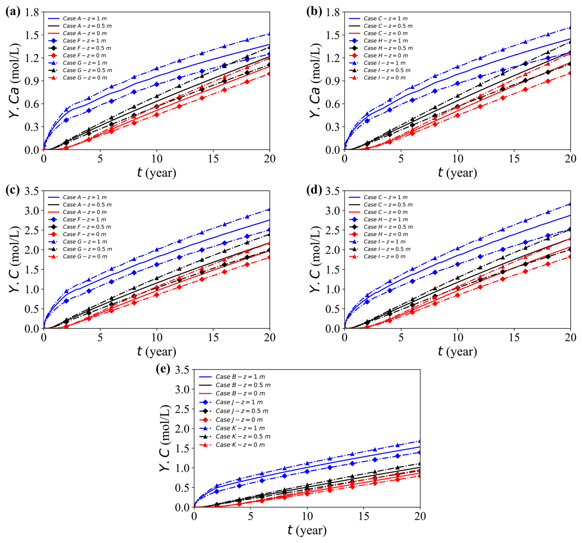
Figure 15 Temporal evolution of solute concentrations at the observation point (x = 17 m) for different cases. (a, b) Concentration Y.Ca for Cases A, F, and G, and Cases C, H, and I, respectively. (c, d) Concentration Y.C for Cases A, F, and G, and Cases C, H, and I, respectively. (e) Concentration Y.C for Cases B, J, and K.

The Case B, J, and K group disables geochemical reactions to isolate the influence of mechanical deformation. Although total compression is nearly identical in all cases, the drainage rate varies markedly with saturation. In fully saturated condition, excess pore pressure slowly dissipates and the resulting limited fluid mobility restricts advective transport, leading to lower solute concentrations. In contrast, partially saturated conditions allow faster drainage and stronger advection, which promote vertical redistribution. Thus, the observed concentration difference primarily reflects drainage-controlled advection capacity rather than differences in overall deformation magnitude.

In contrast, the Case C, H, I group suppresses deformation but retains geochemical reactions, thus isolating the reaction-driven response to varying saturation. Here, decreasing S_r elevates the concentrations mainly because the available water volume (θ_w = nS_r) diminishes; thus, the same mass of the dissolution-derived solute is distributed into a smaller liquid volume, producing uniformly higher aqueous concentrations. This $\mathrm{1}/{\mathit{\theta }}_{\mathrm{w}}$ scaling amplifies the contrast between saturation levels.

Finally, the Case A, F, G group activates both deformation and geochemical reactions, and the observed patterns reflect their combined influence. Geochemical processes increase the levels of solutes through ongoing dissolution, while lower saturation further magnifies these increases by reducing the aqueous volume. Meanwhile, mechanical compression partially counteracts this enhancement by reducing the level of pore connectivity and limiting the degree of advective redistribution. In general, geochemical reactions amplify saturation-driven contrasts, whereas mechanical deformation provides a modest damping effect on solute concentrations under any given saturation.

Figures 16a–i present the two-dimensional distributions of dissolved carbon (Y.C) at t = 20 years for all case groups. Compared with earlier vertical profiles, these maps emphasise the pronounced horizontal variability shaped by the three contaminant sources. Peak concentrations consistently occur near the rightmost source where the inflow is strongest, reaching Y.C ≈ 3.0 mol L⁻¹, approximately two to three times higher than those near the weakest leftmost source. Horizontal plumes are progressively broadened from right to left, revealing distinct source–plume separation and limited mixing between adjacent zones.

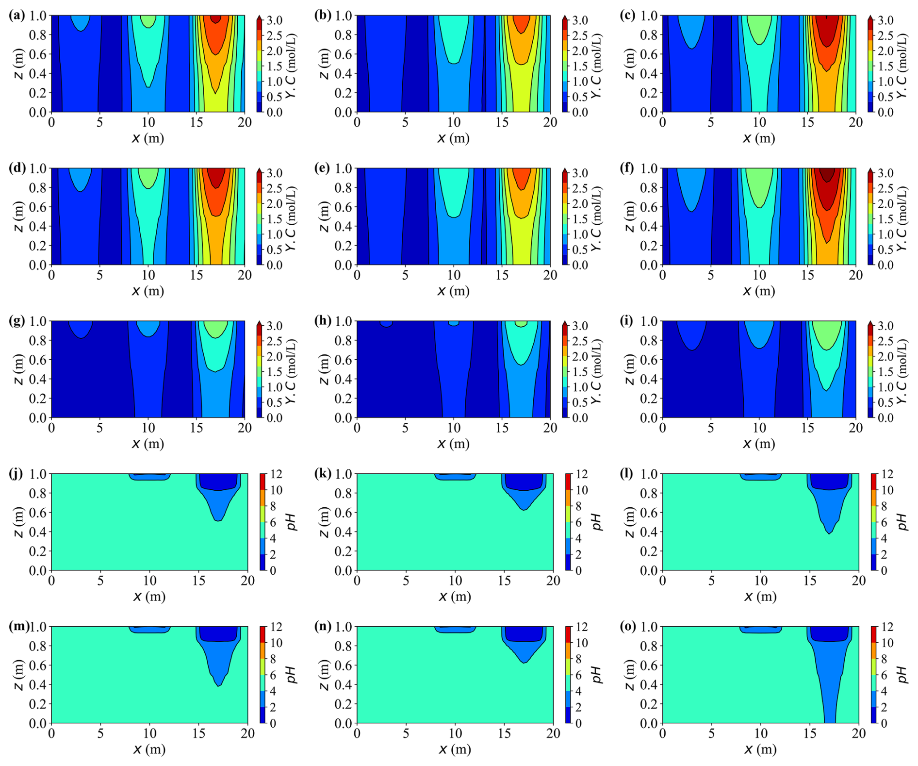
Figure 16 Spatial distributions of concentration Y.C and pH at t = 20 years for different cases. Panels (a)–(c), (d)–(f), and (g)–(i) show Y.C for Cases A, F, and G; C, H, and I; and B, J, and K, respectively. Panels (j)–(l) and (m)–(o) show pH for Cases A, F, and G and cases C, H, and I, respectively.

Lower saturation elevates aqueous concentrations throughout the domain, particularly around the strong right-hand source, where the high-solute cores expand laterally by about 15 %–20 % in Case G relative to Case F. Similar conclusions can be drawn from Cases J and K. In contrast, mechanical deformation exerts an opposing influence: at the same saturation level, the peak Y.C values in deformable cases (e.g., Case G versus Case I) are about 20 % lower, and the corresponding high-concentration plumes appear more confined and compact.

The pH distributions (Fig. 16j–o) reflect the coupled influence of dissolved calcium, carbonate species, and other ions on local aqueous equilibria. Regions with higher solute concentrations develop broader and more acidic zones, while areas with limited solute accumulation remain close to neutral. Consequently, the extent of acidification closely mirrors both the intensity and lateral extent of the solute plumes.

Overall, the results indicate that saturation variations exert a stronger control on chemical concentrations and plume geometry than on the final mechanical deformation. Although saturation influences response magnitudes, the governing mechanisms and comparative trends remain consistent across S_r 0.8–1.0. Lower saturation amplifies both the magnitude and the horizontal reach of high-concentration plumes, while mechanical deformation slightly suppresses the concentration peaks and contracts the plume footprints. Together, these trends highlight the competing effects of saturation and deformation on the long-term spread of reactive solutes in deformable porous media.

5.3 An example of multi-mineral reaction

The purpose of this subsection is to demonstrate the capability of the developed solver to handle multi-component and multi-mineral reactions, thus establishing a foundational framework for future model extensions.

Figures 17 and 18 illustrate the temporal evolution of aqueous chemistry and mineral reactions driven by three externally supplied contaminants, carbon (Y.C), iron (Y.Fe), and aluminium (Y.Al), with source intensities decreasing from left to right. Among the three, the external influx of iron is the strongest, followed by aluminium, while carbon has the weakest source. However, the retained aqueous concentrations show the opposite order (C > Fe > Al) due to their distinct reaction pathways. Dissolved carbon maintains the highest residual level, with typical peaks around 6.6 mol L⁻¹, while dissolved iron and aluminium reach lower quasi-steady concentrations of approximately 0.2 mol L⁻¹ and 0.12 mol L⁻¹, respectively. Aluminium undergoes the most intensive reaction: the introduced Al³⁺ rapidly precipitates as gibbsite (Al(OH)₃), leaving only trace amounts of dissolved aluminium in the aqueous phase. As a result, the aluminium plume appears nearly stationary, giving the impression of limited solute migration despite strong local reactions.

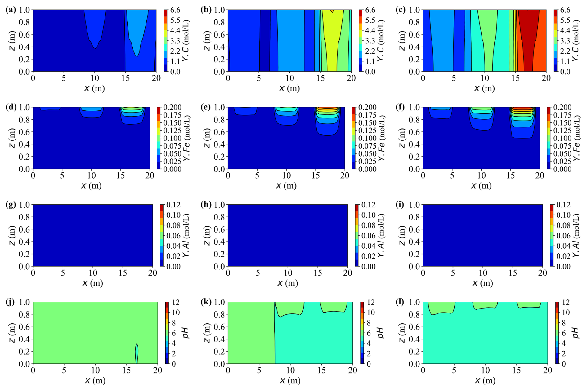
Figure 17 Spatial distributions of aqueous concentrations and pH at different times for Case L. (a–c) Concentration of Y.C at t = 10, 30, and 50 years, respectively. (d–f) Concentration of Y.Fe at t = 10, 30, and 50 years, respectively. (g–i) Concentration of Y.Al at t = 10, 30, and 50 years, respectively. (j–l) pH at t = 10, 30, and 50 years, respectively.

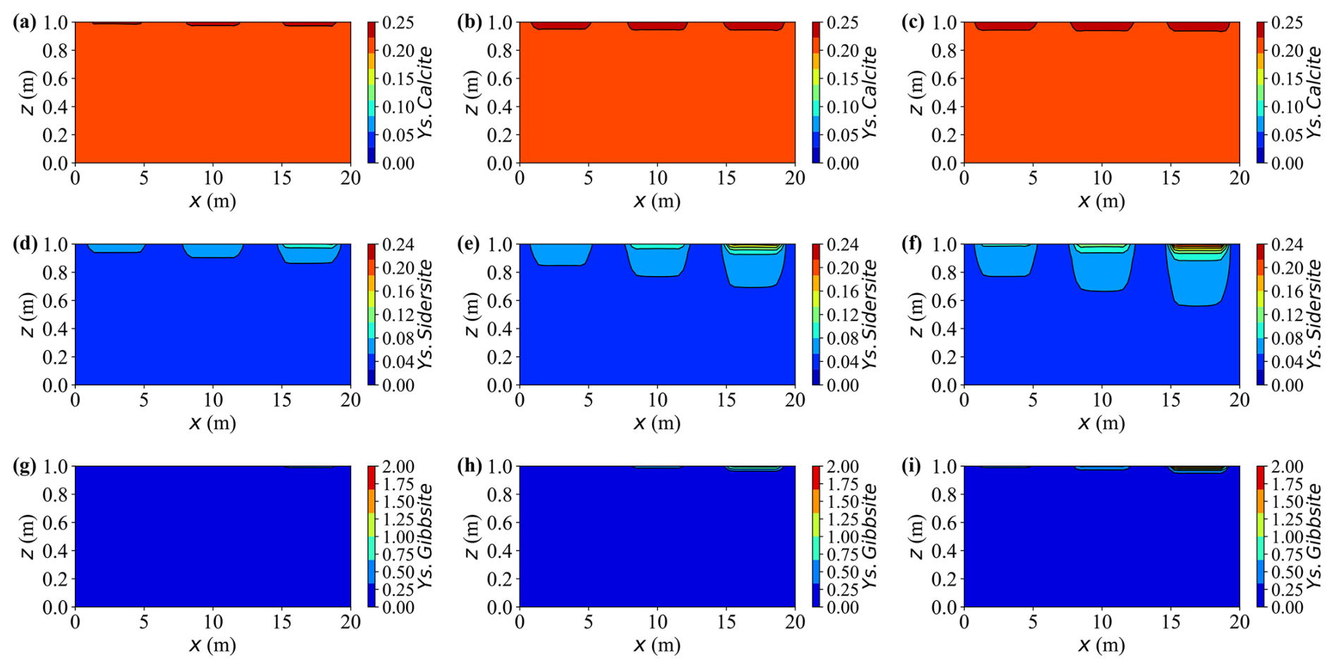
Figure 18 Spatial distributions of mineral contents at different times for Case L. (a–c) Ys.Calcite content at t = 10, 30, and 50 years, respectively. (d–f) Ys.Sidersite content at t = 10, 30, and 50 years, respectively. (g–i) Ys.Gibbsite content at t = 10, 30, and 50 years, respectively.

Initially, the injected source solution is mildly alkaline due to the presence of hydroxyl- and carbonate-bearing complexes such as Al(OH)${}_{\mathrm{4}}^{-}$ and HCO${}_{\mathrm{3}}^{-}$. As reactions proceed, the precipitation of gibbsite (Al(OH)₃) and siderite (FeCO₃) releases protons through hydrolysis and carbonate exchange, progressively neutralising the alkalinity and driving the system towards mildly acidic conditions. Calcite (CaCO₃) also precipitates, but plays a dual role by partially buffering the acidity generated through its dissolution equilibrium. Spatially, the right-hand side exhibits a faster pH decline than the left-hand side, primarily because of stronger precipitation reactions and weaker carbonate buffering in that region.

Calcite remains persistently oversaturated throughout the simulation, indicating a continuous but slow precipitation. This sluggish behaviour arises from two limiting factors: low concentration Ca²⁺ and a mildly acidic environment (pH ≈ 6.0). Under such conditions, most dissolved inorganic carbon (DIC) exists as HCO${}_{\mathrm{3}}^{-}$ rather than CO${}_{\mathrm{3}}^{\mathrm{2}-}$, thus reducing the effective carbonate activity required for calcite growth. Consequently, net calcite precipitation proceeds slowly, achieving only a modest increase of about 15 % of its initial mass by year 50. Although the process consumes small amounts of Ca²⁺ and bicarbonate ions, the resulting buffering capacity is insufficient to neutralise the protons released from metal hydrolysis and gibbsite formation. Hence, calcite acts as a slow but persistent secondary precipitate phase under calcium- and pH-limited conditions.

Siderite forms at a moderate but sustained rate where injected Fe²⁺ overlaps with carbonate species supplied by the carbon source (Y.C, primarily HCO${}_{\mathrm{3}}^{-}$ $/$ CO${}_{\mathrm{3}}^{\mathrm{2}-}$). Concomitant precipitation of calcite competes for carbonate and thus moderates siderite growth. Compared with gibbsite, the siderite front advances more slowly and extends over a broader region. By year 30, siderite captures roughly 25 %–30 % of the incoming iron along the primary flow paths, increasing to approximately 40 %–45 % by year 50. As a result, dissolved iron concentrations peak near the source, governed by the source strength, and gradually attenuate downstream under reaction control.

Upon arrival of Y.Al, gibbsite precipitates rapidly, causing an abrupt decrease in the dissolved aluminium near the source. Quantitatively, more than 80 % of the incoming Al is removed within the first 10 years in the proximal zone, and the cumulative fraction increases from approximately 5 % initially to nearly 20 % by year 50. Because the precipitation rate greatly exceeds the advective transport rate, most reactions remain confined to the source region, leaving negligible aluminium migration downstream. This behaviour characterises a strongly reaction-controlled regime, where rapid local precipitation suppresses long-range solute propagation.

In general, the solver consistently reproduces these coupled processes: progressive plume expansion over 10–50 years, clear dependence on source strength, moderated pH evolution, and mass-conserving behaviour across all solutes. These results confirm that the model robustly simulates complex, multi-mineral reactive transport involving concurrent precipitation and dissolution fronts.

5.4 Computational performance

All simulations were performed on a workstation equipped with an Intel Xeon Silver 4114 CPU (2.20 GHz) and 256 GB RAM. Unless otherwise specified, each case was solved using four parallel MPI processes under the same hardware configuration to ensure consistency and fair comparison of CPU time and memory usage.

To evaluate numerical efficiency and assess the trade-off between computational cost and accuracy, this subsection compares the performance of the full HMC solver with its simplified counterparts, in which either the chemical module is deactivated. The evaluation considers four key indicators: total CPU time, average time per step, maximum RAM usage, and the relative error of solute concentration at the most responsive monitoring point. For each paired comparison, the fully coupled HMC case under identical loading and saturation conditions (Cases A, F, G) serves as the reference, while the simplified (Cases B, K) and multi-mineral (Case L) cases are evaluated against it.

The relative error (RE_Q(%)) quantifies the deviation of a simplified model from its corresponding full HMC reference under the same loading and saturation. For a time-dependent variable Q(t) (e.g., carbon concentration Y.C) measured at a monitoring point, RE_Q(%) is defined using the L²-norm of the temporal series, normalised by the reference:

$$\begin{array}{}\text{(21)}& {\text{RE}}_Q\left(\mathit{\%}\right)={\displaystyle \frac{{∥Q_{\mathrm{model}}\left(t\right)-Q_{\mathrm{HMC},\mathrm{ref}}\left(t\right)∥}_{L^{\mathrm{2}}(\mathrm{0},T)}}{{∥Q_{\mathrm{HMC},\mathrm{ref}}\left(t\right)∥}_{L^{\mathrm{2}}(\mathrm{0},T)}}}\times \mathrm{100},\end{array}$$

where $\Vert X{\Vert }_{L^{\mathrm{2}}(\mathrm{0},T)}$ = $\sqrt{{\int }_{\mathrm{0}}^T{X}^{\mathrm{2}}\left(t\right)\mathrm{d}t}$. In this study, RE_Q(%) is evaluated at the most responsive monitoring point identified from the HMC baseline for each comparison.

Table 6 summarises the computational cost and relative error evaluated at the top monitoring point (x = 17 m, z = 1 m). All reported performance metrics correspond to the output of the first MPI process (rank 0). Complete HMC simulations (A, F, G) required approximately 25–26 h of CPU time, while deactivation of chemical reactions (B, J, K) reduced total runtime by more than two orders of magnitude, with almost identical memory consumption. The nearly constant use of RAM arises because all cases share the same mesh and field allocations; enabling a module does not significantly alter the solver's data structure or storage requirements. However, this simplification introduces substantial concentration deviations (RE_c ≈ 44 %), demonstrating the importance of retaining chemical coupling to capture realistic solute behaviour. In contrast, the multi-mineral reactive case (L) exhibited the highest computational demand, reflecting the increased cost associated with solving the extended reaction network. Overall, these results confirm that while simplified configurations offer significant computational savings, they do so at the expense of accuracy, underscoring the necessity of HMC modelling for quantitative predictive analyses.

Table 6 Computational cost and relative error at the top responsive point (x = 17 m, z = 1 m).

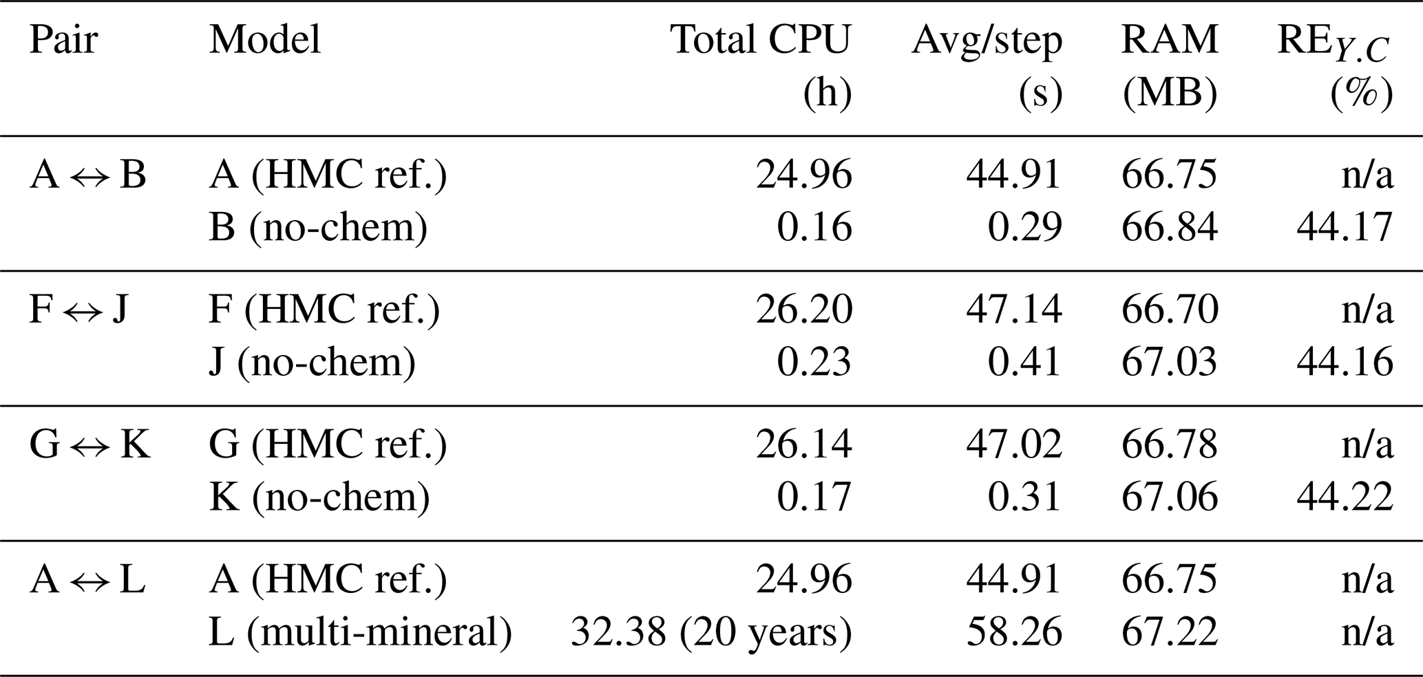
Notes: CPU times measured on the same hardware. RAM = maximum resident set size. n/a: not applicable.

To evaluate the parallel efficiency of the developed solver, the wall time required for a 5-year simulation is analysed as a function of the number of MPI processes. Figure 19 presents the measured wall time together with the corresponding speedup, which is defined relative to the baseline case with two MPI processes as Speedup = $T_{\mathrm{2}}/T_N$.

Figure 19 Wall time and speedup versus number of MPI processes.

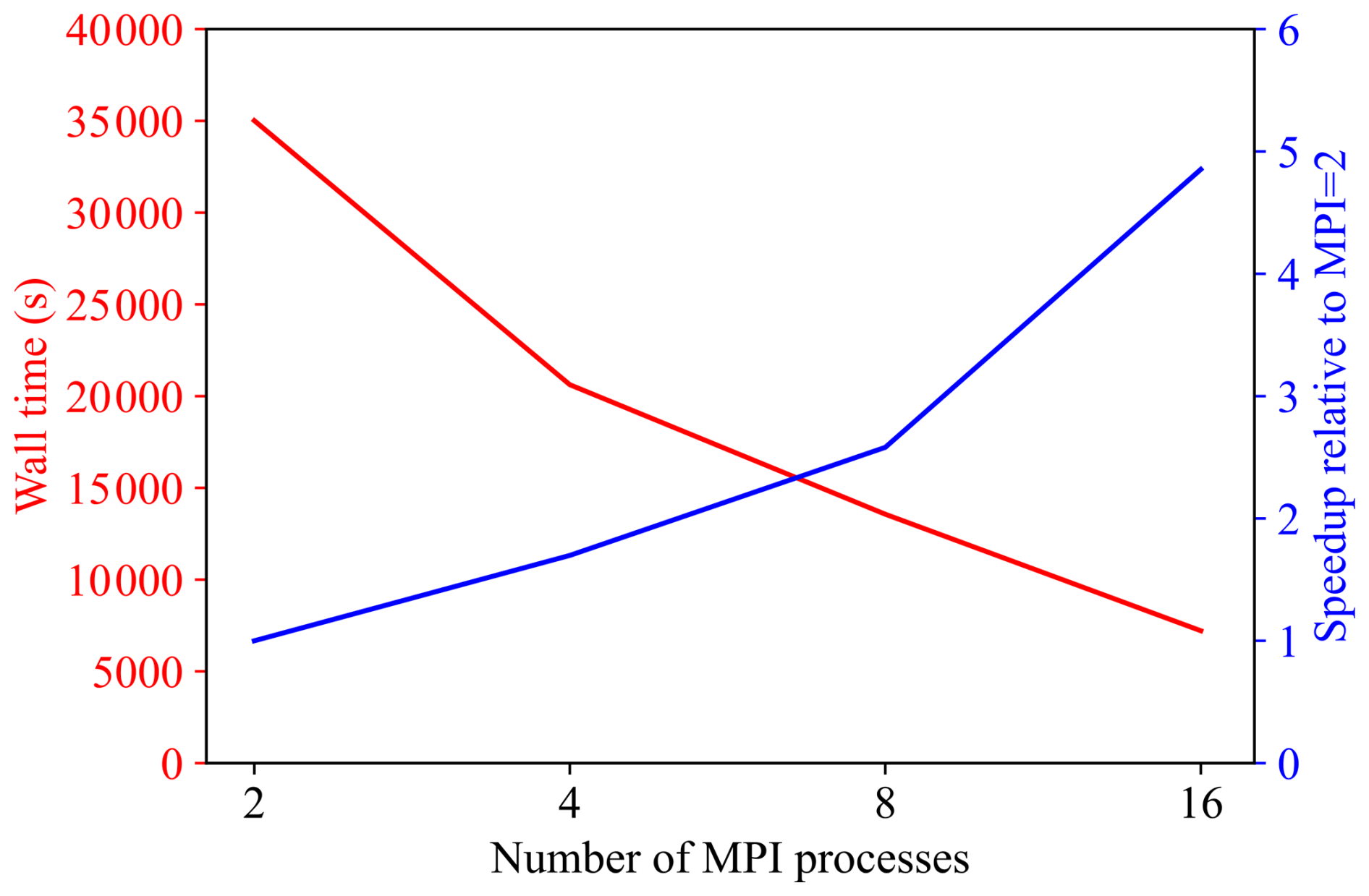
As the number of MPI processes increases from 2 to 16, the wall time decreases substantially from approximately 3.5 × 10⁴ s to below 5 × 10³ s, demonstrating a marked improvement in computational efficiency. The speedup increases monotonically over the same range and remains close to linear scaling, indicating that the developed solver is well parallelised and can effectively exploit distributed-memory computing for the problem size considered. Overall, these results confirm satisfactory strong-scaling performance up to 16 MPI processes for the 5-year simulation.

6 Conclusions

This study develops a multi-dimensional HMC modelling framework by embedding a flexible geochemical module into an existing hydro-mechanical solver, enabling a consistent treatment of multi-component aqueous species and mineral reactions in near-saturated deformable porous media. The formulation is established under small-strain assumptions and predominantly elastic behaviour, and is therefore applicable to scenarios with limited deformation.

For long-term conditions involving large settlements, plastic deformation of soft clays, or pronounced geochemical alteration, a more comprehensive framework would be required, incorporating elasto-plastic or visco-plastic constitutive behaviour together with reaction-driven porosity–permeability feedbacks. These processes are expected to intensify preferential flow pathways and enhance solute plume heterogeneity, such that neglecting them may lead to smoother transport patterns and an underestimation of plume spreading in reactive environments. Future work will focus on integrating these feedbacks and on quantitative benchmarking against laboratory and field observations to further strengthen the predictive capability of the framework.

The results show that calcite dissolution, flow-driven transport, and load-induced pore-structure evolution jointly govern both the timing and spatial distribution of solutes. Mechanical compression accelerates early-stage solute release by enhancing advective flow but later suppresses transport as porosity and flow ability decline, leading to non-monotonic concentration trends. Neglecting deformation or applying a smaller external load promotes faster mineral dissolution, whereas deformation under high load suppresses the reaction and yields a smoother dissolution front.

Saturation plays a key role in both hydro-mechanical responses and reactive-solute transport, with a more pronounced influence on chemical concentrations and plume evolution. Fully saturated soils develop the highest excess pore pressures and dissipate them most slowly, whereas lower saturation lowers the pressure peak and accelerates settlement. For solutes, decreasing saturation consistently elevates aqueous concentrations by increasing the flow velocity and concentrating dissolution-released species; this amplification is most pronounced near strong contaminant sources, which expands the high-solute and low-pH plumes laterally. Mechanical deformation counteracts this effect by reducing connected pore volume and advective transport, slightly damping concentrations, and confining plume spread.

Appendix A: List of Symbols

Sr	degree of saturation
β	compressibility of pore water (Pa−1)
vs	velocity of solid particles (m s−1)
K	hydraulic conductivity (m s−1)
Ky	K in the y direction (m s−1)
us	soil displacement (m)
uy	us in the y direction (m)
kwo	bulk modulus of pore water (MPa)
pa	apparent pressure (kPa)
μ	lamé parameter (Pa)
E	elastic modulus (Pa)
I	unit tensor
Q(t)	external loading (Pa)
ρw	density of pore fluid (kg m−3)
vf	velocity of fluid particles (m s−1)
αTH	transverse dispersion coefficient (m)
Dm	molecular diffusion coefficient (m2 s−1)
D	hydrodynamic dispersion coefficient (m2 s−1)
Ys.	mineral concentration
A0	specific surface area (m2 m${}_{\mathrm{mineral}}^{-\mathrm{3}}$)
n	soil porosity
p	excess pore water pressure (Pa)
g	gravitational acceleration (m s−2)
Kx	K in the x direction (m s−1)
Kz	K in the z direction (m s−1)
ux	us in the x direction (m)
uz	us in the z direction (m)
rh	volumetric fraction of air dissolved in pore water
p0	atmospheric pressure (kPa)
λ	lamé parameter (Pa)
G	shear modulus (Pa)
ν	Poisson's ratio
Kd	partitioning coefficient (m3 kg−1)
ρs	density of solid phase (kg m−3)
αL	longitudinal dispersion coefficient (m)
αTV	transverse dispersion coefficient (m)
$\left|\stackrel{\mathrm{‾}}{\mathbf{v}}\right|$	modulus length of the velocity (m s−1)
Y.	aqueous phase concentration (mol L−1)
J	solute flux (mol (m2 s)−1)

Appendix B: Proportion of elements diffusion coefficient

Within the coupled hydro–mechanical–chemical framework adopted in this study, the relative fractions of aqueous species ω_i, obtained from the initial geochemical speciation calculations, are prescribed as constant parameters. The effective molecular diffusion coefficient is evaluated as D_m = ${\sum }_i{\mathit{\omega }}_i{D}_{\mathrm{m}}^{\left(i\right)}$, where the species-specific diffusion coefficients $D_{\mathrm{m}}^{\left(i\right)}$ are obtained from the PHREEQC database through the -diffusion_coefficient entries. Although the present numerical architecture can, in principle, be extended to dynamically update ω_i using cell-wise speciation results from a geochemical module, such functionality is not activated in this work, because dynamic coupling would require code-level modifications and recompilation whenever the reaction network is altered, substantially reducing model reproducibility; moreover, as D_m is formulated as a weighted average of species diffusion coefficients, its variation under typical speciation changes is expected to be limited and is unlikely to affect the principal chemo-mechanical trends investigated here.

In this study, the fractions ω_i are prescribed rather than dynamically updated, as shown in Figs. B1 and B2. These figures present the compositions, fractions, and molecular diffusion coefficients of predefined species adopted in the model test cases. The values are fixed input parameters for clarity and reproducibility, but can be easily modified to represent alternative systems without changing the numerical framework. The present work primarily aims to capture the coupled deformation, solute migration, and geochemical reactions under near-saturated conditions, while dynamic updates of species fractions can be incorporated in future extensions of the same framework.

Figure B1 The proportion of elements diffusion coefficient for single mineral reaction. (a) C; (b) Ca.

Figure B2 The proportion of elements diffusion coefficient for multi-mineral reaction. (a) Al; (b) Fe.

Appendix C: Implementation of the geochemical-window controller

The geochemical-window controller (ChemWindow) schedules the activation of geochemical sub-cycling within the global hydro–mechanical–transport loop. It enables chemistry to be executed only within prescribed step-index windows, allowing kinetic reactions to be resolved with smaller time steps while maintaining an affordable global time step.

C1 Window definition and data structure

A chemistry window is defined as an inclusive index interval

$$[\mathtt{\text{start}},\mathtt{\text{end}}]\mapsto \left(\mathrm{\Delta }{t}_{\mathrm{chem}},\mathtt{\text{nSub}}\right),$$

where start and end are global OpenFOAM time indices (zero-based, inclusive), Δt_chem is the chemical sub-time-step, and nSub is the number of chemistry sub-steps executed within each global transport step. Internally, all windows are stored as a list of non-overlapping, sorted ranges.

C2 Input format and normalisation

The controller reads a plain-text input file, chemWindow.txt. Each valid entry consists of four fields, namely start, nSteps, Δt_chem, and nSub. The corresponding time window is constructed as an inclusive interval, with the ending index defined as

$$\mathtt{\text{end}}=\mathtt{\text{start}}+\mathtt{\text{nSteps}}-\mathrm{1}.$$

Basic input checks are applied, enforcing start ≥ 0, nSteps > 0, Δt_chem > 0, and nSub > 0.

An example file is

Listing C1 Example input file for chemical time stepping.

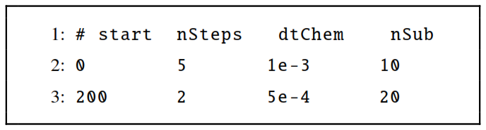
All raw windows are then normalised by: (i) stable sorting by start (and end as tie-breaker); (ii) resolving overlaps according to a user-selected conflict policy; and (iii) merging adjacent windows if they are contiguous and share identical (Δt_chem,𝚗𝚂𝚞𝚋) (within a tolerance on Δt_chem).

C3 Overlap resolution policies

If two windows overlap, the existing window is split into up to three segments (left, overlap, right). The overlap segment adopts parameters according to the selected policy:

• LastWins: parameters of the later-defined window;

• FirstWins: parameters of the earlier window;

• MinDt: window with the smaller Δt_chem;

• MaxDt: window with the larger Δt_chem.

For MinDt and MaxDt, the paired nSub from the selected record is retained; no recomputation of nSub is performed.

C4 Runtime query interface

During the global time-marching loop, the solver queries

$$\mathtt{\text{inChemWindow(currentIndex, newDt, nSub)}}.$$

A monotonic pointer to the active range is maintained, yielding amortised O(1) lookup per global step. If currentIndex satisfies start ≤ currentIndex ≤ end, the routine returns true together with (newDt, nSub); otherwise, chemistry is bypassed for this step.

A simplified driver loop is

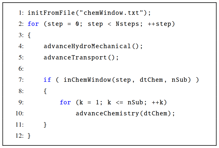
Listing C2 Simplified driver loop for coupled hydro-mechanical-transport-chemical simulation.

Appendix D: Chemical database and reaction configuration

Geochemical reactions are executed through PHREEQC using the PhreeqcRM interface. In contrast to conventional PHREEQC workflows based on standalone input scripts, the present solver introduces a dictionary-based configuration layer within OpenFOAM. Keywords such as PhreeqcDataBase and PhreeqcInputFile are parsed at runtime and directly mapped to the corresponding PhreeqcRM function calls. Consequently, all reaction systems are fully configurable at runtime, and no recompilation of the solver is required when modifying geochemical databases or reaction settings.

This design ensures that all geochemical configurations are explicitly defined within the input files, thereby enabling straightforward reproducibility of simulations while also providing high flexibility for extending reaction systems without modifying the solver source code.

D1 Database binding and runtime mapping

The thermodynamic database is specified by the keyword PhreeqcDataBase, which is passed directly to the PhreeqcRM initialisation routine. Similarly, the entry PhreeqcInputFile defines an OpenFOAM dictionary that encodes the aqueous solution composition using standard PHREEQC SOLUTION syntax. At runtime, the PhreeqcRM interface converts the dictionary entries into the corresponding PHREEQC command strings and executes them internally via PhreeqcRM, ensuring full compatibility with the official PHREEQC syntax.

D2 Reaction model configuration

Phase equilibrium and kinetic reactions are configured through the boolean flag activatePhaseEquilibrium. When enabled, mineral reactions are treated as equilibrium phases; otherwise, they are processed as kinetic reactions, reproducing the functionality of the PHREEQC blocks EQUILIBRIUM_PHASES and KINETICS. Time integration of kinetic reactions can be controlled through the options cvODE and cvODETol, which activate the CVODE integrator and prescribe its relative tolerance, respectively. The keyword setComponentH2O determines whether water is treated as an explicit geochemical component.