Nonlinear hydro-climatic controls on an arid-region lake: evidence from 40 years of remote sensing

Accurate delineation of lake surface area is fundamental for understanding eco-hydrological processes in arid regions, yet long-term lake records are often constrained by cloud contamination, seasonal ice cover, and data gaps. In this study, we develop an optimized lake-area extraction framework that integrates seasonal water-index selection, adaptive threshold segmentation, maximum connected-component analysis, and mutual-information-based image gap filling to construct a continuous monthly lake-area time series for Bahannao Lake from 1984 to 2024. This framework substantially improves the temporal continuity and robustness of long-term monitoring for small lakes in arid environments, and its regional applicability is further validated through comparative analyses with Hongjiannao Lake and Wuliangsuhai Lake. Based on the reconstructed time series, we quantitatively assess the multi-climatic controls on lake-area variability by combining correlation analysis with an XGBoost model. The results reveal pronounced seasonal differences and distinct stage-dependent evolution in lake dynamics, with the dominance alternating between precipitation-driven water input and evaporative demand across different temporal scales. Our findings highlight the nonlinear hydro-climatic responses of arid-region lakes to climate variability and provide both technical support and scientific insight for long-term lake monitoring and water-resource management in dryland regions.

1 Introduction

Over the past century, with the intensification of global climate change and the increasing human ability to modify nature, the impact of climate change on lake systems and the surrounding water environment has become more pronounced. The formation and disappearance, expansion and contraction of lakes, as well as changes in water and ecological environments, are the result of interactions among global, regional, and local tectonic activities, climate events, and human activities. Within these systems, a series of complex interactions drive the evolution of lake systems (Ma et al., 2020).

Lakes are vital natural resources that are highly sensitive to climate change (Adrian et al., 2009; Schmid et al., 2014). Globally, there are over 100 million lakes, which store 87 % of the Earth's liquid surface freshwater. Climate change is one of the most severe threats to global lake ecosystems. As observed in recent decades, lake surface conditions – such as ice cover, surface temperature, evaporation, and water levels – have responded significantly to this threat (Woolway et al., 2020; Tong et al., 2023). Approximately 53 % of the world's lakes have experienced a decline in water storage, with a reduction of about 22 billion tons per year. Climate change and human water use have primarily driven the net decrease in water volume in approximately 100 large natural lakes worldwide. Lakes in both arid and humid regions are experiencing water loss, with drying trends being more widespread than previously understood. Despite the shrinking of most lakes globally, 24 % of lakes and reservoirs have shown a significant increase in water storage. These lakes and reservoirs are mostly located in sparsely populated regions, such as the Tibetan Plateau and the northern Great Plains of North America, as well as areas with newly constructed reservoirs, including the Yangtze River, Mekong River, and Nile River basins (Pickens et al., 2020).

China has a vast territory with an extensive network of rivers and lakes. There are 2693 lakes with an area greater than 1 km², among which 2557 lakes (95 % of the total) have an area between 1 and 100 km². Additionally, there are 10 exceptionally large lakes with an area exceeding 1000 km². The total lake area in China has shown a significant increasing trend, expanding by approximately 7858.53 km² (11.41 %) over the past 30 years (Ma et al., 2010, 2011). However, the spatial and temporal imbalance of water resources has intensified, with notable differences in trends across various lake regions. The lake areas in the Tibetan Plateau and Xinjiang regions have increased significantly, contributing 111.55 % and 28.41 % of the national lake area growth, respectively. In contrast, the lake areas in the Eastern Plain, Inner Mongolia Plateau, Northeast Plain and Mountainous Region, and Yunnan-Guizhou Plateau have declined significantly, with reductions of 24.53 %, 9.30 %, 6.06 %, and 0.54 %, respectively. Among these, the Mongolian-Xinjiang Plateau experienced the largest decline in lake numbers, with a loss of 111 lakes. Some lakes in this region have shown signs of shrinkage and salinization (Yang et al., 2010). However, despite increasing attention to global lake changes, small and medium-sized closed-basin lakes in arid and semi-arid regions remain poorly characterized in long-term observations. These lakes are highly sensitive to climate variability but are often underrepresented in existing global or regional datasets, highlighting an urgent need for improved long-term monitoring.

Scientists have discovered that the abrupt change timing of river and lake systems varies significantly across different latitudes and altitudes (Råman Vinnå et al., 2021; Zhou et al., 2021). Mountain and polar lakes tend to experience abrupt changes earlier than temperate and tropical river-lake systems (Jeppesen et al., 2014). Additionally, under varying levels of human impact, the timing of abrupt changes in lakes also differs. Lakes in regions with low human impact generally experience abrupt changes earlier than those in areas with strong human influence (Preston et al., 2016). Analysis of the driving factors of lake abrupt changes indicates that the causes vary. Before the 1950s, climate change was the primary factor controlling abrupt changes in lake ecosystems. However, after the 1950s, both climate change and human disturbances became dominant factors. In temperate and tropical regions with strong human influence, lake changes are mainly driven by nutrient enrichment and pollution. In contrast, lakes located in high-altitude and high-latitude regions, which are less affected by human activities, are more vulnerable to climate change. Furthermore, the interaction of multiple drivers increases the likelihood of abrupt changes in lakes, with climate change being the most frequently interacting factor leading to transformations in river-lake ecosystems (Vincent, 2009). Li et al. (2025) pointed out that seasonality is the dominant driver of lake-surface-extent variations globally.

For example, Plug et al. (2008) investigated lake area changes in the Tuktoyaktuk Peninsula in northwest Canada. They found that from 1978 to 1992, the total lake area increased, while from 1992 to 2001, the total lake area decreased. Their study identified precipitation as the main factor driving these changes. Similarly, Carroll et al. (2011) studied the lake area changes in high-latitude northern Canada and discovered that lake areas showed a significant decline, exhibiting regional clustering characteristics, with climate factors driving these changes. Laba et al. (2017) explored the expansion of Tangra Yum Co from 1977 to 2014. Their results indicated that, under the background of climate warming, the combined effects of glacier melt, precipitation increase, and evaporation changes contributed to the lake's expansion. Likewise, Li et al. (2017) examined the changes in the water surface area and water storage of Nam Co from 1976 to 2015. Their findings showed that the water surface area and water storage of Nam Co continued to increase, with the fastest growth in water storage occurring between 1997 and 2009. The study concluded that the primary factor driving the increase in Nam Co's water volume was glacier melt, followed by increased precipitation and reduced evaporation.

However, the precise measurement of lake area remains a major constraint for analyzing lake changes. With advancements in science and technology, remote sensing has provided a unique and effective method for monitoring the spatiotemporal variations in surface water areas on broad geographic scales (Liu et al., 2020).

Currently, water extraction methods using optical sensors have been widely applied (McFeeters 1996; Yao et al., 2015; Donchyts et al., 2016). However, existing water body area products often fail to meet ideal spatial or temporal resolution requirements (Cooley et al., 2017; Huang et al., 2018). For example, the 2016 Global Climate Observing System (GCOS) Implementation Plan recommended a resolution of 20 m and a daily monitoring frequency (Secretariat, 2009). High-temporal-resolution sensors, such as the Moderate Resolution Imaging Spectroradiometer (MODIS) onboard Terra and Aqua satellites, have been used to assess water body areas at time scales ranging from daily to 16 d intervals (Bergé-Nguyen and Crétaux, 2015; Wang et al., 2018a). However, many small water bodies (e.g., 10–50 km² or smaller) and irregularly shaped larger water bodies may not be accurately distinguished using coarse-resolution MODIS images (250–500 m in the visible and near-infrared bands) (Tao et al., 2015). Compared with MODIS, Landsat images (e.g., Landsat 5 Thematic Mapper (TM), Landsat 7 Enhanced Thematic Mapper Plus (ETM+), and Landsat 8 Operational Land Imager (OLI)) offer higher spatial resolution (30 m) and a temporal resolution of 16 d (or better when combining multiple Landsat sensors). However, due to cloud contamination (Rossow and Schiffer, 1999), the actual temporal frequency of water body mapping based on Landsat is often much lower than the nominal resolution and may extend to a year for lakes with persistent ice cover (Yao et al., 2018). The recently launched Sentinel-2A and 2B satellites, equipped with Multispectral Instruments (MSI), provide a resolution of 10 m in the visible and near-infrared bands, with a revisit period of 5–10 d. However, their observations currently cover only the past few years (since 2015) and are not yet suitable for long-term decadal monitoring.

Beyond the trade-offs between spatial and temporal resolution, several other factors challenge high-resolution monitoring of long-term global surface water area changes (Klein et al., 2017). These include the inherent spectral heterogeneity of water, atmospheric influences (clouds and aerosols), topographic shadows, aquatic vegetation, and spectral contamination from ice/snow cover. In such complex conditions, integrating multiple techniques is often necessary to achieve robust water body extraction.

Recently, Pekel et al. (2014) utilized a large training dataset, combined with expert systems and visual analysis, to identify the presence or absence of water on a monthly basis for each pixel in archival Landsat images from 1984 to 2015. This product was named the Joint Research Centre (JRC) Global Surface Water dataset (hereinafter referred to as GSW). Despite its significant achievements, GSW is based on cloud-free pixels, meaning that the mapped extent of specific water bodies is only complete when monthly composite images have minimal cloud cover. A follow-up study by Busker et al. (2019) used a subset of the GSW dataset, selecting images with cloud cover below 5 %, to extract the monthly area of 137 lakes/reservoirs. For nearly half of these lakes/reservoirs, the correlation between area and radar altimetry-measured water levels exceeded 0.8. However, the temporal frequency of the resulting area time series was still constrained by the availability of cloud-free images, and due to the current availability of GSW, the time series was interrupted after October 2015.One potential method to increase the temporal frequency of lake mapping based on Landsat data is to estimate water surface area from contaminated images (e.g., those affected by clouds or observation gaps). Although these images are of relatively lower quality, the exposed portions of lakes within them may provide useful information for inferring the complete extent. For instance, Zhao and Gao (2018) 41 applied the monthly water mapping data from the GSW dataset to generate area time series for 6,817 reservoirs worldwide from 1984 to 2015. Their method involved recovering complete reservoir extents from cloud-contaminated images by segmenting pixels based on the water occurrence probability provided in the GSW dataset. Compared to the results of Busker et al. (2019), their generated area time series increased the number of observations by approximately 80 %. However, the reliance on the existing GSW dataset restricted their reservoir area records to the 1984–2015 period, and the validation of their recovery method was limited to only nine reservoirs with significant water level variations. These studies demonstrate the feasibility of large-scale lake monitoring, but also highlight persistent limitations related to temporal continuity, cloud dependence, and the applicability of existing products to small lakes. As a result, many existing lake-area studies rely on annual or seasonal snapshots derived from a limited number of cloud-free images, which may obscure important intra-annual variability, abrupt changes, and short-term climate responses, particularly for small lakes with strong seasonal dynamics.

To address this limitation, we construct a continuous 40-year monthly lake-area time series for Bahannao Lake by integrating multi-source Landsat imagery and applying a tailored image-processing workflow. This higher-temporal-resolution dataset enables a more detailed assessment of seasonal and interannual lake dynamics.

Bahannao Lake is a small closed-basin lake located in a semi-arid desert region of northern China. Owing to its remote location and the long-term absence of systematic in situ observations, continuous records of lake area are lacking. Nevertheless, as a water body embedded in a fragile desert ecosystem, variations in lake area are highly sensitive to hydro-climatic changes and play an important role in regional eco-hydrological stability.

In recent decades, intensified warming and drying have caused pronounced lake shrinkage, characterized by strong interannual variability and multiple abrupt changes. However, compared with larger or well-monitored lakes, the dynamic behavior and driving mechanisms of Bahannao Lake remain poorly understood due to the lack of long-term, high-temporal-resolution observations. As a typical but underrepresented small lake in arid regions, Bahannao Lake provides an ideal case for testing robust remote-sensing monitoring methods and investigating hydro-climatic controls on dryland lake dynamics.

Despite substantial progress in global lake monitoring, significant gaps remain for lakes in arid and semi-arid regions. Long-term and continuous lake area records are often interrupted by cloud contamination, seasonal ice cover, and striping artifacts, while the role of hydro-climatic drivers – particularly their nonlinear interactions – remains insufficiently understood.

To address these challenges, this study develops an optimized lake area extraction framework that integrates seasonal index selection, adaptive thresholding, connectivity analysis, and mutual information–based gap filling to construct a continuous monthly lake-area record for Bahannao Lake from 1984 to 2024. By coupling this reconstructed time series with multi-factor analysis using the XGBoost model, we quantify the relative importance and nonlinear effects of key hydro-climatic drivers on lake dynamics. This framework not only improves the reliability of long-term lake monitoring under complex conditions, but also provides new insights into seasonal and interannual climate controls on small lakes in arid and semi-arid regions.

2 Data and Methods

2.1 Study area and data

Closed-basin lakes of various sizes are widely distributed across the Ordos Plateau, formed since the late Quaternary through combined aeolian and fluvial erosion processes. Bahannao Lake is the terminal basin of a chain of seven bead-like erosional lake depressions that developed along an ancient river valley. Bahannao Lake (109°16^′ E, 39°19^′ N) is located in the central Ordos Plateau at an elevation of 1278 m, with a lake-basin area of 26.50 km². The basin is underlain by a continuous and intact Lower Cretaceous sandstone formation, which provides a closed geomorphic setting primarily recharged by atmospheric precipitation. The sandstone contains abundant sodium- and calcium-rich carbonates, serving as the major source of dissolved salts in Bahannao Lake. Administratively, the study area belongs to Wushen Banner of the Ordos region in Inner Mongolia (Fig. 1).

The zonal vegetation is dominated by arid to semi-arid desert steppe. The region is controlled for most of the year by the northwesterly monsoon, resulting in a cold and dry climate, while the southeasterly monsoon occasionally influences the area and plays a decisive role in seasonal precipitation. The mean annual temperature ranges from 6 to 9 °C, and the mean annual precipitation is only 200–300 mm, concentrated mainly from June to September with short-duration high-intensity rainfall events. In contrast, the annual potential evaporation reaches 2500–3000 mm, approximately ten times the precipitation amount, and the regional aridity index ranges from 3.5 to 4.0.

Because of the extremely fragile water balance and rapid hydrological response to climatic anomalies, Bahannao Lake and other nearby lakes are widely recognized as important natural indicators of climate variability, drought intensification, and land–atmosphere interactions in the arid and semi-arid regions of northern China.

This study utilizes remote sensing imagery from the Landsat 5 TM, Landsat 7 TM, and Landsat 8 OLI sensors, specifically using atmospherically corrected reflectance data (Tier 1 TOA Reflectance). Tier 1 data is selected due to its highest quality, making it suitable for time-series analysis and studies on global surface water extent and dynamics. The Landsat 5 TM imagery covers the period from 1984 to 2011, while Landsat 8 imagery spans from 2013 to 2023. Since imagery for 2012 is missing in both datasets, Landsat 7 TM is used as a supplement. However, Landsat 7 TM imagery exhibits significant striping artifacts, which were avoided as much as possible during data selection.

For hydro-climatic elements, this study employs the fifth-generation atmospheric reanalysis dataset from ECMWF (European Centre for Medium-Range Weather Forecasts), covering global climate data from January 1950 to the present. The dataset has a temporal resolution of daily and a spatial resolution of 0.1° × 0.1°. The hydro-climatic variables used in this study include precipitation (P, mm), air temperature at 2 m (T, °C), 2 m dew point temperature (T_d, °C), relative humidity (RH, %), potential evapotranspiration (PET, mm), net shortwave radiation at the surface (msnswrf, W m⁻²), net longwave radiation at the surface (msnlwrf, W m⁻²), surface latent heat flux (mslhf, W m⁻²), and surface sensible heat flux (msshf, W m⁻²). These variables jointly characterize atmospheric moisture conditions, energy balance, and evaporative demand in the study region.

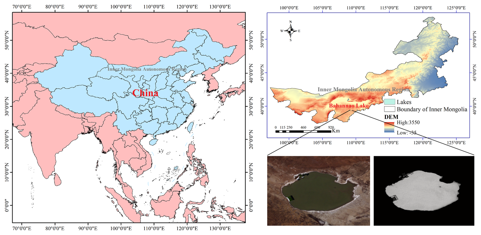
Figure 1 Overview map of the study area. Source: U.S. Geological Survey (USGS). Data are in the public domain.

2.2 Methods

2.2.1 Optimized lake area extraction method

Although water-index-based lake extraction from Landsat imagery is well established, long-term monthly monitoring of small lakes in arid regions poses specific challenges, including frequent cloud contamination, striping artifacts in ETM+ data, and strong intra-annual variability. To address these issues, we developed an optimized processing workflow tailored to long-term monthly lake monitoring.

This study employs 30 m full-atmosphere imagery from the Landsat 5 Thematic Mapper (TM), Landsat 7 Enhanced Thematic Mapper Plus (ETM+), and Landsat 8 Operational Land Imager (OLI) satellites to derive monthly lake area estimates for the study region from January 1984 to December 2024.

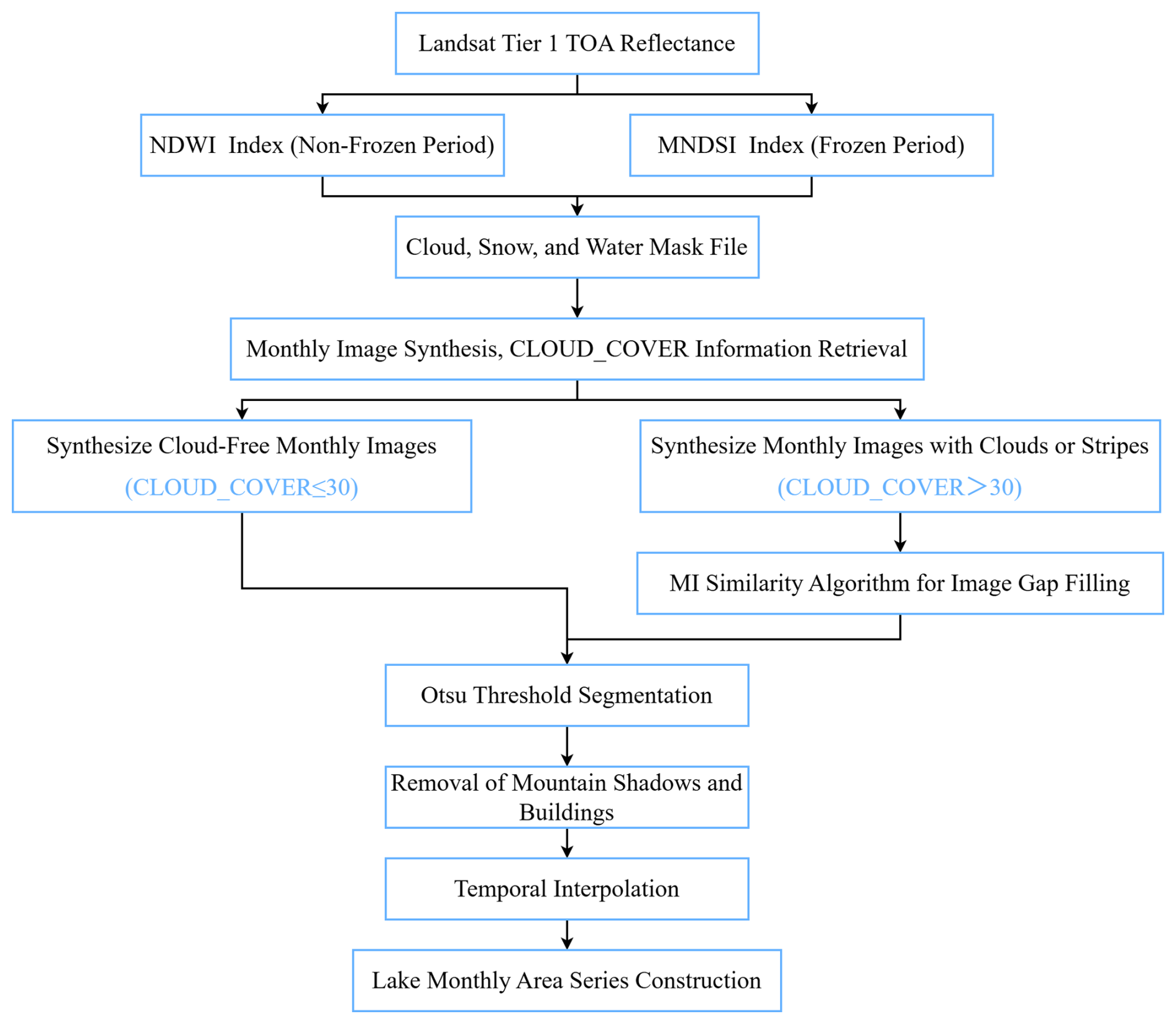
Different lake remote sensing indices were selected for non-freezing and freezing periods, respectively. For non-freezing periods, remote sensing indices were processed to remove cloud and snow interference. Images were filtered based on cloud cover percentage (C), and monthly composite images were generated. The Otsu thresholding method was then applied to automatically determine segmentation thresholds. To distinguish between lakes and mountainous areas, a digital elevation model (DEM) was used, setting the slope (θ) and aspect (ϕ) thresholds to 0.

Considering that most lakes exhibit connectivity, this study adopts the maximum connected component analysis algorithm from the OpenCV computer vision library to delineate lake boundaries. Images were categorized based on cloud cover information (“CLOUD_COVER”): those with cloud cover ≤30 % were classified as cloud-free images, while the remaining images were considered cloudy. For cloudy images, the MI (Mutual Information) algorithm was used to match them with the most similar cloud-free images. The most similar image was then merged with the original cloudy image to generate a filled version.

For images with striping artifacts, the same filling method was applied as for cloudy images. Clear lake boundaries from historical cloud-free images were used, and the MI algorithm was employed to find the most similar historical cloud-free images for filling missing water pixels in striped areas, ultimately obtaining the final lake water extent. The specific process is shown in Fig. 2.

Figure 2 Flowchart of lake area extraction process.

2.2.2 Aridity index (AI)

The aridity index (AI) was used to quantify regional drought conditions. AI is defined as the ratio of precipitation (P) to potential evapotranspiration (PET), expressed as:

$$\begin{array}{}\text{(1)}& \text{AI}={\displaystyle \frac{P}{\text{PET}}}\end{array}$$

where P represents precipitation and PET denotes potential evapotranspiration. AI reflects the balance between atmospheric water supply and evaporative demand.

In this study, PET was calculated using the FAO Penman–Monteith method, which is widely recognized as a physically based and robust approach for estimating atmospheric evaporative demand. PET was computed as:

$$\begin{array}{}\text{(2)}& \text{PET}={\displaystyle \frac{\mathrm{0.408}\mathrm{\Delta }(R_{\mathrm{n}}-G)+\mathit{\gamma }\frac{\mathrm{900}}{T+\mathrm{273}}{u}_{\mathrm{2}}(e_{\mathrm{s}}-e_{\mathrm{a}})}{\mathrm{\Delta }+\mathit{\gamma }(\mathrm{1}+\mathrm{0.34}{u}_{\mathrm{2}})}}\end{array}$$

Where R_n is the net radiation at the surface (MJ m⁻² d⁻¹), G is the soil heat flux (MJ m⁻² d⁻¹), T is the mean air temperature at 2 m height (°C), u₂ is the wind speed at 2 m height (m s⁻¹), e_s is the saturation vapor pressure (kPa), e_a is the actual vapor pressure (kPa), Δ is the slope of the saturation vapor pressure–temperature curve (kPa °C⁻¹), and γ is the psychrometric constant (kPa °C⁻¹).

All meteorological variables required for PET estimation were obtained from the ERA5 reanalysis dataset and spatially averaged over the study area to ensure consistency with basin-scale analysis.

Based on AI values, climatic conditions were classified following the United Nations Environment Programme (UNEP) scheme: AI <0.05 indicates hyper-arid conditions, $\mathrm{0.05}\le \text{AI}<\mathrm{0.20}$ represents arid conditions, $\mathrm{0.20}\le \text{AI}<\mathrm{0.50}$ corresponds to semi-arid conditions, $\mathrm{0.50}\le \text{AI}<\mathrm{0.65}$ indicates dry sub-humid conditions, and AI ≥0.65 represents humid conditions. This classification allows a quantitative interpretation of regional aridity and facilitates comparison with previous studies in arid and semi-arid regions.

2.2.3 XGBoost Model

In this study, the XGBoost model is employed primarily as an interpretative tool. The objective is to quantify the relative importance of different hydro-climatic factors and to explore potential nonlinear relationships between lake-area variability and climatic drivers. Given the limited sample size, strong interannual variability, and high nonlinearity characteristic of arid-region lake systems, model performance metrics (e.g., R²) are used as auxiliary indicators, while greater emphasis is placed on feature-importance rankings for mechanism interpretation.

Compared with linear correlation analysis, the XGBoost results highlight the importance of nonlinear and season-dependent controls, particularly during transitional seasons when linear correlations are weak. This demonstrates the added value of XGBoost in revealing climatic influences that cannot be fully captured by linear statistical methods alone.

The objective function of the XGBoost model is:

$$\begin{array}{}\text{(3)}& L\left(\mathit{\theta }\right)=\sum _{i=\mathrm{1}}^{n}l(y_i,f(x_i\left)\right)+\sum _{i=\mathrm{1}}^n\mathrm{\Omega }\left(f_k\right)\end{array}$$

Where L(θ) represents the objective function, which measures the model's performance in prediction and consists of two parts: l(y_i,f(x_i)) is the loss function, indicating the difference between the true value y_i and the predicted value f(x_i), while Ω(f_k) is the regularization term used to control the model complexity.

The input factors $x_i=\left\{x_{\mathrm{1}},x_{\mathrm{2}},\mathrm{\dots },x_n\right\}$ include precipitation (P), air temperature (T), relative humidity (RH), and potential evapotranspiration (PET), which represent the primary components of the lake water balance in arid and semi-arid regions. These variables directly or indirectly regulate lake-area changes through their influence on water input and evaporative loss. Energy-related variables (e.g., radiation and heat fluxes) are included as background indicators of atmospheric conditions and are not interpreted as direct driving forces of lake-area change.

$$\begin{array}{}\text{(4)}& \text{FI}\left(x_j\right)={\displaystyle \frac{\mathrm{1}}{T}}\sum _{t=\mathrm{1}}^{T}I(t,x_j)\end{array}$$

Here, FI(x_j) represents the feature importance of factor x_j, while I(t,x_j) denotes the contribution of factor x_j when used as a splitting point in tree t, with T being the total number of trees. The generated feature importance ranking chart illustrates the contribution of various input factors (such as temperature, precipitation, and humidity) to lake area changes. This ranking chart provides an intuitive way to identify the most influential factors.

To improve model performance, hyperparameters can be optimized using Grid Search or Random Search. Common hyperparameters include Learning rate, Max depth of trees and Number of trees. Adjusting these parameters affects the model's fitting ability and generalization performance.

Data Splitting. Divide the dataset into a training set and a test set (e.g., 80 % for training, 20 % for testing).

Train the XGBoost model on the training set. XGBoost uses the Gradient Boosting Algorithm, which iteratively improves the model by building multiple weak learners to reduce prediction errors. Each iteration refines the model by fitting the residuals (i.e., prediction errors).

Model Validation. Evaluate model performance using metrics such as Mean Squared Error (MSE) and Coefficient of Determination (R²) to assess accuracy and stability.

The formula for Mean Squared Error (MSE) is:

$$\begin{array}{}\text{(5)}& \text{MSE}={\displaystyle \frac{\mathrm{1}}{n}}\sum _{i=\mathrm{1}}^n(y_i-f(x_i){)}^{\mathrm{2}}\end{array}$$

The formula for the coefficient of determination R² is:

$$\begin{array}{}\text{(6)}& R^{\mathrm{2}}=\mathrm{1}-{\displaystyle \frac{\sum _{i=\mathrm{1}}^n(y_i-f(x_i){)}^{\mathrm{2}}}{\sum _{i=\mathrm{1}}^n(y_i-\overline{y}{)}^{\mathrm{2}}}}\end{array}$$

Where $\overline{y}$ represents the mean of the samples.

The lake area model is based on model training, the predicted lake area $\widehat{y}$ can be expressed as a nonlinear combination of input factors x_i:

$$\begin{array}{}\text{(7)}& \widehat{y}=f\left(x_i\right)=\sum _{k=\mathrm{1}}^K{\mathit{\omega }}_k{h}_k\left(x_i\right)\end{array}$$

Where: ω_k is the weight of the k tree, and h_k(x_i) is the prediction function of the tree, represented as a set of decision rules.

The feature importance derived from the XGBoost model reflects the relative contribution of each climatic variable in reducing prediction error across all decision trees. It should be noted that this importance ranking does not imply direct causality, but rather indicates the sensitivity of lake-area variability to different climatic factors under nonlinear interactions. Therefore, feature importance is interpreted in conjunction with linear correlation analysis to provide a more robust understanding of hydro-climatic controls.

3 Lake area time series construction

3.1 Remote sensing interpretation and monthly lake image synthesis

3.1.1 Selection of water indices and image preprocessing

The study area is located in a high-altitude region, where lake surfaces freeze between November and March. Since the NDWI index is less effective for frozen lakes, different indices are used for different seasons. During the non-freezing period (May–November), the NDWI index is applied for conventional water body extraction. During the freezing period (December–April), the Modified Normalized Difference Snow Index (MNDSI) is used to evaluate water surface area.

The NDWI index utilizes the strong absorption of water bodies in the near-infrared band and their high reflectance in the green band to enhance the distinction between water and other land cover types. However, this index may misidentify bright white buildings, clouds, snow, and mountain shadows as water bodies. Therefore, additional data quality bands and methods are integrated to remove these interferences and improve the accuracy of water body extraction.

$$\begin{array}{}\text{(8)}& \text{NDWI}={\displaystyle \frac{(\text{Green}-\text{NIR})}{(\text{Green}+\text{NIR})}}\end{array}$$

Where: Green band typically refers to the green portion of the visible spectrum, generally ranging from 500–570 nm. NIR band refers to the near-infrared spectrum, generally ranging from 800–900 nm.

The Modified Normalized Difference Snow Index (MNDSI) is an index calculated using the reflectance of the near-infrared (NIR) and short-wave infrared (SWIR) bands. It is an effective method for distinguishing ice surfaces from water bodies. This index is particularly suitable for regions with frozen water surfaces, such as lakes and rivers, where seasonal changes are significant. Ice surfaces and water bodies have different reflectance characteristics in various bands. Ice has higher reflectance in the SWIR band, while water has lower reflectance. By calculating the difference between the NIR and SWIR bands, MNDSI can effectively distinguish between ice surfaces and water bodies, thus improving the accuracy of ice extraction. By combining these two bands, MNDSI highlights the differences between water bodies and ice surfaces, making it easier to differentiate between them. Similar to NDWI, MNDSI enhances the contrast between ice and water by utilizing reflectance values from different bands.

MNDSI (Modified Normalized Difference Snow Index) is calculated by combining the reflectance of the near-infrared (NIR) and short-wave infrared (SWIR) bands. The typical formula for MNDSI is as follows:

$$\begin{array}{}\text{(9)}& \text{MNDSI}={\displaystyle \frac{\text{NIR}-\text{SWIR}}{\text{NIR}+\text{SWIR}}}\end{array}$$

Where NIR is the reflectance in the near-infrared band (typically 800–900 nm), SWIR is the reflectance in the short-wave infrared band (typically 1500–1700 nm).

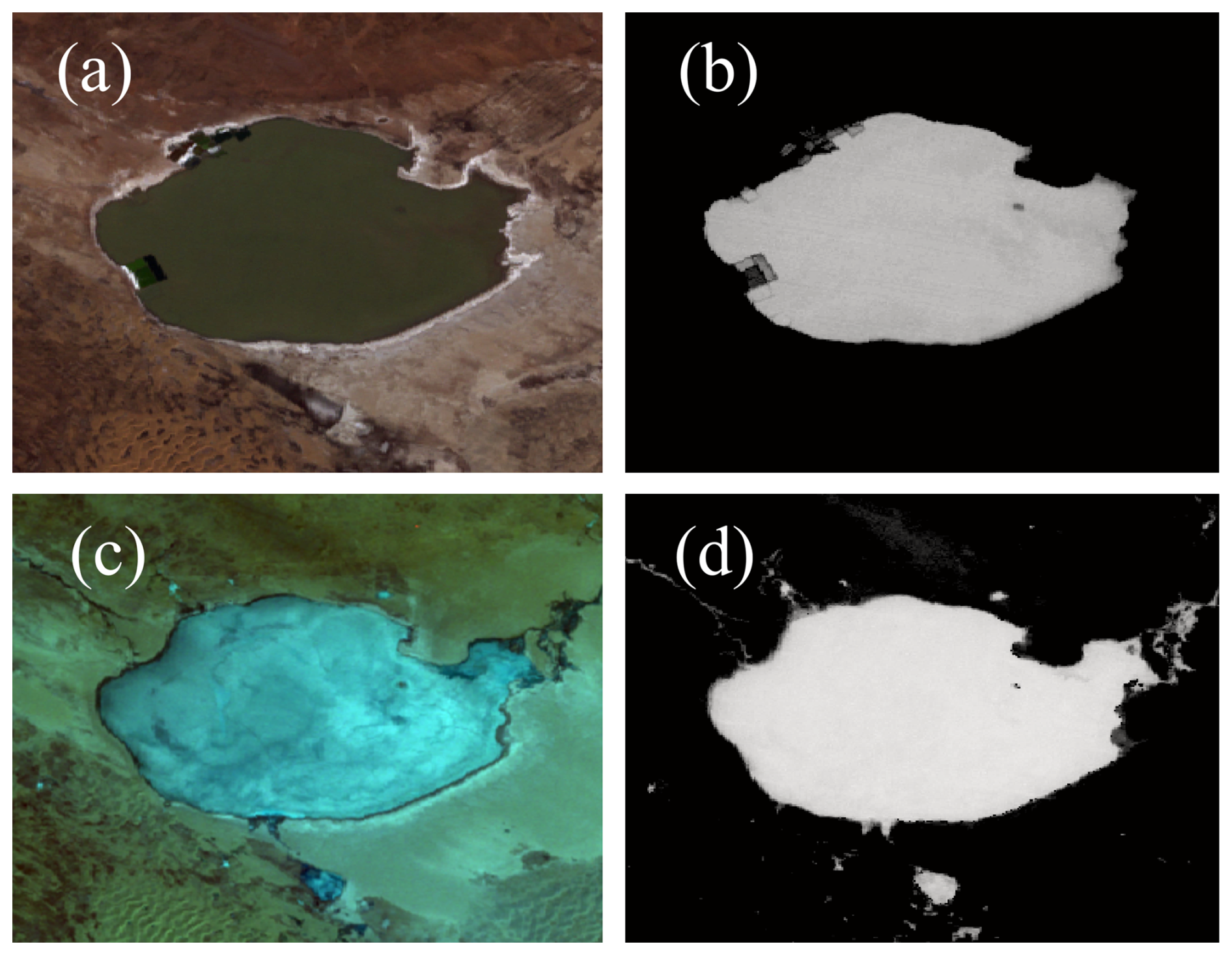
Figure 3 Lake extraction from Landsat imagery during non-freezing and freezing periods. (a) Original Landsat image during the non-freezing period; (b) Lake area identified using NDWI; (c) Original Landsat image during the freezing period; (d) Lake area identified using MNDSI. Source: Landsat imagery courtesy of the U.S. Geological Survey (USGS), processed and interpreted by the authors.

The cloud and snow interference removal is only applied to the NDWI of the non-freezing period from May to November. The Landsat series satellites provide their own pixel-scale data quality band (QA_PIXEL), which can be used to eliminate noise pixels in the image.

The QA_PIXEL band in the Landsat dataset provides information on various quality types, where different bits (Bit) correspond to different types of quality information. For example, Bit 3 corresponds to clouds, Bit 5 corresponds to snow, and Bit 7 corresponds to water bodies. Within the same bit, values of 0 and 1 represent different data qualities. For example, a 0 in Bit 7 indicates that the pixel has poor water body information, being land or covered by clouds, while a 1 indicates that the pixel represents water.

Using this pixel quality information, we selected Bit 3 (cloud), Bit 5 (snow), and Bit 7 (water body). By performing bitwise AND and OR operations, we generated a water body mask file with good data quality after cloud and snow removal. This mask file is then overlaid with the actual image to remove pixels affected by cloud or snow interference. The effect of cloud and snow removal is shown in Fig. 4.

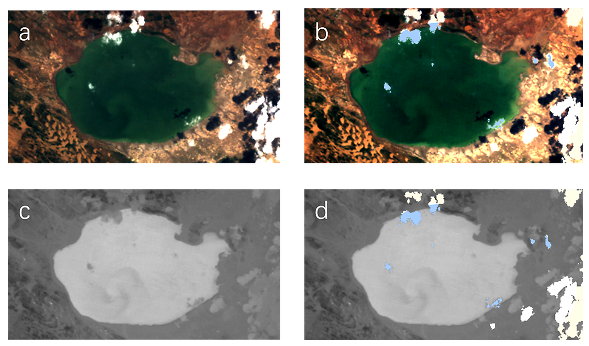
Figure 4 Illustration of cloud and snow removal and its effect on NDWI-based water extraction. (a) True-color Landsat image before cloud and snow removal. (b) True-color image after cloud and snow masking, where contaminated pixels are excluded. (c) NDWI image derived from the original true-color image, shown in grayscale, with brighter values indicating higher likelihood of water presence. (d) NDWI image after cloud and snow removal; blue areas indicate pixels affected by cloud or snow that were excluded from water-body extraction. Source: Landsat imagery courtesy of the U.S. Geological Survey (USGS), processed and interpreted by the authors.

The NDWI, MNDSI index calculation, and cloud/snow interference removal are performed directly on the GEE platform, followed by monthly composite image downloads. Based on the cloud cover information (“CLOUD_COVER”), which represents the cloud amount (range from 0 to 100, with larger values indicating more cloud coverage), the data is classified into three levels: 0–30, 30–60, and 60–100. If data is available in Level 1, Level 2 is not executed, and if Level 2 contains data, Level 3 is processed. All images from each year and month within the cloud cover level are selected, and the median pixel value is calculated to generate the composite monthly NDWI (for 5–11 months) and MNDSI (for December to the following April) grayscale images.

Data is filtered based on the cloud cover proportion C, where $C\in [\mathrm{0},\mathrm{100}]$.

Composite image =Med(S(C)), where C=CLOUD_COVER

$$\begin{array}{}\text{(10)}& S\left(C\right)=\left\{\begin{array}{lll}I\left(C\right)& \text{ if}& \mathrm{0}\le C\le \mathrm{30}\\ I\left(C\right)& \text{ else if}& \mathrm{30}<C<\mathrm{60}\\ I\left(C\right)& \text{ else}& \mathrm{60}<C\le \mathrm{100}\end{array}\right.\end{array}$$

Where I(C) is a set of image data filtered by cloud cover.

3.1.2 Threshold-based water segmentation and noise removal

Lake water pixels were first identified using threshold-based segmentation. To reduce false positives caused by mountain shadows and built-up areas, topographic and ancillary data were applied to remove non-water pixels.

1. Threshold segmentation. This step applies the Otsu threshold algorithm to the downloaded NDWI and MNDSI monthly composite grayscale images, automatically generating a segmentation threshold. Pixels below the threshold are classified as water, and those above the threshold are classified as other areas.

   The core of the Otsu thresholding method is to divide the image into two classes (foreground and background) by maximizing the between-class variance, thereby achieving the optimal threshold segmentation. Specifically, it involves iterating through all possible thresholds, and the optimal threshold is determined when the between-class variance is maximized while the variance within both the foreground and background is minimized. Compared to other methods, this algorithm maximizes the inclusion of the target feature while excluding other interfering factors.

   The Otsu thresholding method is used to automatically generate the segmentation threshold, dividing the image into water and other regions:

   $$\begin{array}{}\text{(11)}& T=\arg max\underset{\mathit{\tau }}{max}\left({\mathit{\sigma }}_B^{\mathrm{2}}\right(\mathit{\tau }\left)\right)\end{array}$$

   Where, ${\mathit{\sigma }}_B^{\mathrm{2}}\left(\mathit{\tau }\right)$ is the between-class variance, defined as:

   $$\begin{array}{}\text{(12)}& {\mathit{\sigma }}_B^{\mathrm{2}}\left(\mathit{\tau }\right)={\mathit{\omega }}_{\mathrm{1}}\left(\mathit{\tau }\right){\mathit{\omega }}_{\mathrm{2}}\left(\mathit{\tau }\right)\left(\mathit{\mu }{}_{\mathrm{1}}\right(\mathit{\tau })-{\mathit{\mu }}_{\mathrm{2}}(\mathit{\tau }){)}^{\mathrm{2}}\end{array}$$

   Where ω₁(τ) and ω₂(τ) are the weights of the foreground and background at the threshold τ, and μ₁(τ) and μ₂(τ) are the mean gray values of the foreground and background, respectively.

   The portion smaller than the threshold T is classified as water, symbolized as water pixels, while the portion greater than the threshold is classified as other categories.

2. Mountain shadow and buildings removal. Since the lake surface typically exhibits a flat state without significant slope and aspect features, digital elevation models (DEM) can be used to distinguish lakes from mountainous regions by utilizing slope and aspect information. By setting threshold values of 0 for slope and aspect, the distinction between lakes and mountainous areas can be made. However, the current frequency of elevation data updates does not align with real-time imagery, leading to an inability to accurately reflect seasonal changes in lake water levels within the elevation data. This limitation affects the precision of water body area extraction using the data. Given that most lakes are interconnected, this study employs the maximum connected component analysis algorithm from the Open-CV vision field to define the boundaries of lakes and extract their areas.

   By setting the thresholds for slope θ and aspect φ to 0 in the digital elevation model (DEM), lakes are distinguished from mountainous areas:

   $$\begin{array}{}\text{(13)}& \mathit{\theta }(x,y)=\mathrm{0},\mathit{\varphi }(x,y)=\mathrm{0}\end{array}$$

   Where θ(x,y) and ϕ(x,y) represent the slope and aspect values at a given point (x,y), respectively. By setting $\mathit{\theta }(x,y)=\mathrm{0}$ and $\mathit{\varphi }(x,y)=\mathrm{0}$ as threshold conditions for the lake area, the lake region is defined as the area where both the slope and aspect are equal to 0.

   $$\begin{array}{}\text{(14)}& L=\underset{i}{max}\left(\sum _{x,y\in C_i}I(x,y)\right)\end{array}$$

   Where L represents the total number of pixels in the largest lake area, C_i represents the ith connected component in the image, the function ∑ denotes the summation of pixel points, and $\underset{i}{max}$ indicates the selection of the largest connected component as the lake area.

   The construction of the building index currently mainly relies on the fact that the surface temperature of buildings is usually higher than that of surrounding land cover, and the mid-infrared band can effectively reflect surface temperature differences. However, in previous land cover classification studies, the extraction results using this algorithm were not ideal. Considering that most buildings in the study area are not distributed along lakes, the maximum connected component algorithm can effectively exclude parts where buildings are misidentified as water bodies.

   Based on the NDWI (Normalized Difference Water Index), a threshold T is used to binarize the image, separating water bodies from non-water bodies.

   $$\begin{array}{}\text{(15)}& I(x,y)=\left\{\begin{array}{ll}\mathrm{1},& \text{if NDVI}(x,y)>T\\ \mathrm{0},& \text{if NDVI}(x,y)\le T\end{array}\right.\end{array}$$

   Connected Component Calculation: In the binarized image, the Connected Components Labeling (CCL) algorithm is used to identify all connected regions. A connected component is determined by scanning the neighboring pixels in the image (up, down, left, right, or diagonally). The formula is expressed as:

   $$\begin{array}{}\text{(16)}& C_i=\sum _{(x,y)\in R}I(x,y)\end{array}$$

   Where R represents the connected regions in the image, and C_idenotes the connected components.

   To eliminate interference from buildings, a threshold condition τ is set, retaining only connected components with an area greater than τ. Since buildings typically have smaller areas, while lakes exhibit larger connected components, the lake regions can be filtered using the following condition:

   $$\begin{array}{}\text{(17)}& C_i>\mathit{\tau }\end{array}$$

   The lake boundary is extracted using a boundary detection algorithm (e.g., the Canny edge detection algorithm) applied to the selected largest connected region.

   $$\begin{array}{}\text{(18)}& B=\text{Canny}\left(C_i\right)\end{array}$$

   As shown in the Fig. 5, the white areas in the original image include both lakes and buildings. When using threshold segmentation to extract water bodies, buildings may also be mistakenly identified as water. By applying the maximum connected component method, buildings can be effectively separated.

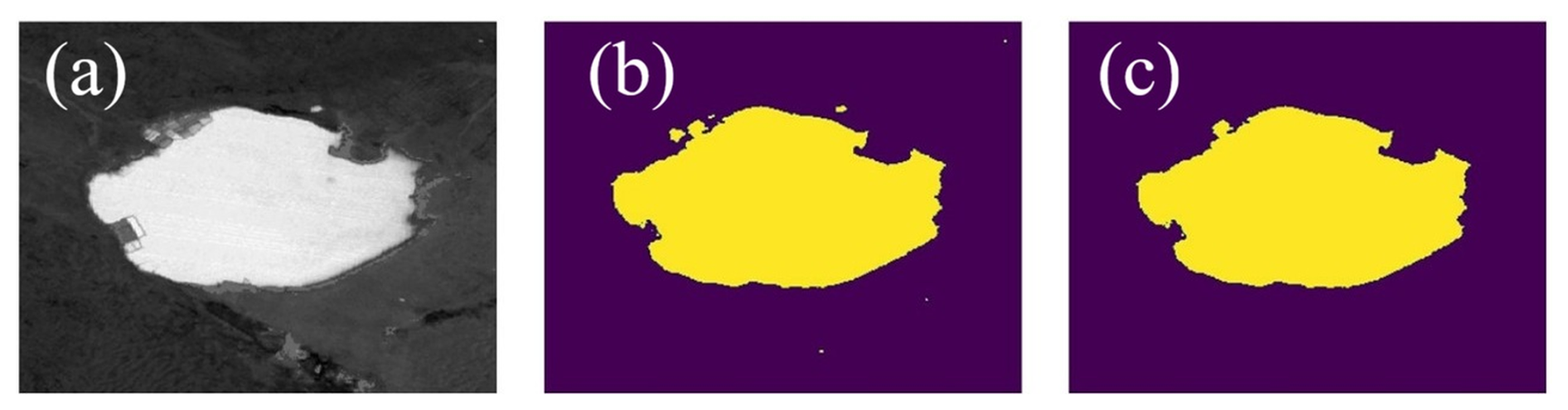
Figure 5 Illustration of water extraction and building removal processes. (a) Original Landsat image, in which white areas include both lake water and built-up surfaces; (b) water bodies extracted using threshold-based segmentation; (c) buildings separated from water bodies using the maximum connected component method. Source: Landsat imagery courtesy of the U.S. Geological Survey (USGS), processed and interpreted by the authors.

3.1.3 Cloudy and striped image reconstruction

1. Cloudy image filling processing. For cloud-free images, the subsequent water-extraction steps are applied directly. For cloudy images, cloud-free images are first used to reconstruct missing pixels, after which the same processing steps are executed.

   The filling approach is as follows: Based on the cloud coverage information (CLOUD_COVER), images with cloud cover less than or equal to 30 % (CLOUD_COVER ≤30 %) are classified as cloud-free images, while others are considered cloudy images. The formula is as follows:

   $$\begin{array}{}\text{(19)}& \begin{array}{l}\text{Cloudy Image}=\left\{\text{Image}\mathrm{|}{\mathrm{CLOUD}}_{\mathrm{COVER}}\le \mathrm{30}\mathit{\%}\right\}\\ \text{Cloud-Free Image}=\left\{\text{Image}\mathrm{|}{\mathrm{CLOUD}}_{\mathrm{COVER}}>\mathrm{30}\mathit{\%}\right\}\end{array}\end{array}$$

   Then, the Mutual Information (MI) algorithm is used to perform the most similar matching between the cloudy image and all cloud-free images. Next, the most similar image is combined with the original cloudy image through a union operation to obtain the filled cloudy image. Finally, the reconstructed images are processed using the same lake-extraction workflow as applied to cloud-free images, producing the final water-body area estimates:

   • Candidate Cloud-Free Image Set. In the time periods before and after the cloudy image, select images with low cloud coverage (CLOUD_COVER ≤30 %) as the candidate image set.

   • Mutual Information Algorithm. Use the MI algorithm to calculate the similarity between the cloudy image and the candidate cloud-free images. The formula is as follows:

     $$\begin{array}{}\text{(20)}& \begin{array}{rl}I(I_{\mathrm{cloudy}},I_{\mathrm{clear}})& =\sum _{i,j}p(I_{\mathrm{cloudy}}=i,I_{\mathrm{clear}}=j)\\ & \log \left({\displaystyle \frac{p(I_{\mathrm{cloudy}}=i,I_{\mathrm{clear}}=j)}{p(I_{\mathrm{cloudy}}=i),p(I_{\mathrm{clear}}=j)}}\right)\end{array}\end{array}$$

     Where I_cloudy represents the cloudy image, I_clear represents the candidate cloud-free image, and p is the joint probability distribution of the pixel grayscale values. III denotes mutual information, which measures the correlation between the cloudy image and the cloud-free image.

     Selecting the Most Similar Image: Based on the mutual information value, the cloud-free image most similar to the cloudy image is selected.

2. Striped image filling. The previously mentioned dataset indicates that Landsat 7 TM images have significant striping interference. Additionally, Landsat 5 TM and Landsat 8 OLI images also experience striping interference in certain months, such as Landsat 5 TM from 2001 to 2003 and Landsat 8 in 2008. To more accurately obtain the temporal changes in lake area, it is necessary to fill the missing portions of striped images. The method is the same as for cloud-filled images. By utilizing the clear contours of historical cloud-free images and applying the MI algorithm, the most similar historical cloud-free images are searched to fill the water pixels in the striped regions. The method for filling striped images is the same as that for cloud-filled images.

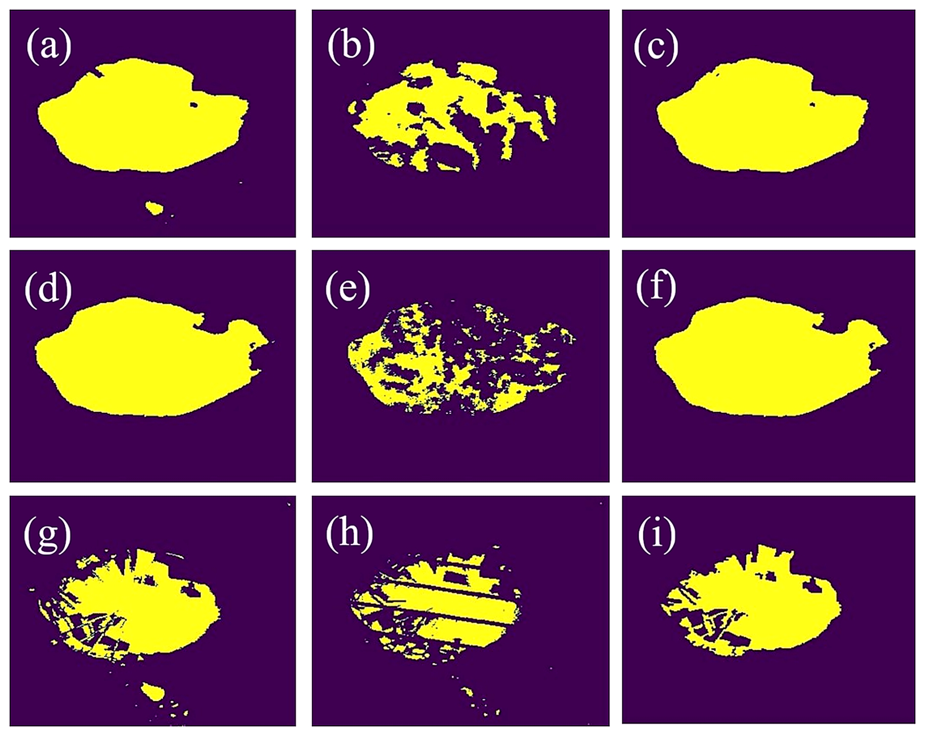
Figure 6 Filling processing of cloudy and striped-interference lake images using similar cloud-free references. (a, d) Cloud-free reference images identified as most similar to the cloudy images; (b, e) Original cloudy images; (c, f) Cloud-filled results after processing; (g) Cloud-free image most similar to the striped-interference image; (h) Original striped-interference image; (i) Result after stripe-filling processing. Source: Landsat imagery courtesy of the U.S. Geological Survey (USGS), processed and interpreted by the authors.

3.1.4 Monthly synthesis and time-series construction

After applying the maximum connectivity component processing to the image, the number of water pixels is counted. Then, based on the spatial resolution of the pixels (30 m × 30 m), the actual area is calculated.

Collect all known lake area data for specific time points, where t_i dots represent time points with available data. For each missing data point t_missing, use the known data points t_missing−1 and t_missing+1, and apply the selected interpolation method to calculate the lake area A(t_missing) at time.

3.2 Lake area time series construction

3.2.1 Monthly lake-area time series and seasonal variability of Bahannao Lake

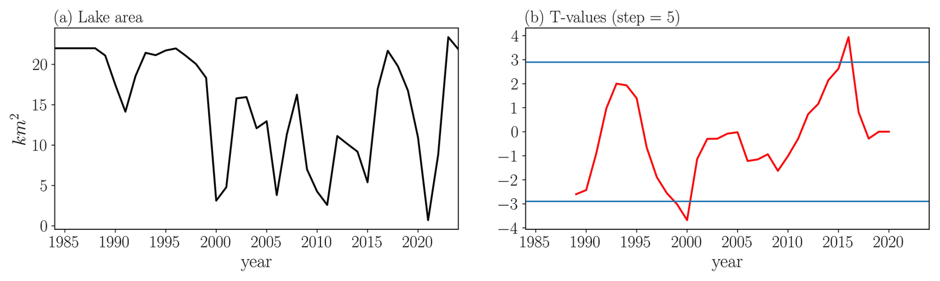
The interannual variation of Bahannao is quite drastic, but the overall trend is declining (Fig. 7a), linear regression analysis based on the year index reveals a significant declining trend in the lake area from 1984 to 2024, with a decrease rate of −0.29 km² yr⁻¹ (p=0.001). The coefficient of determination (R²=0.25) indicates substantial interannual variability, suggesting that although the long-term trend is statistically robust, short-term fluctuations and nonlinear processes play an important role in shaping lake-area dynamics. Before 1999, the changes were relatively stable. In 2000, the lake area shrank severely, decreasing by 82.98 % compared to 1999, leaving only 3.12 km². Since then, the lake has exhibited a cyclical fluctuation pattern with a period of approximately 5–6 years. In 2021, the lake area reached its minimum value of just 0.71 km², followed by a rapid increase, reaching its maximum of 23.38 km² in 2023.

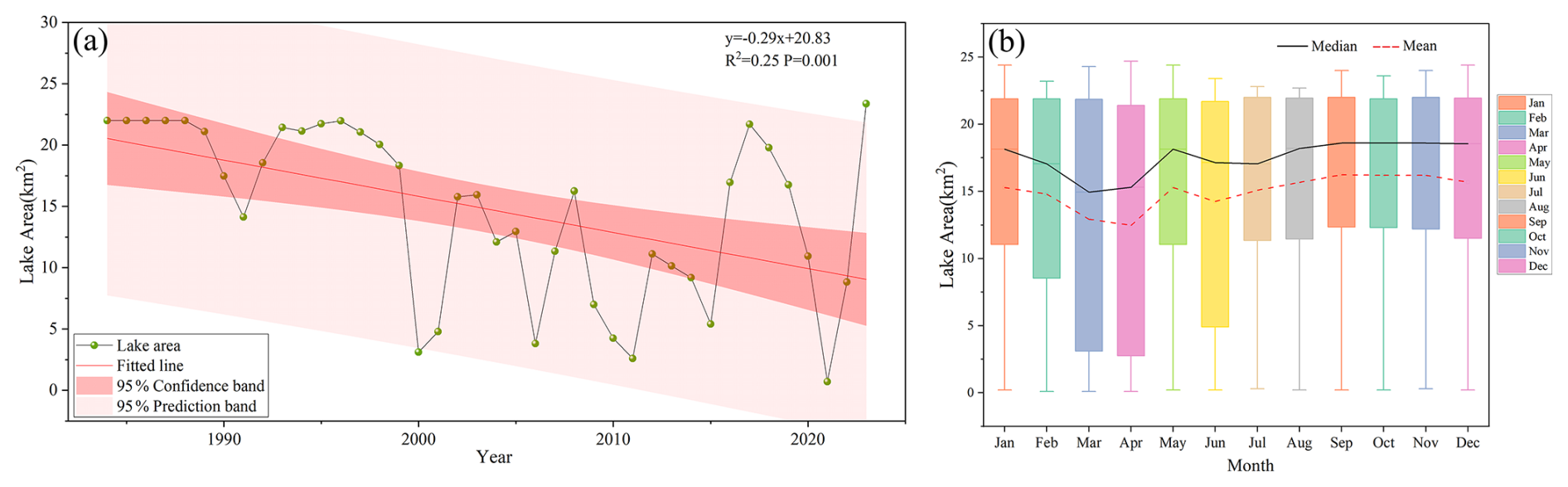
Figure 7 Interannual and intra-annual variation of Bahannao Lake area. (a) Interannual variations of lake area; (b) multi-year mean monthly variations of lake area.

Due to its location in the Mu Us Desert and the lack of long-term observational data, this study references the lake area interpreted via remote sensing in the Comprehensive Lake Water Ecological Management Plan of Uxin Banner. This report provides remote sensing imagery data for 24 years from 1988 to 2018 (with six years lacking clear images suitable for analysis).

A comparison of the data (Fig. 8a) shows that the lake area interpreted in this study aligns with the trend reported in the management plan. Over the 23 years of overlapping interpretation, the error remains within 15 % for 12 years. However, in years when the lake area was smaller, the error was relatively larger, such as in 2000, 2001, 2009, 2010, 2011, and 2015. According to records, Bahannao Lake shrank significantly during these years but did not completely dry up until 2021, which is consistent with the results of this study.

The interpreted lake area in this study also indicates (Fig. 8b) that the annual average area of Bahannao Lake in 2021 was only 0.71 km². The lake area was at its smallest in August, September, and October, reaching only 0.2 km², while the largest area was recorded in March at 3.5 km². The rapid expansion of the lake area observed in the spring of 2021 may be related to short-term hydrological inputs. Although the precipitation in this region during winter and early spring is generally limited, occasional short-term precipitation events or snowmelt may temporarily increase surface runoff and inflow to the lake. In addition, as temperatures rise in late spring, enhanced evaporation and reduced inflow may lead to a rapid decrease in lake area. Therefore, the rapid increase and subsequent decrease in lake area in spring 2021 may reflect the combined effects of short-term hydrological inputs and seasonal evaporation processes.

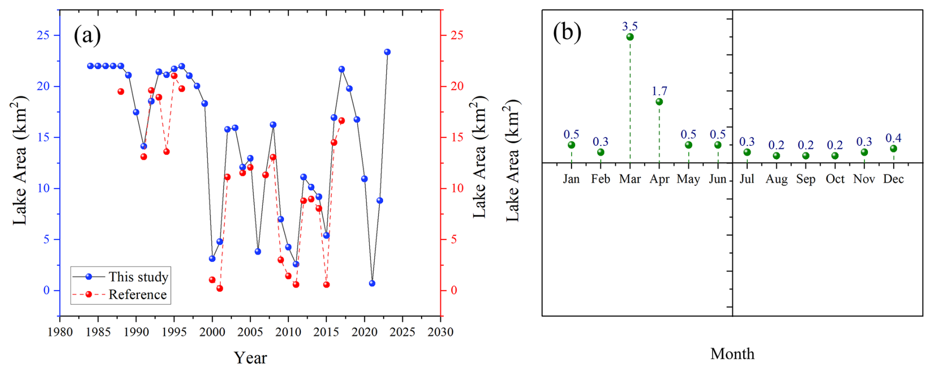
Figure 8 Validation of lake area estimates and intra-annual variability in a typical year (2021). (a) Comparison between lake area derived in this study and reference datasets; (b) monthly variations of lake area in 2021, selected as a representative year to illustrate intra-annual dynamics.

Figure 9 Seasonal variation of lake area during the period of 1984–2024.

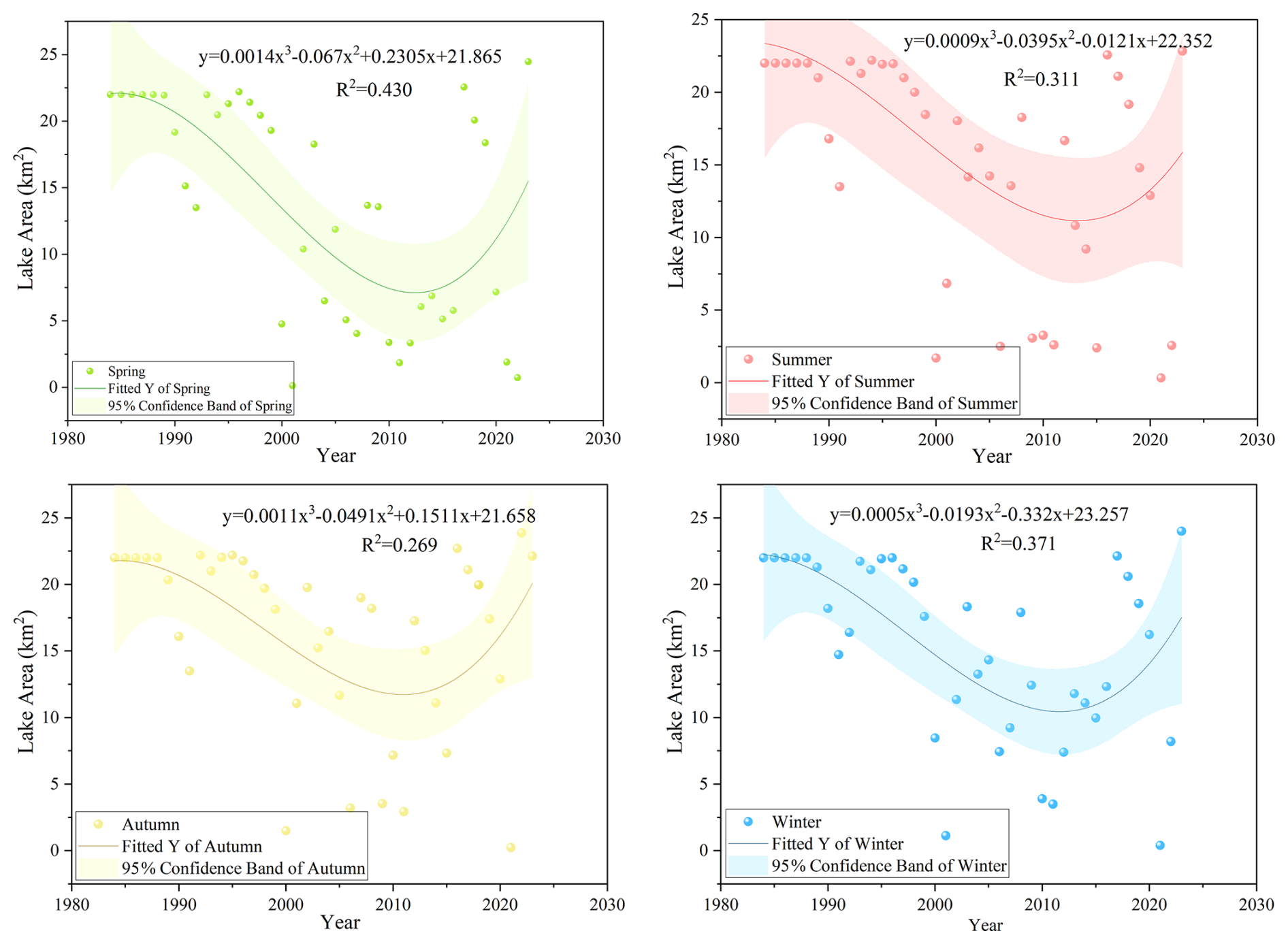
From the perspective of seasonal (Fig. 9) and monthly (Fig. 7b) variation characteristics, Bahannao exhibits significant seasonal differences. The lake area in summer, autumn, and winter is noticeably larger than in spring, with autumn having the largest lake area, averaging 16.21 km² and reaching a peak of 16.24 km² in September. In contrast, spring has the smallest lake area, averaging only 13.57 km², with the lowest value of 12.48 km² occurring in April.

3.2.2 Method validation using representative lakes in arid regions

To further evaluate the robustness and regional applicability of the proposed lake-area extraction method, we applied the same remote-sensing workflow to two representative lakes in arid and semi-arid northern China: Hongjiannao Lake and Wuliangsuhai Lake. These lakes differ markedly in size, hydrological conditions, and degree of human influence, and have been widely investigated in previous remote-sensing studies, providing independent reference datasets for method validation.

Using the identical image-processing procedures and water-body extraction criteria as those employed for Bahannao Lake, we constructed annual lake-area time series for both Hongjiannao Lake and Wuliangsuhai Lake (Fig. 10). The derived time series capture the major interannual fluctuations and long-term trends of lake-area variability for both lakes.

To quantitatively assess consistency with existing studies, the lake-area estimates obtained in this study were compared with previously published lake-area datasets (Fig. 11). For both lakes, the temporal evolution and long-term trends derived in this study show good agreement with reference datasets reported in the literature.

For Hongjiannao Lake, quantitative comparison indicates that the relative differences between lake-area estimates derived in this study and published datasets generally remain within a reasonable range. Specifically, the maximum and minimum relative differences are 14.65 % and 9.12 % when compared with Ji et al. (2023), 18.70 % and 9.57 % with Xie et al. (2021), 11.82 % and 8.29 % with Ma et al. (2020), 11.30 % and 7.94 % with Wang et al. (2018b), and 10.57 % and 3.15 % with Liu and Yue (2016).

For Wuliangsuhai Lake, the relative differences are generally smaller, with maximum differences of 8.50 % (minimum 1.74 %) compared with Guan (2022), 8.02 % (minimum 1.79 %) compared with Li et al. (2023), and 18.12 % (minimum 1.09 %) compared with Tan et al. (2021). These results indicate a high level of consistency between the lake-area estimates derived in this study and those reported in previous literature.

Although minor discrepancies in absolute lake-area values are observed, these differences can be attributed to variations in image selection, water-index thresholds, temporal coverage, and post-processing strategies among different studies. An additional source of discrepancy arises from differences in temporal aggregation strategies. In this study, annual lake area is calculated as the mean of monthly lake-area estimates derived from all available images within a year, which reduces the influence of short-term fluctuations and image-specific noise. In contrast, many previous studies report lake area based on a single image or a limited number of images selected for each year. Such differences in temporal representation can lead to systematic deviations in absolute lake-area values, particularly for lakes exhibiting strong intra-annual variability.

Overall, the consistency between our results and independent reference datasets supports the robustness and transferability of the proposed lake-area extraction method across different lake types in arid and semi-arid regions. This validation provides confidence that the method is suitable for long-term lake-area monitoring and comparative analysis in data-sparse dryland environments.

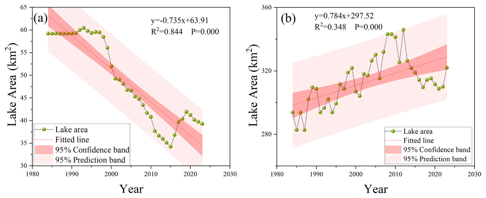
Figure 10 Interannual variations in lake area for Hongjiannao Lake (a) and Wuliangsuhai Lake (b).

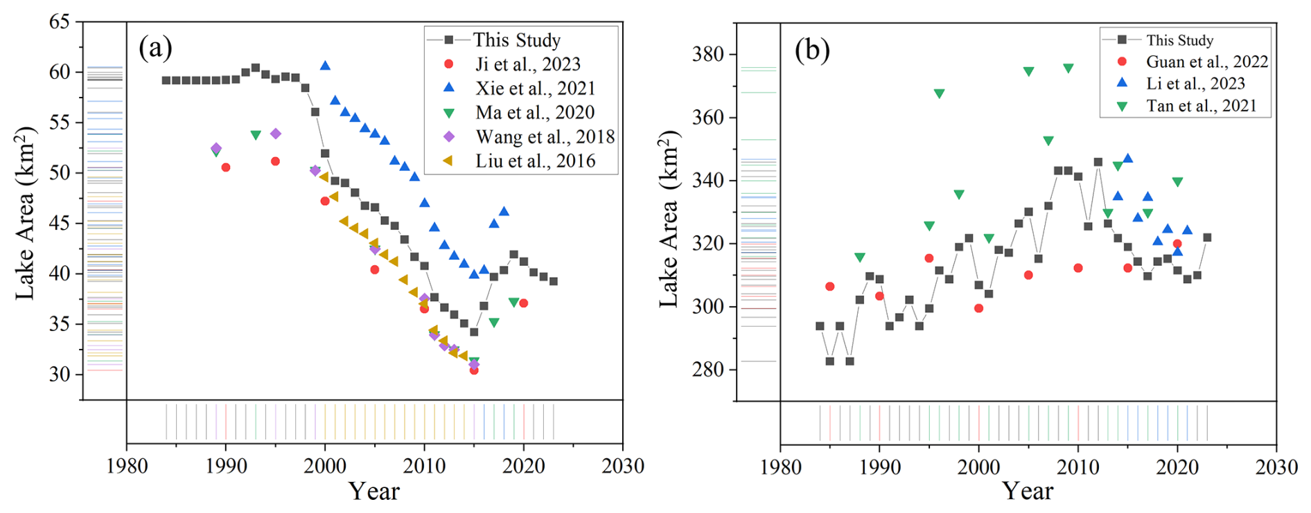
Figure 11 Comparison of lake area estimates derived in this study with published reference datasets. (a) Comparison of Hongjiannao Lake area with lake-area estimates reported in previous studies; (b) Comparison of Wuliangsuhai Lake area with lake-area estimates reported in previous studies.

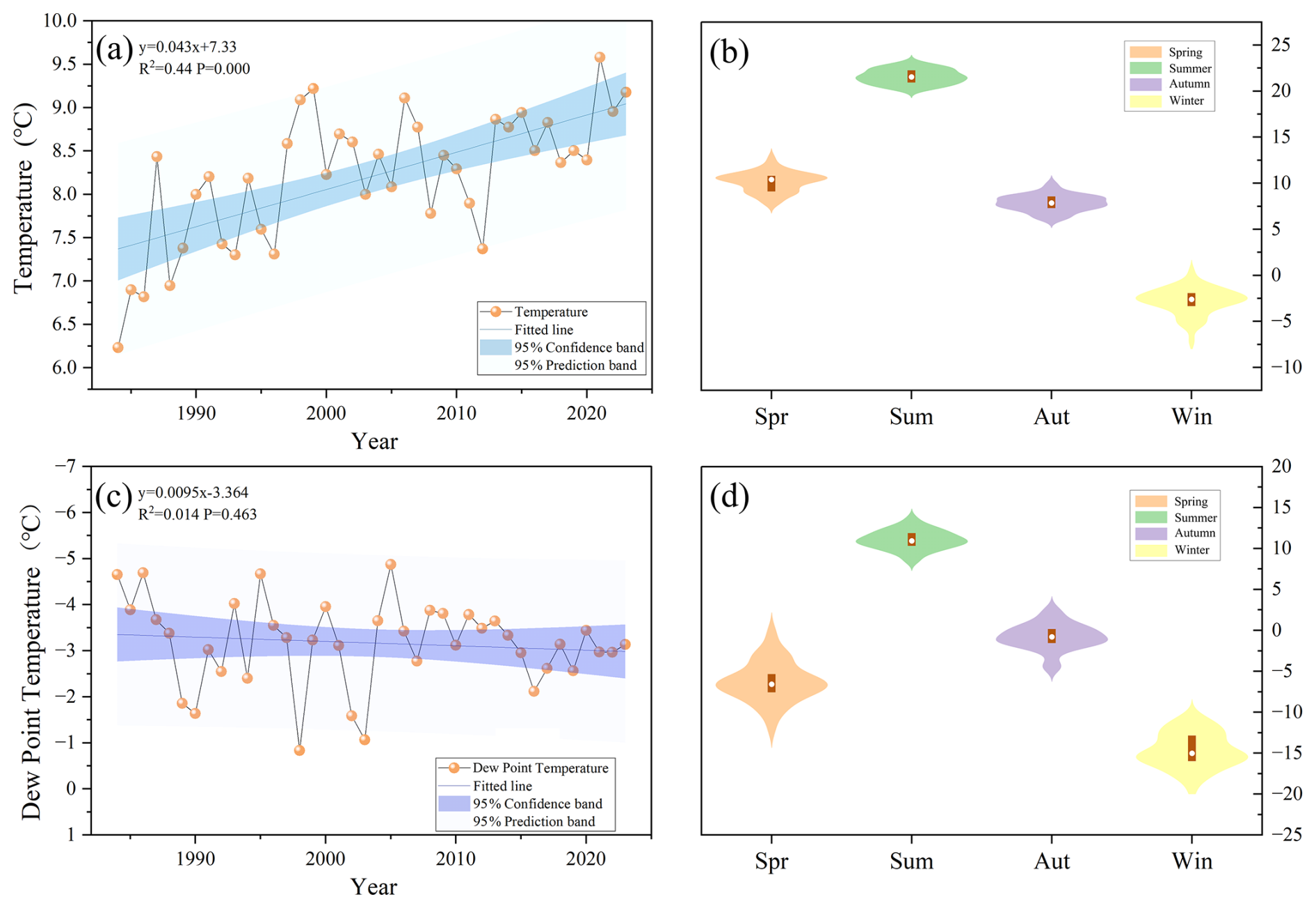
Figure 12 Temporal and seasonal variations in air temperature and 2 m dew point temperature over the study area during the period of 1984–2024. (a) Interannual variations in air temperature; (b) Multi-year mean seasonal cycle of air temperature; (c) Interannual variations in 2 m dew point temperature; (d) Multi-year mean seasonal cycle of 2 m dew point temperature.

3.3 Impact of climate change

3.3.1 Changes of hydro-climate series

• 1.

  Temperature and moisture conditions

  • a.

    Temperature and 2m dew point temperature. The rise in air temperature directly affects the evaporation rate of the lake. The warming rate is 0.043 °C yr⁻¹ (Fig. 12a), leading to an increase in the lake surface temperature and, consequently, higher evaporation. High temperatures intensify water evaporation, reducing the lake's water volume and causing a gradual decrease in lake area over the years.

    The increase in air temperature enhances heat input into the water body, accelerating evaporation. As more heat is absorbed, surface water transforms more easily into water vapor, leading to a decline in lake water levels. Although the influence of temperature on lake area varies across different time periods, its continuous upward trend has a long-term impact on the reduction of lake area.

    The 2 m dew point temperature increases at a rate of 0.0095 °C yr⁻¹ (Fig. 12c), indicating changes in atmospheric humidity. A rising dew point temperature suggests an increase in water vapor content in the air, typically associated with higher humidity. However, humidity changes do not always directly impact lake area; instead, they influence lake water volume indirectly by affecting evaporation and precipitation. While an increase in dew point temperature usually indicates higher humidity, if precipitation is insufficient or evaporation rates are too high, this increase in humidity may not effectively replenish lake water. Instead, it could contribute to lake shrinkage. The varying influence of the 2 m dew point temperature over different periods suggests a complex relationship with lake area changes, requiring a comprehensive analysis alongside other climatic factors.

  • b.

    Precipitation and relative humidity. The total precipitation is decreasing at a rate of 1.736 mm yr⁻¹ (Fig. 13a). Precipitation is one of the primary sources of lake water. A reduction in precipitation leads to insufficient water replenishment for the lake, resulting in a decline in water levels and a reduction in lake area.

    The relative humidity decreases at a rate of 0.099 yr⁻¹ (Fig. 13c). A decrease in humidity typically accelerates evaporation from the lake, leading to a reduction in lake area. The decrease in humidity means that the air becomes drier, and the evaporation rate increases. This accelerates the evaporation of lake water, resulting in a decline in both lake water levels and area, intensifying the process of lake desiccation.

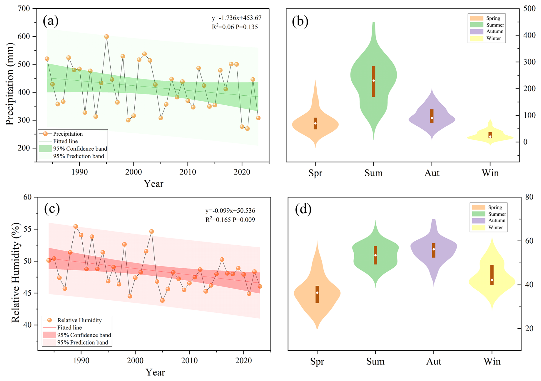
Figure 13 Temporal and seasonal variations in precipitation and relative humidity over the study area during the period of 1984–2024. (a) Interannual variations in precipitation; (b) Multi-year mean seasonal cycle of precipitation; (c) Interannual variations in relative humidity; (d) Multi-year mean seasonal cycle of relative humidity.

• 2.

  Surface radiation and heat flux components

  • a.

    Net longwave radiation and net shortwave radiation at the surface. Net longwave radiation at the surface decreases by 0.084 W m⁻² yr⁻¹ (Fig. 14a). The reduction in longwave radiation means that the lake receives less radiative heat, which theoretically could reduce evaporation. However, this effect is overshadowed by other factors such as reduced precipitation and rising temperatures. While the decrease in longwave radiation could reduce heat loss from the lake, in conditions of drought and high evaporation, the impact of this reduction is likely limited.

    Net shortwave radiation at the surface increases by 0.065 W m⁻² yr⁻¹ (Fig. 14a). The increase in shortwave radiation enhances the evaporation process, thereby reducing the lake's surface area. The rise in shortwave radiation leads to an increase in surface temperature, which accelerates evaporation. The intensified evaporation exacerbates the loss of water from the lake. The effect of increased shortwave radiation on the lake's area is significant during all periods, especially under drought and high-temperature conditions, where its impact is particularly pronounced.

  • b.

    Mean surface latent heat flux and sensible heat flux. The latent heat flux decreases at a rate of 0.081 W m⁻² yr⁻¹ (Fig. 14c). The decrease in latent heat flux indicates a reduction in the moisture carried by the air, possibly as a result of decreased humidity, which further intensifies evaporation from the water.

    The sensible heat flux increases by 0.095 W m⁻² yr⁻¹ (Fig. 14c), meaning that the heat exchange between the surface and the atmosphere is enhanced. This leads to more evaporation, particularly during the summer when temperatures are higher.

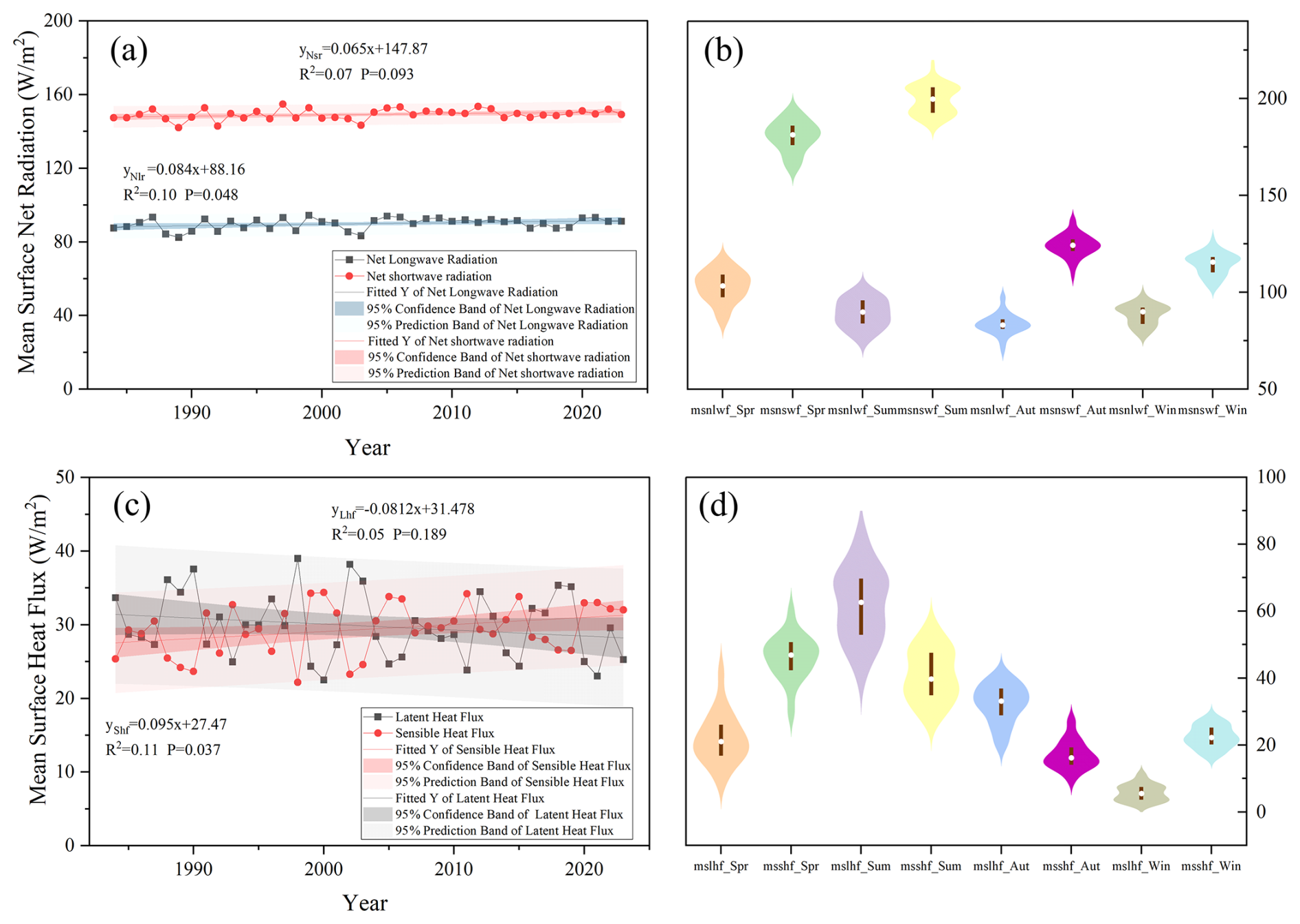
Figure 14 Regional variations of surface net radiation and surface heat flux during 1984–2024. (a) Interannual variations of mean surface net radiation; (b) multi-year mean seasonal variations of surface net radiation; (c) interannual variations of mean surface heat flux; (d) multi-year mean seasonal variations of surface heat flux. Abbreviations: msnlwf denotes mean surface net longwave radiation; msnswf denotes mean surface net shortwave radiation; mslhf denotes mean surface latent heat flux; msshf denotes mean surface sensible heat flux. The suffixes Spr, Sum, Aut, and Win represent spring, summer, autumn, and winter, respectively.

• 3.

  Evaporative demand and aridity conditions

  • a.

    Potential evapotranspiration. Potential evapotranspiration increases at a rate of 1.937 mm yr⁻¹ (Fig. 15a). The increase in evapotranspiration directly leads to the loss of water from the lake, making it an important factor contributing to the reduction in lake area. The rise in potential evapotranspiration indicates that both evaporation and plant transpiration in the lake area are increasing, further reducing the water volume of the lake. The increase in potential evapotranspiration has a significant impact on the lake area in all time periods, especially under drought and high-temperature conditions, where its effect is even more pronounced.

  • b.

    Drought. The aridity index (AI) exhibits pronounced interannual variability over the study period, with values generally fluctuating between approximately 0.18 and 0.40 (Fig. 15c), indicating persistently dry climatic conditions in the study area. Although a decreasing trend is observed (−0.0015 yr⁻¹), the trend is not statistically significant at the 0.05 level (p=0.07), suggesting that long-term aridity intensification is moderate rather than abrupt.

    Despite the weak linear trend, the consistently low AI values (<0.5) confirm that Bahannao Lake is located within a semi-arid to arid climatic regime, where water availability is inherently limited and highly sensitive to changes in hydro-climatic forcing. The wide prediction band further reflects strong year-to-year variability in regional moisture conditions, likely driven by fluctuations in precipitation and evaporative demand.

    Importantly, the combination of a marginally decreasing AI trend and a significant increase in potential evapotranspiration implies a gradual shift toward enhanced atmospheric water demand, even in the absence of a statistically significant drying trend in AI alone. This suggests that lake-area dynamics are more strongly controlled by evaporative processes than by precipitation-driven moisture supply, particularly in recent decades.

In addition to interannual variability, the aridity index (AI) exhibits pronounced seasonal contrasts (Fig. 15d). Summer shows the highest AI values, with a relatively wide distribution and higher median, indicating comparatively wetter conditions driven by concentrated precipitation during the warm season. Autumn presents intermediate AI values, reflecting a transition from moisture input to increasing evaporative demand.

In contrast, spring and winter are characterized by distinctly lower AI values. Spring exhibits low median AI and limited dispersion, indicating persistent moisture deficit during the lake recharge period. This seasonal dryness coincides with rising temperatures and increasing evaporative demand, which constrains lake expansion despite episodic precipitation events. Winter shows the lowest AI values overall, reflecting extremely dry atmospheric conditions dominated by minimal precipitation and suppressed moisture availability.

The seasonal pattern of AI highlights that Bahannao Lake is subject to strong intra-annual asymmetry in hydro-climatic conditions, with relatively favorable moisture supply confined to summer, while prolonged dry conditions prevail during spring and winter. Such seasonal dryness amplifies the sensitivity of lake area to evaporative processes.

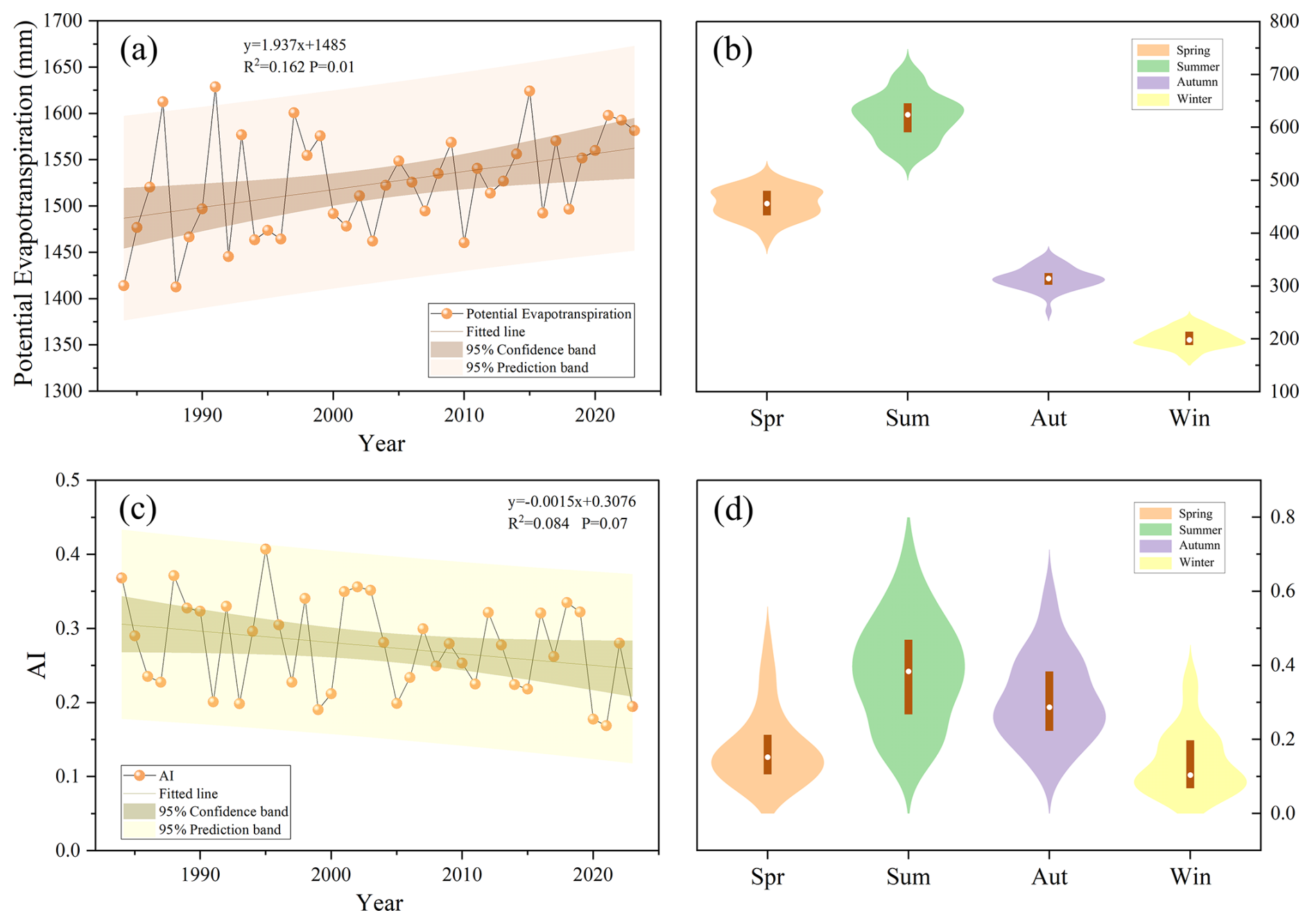
Figure 15 Regional variations in evaporation and drought conditions during 1984–2024. (a) Interannual variations of potential evapotranspiration; (b) multi-year mean seasonal variations of potential evapotranspiration; (c) interannual variations of the AI; (d) multi-year mean seasonal variations of the AI.

Figure 16 Time series and sliding T test of the area of the Bahannao Lake.

3.3.2 Impacts of hydro-climate elements on lake area

1. Linear relationships between lake area and climatic variables. A sliding T test on the lake area (Fig. 16) reveals two turning points in the lake's area change, specifically in 2000 and 2015. Therefore, we divide the study period into three time segments: the first period from January 1984 to December 1999, the second period from January 2000 to December 2014, and the third period from January 2015 to July 2024, to investigate the causes of the changes in lake area.

   The seasonal correlation analysis reveals pronounced differences in lake–climate relationships across seasons (Fig. 17a). In spring, lake area exhibits a significant positive correlation with relative humidity (RH) (r=0.403, p<0.01) and a significant negative correlation with temperature (T) ($r=-\mathrm{0.352}$, p<0.05), indicating that spring lake-area variability is sensitive to atmospheric moisture conditions and warming processes. In contrast, correlations with precipitation (P) and potential evapotranspiration (PET) are weak and not statistically significant.

   During summer, the lake–climate relationships are strongest. Lake area shows significant negative correlations with temperature ($r=-\mathrm{0.549}$, p<0.01) and PET ($r=-\mathrm{0.315}$, p<0.05), and significant positive correlations with precipitation (r=0.437, p<0.01) and RH (r=0.468, p<0.01). These results indicate that summer lake-area variability is jointly controlled by moisture supply and enhanced evaporative demand.

   In autumn, lake area is significantly negatively correlated only with temperature ($r=-\mathrm{0.315}$, p<0.05), whereas correlations with precipitation, RH, and PET are not significant, suggesting that autumn lake-area variations may reflect cumulative effects of antecedent hydro-climatic conditions. In winter, lake area shows a significant positive correlation with RH (r=0.315, p<0.05), while correlations with other climatic variables remain weak, reflecting reduced hydrological activity during the cold season.

   At the interdecadal scale, lake–climate correlations exhibit clear stage-dependent characteristics (Fig. 17b). During the period 1984–1999, lake area shows no significant correlation with temperature, precipitation, PET, or RH, indicating a relatively weak response to individual climatic factors.

   During 2000–2014, lake area becomes significantly positively correlated with precipitation (p<0.05) and RH (p<0.01), suggesting an enhanced sensitivity of lake-area variability to moisture conditions during this period. In the most recent period (2015–2024), lake area maintains a significant positive correlation only with RH (p<0.05), while correlations with other climatic variables weaken, implying a dominant role of atmospheric moisture conditions in regulating recent lake-area changes.

2. Nonlinear hydro-climatic controls revealed by XGBoost. To further quantify the relative importance of climatic variables and explore potential nonlinear effects beyond linear correlations, an XGBoost model was applied using precipitation, temperature, relative humidity, and potential evapotranspiration as predictors.

   Model evaluation indicates that training performance generally exceeds testing performance, and testing R² values are relatively low or even negative in some cases. This behavior reflects the limited sample size, strong interannual variability, and inherent nonlinearity of lake-area dynamics in arid regions, rather than model inadequacy. Therefore, in this study, XGBoost is primarily used as an interpretative tool to assess the relative importance of climatic drivers rather than as a predictive model.

   XGBoost-derived feature importance exhibits clear seasonal contrasts that broadly agree with the correlation analysis while providing additional insights into nonlinear controls (Fig. 18a). In spring, XGBoost feature importance indicates that air temperature is the most influential predictor (T, 0.31), followed by relative humidity (RH, 0.28), whereas precipitation (P, 0.20) and potential evapotranspiration (PET, 0.20) play secondary roles. This finding is consistent with the correlation analysis, which shows a significant positive correlation between lake area and RH (r=0.403, p<0.01) and a significant negative correlation with air temperature ($r=-\mathrm{0.352}$, p<0.05). Together, these results highlight the sensitivity of springtime lake dynamics to atmospheric moisture conditions and evaporative demand. Long-term trend analysis further indicates a significant increase in air temperature at a rate of 0.043 °C yr⁻¹ (p<0.001) and a significant decline in RH (−0.099 yr⁻¹, p=0.009), reinforcing the role of enhanced evaporation and atmospheric drying in shaping spring lake-area changes.

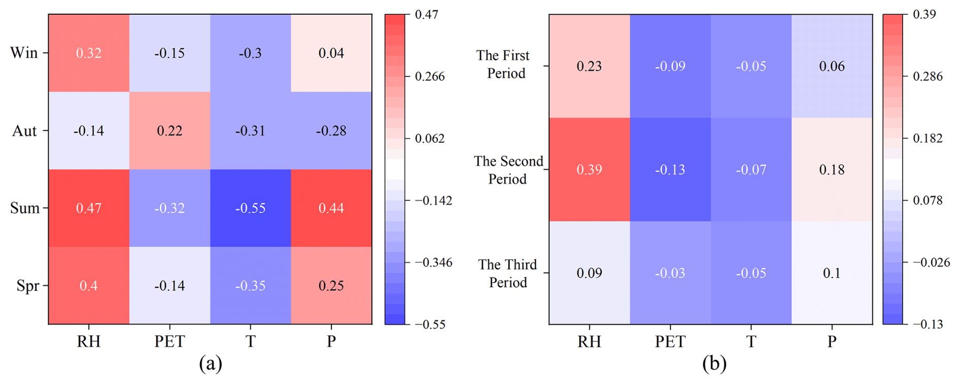
Figure 17 Seasonal and interdecadal differences in correlations between lake area and climatic drivers. (a) Seasonal correlations between lake area and RH, PET, T, and P. (b) Correlations between lake area and climatic variables across three sub-periods (1984–1999, 2000–2014, and 2015–2024).

In summer, air temperature (T, 0.35) and relative humidity (RH, 0.26) dominate the feature-importance rankings, with precipitation (P, 0.18) and potential evapotranspiration (PET, 0.21) also contributing substantially. This aligns well with the correlation results, which indicate that summer lake area is positively correlated with precipitation (r=0.437, p<0.01) and RH (r=0.468, p<0.01), and negatively correlated with temperature ($r=-\mathrm{0.549}$, p<0.01) and PET ($r=-\mathrm{0.315}$, p<0.05). Trend analysis shows that although precipitation exhibits a decreasing tendency (−1.736 mm yr⁻¹, p=0.135, not significant), PET increases significantly at a rate of 1.937 mm yr⁻¹ (p=0.01). This suggests that summer lake-area variability is increasingly constrained by enhanced evaporative demand, with the balance between water input and evaporation losses playing a dominant role.

In autumn, linear correlations between lake area and most climatic variables are weak and statistically insignificant. However, XGBoost results still indicate relatively high importance for relative humidity (RH, 0.34) and potential evapotranspiration (PET, 0.31), suggesting that autumn lake dynamics may be governed by nonlinear processes or threshold effects that are not adequately captured by linear methods alone. Considering the significant upward trend in PET and the declining tendency of the aridity index (AI; −0.015 yr⁻¹, p=0.07), autumn lake systems appear to be transitioning toward evaporation-dominated control.

In winter, overall feature importance values are relatively low due to reduced hydrological activity, yet relative humidity (RH, 0.34) remains the most influential variable in the XGBoost model. This is consistent with the correlation analysis showing a significant positive relationship between winter lake area and RH (r=0.315, p<0.05), indicating that background atmospheric moisture conditions still serve as an important indicator of lake variability during the frozen period.

At the decadal scale, XGBoost results reveal a clear temporal shift in the dominant climatic controls on lake-area variability, as shown in Fig. 18b. During 1984–1999, the importance of individual climatic variables is generally low and dispersed, consistent with the weak correlations observed during this period. This suggests that the lake system exhibited relatively low sensitivity to climatic fluctuations in the early stage.

During 2000–2014, precipitation (P, 0.22), potential evapotranspiration (PET, 0.23) and relative humidity (RH, 0.34) show markedly higher importance in the XGBoost model, in agreement with correlation results indicating significant positive relationships between lake area and precipitation (r=0.179, p<0.05) and RH (r=0.388, p<0.01). This period is therefore characterized by a precipitation- and moisture-dominated control regime.

In the most recent period (2015–2024), the importance of temperature and PET increases noticeably, while the contribution of precipitation weakens. Combined with the observed warming trend and enhanced evaporative demand, these results indicate a transition toward an evaporation-dominated climatic control on lake-area dynamics in recent years.

By integrating long-term trend analysis, linear correlation analysis, and XGBoost-based nonlinear feature importance, this study demonstrates that lake-area variability in arid regions is not governed by a single climatic factor, but rather by the interplay between water supply and evaporative demand across different seasons and time scales. Linear correlation analysis effectively captures the summer lake–climate relationship dominated by water balance, whereas the nonlinear XGBoost approach provides complementary insights into more complex control mechanisms during transitional seasons such as spring and autumn. Overall, the results indicate that with continued regional warming, increasing PET, and intensifying aridity, evaporative processes are playing an increasingly important role in controlling lake-area variability, offering important implications for understanding the response of arid-region lakes to future climate change.

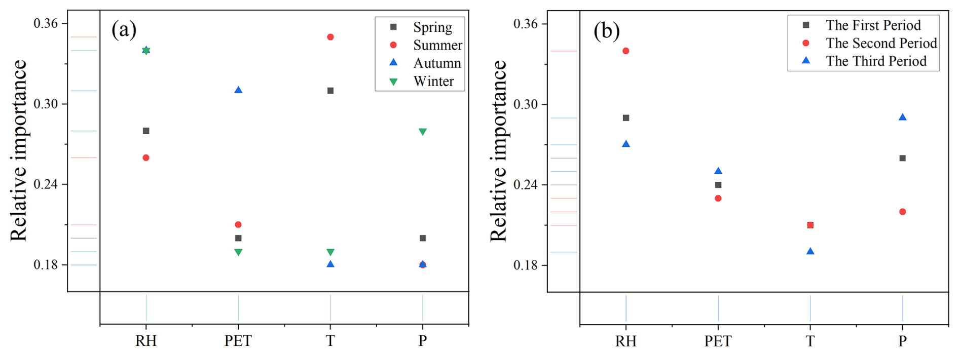
Figure 18 Weight of influencing factors by season. Abbreviations: RH denotes relative humidity (%); PET denotes potential evapotranspiration (mm); T denotes air temperature (°C); P denotes precipitation (mm).

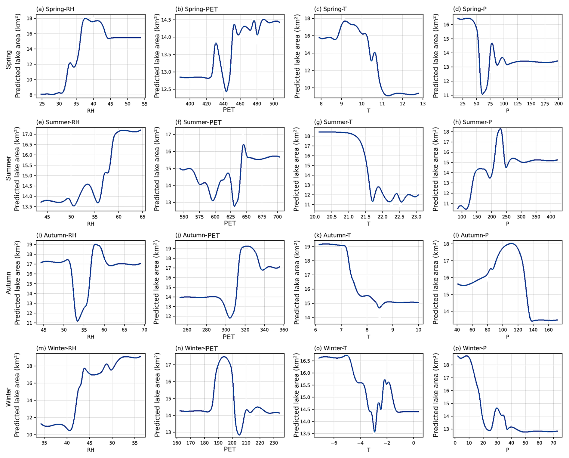
To further investigate the nonlinear relationships between lake area and climatic factors, partial dependence plots (PDPs) were generated for each season and period. The seasonal partial dependence plots (Fig. 19a–p) reveal pronounced seasonal differences and nonlinear responses of lake area to hydro-climatic variables.

In spring, lake area exhibits a clear threshold response to relative humidity (RH). When RH remains below approximately 34 %–35 %, the lake area shows only minor variation. However, when RH increases to around 38 %–40 %, the lake area rises rapidly, indicating that enhanced atmospheric moisture conditions can significantly support lake water storage. In contrast, PET shows a weak negative influence on lake area, while temperature exhibits a marked decline in lake area when it approaches approximately 10–11 °C, suggesting that intensified evaporation may suppress lake expansion. Precipitation shows only a limited influence, implying that spring lake dynamics are primarily controlled by atmospheric moisture conditions and evaporative demand.

During summer, precipitation demonstrates a pronounced nonlinear positive effect on lake area. When precipitation increases to approximately 200 mm, lake area expands rapidly, indicating that rainfall represents a major water input supporting lake expansion in the warm season. Relative humidity also shows a generally positive relationship with lake area, whereas increasing temperature leads to a clear decline in lake area, reflecting the strong evaporative effects under high-temperature conditions.

In autumn, lake area responds strongly to variations in PET, displaying a distinct nonlinear pattern. When ET0 approaches approximately 300 mm, lake area decreases sharply, whereas at higher PET levels the lake area shows partial recovery, suggesting a complex regulatory role of evaporative demand on lake water balance. Meanwhile, increasing temperature generally leads to a decline in lake area, highlighting the importance of evaporation processes in controlling autumn lake dynamics.

In winter, RH exhibits a strong positive effect on lake area. When RH increases from approximately 40 % to 50 %, lake area increases markedly, indicating that atmospheric moisture conditions play a key role in regulating winter lake variability. Precipitation exerts a relatively weak influence, while temperature variations mainly affect lake dynamics indirectly through their influence on evaporation processes.

Overall, these results demonstrate that the response of lake area to hydro-climatic variables is highly nonlinear and strongly season-dependent, with atmospheric moisture dominating in spring and winter, precipitation controlling summer expansion, and evaporative demand exerting a stronger influence during autumn.

Figure 19 Seasonal partial dependence plots (PDPs) derived from the XGBoost model.

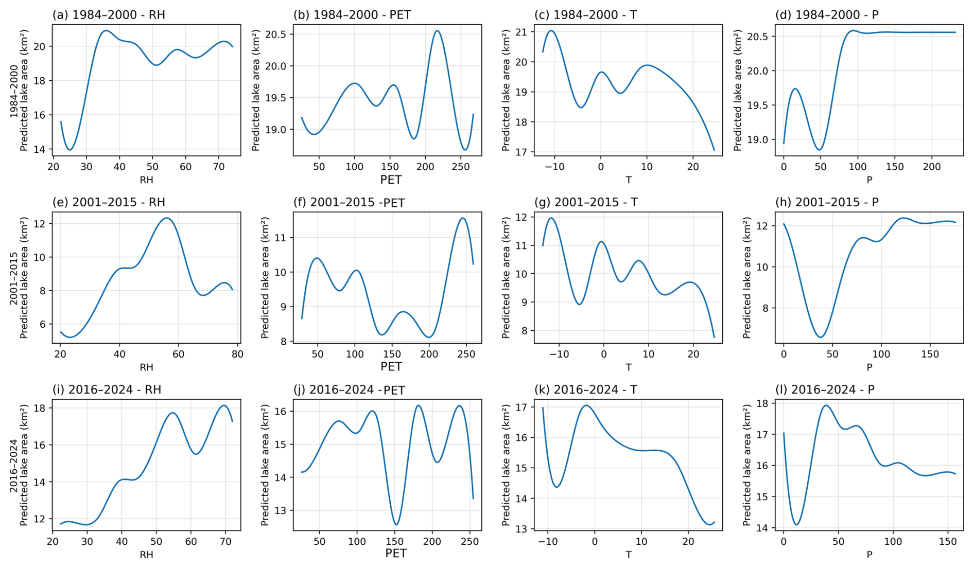
The partial dependence plots across the three periods (Fig. 20a–l) further reveal a clear temporal evolution in the hydro-climatic controls on lake area. During the first period, lake area shows a strong positive response to relative humidity (RH). When RH increases from approximately 30 % to around 40 %, lake area expands rapidly, indicating that atmospheric moisture conditions play a key role in sustaining lake water storage. Precipitation also exhibits a positive influence on lake area, particularly when precipitation exceeds approximately 80–100 mm, suggesting that water supply conditions were an important driver of lake expansion during this stage. In contrast, PET and temperature show relatively weaker influences, indicating that evaporative demand played a less dominant role during the early period.

In the second period, the nonlinear responses of lake area become more complex. RH still exerts a noticeable influence on lake area, but the relationship becomes less monotonic compared with the earlier stage. Meanwhile, the influence of PET becomes more evident, suggesting that evaporative demand began to exert a stronger regulatory effect on lake dynamics. Precipitation continues to show a positive relationship with lake area, although the magnitude of the response is slightly reduced, indicating a gradual shift from water-supply dominance toward a combined influence of water supply and evaporation processes.

During the most recent period, the PDPs indicate that temperature and PET exert stronger impacts on lake area variability. Increasing temperature generally leads to a decline in lake area, reflecting enhanced evaporation under warming climatic conditions. Similarly, higher PET values correspond to reduced lake area, indicating that evaporative demand has become an increasingly important control on lake dynamics. In contrast, the influence of precipitation becomes relatively weaker compared with earlier periods, suggesting that the hydrological sensitivity of the lake has gradually shifted toward stronger evaporation-driven regulation.

Overall, the PDP analysis across the three periods suggests a gradual transition in the dominant hydro-climatic controls on Bahannao Lake, shifting from moisture-supply-dominated processes in the early period toward stronger regulation by evaporative demand under recent warming conditions.

These results highlight that lake dynamics in Bahannao Lake are governed by complex nonlinear hydro-climatic interactions, and that the dominant climatic controls have evolved over time.

Figure 20 PDPs of hydro-climatic variables across three periods.

4 Discussion

This study constructed a continuous monthly lake-area time series for Bahannao Lake spanning 1984–2024 using an optimized lake-area extraction framework that integrates seasonal water-index selection, adaptive thresholding, maximum connectivity analysis, and mutual information–based gap filling. Compared with widely used long-term products such as the JRC Global Surface Water dataset, which are often constrained by cloud contamination, seasonal ice cover, and temporal discontinuities, the proposed framework substantially improves temporal continuity and robustness under complex environmental conditions. This improvement is particularly important for small lakes in arid and semi-arid regions, where data gaps and seasonal disturbances are pervasive in existing datasets.

At the methodological level, this study introduces targeted improvements at several critical steps relative to previous approaches. First, the seasonal application of NDWI and MNDSI for non-freezing and freezing periods, respectively, enhances the stability of water-body identification under varying surface conditions, outperforming traditional single-index methods (McFeeters, 1996; Yao et al., 2015). Second, the combination of Otsu thresholding with DEM-based terrain constraints effectively reduces misclassification caused by topographic shadows and complex terrain, which is a common challenge for inland lakes in arid environments. Third, the mutual information–based image-filling strategy reconstructs cloud- and stripe-contaminated pixels by matching historically most similar cloud-free images, thereby extending the usability of long-term Landsat archives. Compared with approaches relying solely on interpolation (Zhao and Gao, 2018), this strategy substantially improves the completeness and reliability of multi-decadal lake-area records. Collectively, these methodological enhancements systematically address key challenges repeatedly identified in previous studies, including cloud contamination, seasonal variability, topographic interference, and spectral complexity of inland waters (Mouw et al., 2015; Palmer et al., 2015; Shen et al., 2017; Cao et al., 2019), and establish a transferable framework suitable for lake monitoring in arid and data-scarce regions.

From a hydro-climatic perspective, the reconstructed long-term record provides important insights into the mechanisms controlling lake dynamics in arid environments. Consistent with previous studies, precipitation and evaporation emerge as the primary factors regulating lake-area variability, particularly during the warm season when both water inputs and evaporative losses are enhanced (Tao et al., 2015; Li et al., 2017). The correlation analysis indicates that lake area is significantly positively correlated with precipitation and relative humidity in summer, whereas atmospheric moisture conditions exert a more pronounced influence during spring and winter. These findings reinforce the view that lake dynamics in arid regions are governed by the seasonal balance between water supply and evaporative demand.

However, compared with many existing studies that rely primarily on annual-scale analyses, the monthly lake-area time series developed here reveals pronounced seasonal heterogeneity and transitional behavior. In spring and autumn, linear correlations between lake area and individual climatic variables are generally weak, whereas XGBoost feature-importance analysis consistently identifies relative humidity and potential evapotranspiration as influential factors. This discrepancy suggests that lake responses during transitional seasons may be governed by nonlinear processes or threshold effects that cannot be fully captured by linear statistical methods alone. The combined use of correlation analysis and XGBoost therefore provides complementary perspectives on lake–climate relationships across different temporal scales.

At the decadal scale, both correlation analysis and XGBoost results indicate a clear evolution in dominant climatic controls on lake-area variability. During 2000–2014, precipitation and relative humidity exhibit increased importance and significant positive associations with lake area, indicating a moisture-dominated control regime. In contrast, during 2015–2024, the importance of air temperature and potential evapotranspiration increases markedly, while the contribution of precipitation weakens. This shift reflects a transition toward evaporation-dominated control under sustained warming conditions and highlights a dynamic reorganization of hydro-climatic drivers. Such temporal evolution extends existing understanding by explicitly demonstrating how dominant controls on arid-region lakes can shift under intensified climate variability.

These results have broader implications for studies of lakes in arid and semi-arid regions. The fragile water balance and limited buffering capacity of dryland lakes render them highly sensitive to even modest changes in precipitation, atmospheric moisture, and evaporative demand. The observed transition from precipitation-dominated to evaporation-dominated control suggests increasing vulnerability of arid-region lakes under ongoing climate warming. Even in the absence of a pronounced decline in precipitation, enhanced evaporation and atmospheric drying may offset or exceed water inputs, thereby accelerating lake shrinkage. This finding underscores the necessity of considering multiple hydro-climatic factors simultaneously when assessing future lake trajectories in arid environments.

From a water-resources management perspective, the results indicate that lake conservation and management strategies in arid regions should not focus solely on precipitation trends but must also account for changes in evaporative demand, drought intensity, and atmospheric moisture conditions. The lake-area extraction framework and the insights into evolving climatic controls presented here provide a robust technical foundation for long-term lake monitoring, risk assessment, and adaptive water-management strategies in data-sparse dryland regions.

Several limitations of this study should be acknowledged. First, while remote sensing reliably captures surface-area dynamics, subsurface processes such as groundwater inflow and outflow were not explicitly quantified and may influence lake water balance. The relatively weak correlation between lake area and precipitation observed in this study further suggests that additional hydrological processes, such as groundwater exchange or delayed runoff responses, may contribute to lake-area variability in this semi-arid environment. However, due to the lack of long-term groundwater observations in the study area, these processes could not be directly evaluated in the present study. Second, the 30 m spatial resolution of Landsat data limits detection of fine-scale shoreline changes, and future studies could benefit from integrating higher-resolution sensors such as Sentinel-2. Third, although XGBoost effectively captures nonlinear relationships, its data-driven nature limits physical interpretability relative to process-based hydrological models. Future research could integrate remote sensing, machine learning, ecohydrological modeling, and socioeconomic data to further advance understanding of lake dynamics in arid regions.

5 Conclusion

This study developed an optimized remote-sensing framework to construct a continuous monthly lake-area time series for Bahannao Lake from 1984 to 2024. By integrating seasonal water-index selection, adaptive thresholding, connectivity analysis, and mutual information-based image reconstruction, the proposed method effectively overcomes common limitations associated with cloud contamination, seasonal ice cover, and data gaps in long-term Landsat archives. Validation using Hongjiannao Lake and Wuliangsuhai Lake further demonstrates the robustness and regional applicability of the framework for lake monitoring in arid and semi-arid environments.

The reconstructed time series reveals pronounced interannual variability and strong seasonal contrasts in lake-area dynamics. Linear correlation analysis indicates that lake-area variations are primarily associated with precipitation and atmospheric moisture conditions during the warm season, whereas evaporative demand plays an increasingly important role during cold and transitional seasons. The combined use of correlation analysis and XGBoost modeling further reveals a clear stage-dependent evolution of climatic controls. During 1984–1999, lake dynamics were mainly associated with humidity and precipitation variability; during 2000–2014, the influence of moisture-related conditions remained important under enhanced climate variability; and during 2015–2024, rising air temperature and potential evapotranspiration emerged as dominant contributors, indicating a transition toward evaporation-dominated control under sustained warming.

Overall, the results demonstrate that lake-area changes in arid regions are governed by nonlinear and evolving interactions between water supply and evaporative demand rather than by any single climatic factor. By combining high-temporal-resolution lake-area reconstruction with both linear and nonlinear analytical approaches, this study provides new insights into the mechanisms underlying arid-region lake dynamics. The proposed framework offers a valuable tool for long-term lake monitoring and contributes to improved understanding of eco-hydrological responses and water-resource vulnerability under ongoing climate change in dryland regions.