Technical note: Including non-evaporative fluxes enhances the accuracy of isotope-based soil evaporation estimates

Accurately estimating soil water evaporation is essential for quantifying terrestrial water and energy fluxes. Isotope-based methods are useful but often rely on steady-state (SS) soil water storage assumptions or non-steady-state (NSS) models that ignore non-evaporative fluxes (such as infiltration and transpiration), leading to mass balance errors. Here, we introduce a new framework, named ISONEVA (ISOtope based soil water evaporation estimation considers dynamic soil water storage and Non-EVAporative fluxes), adapted from lake evaporation models to account for both evaporative and non-evaporative fluxes in soils under dynamic soil water storage. Validation under virtual and field scenarios demonstrated that ISONEVA improved evaporation estimates by 24.2 %–79.0 % (virtual) and 57.1 %–79.0 % (field) compared to traditional SS and NSS methods. Furthermore, ISONEVA estimated a plausible upper limit of the $E/\mathrm{ET}$ ratio (0.15) in the field test, encompassing the observed value (0.126), whereas SS severely underestimated (0.02) and NSS is unable to estimate $E/\mathrm{ET}$. These results highlight the critical role of dynamic soil water storage and non-evaporative fluxes in isotope-based soil water evaporation estimates.

1 Introduction

Evaporation is a fundamental component of the water and energy balance, consuming nearly one-quarter of incoming solar energy and playing a critical role in land-atmosphere interactions (Or et al., 2013; Trenberth et al., 2009). The long-term (decades) ratio of soil water evaporation (from here onward, simply termed as soil evaporation) to precipitation ($E/P$) provides key insights into ecohydrological processes, supports accurate water balance assessments, informs evapotranspiration (ET) partitioning, and improves hydrological model calibration (Benettin et al., 2021; Kool et al., 2014; Vereecken et al., 2016).

Hydrogen and oxygen stable isotopes have emerged as a powerful tool to directly estimate soil evaporation by tracing the enrichment in heavy isotopes (δ²H and δ¹⁸O) in topsoil layers caused by evaporation-driven fractionation (Bailey et al., 2018; Rothfuss et al., 2021). Soil water evaporation and resulting isotope fractionation are highly transient due to dynamic solar radiation, wind speed and other meteorological factors. However, current isotope-based approaches rely on either steady-state (SS) or non-steady-state (NSS) frameworks. SS assumes constant soil water storage and isotopic composition over time, a condition rarely met in dynamic soil systems (Al-Oqaili et al., 2020; Xiang et al., 2021), yet its core assumption of constant water volume is only valid for large water bodies. NSS accounts for temporal variations in storage and isotopes but accounts only for evaporative fluxes (Gibson and Reid, 2010), neglecting subsurface flow (such as infiltration, root water uptake fluxes, and drainage), which can lead to biased estimates of evaporation (Mattei et al., 2020; Yidana et al., 2016). For example, some studies using NSS methods reported higher evaporation in forest sites compared to shrublands under similar meteorological conditions (Sprenger et al., 2017), contrasting the expectation that shrublands should exhibit greater soil evaporation due to more exposed soil and less canopy cover than forest (Benettin et al., 2021; Nicholls et al., 2023; Nicholls and Carey, 2021; Yu et al., 2022).

This discrepancy may reflect the influence of additional processes not fully accounted for in NSS methods, emphasizing the importance of explicitly representing non-evaporative fluxes, such as percolation and root water uptake, to ensure soil water and isotope mass balance when modelling soil evaporation. To address these limitations, we developed a new framework named ISONEVA (ISOtope based soil water evaporation estimation considers dynamic soil water storage and Non-EVAporative fluxes), extending the formulations originally derived for open water bodies (Gonfiantini, 1986). ISONEVA explicitly incorporates both evaporative and non-evaporative fluxes in the topsoil layer, offering a more realistic representation of soil processes and better soil water and isotope mass balance.

ISONEVA method is evaluated through a combination of virtual test and field lysimeter data, directly comparing it with SS and NSS approaches. By overcoming key theoretical and practical limitations of existing methods, ISONEVA has the potential to be a promising tool for advancing soil evaporation assessments in diverse ecosystems and supports improved water resource management under climate change. This study begins by outlining the theoretical basis of the ISONEVA framework and then evaluates its performance through a combination of virtual and field datasets. The objective is to explore the method's advantages, limitations, and its broader applicability in isotope-based hydrological studies.

2 Material and Methods

2.1 Method derivatives

A coordinate system is established with the zero-flux plane positioned at the soil surface, and the downward direction defined as positive. Within this framework, fluxes in the topsoil layer include precipitation (P), evaporation (E), and percolation (Q). P and E have positive and negative directions, respectively; while the direction of Q depends on the balance between P and E: when E exceeds P over a given period, Q can be negative; conversely, when P exceeds E, Q is typically positive (Fig. 1). Note that Q can be interpreted more broadly as the sum of all non-evaporative fluxes (do not result in significant isotopic fractionation) that leave the topsoil layer (positive sign), such as percolation and root water uptake (Fu et al., 2025).

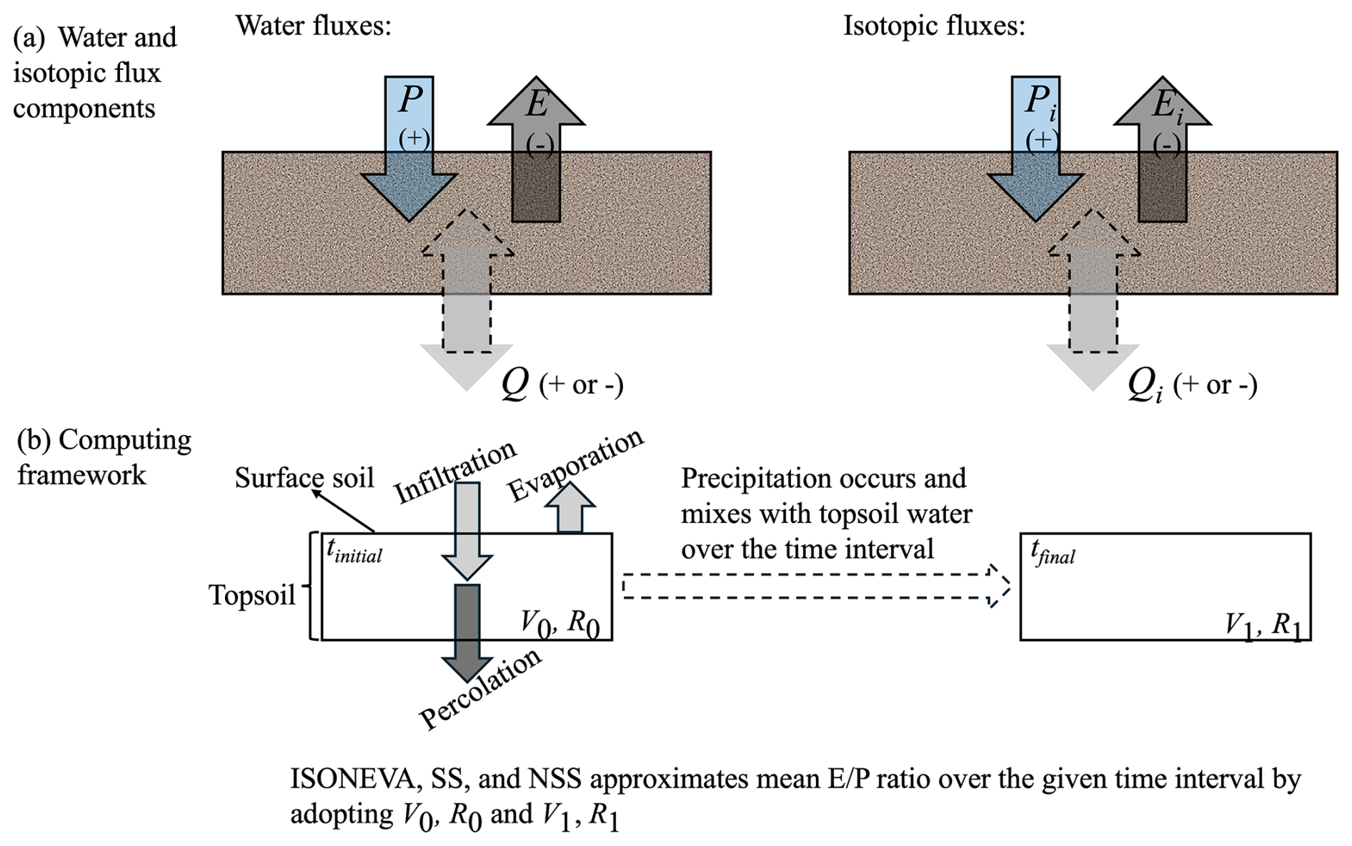
Figure 1 Conceptual illustration of the topsoil control volume and the water-isotope mass balance framework used in ISONEVA. (a) Schematic of water fluxes within the topsoil control volume, where P, E, and Q denote precipitation, evaporation, and percolation, respectively. Dashed arrows indicate that the direction of Q may reverse (upward or downward) depending on soil water potential gradients. (b) Conceptual diagram of the computational framework. ISONEVA, SS, and NSS use the initial (t_initial) and final (t_final) soil water content and isotopic composition (ratio, R) of the topsoil control volume to estimate the $E/P$ ratio over the specified evaluation period.

Based on the defined system, the soil water and isotope mass balance can be written as:

$$\begin{array}{}\text{(1)}& {\displaystyle \frac{\partial \mathit{\theta }}{\partial t}}=-{\displaystyle \frac{\partial q}{\partial z}}\text{(2)}& {\displaystyle \frac{\partial \left(\mathit{\theta }R\right)}{\partial t}}=-{\displaystyle \frac{\partial q_i}{\partial z}}\end{array}$$

Note that for the convenience of calculation, isotopic ratio (R) is used in this study, instead of notation δ. The conversion between R and δ is:

$$\begin{array}{}\text{(3)}& \mathit{\delta }={\displaystyle \frac{R-R_{\mathrm{ref}}}{R_{\mathrm{ref}}}}\mathrm{1000}\end{array}$$

where R_ref is the isotopic ratio reference value, 155.76 × 10⁻⁶ and 2005.2 × 10⁻⁶ for deuterium and oxygen-18, respectively.

Assuming the topsoil layer has a thickness of Δz and the variation of soil water and isotopic fluxes is uniform within the topsoil layer, then Eqs. (1) and (2) can be linearized as:

$$\begin{array}{}\text{(4)}& {\displaystyle \frac{\partial \mathit{\theta }}{\partial t}}=-{\displaystyle \frac{\left(Q-\left(P+E\right)\right)}{\mathrm{\Delta }z}}\text{(5)}& {\displaystyle \frac{\partial \left(\mathit{\theta }R\right)}{\partial t}}=-{\displaystyle \frac{\left(Q_i-\left(P_i+E_{\mathrm{i}}\right)\right)}{\mathrm{\Delta }z}}\end{array}$$

with relationships between water and isotopic fluxes are:

$$\begin{array}{}\text{(6)}& \left\{\begin{array}{l}{Q}_i=QR\\ P_i=P{R}_{\mathrm{P}}\\ E_{\mathrm{i}}=E{R}_{\mathrm{E}}\end{array}\right.\end{array}$$

where R, R_P, and R_E are isotopic ratio of soil water in the topsoil layer, precipitation, and evaporation, respectively. We define the isotopic composition of infiltration to be equal to that of precipitation (Fig. 1b). In addition, the isotopic composition of the outgoing percolation flux from the topsoil layer is assumed to be equal to the isotopic composition of the topsoil layer itself (Q_i= QR, Fig. 1b). This treatment follows the well-established well-mixed control-volume assumption, whereby the measured bulk isotopic composition of the topsoil layer represents the integrated mixing of incoming precipitation with pre-existing soil water and thus defines the isotopic composition of water leaving the control volume. This assumption is widely adopted in isotope hydrology and solute transport modelling in porous media (e.g., Ads et al., 2025; Braud et al., 2005; Haverd and Cuntz, 2010; Zhou et al., 2021), as well as in isotope-based evaporation studies of open-water bodies (e.g., Gonfiantini, 1986).

Defining the soil water storage (V) of the topsoil layer is θΔz, then Eqs. (4) and (5) can be rewritten as:

$$\begin{array}{}\text{(7)}& {\displaystyle \frac{\partial V}{\partial t}}=P+E-Q\text{(8)}& {\displaystyle \frac{\partial \left(VR\right)}{\partial t}}=P{R}_{\mathrm{P}}+E{R}_{\mathrm{E}}-QR\end{array}$$

Combining Eqs. (7) and (8), the $E/P$ ratio can be solved under different assumptions:

1. SS method: Steady state evaporation characterized with constant soil water volume and isotopic ratio.

   When soil evaporation reaches a steady state, temporal variations in soil water storage and isotopic composition within the uppermost soil layer become negligible ($\frac{\partial V}{\partial t}=$ 0 and $\frac{\partial \left(VR\right)}{\partial t}=$ 0). Under these conditions, Eqs. (7) and (8) can be rewritten as:

   $$\begin{array}{}\text{(9)}& {\displaystyle }P+E=Q\text{(10)}& {\displaystyle }P{R}_{\mathrm{P}}+E{R}_{\mathrm{E}}=QR\end{array}$$

   Defining the ratio of evaporation to precipitation ($E/P$) as x and the ratio of Q to P as y, both can be solved analytically from Eqs. (9) and (10):

   $$\begin{array}{}\text{(11)}& {\displaystyle }x={\displaystyle \frac{R-R_{\mathrm{P}}}{R_{\mathrm{E}}-R}}\text{(12)}& {\displaystyle }y={\displaystyle \frac{R_{\mathrm{E}}-R_{\mathrm{P}}}{R_{\mathrm{E}}-R}}\end{array}$$

   where R and R_P are measurable, R_E can be estimated using Craig-Gordon model:

   $$\begin{array}{}\text{(13)}& R_{\mathrm{E}}={\displaystyle \frac{E_{\mathrm{i}}}{E}}\end{array}$$

   where E and E_i are evaporative water and isotopic fluxes, respectively, based on the vapor concentration between soil surface and atmosphere:

   $$\begin{array}{}\text{(14)}& {\displaystyle }E={\displaystyle \frac{\mathrm{cvsat}{\mathrm{RH}}_{\mathrm{soil}}-\mathrm{cvsat}{\mathrm{RH}}_{\mathrm{atmos}}}{\mathit{\rho }}}\text{(15)}& {\displaystyle }{E}_{\mathrm{i}}={\displaystyle \frac{\mathrm{cvsat}{\mathrm{RH}}_{\mathrm{soil}}\mathit{\alpha }R-\mathrm{cvsat}{\mathrm{RH}}_{\mathrm{atmos}}{R}_{\mathrm{atmos}}}{{\mathit{\alpha }}_{\mathrm{k}}\mathit{\rho }}}\end{array}$$

   where cvsat is saturated vapor concentration, RH_soil and RH_atmos are soil and atmospheric relative humidity, respectively; R and R_atmos are isotopic ratio of soil and atmospheric water, α and α_k are equilibrium and kinetic fractionation factors (Fu et al., 2025). Note that the estimated value of x (Eq. 11) should be negative, as the negative sign indicates the direction of evaporation is opposite to that of precipitation (P).

   Consequently, Eq. (13) can be rewritten by combining Eqs. (13), (14), and (15):

   $$\begin{array}{}\text{(16)}& R_{\mathrm{E}}=AR-B\end{array}$$

   with $A=\frac{{\mathrm{RH}}_{\mathrm{soil}}\mathit{\alpha }}{{\mathit{\alpha }}_{\mathrm{k}}}$, $B=\frac{{\mathrm{RH}}_{\mathrm{atmos}}{R}_{\mathrm{atmos}}}{{\mathit{\alpha }}_{\mathrm{k}}}$.

2. NSS method: Non-steady state characterized by dynamic soil water volume and isotopic ratio, but caused by evaporation only.

   Under this framework, Eqs. (7) and (8) can be simplified as:

   $$\begin{array}{}\text{(17)}& {\displaystyle \frac{\partial V}{\partial t}}=E\text{(18)}& {\displaystyle \frac{\partial \left(VR\right)}{\partial t}}=E{R}_{\mathrm{E}}\end{array}$$

   Defining the ratio of final soil water storage (V) to the initial soil water storage (V₀) is f ($f=\frac{V}{V_{\mathrm{0}}}$). R can be analytically derived from Eqs. (17) and (18) (Derivations can be referred to Appendix A):

   $$\begin{array}{}\text{(19)}& R=-{\displaystyle \frac{B}{\mathrm{1}-A}}+f^{-\left(\mathrm{1}-A\right)}\left(R_{\mathrm{0}}+{\displaystyle \frac{B}{\mathrm{1}-A}}\right)\end{array}$$

   where R₀ is the initial soil water isotopic ratio; A and B are defined in Eq. (16). Note that Eq. (19) is generally written in the following form to estimate remaining water fraction of V₀ after evaporation:

   $$\begin{array}{}\text{(20)}& f={\left({\displaystyle \frac{R+\frac{B}{\mathrm{1}-A}}{R_{\mathrm{0}}+\frac{B}{\mathrm{1}-A}}}\right)}^{-\frac{\mathrm{1}}{\mathrm{1}-A}}\end{array}$$

   Then, the evaporative loss fraction of the initial soil water volume (f_e) can be calculated as:

   $$\begin{array}{}\text{(21)}& f_{\mathrm{e}}=\mathrm{1}-f=\mathrm{1}-{\left({\displaystyle \frac{R+\frac{B}{\mathrm{1}-A}}{R_{\mathrm{0}}+\frac{B}{\mathrm{1}-A}}}\right)}^{-\frac{\mathrm{1}}{\mathrm{1}-A}}\end{array}$$

   Consequently, the ratio of evaporation to precipitation, x, can be written as:

   $$\begin{array}{}\text{(22)}& x={\displaystyle \frac{V_{\mathrm{0}}{f}_{\mathrm{e}}}{P}}\end{array}$$

3. ISONEVA: Non-steady state evaporation characterized with dynamic soil water storage and isotopic ratio resulted from evaporative and non-evaporative fluxes.

   When evaporative and non-evaporative fluxes in the topsoil layer are considered, R can be derived from Eqs. (7) and (8) analytically (see Appendix A for derivations):

   $$\begin{array}{}\text{(23)}& R={\displaystyle \frac{R_{\mathrm{P}}-Bx}{\mathrm{1}-Ax+x}}+f^{-\frac{\mathrm{1}-Ax+x}{\mathrm{1}+x-y}}\left(R_{\mathrm{0}}-{\displaystyle \frac{R_{\mathrm{P}}-Bx}{\mathrm{1}-Ax+x}}\right)\end{array}$$

   Solutions of x and y from Eq. (23) are introduced in following sections and all parameters in Eq. (23) are already defined.

2.2 Method evaluation

2.2.1 Virtual test

The virtual test is adapted from a benchmark scenario describing isotope transport in an unsaturated soil column under non-isothermal conditions, which has been widely used for hydrological model validation studies (Fu et al., 2025; Zhou et al., 2021). To better reflect the complexity of land-atmosphere interactions, we designed two contrasting climatic regimes that generate distinct hydrological states and flux-partitioning behaviour: (i) an arid regime characterized by $|E/P|>\mathrm{1}$ (absolute ratio of E to P is greater than 1), and (ii) a humid regime characterized by $|E/P|<\mathrm{1}$ (absolute ratio of E to P is smaller than 1). For both regimes, MOIST outputs daily soil water and δ¹⁸O profiles as well as the evaporation and drainage (or non-evaporative) fluxes. These outputs are then used to evaluate SS, NSS, and ISONEVA by comparing their estimated $E/P$ ratios against the benchmark value of $E/P$ computed directly from MOIST-simulated fluxes. This virtual experiment serves as a controlled benchmark and it is designed to test our core hypothesis: by integrating both evaporative and non-evaporative fluxes, ISONEVA can estimate $E/P$ more accurately than existing methods.

2.2.2 Soil information

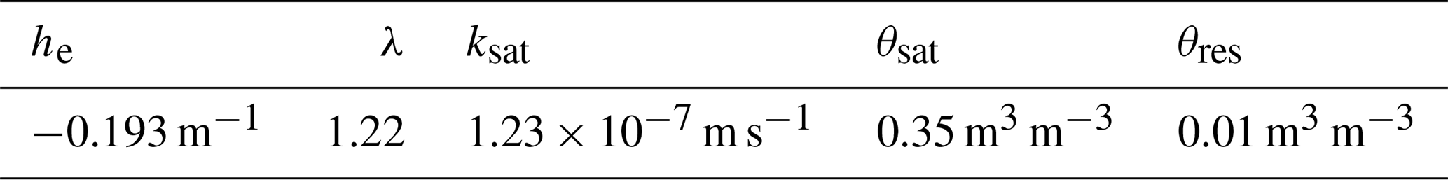
The simulated soil texture is Yolo light clay (Braud et al., 2005). The relationships between soil water content, pressure head, and unsaturated hydraulic conductivity for this soil type is described using the Brooks-Corey model (Brooks and Corey, 1964), with related parameters listed in Table 1.

Table 1 Soil hydraulic parameters of Yolo light clay used in forward simulation.

2.2.3 Initial and boundary conditions

The initial soil water content within this one-meter depth virtual column is uniformly distributed at 70 % saturated soil water content, while the initial isotope profile (δ¹⁸O) is uniformly distributed with a value of 0 ‰. The lower boundary is set to free drainage for both water and isotope transport, implying zero gradients in soil water potential and soil water isotopic composition at the bottom.

At the upper boundary, precipitation amount and the δ¹⁸O of rainfall are prescribed, while evaporation is controlled by potential evaporation (E_p) and atmospheric forcing. The isotopic composition of atmospheric vapor is set to δ¹⁸O = −14 ‰. Two climatic regimes are further defined to represent contrasting hydrological conditions:

1. Arid regime ($|E/P|>\mathrm{1}$). Air temperature (T_a) and relative humidity (RH_a) vary diurnally to mimic realistic non-steady atmospheric control on evaporation. T_a is prescribed as a sinusoidal cycle (daily maximum at mid-afternoon and minimum near sunrise: T_a= 30 + 10 ⋅ sin(2πt)), while RH_a varies inversely with T_a (RH_a= 0.5–0.3sin(2πt)). Potential evaporation E_p is set to 2 × 10⁻⁷ m s⁻¹. Rainfall occurs at low frequency (every 10 d, with each event lasting one day) with a flux of ϵ×3 × 10⁻⁷ m s⁻¹ per event, where ϵ is a random number between 0 and 1. This ensures total precipitation smaller than total evaporation, yielding $|E/P|>\mathrm{1}$ during the simulated period. The isotopic signature (δ¹⁸O) of each rainfall event is randomly assigned within the range −50 ‰ to −10 ‰ using −50 + ϵ × 40 (‰), which is sufficient to encompass the natural variability of precipitation δ¹⁸O observed across a wide range of climatic conditions (Nelson et al., 2021).

2. Humid regime ($|E/P|<\mathrm{1}$). Soil information is identical to that described in arid regime. T_a and RH_a follow the same diurnal structure as above, but E_p is reduced to represent weaker evaporative demand (5 × 10⁻⁸ m s⁻¹). Besides, rainfall occurs more frequently (every 2 d, with each event lasting one day) to increase the cumulative precipitation amount over the evaluation windows and yielding $|E/P|<\mathrm{1}$. Rainfall δ¹⁸O is also randomly assigned within the same climatologically plausible range to avoid regime-specific isotope tuning.

   These virtual scenarios cover two contrasting hydroclimatic regimes, isolating the effect of the hydrological state (arid vs. humid) on identifiability and model performance while keeping the soil type and numerical configuration consistent. The imposed atmospheric forcing and rainfall variability are chosen within climatologically realistic ranges, allowing the virtual experiment to capture essential features of real-world land-atmosphere interactions.

2.2.4 $E/P$ ratio evaluation

The forward simulation of these two scenarios is conducted by MOIST model under various spatial resolutions (Δz= 0.2, 0.1, and 0.05 m) within a one-meter depth column, whose capability to accurately simulate isotope transport in soil has been demonstrated previously (Fu et al., 2025). MOIST output daily soil water content and soil isotope profiles. Additionally, the benchmark $E/P$ ratio (and $Q/P$) can be calculated directly from the simulated evaporation (percolation) and precipitation fluxes provided by MOIST. These outputs from MOIST are used to evaluate backward calculation of $E/P$ from SS (Eq. 11), NSS (Eq. 19), and ISONEVA (Eq. 23) methods. Note that in the humid regime, precipitation events are prescribed every 2 d, resulting in a denser sequence of wetting-drying cycles than in the arid regime (every 10 d). Therefore, a shorter simulation period (50 d) is sufficient to generate a comparable (and larger) number of rainfall events and evaluation windows for method assessment, while keeping the numerical experiment computationally tractable. By contrast, the arid regime requires a longer simulation (100 d) to include an adequate number of rainfall events and to span multiple multi-day aggregation windows under infrequent forcing. Consequently, the two regimes are configured with different simulation lengths to ensure comparable information content (event count and window samples) rather than identical duration.

To ensure consistency with typical field sampling practice, we evaluate multiple temporal windows (every 5 d in the humid regime and every 2 d in the arid regime) and three representative topsoil thicknesses (Δz= 0.05, 0.10, and 0.20 m), reflecting common sampling depths and frequencies (Dubbert et al., 2013; Shokri et al., 2008). Each temporal window is defined such that at least one rainfall event occurs within the interval. For a given temporal window, the initial and final soil water content and isotopic composition of the defined topsoil layer are extracted from MOIST outputs and used to estimate $E/P$ over that period. For example, in a 5 d window, soil water content and isotopic composition on Day 1 and Day 5 are used to estimate the cumulative $E/P$ for those five days. This procedure is repeated across all spatial resolutions to assess the sensitivity of SS, NSS, and ISONEVA to topsoil thickness and temporal aggregation.

Note that δ²H and δ¹⁸O in soil water can be strongly linearly correlated, resulting in near collinearity in isotope space. Consequently, they provide largely redundant rather than independent constraints on the unknown flux ratios and cannot be jointly used to uniquely constrain both x and y. In addition, δ¹⁸O generally exhibits smaller analytical uncertainty compared to δ²H, which reduces noise propagation during the inversion and improves numerical stability. Therefore, δ¹⁸O is selected as the representative tracer in this study.

Since SS and NSS contain only one unknown, which can be solved directly using output data from MOIST. By contrast, ISONEVA originally involves two unknowns, x= $E/P$ and y= $Q/P$, but only one isotope-based equation, which makes the problem underdetermined if treated purely as a two-unknown inversion. To improve identifiability and enforce mass conservation more rigorously, we derived a water-balance constraint from the observed change in topsoil water storage over the evaluation window (Eq. 7):

$$\begin{array}{}\text{(24)}& {\displaystyle \frac{\mathrm{\Delta }V}{P}}=\mathrm{1}+x-y\end{array}$$

where ΔV is the change in water storage of the topsoil layer and P is cumulative precipitation over the same interval. This constraint allows y to be eliminated in Eq. (23) and reduces the inversion to a one-dimensional optimization problem in x. By explicitly enforcing mass conservation, this reformulation removes the structural non-uniqueness associated with unconstrained (x, y) search.

Despite dimensionality reduction, the objective function remains highly nonlinear in x (Eq. 23) due to its ratio structure and exponential dependence, which may cause numerical instability under certain hydrological states. As a result, the objective function (Eq. 23) may exhibit strong curvature or local flat regions under certain hydrological states, potentially affecting numerical convergence and solution stability. We adopt the following optimization strategy to solve x:

• Single-window inversion (default). For each evaluation window, x is estimated by minimizing the isotope residual objective with y analytically eliminated using the storage constraint (Eq. 24). The optimization is performed using a bounded one-dimensional search (fminbnd function in MATLAB), which ensures deterministic and reproducible solutions within physically meaningful limits.

• Multi-window coupled inversion (fallback). When a single evaluation window provides insufficient information content (e.g., weak storage change, near-steady-state conditions, boundary convergence, or numerical degeneracy), we implement a multi-window coupled inversion strategy. In this approach, x is assumed to remain constant within a short predefined block (up to three consecutive windows), and isotope mass balance constraints from these windows are jointly used to estimate a single value of x. For instance, if the inversion over an initial 5 d window does not yield a stable interior solution, subsequent consecutive windows (e.g., Days 1–10 and/or Days 1–15) are incorporated, and a common x is estimated using the combined constraints. By aggregating multiple end-point isotope and storage-change signals, this strategy increases the effective information content while maintaining a physically interpretable assumption of quasi-constant flux partitioning over short time scales.

  Although assuming constant x within a block may introduce limited approximation error if flux partitioning varies temporally, it represents a controlled bias-variance trade-off that substantially enhances parameter identifiability under weak-signal conditions and prevents spurious boundary-constrained solutions. In practice, the block length is deliberately restricted to a maximum of three windows to minimize potential bias while improving numerical stability.

To quantify uncertainty and avoid reliance on stochastic optimizer variability, measurement uncertainties are propagated through the inversion using Monte Carlo simulation. Specifically, we perturb (i) topsoil δ¹⁸O measurements and (ii) precipitation δ¹⁸O data by adding Gaussian noise (measurement error) with a standard deviation of 0.7 ‰ (von Freyberg et al., 2020), recompute x for each perturbed realization (1000 simulations per window), and report uncertainty as the standard deviation of the resulting x. This approach explicitly links reported uncertainty to observational error, thereby providing a physically interpretable confidence estimate.

2.2.5 Field test

Site description

The field experiment is conducted on continuously weighted soil lysimeters, situated at the École Polytechnique Fédérale de Lausanne (EPFL), in Switzerland (Nehemy et al., 2021). Lysimeters are exposed to atmospheric conditions and monitored for a period of 43 d after the application of an isotopically labelled irrigation event on the 16 May 2018, ending on the 29 June 2018. One bare lysimeter and one vegetated lysimeter are used to monitor evaporation and evapotranspiration, respectively.

Measured data

Within the vegetated lysimeter, soil water content is measured at four depths (0.25, 0.75, 1.25, and 1.75 m) using frequency domain reflectometry probes (FDR; 5TM Devices Inc., USA), while soil water isotopic compositions are sampled at five depths (0.1, 0.25, 0.5, 0.8, and 1.5 m) with two replications at each depth (Fig. 2e) and analyzed at the Watershed Hydrology Lab at the University of Saskatchewan. To harmonize the spatial scales of these two datasets, we define 0–0.25 m as the topsoil layer. Details about the experiment and sample processing can be referred to Nehemy et al. (2021).

Since evaporation measurements from the neighbour bare lysimeter are only available between 4 and 29 June, thus, the field validation in this study is conducted over this period. Within this period, the daily evaporation rate (measured by the bare soil lysimeter) ranged from 0.97 to 2.27 mm d⁻¹ (Fig. 2a). Three precipitation events (including artificial irrigation) took place on 10, 14 and 26 June. The smallest daily input is 69.2 mm d⁻¹ (on 10 June), while the largest input is 193.5 mm d⁻¹ (on 26 June) (Fig. 2b). The input isotopic signals showed a gradual depletion as the precipitation amount increased (Fig. 2c). Under this water input pattern, soil water content in the topsoil layer (0–0.25 m) shows a “rise-decline-rise” trend (Fig. 2d).

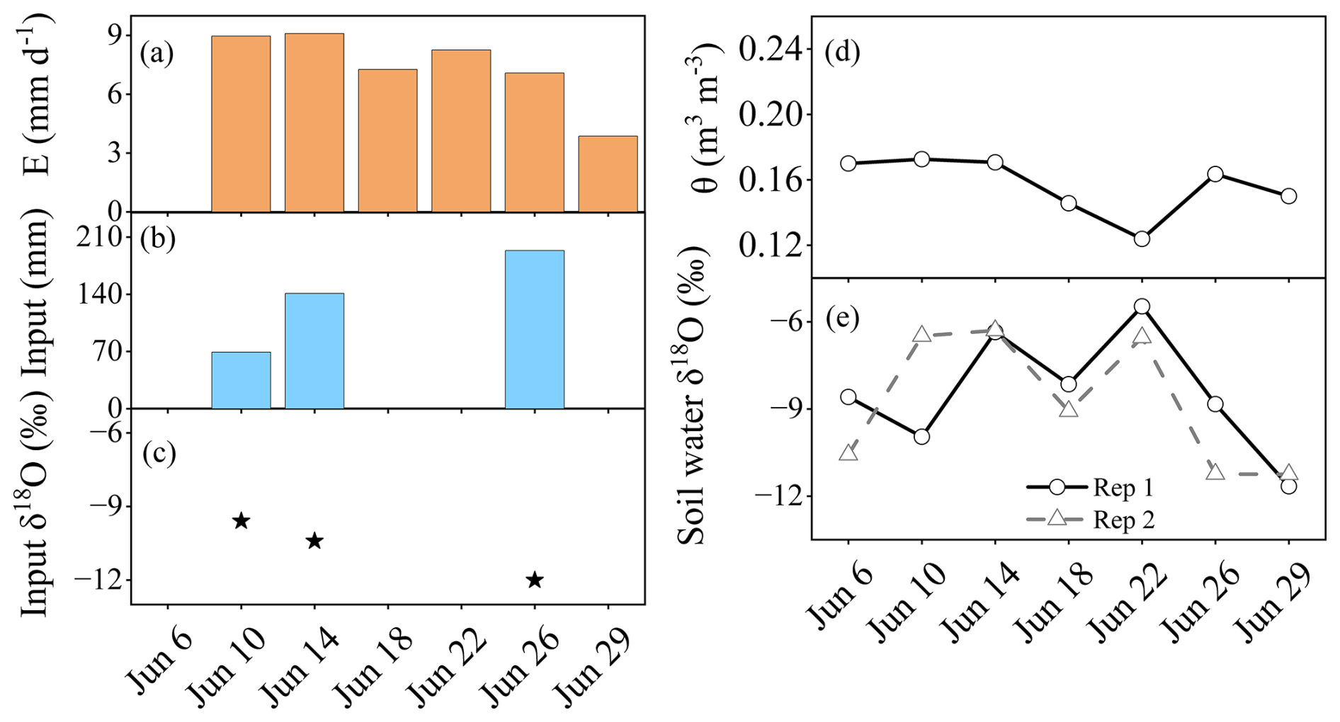
Figure 2 Measured evaporation (a), input water (precipitation + irrigation, b) and isotope signals (c), soil water contents (d) and isotopic signals with two replications (e) from 6 to 29 June. Note that 6 June is the initial date.

$E/P$ estimation

Following the sampling frequency from Nehemy et al. (2021), several time intervals (4, 8, 12, 16, 20, and 24 d) are defined to estimate the $E/P$ ratio for each period, starting from 4 June. Meanwhile, actual $E/P$ ratios are calculated using evaporation data from the bare lysimeter, serving as a benchmark for evaluating the performance of SS, NSS, and ISONEVA.

The potential daily evaporation (E_p) is conservatively assumed to range between 0 and 10 mm d⁻¹, covering the plausible variability observed during the experimental period. Accordingly, the physically admissible bounds of $E/P$ are constrained by the ratio between cumulative potential evaporation and cumulative precipitation within each evaluation interval, ensuring that the search space remains consistent with realistic hydrological limits.

Under the imposed mass conservation constraint (Eq. 24), the non-evaporative flux ratio $Q/P$ (y) is analytically determined from the estimated x and the observed storage change, rather than independently optimized. This formulation guarantees internal consistency between water balance and isotope-based inversion.

Uncertainty in x is quantified by propagating isotopic measurement uncertainty through Monte Carlo simulation. Specifically, repeated isotope measurements are used to estimate the empirical standard deviation of δ¹⁸O. Gaussian perturbations based on this standard deviation are applied to the isotope observations, and the inversion is recomputed for each realization. The resulting distribution of $E/P$ estimates (1000 realizations per interval) is summarized as mean ± standard deviation.

The isotopic composition of infiltration is set equal to that of rainfall, which is a standard measurement during field campaigns and has been justified in Fig. 1. For the non-evaporative flux, we assign the isotopic composition of the topsoil water. This is justified because (1) non-evaporative flux is expected to cause insignificant isotopic fractionation, and (2) the isotopic composition of topsoil water is directly measurable. Additionally, due to the absence of in situ measurements of isotopic compositions in atmospheric vapor, we adopt reference values of δ¹⁸O = −20 ‰ based on cold-trap measurements conducted in Vienna under comparable climatic and seasonal conditions (Kurita et al., 2012). Global water vapor isotope studies indicate that central European stations exhibit strong spatial coherence in vapor isotopic composition, with δ¹⁸O values typically clustering between −25 ‰ and −15 ‰ because of the dominant mid-latitude westerly circulation (Galewsky et al., 2016). Because the EPFL site in Lausanne is located within this same large-scale meteorological regime, its atmospheric δ¹⁸O is expected to fall within this characteristic range.

To account for uncertainty in atmospheric vapor isotopic composition, the inversion was repeated using three plausible δ¹⁸O values (−25 ‰, −20 ‰, and −15 ‰). Measurement uncertainty of isotopic compositions in soil water is further propagated through repeated sampling during the inversion procedure. The resulting flux estimates are reported as mean ± SD, which jointly reflect uncertainties arising from both atmospheric vapor isotopic composition and isotope measurement error.

ET partition

In the ISONEVA framework, Q represents the total non-evaporative flux within the topsoil control volume and may include contributions from root water uptake, percolation, or other subsurface exchanges. The ratio derived from the ISONEVA framework is $\frac{\left|\frac{E}{P}\right|}{\left|\frac{E}{P}\right|+\left|\frac{Q}{P}\right|}=\frac{\left|E\right|}{\left|E\right|+\left|Q\right|}$, while the true ratio of E to ET is $\frac{\left|E\right|}{\left|E\right|+T_{\mathrm{total}}}$. The relationship between these two quantities depends on the relative magnitude of Q and T_total, where T_total is the total transpiration within the estimating time window.

Within the time interval that ISONEVA is applied, if the non-evaporative flux within the topsoil does not exceed T_total (Q ≤ T_total), then $\frac{\left|E\right|}{\left|E\right|+\left|Q\right|}\ge \frac{\left|E\right|}{\left|E\right|+T_{\mathrm{total}}}$ and $\frac{\left|E\right|}{\left|E\right|+\left|Q\right|}$ from ISONEVA represents an upper bound of the true $E/\mathrm{ET}$. By contrast, if additional subsurface fluxes within the topsoil become substantial (e.g., strong percolation or lateral flow), it is possible for Q to exceed total transpiration (|Q|>T_total). Then, the ratio $\frac{\left|E\right|}{\left|E\right|+\left|Q\right|}$ would underestimate the true value.

However, in the lysimeter validation used in this study, hydrometric observations (Benettin et al., 2021) provide evidence that the non-evaporative flux within the topsoil control volume is likely smaller than total plant transpiration during the experimental period. The lysimeter experiment is characterized by high evapotranspiration rates (5–20 mm d⁻¹) and mostly negligible bottom drainage. Tracer-based water balance analysis further showed that transpiration accounted for approximately 58 % of the exported water, whereas bottom drainage contributed only about 10.4 %. In addition, soil water observations from the lysimeter (Nehemy et al., 2021) indicate that no sustained downward drainage occurred during the experimental period. Together, these observations suggest that the non-evaporative flux is therefore likely smaller than total transpiration from the entire rooting zone (|Q| ≤ T_total). Consequently, the ratio derived from ISONEVA, $\frac{\left|E\right|}{\left|E\right|+\left|Q\right|}$, represents a conservative upper bound of the true evaporation fraction $\frac{E}{\mathrm{ET}}$.

2.2.6 Method accuracy

In both the virtual and field validations, SS and NSS are applied using the same inputs, temporal resolution, and initial and final soil water and isotope profiles as the ISONEVA method. This ensures a fair comparison, removing the potential effects of data on the performance improvement of ISONEVA.

Accordingly, to quantify the accuracy of the average $E/P$ value approximated by SS, NSS, and ISONEVA, we assess model performance using the mean absolute error (MAE):

$$\begin{array}{}\text{(25)}& \mathrm{MAE}={\displaystyle \frac{{\sum }_{i=\mathrm{1}}^N\mathrm{abs}\left({\mathrm{EP}}_{\mathrm{ei}}-{\mathrm{EP}}_{\mathrm{mi}}\right)}{N}}\end{array}$$

where EP_ei and EP_mi are estimated and measured (or estimated from MOIST in virtual tests) $E/P$ values; N is the total number of measurements; i is the ith measurement.

3 Results

3.1 Comparison of estimated $E/P$ and $Q/P$ ratios between SS, NSS, and ISONEVA from virtual dataset

3.1.1 Arid regime ($|E/P|>\mathrm{1}$)

The benchmark $E/P$ values derived from MOIST simulations (black circles in Fig. 3) are consistently smaller than −1, indicating an evaporation-dominated water balance throughout the simulation period (arid regime). For $E/P$ backward estimation, both SS and NSS show substantial deviations from the simulated values, with MAE values of 2.07, 1.73, and 1.38 for SS and 2.49, 2.08, and 1.76 for NSS under Δz= 0.2, 0.1, and 0.05 m, respectively (Fig. 3a–c). These discrepancies arise from the structural assumptions of the two approaches. The SS formulation assumes negligible changes in topsoil water storage, while NSS accounts for storage dynamics but neglects non-evaporative fluxes such as infiltration and percolation. Both assumptions are inconsistent with the simulated conditions, where topsoil water balance is simultaneously influenced by evaporation, precipitation, and vertical water exchange.

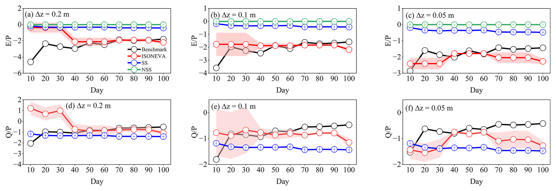
Figure 3 Performance of SS, NSS, and ISONEVA in estimating $E/P$ and $Q/P$ ratios under the arid regime ($|E/P|>\mathrm{1}$). Panels (a)–(c) show the estimated $E/P$ ratios for three topsoil thicknesses (Δz= 0.2, 0.1, and 0.05 m), while panels (d)–(f) show the corresponding $Q/P$ ratios. Black circles represent the benchmark values derived from MOIST simulations, blue circles represent the SS method, green circles represent the NSS method, and red circles represent the ISONEVA estimates. Shaded areas indicate the uncertainty ranges derived from Monte Carlo simulations accounting for δ¹⁸O measurement uncertainty (±0.7 ‰).

By contrast, ISONEVA produces $E/P$ estimates that closely follow the simulated values across most time windows and spatial resolutions. Although noticeable deviations and relatively large uncertainty ranges occur during the earliest evaluation periods, the estimates rapidly converge toward the benchmark values as the temporal window increases (Fig. 3a–c). Compared with SS and NSS, the estimation accuracy of ISONEVA improves by 49.8 %–58.3 %, 74.7 %–79.0 %, and 65.4 %–72.9 % under Δz= 0.2, 0.1, and 0.05 m, respectively. This improved performance arises because ISONEVA explicitly resolves both evaporative and non-evaporative fluxes while simultaneously enforcing dynamic water storage constraints in the topsoil layer.

For $Q/P$ estimation (Fig. 3d–f), NSS cannot provide estimates because non-evaporative fluxes are not included in its formulation. Under arid conditions, the simulated $Q/P$ values are negative, indicating an upward compensating flux from deeper soil layers. SS provides relatively better approximations of $Q/P$ than $E/P$. This behaviour likely results from error compensation associated with the steady-state assumption, where biases in $E/P$ estimation partially propagate into the derived $Q/P$ ratio. Nevertheless, ISONEVA still improves the accuracy of $Q/P$ estimation compared with SS, with MAE reductions of 24.2 %, 30.7 %, and 65.0 % under Δz= 0.2, 0.1, and 0.05 m, respectively.

Uncertainty in ISONEVA estimates of $E/P$ and $Q/P$ ratios is relatively large during early evaluation windows but decreases as the temporal window expands. By contrast, SS and NSS show much narrower uncertainty ranges (Fig. 3). Although identical Monte Carlo perturbations (±0.7 ‰ for δ¹⁸O in soil water) are applied to all methods, the SS and NSS formulations rely on closed-form ratio expressions in which isotope values appear in both the numerator and denominator. As a result, small perturbations in isotope measurements tend to partially cancel, leading to limited propagation of measurement uncertainty. By contrast, ISONEVA estimates flux ratios through a nonlinear inversion that combines isotope mass balance with dynamic soil water storage constraints. Under short evaluation windows, changes in soil water storage and isotope composition are small, resulting in limited information content for constraining the inversion. In this situation, ISONEVA can result in large uncertainties from small soil water isotopic perturbations. As the temporal window increases, the inversion becomes progressively better constrained, and the associated uncertainty correspondingly decreases.

3.1.2 Humid regime ($|E/P|<\mathrm{1}$)

Under humid conditions, the benchmark $E/P$ values derived from the MOIST simulations (black circles, Fig. 4) remain between −1 and 0 throughout the simulation period, indicating a precipitation-dominated hydrological regime. Compared with the arid regime, SS produces relatively reasonable $E/P$ estimates, with MAE values of 0.41, 0.42, and 0.33 under Δz= 0.2, 0.1, and 0.05 m, respectively. Nevertheless, these errors remain larger than those obtained from ISONEVA (0.24, 0.15, and 0.10). Additionally, NSS continues to exhibit the largest deviations (MAE = 0.86, 0.84, and 0.78) in $E/P$ estimates across all spatial resolutions.

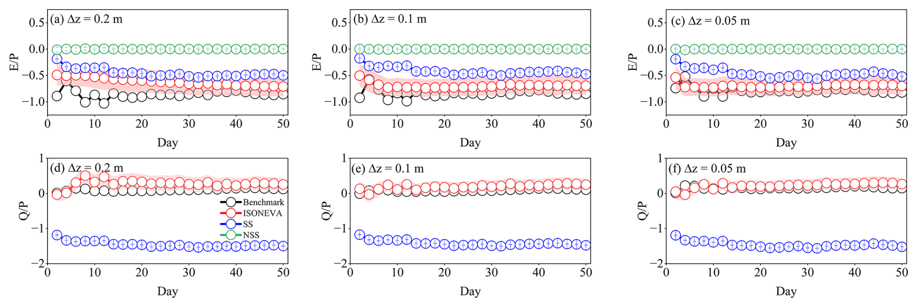
Figure 4 Comparison of estimated $E/P$ and $Q/P$ ratios from SS, NSS, and ISONEVA under the humid regime ($|E/P|<\mathrm{1}$) using the virtual dataset generated by the MOIST model. Panels (a)–(c) show the estimated $E/P$ ratios, while panels (d)–(f) present the corresponding $Q/P$ ratios. The black circles represent the benchmark values derived directly from the simulated evaporation, precipitation, and percolation fluxes. Red circles denote estimates from ISONEVA, blue circles from SS, and green circles from NSS. Results are shown for three topsoil thicknesses (Δz= 0.2, 0.1, and 0.05 m). The shaded regions indicate the uncertainty ranges derived from Monte Carlo simulations accounting for δ¹⁸O measurement uncertainty (±0.7 ‰).

The performance patterns differ for $Q/P$ estimation. Under humid conditions, SS shows substantial bias in estimating $Q/P$ with MAE values are 1.55 (Δz= 0.2 m), 1.50 (Δz= 0.1 m), 1.61 (Δz= 0.05 m), whereas ISONEVA continues to reproduce the simulated $Q/P$ values with higher accuracy (Fig. 4d–f) and respective MAE are 0.18, 0.11, 0.09. This discrepancy arises because the SS formulation neglects temporal changes in soil water storage and therefore cannot correctly partition precipitation inputs between evaporation and non-evaporative fluxes. Under humid conditions, frequent precipitation events induce substantial changes in soil water storage, violating the steady-state assumption underlying SS. By contrast, ISONEVA provides more physically consistent estimates of $Q/P$ by explicitly accounting for both storage dynamics and non-evaporative fluxes.

3.1.3 Sensitivity analysis

Sensitivity of ISONEVA to regime and topsoil thickness

To synthesize the sensitivity of the inversion performance to hydrological regime and sampling configuration, Table 2 summarizes the mean absolute error (MAE) and the mean standard deviation (SD) of $E/P$ estimates from ISONEVA under different topsoil thicknesses and associated multi-window settings.

Table 2 ISONEVA inversion performance to hydrological regime and topsoil thickness. Mean absolute error (MAE) of estimated $E/P$ ratios is reported for different sampling depths under arid and humid regimes. The “multi-window number” denotes the number of expanding windows used in the inversion to obtain a stable solution when single-window information is insufficient.

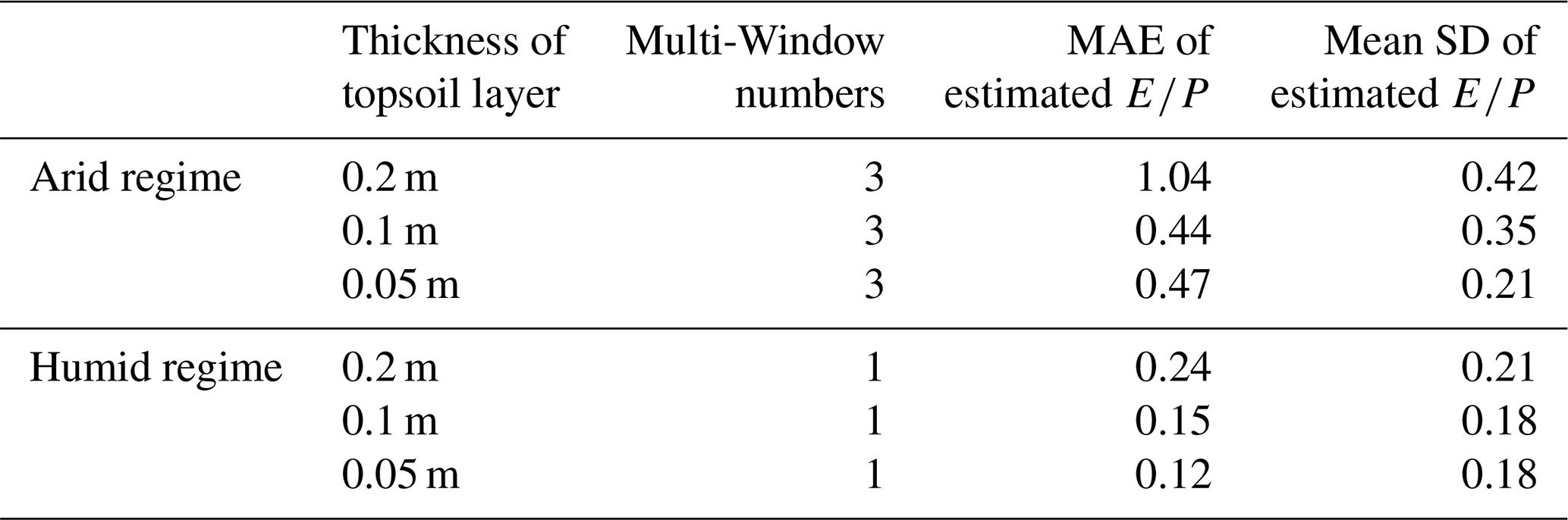
Under arid conditions, estimation errors of $E/P$ remain relatively large across all sampling depths, with MAE values of 1.04, 0.44, and 0.47 for Δz= 0.2, 0.1, and 0.05 m, respectively. In this regime, the inversion frequently relies on the multi-window strategy (up to three expanding windows) to obtain stable solutions. This behavior reflects the limited information content of individual evaluation windows under arid conditions. Because rainfall events occur infrequently, it introduces weak perturbations to topsoil water storage and isotopic composition within each window. Consequently, the isotope signal from a single window often provides insufficient constraints for resolving $E/P$, requiring the use of multiple expanding windows and resulting in larger estimation errors. Consistent with this pattern, the mean uncertainty is also higher under arid conditions, with SD values ranging from 0.21 to 0.42.

By contrast, under humid conditions the inversion becomes substantially more stable. The MAE values decrease to 0.24, 0.15, and 0.12 for Δz= 0.2, 0.1, and 0.05 m, respectively, and the optimal solutions are typically obtained using a single window. This improvement reflects the stronger storage signals and more frequent precipitation inputs in humid regimes, which increase the information content available for ISONEVA to estimate $E/P$. Correspondingly, the associated uncertainties are smaller and remain relatively consistent across sampling depths (SD ≈ 0.18–0.21). As a result, ISONEVA achieves higher accuracy and stability under humid than arid conditions.

Sampling depth also influences estimation performance of ISONEVA. Under arid conditions, MAE decreases markedly by about 58 % when the topsoil thickness is reduced from 0.2 to 0.1 m (from 1.04 to 0.44), whereas slightly increased 7 % from 0.1 to 0.05 m. A similar pattern is observed under humid conditions, where MAE decreases by about 38 % from 0.2 to 0.1 m (0.24 to 0.15), but 20 % from 0.1 to 0.05 m (0.15 to 0.12). This pattern reflects a trade-off between signal smoothing and measurement sensitivity. Thicker topsoil (0.2 m) tends to smooth isotope signals and reduce sensitivity to short-term flux dynamics, whereas thinner topsoil (0.05 m) may amplify short-term variability and become more sensitive to measurement noise. Overall, these results demonstrate that the identifiability of $E/P$ using ISONEVA is strongly controlled by the information content of isotope and storage signals, which in turn depends on hydrological regime and topsoil thickness.

Sensitivity of ISONEVA to atmospheric isotopic composition

To evaluate the sensitivity of ISONEVA to the atmospheric isotopic composition, we repeated the inversion using four prescribed values of atmospheric δ¹⁸O (−10 ‰, −14 ‰, −20 ‰, and −30 ‰), where −14 ‰ corresponds to the value used in the MOIST simulations (also corresponds to the results reported in Figs. 3 and 4). The resulting MAE values of $E/P$ estimates under different hydrological regimes and sampling depths are summarized in Table 3.

Table 3 Sensitivity of ISONEVA performance to the prescribed atmospheric δ¹⁸O. Mean absolute error (MAE) of $E/P$ estimates under arid and humid regimes is shown for different topsoil thicknesses. The reference atmospheric isotope composition (−14 ‰) corresponds to the value used in forward and backward simulations in this study, while −10 ‰ , −20 ‰, and −30 ‰ represent alternative plausible atmospheric vapor isotope conditions used to evaluate ISONEVA sensitivity.

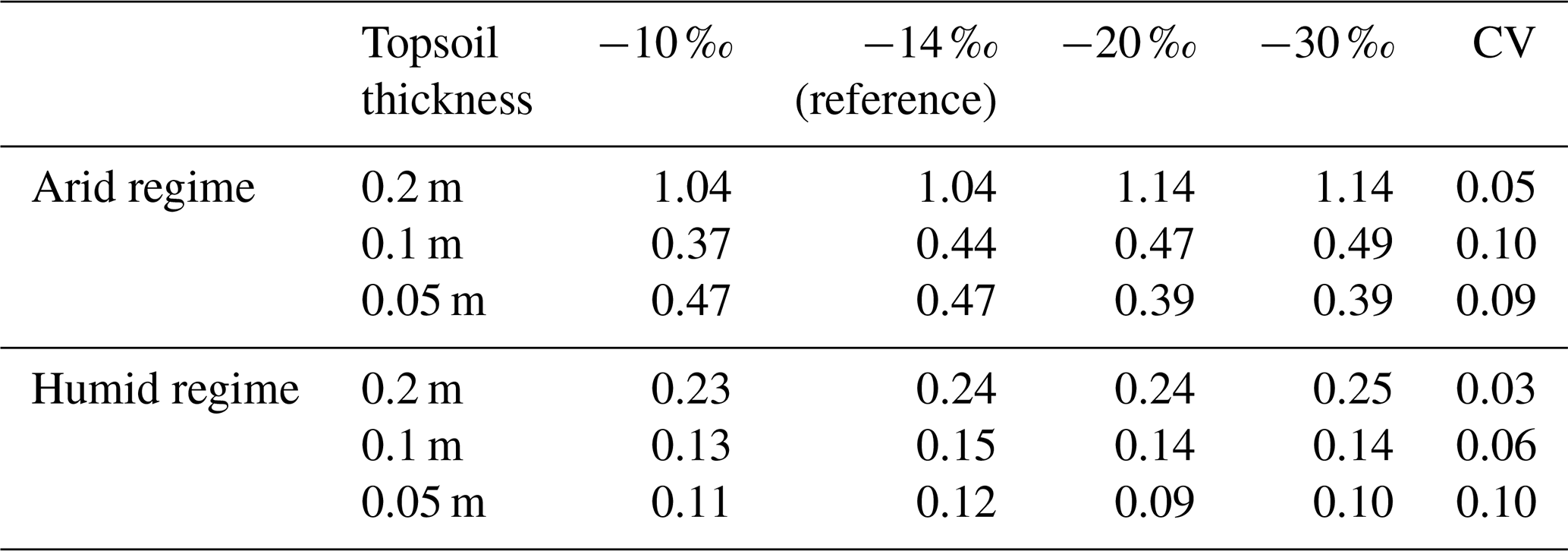
The performance of ISONEVA shows limited sensitivity to the prescribed atmospheric δ¹⁸O values. Across the tested range (−10 ‰ to −30 ‰), MAE values vary only moderately. Under arid conditions, MAE differences across atmospheric δ¹⁸O scenarios remain within approximately 0.08–0.12, depending on sampling depth. The coefficient of variation (CV) of MAE further indicates that the sensitivity of ISONEVA to atmospheric δ¹⁸O decreases with increasing topsoil thickness, with thicker topsoil layers exhibiting smaller CV values (Table 3).

A similar but even weaker sensitivity is observed under humid conditions. In this regime, the variation of MAE across atmospheric δ¹⁸O scenarios is considerably smaller, typically within 0.01–0.02 (Table 3). The corresponding CV values also show a decreasing trend with increasing topsoil thickness, indicating that $E/P$ estimates from thicker topsoil is less sensitive to atmospheric isotopic compositions than the thinner one.

Overall, the relationship between model performance and topsoil thickness is not strictly monotonic. As shown in Tables 2 and 3, thicker topsoil layers tend to smooth short-term isotope fluctuations and reduce sensitivity to uncertainties in atmospheric δ¹⁸O, but excessive thickness (e.g., 0.2 m) can dilute isotope signals and lead to larger estimation errors (especially under the arid regime). Conversely, very thin topsoil (e.g., 0.05 m) preserves stronger isotope signals and can improve estimation accuracy, but it also becomes more sensitive to external parameters such as atmospheric isotope composition (especially under the humid regime). As a result, this trade-off also interacts with the hydrological regime, as precipitation frequency and storage dynamics influence the information content available for constraining the inversion. A topsoil of 0.1 m would provide the balance between estimation accuracy and sensitivity.

3.2 Field test

Field validation of the SS, NSS, and ISONEVA methods over a 23 d period (6–29 June) is shown in Fig. 5, based on soil water and isotopic measurements from a vegetated lysimeter experiment under real-world conditions.

Figure 5 Estimated and measured $E/P$ ratios from lysimeter data under different temporal intervals. The shaded pink area represents the uncertainty of ISONEVA estimates. The date is shown on the lower x axis.

Among these three methods, SS produced moderate agreement with the measured $E/P$ values (MAE = 0.07), but the estimates showed noticeable variability across time intervals and occasionally deviated from the observations. However, the NSS method, which relaxes the steady soil water storage assumption, showed only limited improvement (MAE = 0.12) and still systematically underestimated $E/P$. This bias arises because NSS neglects non-evaporative fluxes (e.g., infiltration) that influence the soil water balance in field conditions.

By contrast, the ISONEVA method delivered the highest accuracy (MAE = 0.03), closely aligning with the measured $E/P$ values throughout the observation period. In addition, the uncertainty of ISONEVA estimates decreases progressively as the evaluation window expands, indicating that longer temporal integration provides stronger constraints for the inversion. This pattern is consistent with the humid-regime behaviour observed in the virtual experiments and further highlights the importance of explicitly accounting for both evaporative and non-evaporative fluxes when estimating soil evaporation using field-measured isotope data.

Additionally, cumulative ET from the vegetated lysimeter was 351.25 mm, and cumulative E from the bare lysimeter was 44.25 mm, yielding an observed $E/\mathrm{ET}$ ratio of 0.126. Based on the total precipitation input (403.65 mm) and the absolute $E/P$ ratio estimated by ISONEVA over this 23 d period (0.11 ± 0.04), the inferred $E/\mathrm{ET}$ ratio is 0.126 ± 0.04, which agrees well to the observed ratio. By comparison, the SS and NSS methods yielded significantly lower $E/\mathrm{ET}$ values of 0.02 and 0.01, respectively, substantially underestimating soil water evaporation.

Moreover, the $Q/P$ ratios from ISONEVA and SS are 0.90 ± 0.04 and 1.01 ± 0.01, respectively. Even in the absence of direct ET measurements, ISONEVA provides a maximum conservative upper bound estimate of $E/\mathrm{ET}$ as 0.15, which successfully encompassed the observed value (0.13). By contrast, the upper bound from SS is 0.02 and NSS failed to do so. This further demonstrates the practical utility of ISONEVA in real-world applications.

4 Discussion

4.1 ISONEVA improves solution space and avoids potential issues from identifying initial values

ISONEVA provides more accurate estimates than the SS and NSS methods because it explicitly integrates temporal changes in soil water storage and isotopic composition together with both evaporative and non-evaporative fluxes. By contrast, the SS and NSS methods ignore temporal changes in soil water storage and isotopic composition or non-evaporative fluxes and therefore do not enforce the water-balance constraint. As a result, their estimates of $E/P$ and $Q/P$ can vary substantially under different precipitation regimes. For example, Figs. 3 and 4 show that $E/P$ estimates from SS can approach the benchmark values under humid conditions but produce strongly biased $Q/P$ estimates, whereas under arid conditions the opposite pattern emerges. This contrasting behaviour indicates that apparent agreement with the benchmark values does not necessarily reflect a correct representation of the underlying processes. Because SS assumes steady soil water storage, any mismatch among precipitation, evaporation, and storage change must be implicitly compensated by the estimated flux ratios. As precipitation regimes change, the direction and magnitude of this compensation also change, which explains why SS may appear accurate under certain conditions but fail under others. Consequently, when SS produces closer estimates of $E/P$, the derived $Q/P$ can become biased, and vice versa. This mechanism is further supported by the field experiment, where SS produced $Q/P$ estimates over the experimental period greater than 1, which is physically implausible for the studied system. By contrast, ISONEVA simultaneously constrains both $E/P$ and $Q/P$ by explicitly accounting for dynamic soil water storage and non-evaporative fluxes, allowing the method to generate more consistent flux estimates across different hydrological regimes.

Moreover, ISONEVA avoids the common pitfalls associated with defining initial isotopic values associated with NSS. Many studies determine the initial isotopic composition using the intersection of the evaporation line (EL) with the local meteoric water line (LMWL) when using NSS framework (Benettin et al., 2021; Sprenger et al., 2017), implicitly assuming isotopic homogeneity and purely evaporative processes (Javaux et al., 2016). Heterogeneous mixing, new precipitation inputs, and vapor diffusion often disrupt these assumptions in soils. Importantly, the intersection-derived value does not necessarily represent the actual isotopic composition of the initial soil water storage (Benettin et al., 2018). Consequently, the EL-LMWL intersection often fails to reflect the true evaporation trajectory, potentially resulting in large initial value errors, up to −50 ‰ for δ²H and −8 ‰ for δ¹⁸O (Benettin et al., 2018). These errors can propagate through evaporation estimates, highlighting a critical limitation of NSS in natural, thus intrinsically heterogeneous, soil systems.

Additionally, the so-called “initial value” refers to the isotopic composition of water in the topsoil layer at a specific point in the solution of the governing partial differential equation (Gonfiantini, 1986). This “initial value” is relative rather than absolute: It does not necessarily correspond to the original isotopic compositions at the physical onset of evaporation. Instead, it marks the beginning of a defined calculation period.

ISONEVA circumvents this issue by redefining the initial value as a relative, temporally resolved parameter corresponding to the specific analysis period rather than an absolute physical starting point. This flexible treatment allows continuous, period-specific evaporation estimates without relying on potentially biased EL-LMWL intersections. Despite the increased computational complexity, ISONEVA offers a more physically reliable framework for estimating soil evaporation. With advances in in-situ soil isotope monitoring (Beyer et al., 2020; Volkmann and Weiler, 2022), ISONEVA can be coupled with isotope-enabled land surface models to evaluate soil-water and isotope trajectories for evaluating model performance or to directly constrain model-estimated $E/P$ ratios.

4.2 Practical considerations of ISONEVA for field applications

The practical application of ISONEVA requires measurements of topsoil water content and isotopic composition at the initial and final time points over a given evaluation period (t_initial and t_final), together with basic meteorological data (e.g., air temperature and relative humidity). A key advantage is that it does not rely on direct, and often difficult, measurements of soil evaporation, transpiration, or percolation fluxes. ISONEVA is therefore particularly well suited for environments with precipitation amount exceeds evaporation (as suggested by the virtual test), where frequent precipitation events induce pronounced variations in both topsoil water storage and isotopic composition. These dynamic signals provide strong constraints for the inversion. By contrast, under arid conditions with infrequent precipitation, although evaporation may enrich the isotopic composition of topsoil water, the associated changes in soil water storage are often small, limiting the information available to constrain the inversion. In the extreme case where no precipitation occurs (P= 0), the ratio $E/P$ becomes undefined, and ISONEVA cannot be applied.

Regarding temporal scale, the performance of ISONEVA depends on the climatic regime. Under arid conditions, longer evaluation intervals (e.g., monthly or longer) are generally required, whereas shorter intervals (e.g., biweekly) are sufficient under humid conditions. These intervals allow soil water storage and isotopic composition to deviate meaningfully from their initial states and provide sufficient information to constrain the inversion. In other words, the time interval between t_initial and t_final must be able to capture integrated soil-water and isotope dynamics; otherwise, substantial estimation errors may occur (e.g., Fig. 3a). These errors can be partially mitigated by applying the multi-window strategy, which progressively expands the evaluation period to incorporate additional information. Our virtual tests show that the need for multiple expanding windows under arid conditions reflects the limited information content of isotope signals when precipitation events are sparse. In such cases, integration periods longer than the monthly scale may be required to accumulate detectable changes in soil water storage and isotope composition, thereby improving the identifiability of the flux ratios.

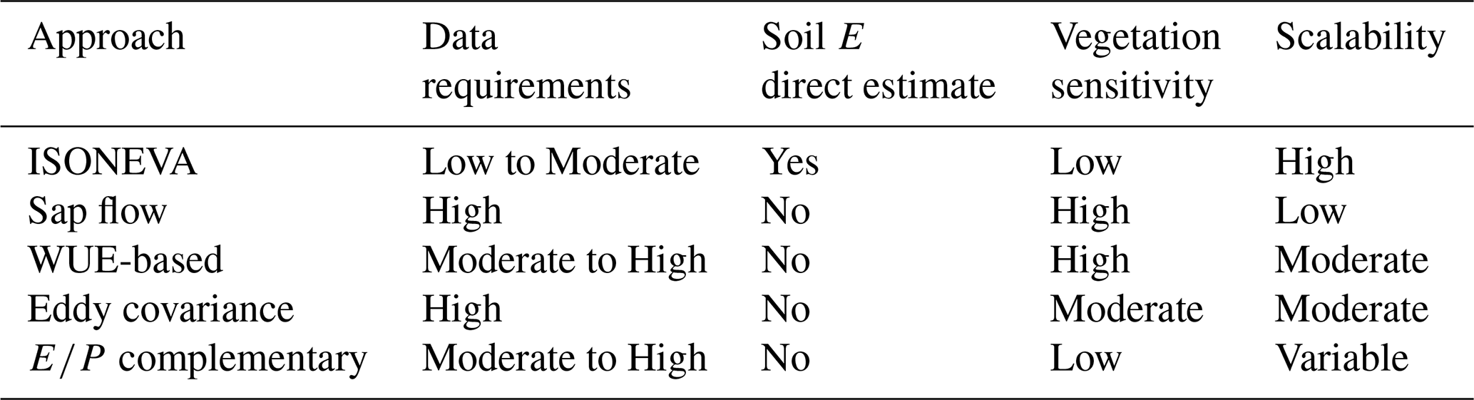
Table 4 Summary comparison of ISONEVA with other common ET partitioning approaches in terms of data requirements, ability to directly estimate soil evaporation, vegetation sensitivity, and scalability.

For spatial scale, virtual experiments showed that ISONEVA achieves the highest accuracy in estimating both $E/P$ and $Q/P$ when the topsoil layer thickness is approximately 0.1 m under humid conditions. This pattern is consistent with the field sampling campaign, where frequent precipitation and irrigation events resulted in $|E/P|<\mathrm{1}$, indicating a humid hydrological regime. The agreement between virtual and field results confirms that the performance of ISONEVA strongly depends on the information content of soil water storage and isotope signals within the control volume. For example, the spike experiment conducted in the field further enhanced the isotopic information in the topsoil. By introducing isotopically enriched water, the experiment amplified the isotopic signal within the soil profile, increasing the contrast between evaporative enrichment and incoming water signals. Such signal amplification has been widely recognized as an effective approach for improving the detectability of isotope-based hydrological processes (Beyer et al., 2020; Dubbert et al., 2022; Penna et al., 2018). Consequently, the strengthened isotopic gradients improved the identifiability of both evaporation and non-evaporative fluxes, even within a relatively thick control volume.

We acknowledge that the optimal depth (∼ 0.1 m) identified in the virtual experiment reflects the specific soil properties (light clay) considered in that setup. This depth should therefore not be interpreted as universally applicable. Nevertheless, under typical field conditions, an effective depth near 0.1 m is fully consistent with the widely adopted practice of using the upper 0.05–0.1 m of soil to represent the evaporating layer, as this zone generally captures the dominant soil-water and isotopic dynamics relevant for evaporation. Broader cross-ecosystem generalization would require multi-site field datasets and represents an important direction for future research. Although ISONEVA performed well in the field test, this evaluation is based on a single lysimeter dataset. Future work should therefore test the method across a broader range of field conditions by integrating additional in situ datasets from different soils, climates, and vegetation systems. Such multi-site evaluations will be necessary to assess the general applicability and robustness of the approach across ecosystems.

4.3 Potential of ISONEVA for ET partitioning

Partitioning ET into E and T remains a central challenge in ecohydrology, especially in arid and semi-arid ecosystems where $E/T$ ratios fluctuate widely in space and time (Rothfuss et al., 2021; Williams et al., 2004). Accurate E estimation provides critical insights into soil–plant–atmosphere interactions, informing sustainable water management and improving understanding of subsurface water dynamics (Good et al., 2015; Sprenger et al., 2016).

Although the ratio $\left|E\right|/(\left|E\right|+\left|Q\right|)$ derived from ISONEVA can theoretically either overestimate or underestimate the true evaporation fraction $E/\mathrm{ET}$, the latter situation is expected to be relatively uncommon under the conditions considered here. In principle, underestimation of $E/\mathrm{ET}$ would occur only when the non-evaporative flux within the topsoil layer exceeds total transpiration (|Q|>T_total). Such situations are most likely associated with short-term infiltration events that generate strong percolation pulses. However, ISONEVA is applied over relatively long integration periods (e.g., monthly), during which transient drainage events typically represent only a minor component of the cumulative water balance (Nimmo et al., 2025). By contrast, transpiration integrates water uptake across the entire rooting zone and often dominates evapotranspiration at ecosystem and global scales. Global syntheses suggest that transpiration commonly accounts for approximately 60 % of total evapotranspiration (Good et al., 2015; Wei et al., 2017). Consequently, over such integration periods the non-evaporative flux within the shallow control volume is generally expected to remain smaller than total transpiration (|Q| ≤T_total), making $\left|E\right|/(\left|E\right|+\left|Q\right|)$ a reasonable conservative upper bound of $E/\mathrm{ET}$.

Importantly, even when interpreted as an upper bound, the estimate remains informative. Because the evaporation fraction $E/\mathrm{ET}$ is inherently constrained between 0 and 1, determining an upper bound effectively reduces the feasible range of ET partitioning. This constraint therefore provides useful diagnostic information about the relative contributions of evaporation and transpiration, particularly in situations where direct transpiration measurements are unavailable or uncertain.

Compared to non-isotope-based ET partitioning methods, such as sap flow (Rafi et al., 2019), eddy covariance (EC) (Paul-Limoges et al., 2020), water-use-efficiency approaches (Yu et al., 2022), and evaporation-to-precipitation complementary methods (Wu et al., 2024; Zhang and Brutsaert, 2021), ISONEVA offers distinct advantages. Its strength lies in minimal data requirements, relying primarily on soil water content and isotopic composition, along with basic meteorological variables. This eliminates the need for detailed vegetation data (e.g., leaf area index, rooting depth) or the extensive calibration datasets often required by meteorological methods (Table 4; Stoy et al., 2019).

However, it should be noted that because $Q/P$ is derived from water balance closure, its value may incorporate residual uncertainties in storage change and precipitation measurements. Independent flux measurements (e.g., sap flow or eddy covariance) would further constrain the physical interpretation of Q. In the present study, validation is conducted under controlled lysimeter conditions, where lateral flow is physically excluded and drainage is directly monitored. Moreover, the water balance of this experimental system has been independently verified in previous studies (Benettin et al., 2021), which increases confidence that the derived $E/\mathrm{ET}$ values are physically reasonable rather than artifacts of mass balance residuals. In natural field applications, additional processes such as deep percolation beyond the monitored layer, capillary rise, or spatial heterogeneity in root water uptake may introduce ambiguity in attributing Q solely to transpiration. Therefore, future studies should integrate independent transpiration measurements or multi-layer flux observations to further constrain the partitioning of non-evaporative fluxes and strengthen the physical interpretation of $E/\mathrm{ET}$ estimates derived from isotope-based inversion.

5 Conclusions

This study introduces ISONEVA, a novel isotope-based framework that explicitly incorporates non-evaporative fluxes to improve soil evaporation estimates within the soil-plant-atmosphere continuum. Traditional steady-state (SS) approaches assume constant water and isotopic conditions that are rarely satisfied in natural soils, whereas non-steady-state (NSS) models often neglect non-evaporative processes such as infiltration or root water uptake, which can introduce mass balance inconsistencies. By explicitly accounting for both evaporative and non-evaporative fluxes, the proposed framework provides a more physically consistent representation of soil water and isotope dynamics. Results from virtual experiments and lysimeter observations demonstrate the feasibility of the approach and illustrate how the framework can constrain the relative contributions of evaporative and non-evaporative fluxes. In particular, the method provides a diagnostic constraint on the evaporation fraction by deriving a physically interpretable bound for $E/\mathrm{ET}$. Such constraints can be valuable for evaluating evaporation dynamics and water partitioning in situations where direct flux measurements are unavailable. Although the current validation is limited to controlled lysimeter conditions, the results highlight the potential of ISONEVA as a complementary tool for isotope-based analyses of soil water fluxes. Future studies should further test the framework across different ecosystems, soil types, and climatic conditions, and may benefit from combining ISONEVA with independent measurements (e.g., sap flow, eddy covariance) or remote sensing data to better evaluate evaporation dynamics at larger spatial and temporal scales.

Appendix A: Derivations of NSS and ISONEVA

A1 NSS

When express the water balance of the topsoil control volume under evaporation-only conditions, where the change in soil water storage ($\frac{\partial V}{\partial t}$) is equal to the evaporation flux E:

$$\begin{array}{}\text{(A1)}& {\displaystyle \frac{\partial V}{\partial t}}=E\end{array}$$

Further, the isotopic mass balance can be written as:

$$\begin{array}{}\text{(A2)}& {\displaystyle \frac{\partial VR}{\partial t}}=E{R}_{\mathrm{E}}\end{array}$$

where VR is the total mass of isotopes in the control volume and ER_E is the isotopic flux associated with evaporation.

By applying the chain rule and combining Eq. (A1), Eq. (A2) can be rewritten as:

$$\begin{array}{}\text{(A3)}& {\displaystyle }V{\displaystyle \frac{\partial R}{\partial t}}+R{\displaystyle \frac{\partial V}{\partial t}}=E\left(AR-B\right)\text{(A4)}& {\displaystyle }V{\displaystyle \frac{\partial R}{\partial t}}=EAR-EB-ER\end{array}$$

Equation (A4) describes the time evolution of soil isotopic composition as a function of the evaporation rate and the isotopic compositions of soil water and evaporated vapor.

Rewriting $v\frac{\partial R}{\partial t}$ in relation to $\frac{\partial \left(\ln f\right)}{\partial t}$ yields:

$$\begin{array}{}\text{(A5)}& V{\displaystyle \frac{\partial R}{\partial t}}={\displaystyle \frac{\partial R}{\partial \left(\ln f\right)}}{\displaystyle \frac{\partial V}{\partial t}}=-EB+\left(EA-E\right)R\end{array}$$

where f is the ratio of final to initial soil water storage.

Consequently, soil isotopic composition R can be written as a function of ln f , combining the water-storage change with isotopic enrichment processes:

$$\begin{array}{}\text{(A6)}& {\displaystyle \frac{\partial R}{\partial \left(\ln f\right)}}+\left(\mathrm{1}-A\right)R=-B\end{array}$$

Solving this first-order linear differential equation leads to Eq. (A7), which provides the analytical solution for the evolution of R.

$$\begin{array}{}\text{(A7)}& R=-{\displaystyle \frac{B}{\mathrm{1}-A}}+f^{-\left(\mathrm{1}-A\right)}\left(R_{\mathrm{0}}+{\displaystyle \frac{B}{\mathrm{1}-A}}\right)\end{array}$$

Note that the partial differential equation like:

$$\begin{array}{}\text{(A8)}& {\displaystyle \frac{\partial y}{\partial x}}+p\left(x\right)y\left(x\right)=q\left(x\right)\end{array}$$

has the analytical solution:

$$\begin{array}{}\text{(A9)}& y=e^{-\int p\left(x\right)\mathrm{d}x}\left(\int q\left(x\right)e^{\int p\left(x\right)\mathrm{d}x}\mathrm{d}x+\text{constant}\right)\end{array}$$

Equation (A9) is used to derive Eq. (A7) from Eq. (A6) (also Eq. A17 from Eq. A16 below).

A2 ISONEVA

Representing the water mass balance of the topsoil control volume, where changes in soil water storage ($\frac{\partial V}{\partial t}$) are determined by precipitation (P), evaporation (E), and percolation (Q):

$$\begin{array}{}\text{(A10)}& {\displaystyle \frac{\partial V}{\partial t}}=P+E-Q\end{array}$$

Then, the isotopic mass balance can be written as:

$$\begin{array}{}\text{(A11)}& {\displaystyle \frac{\partial VR}{\partial t}}=P{R}_{\mathrm{P}}+E{R}_{\mathrm{E}}-QR\end{array}$$

Equation (A11) describes the corresponding isotope mass balance, where VR is the total mass of isotopes stored in the control volume. The terms on the right-hand side represent isotopic inputs from precipitation (PR_P), isotopic enrichment during evaporation (ER_E), and isotopic losses through percolation (QR).

To obtain an equation for the evolution of soil water isotopic composition (R), Eqs. (A10) and (A11) are combined, this leads to Eqs. (A12)–(A14), which express the temporal evolution of R in terms of water fluxes and their isotopic compositions.

$$\begin{array}{}\text{(A12)}& {\displaystyle }V{\displaystyle \frac{\partial R}{\partial t}}+R{\displaystyle \frac{\partial V}{\partial t}}=P{R}_{\mathrm{P}}+E\left(AR-B\right)-QR\text{(A13)}& {\displaystyle }V{\displaystyle \frac{\partial R}{\partial t}}=P{R}_{\mathrm{P}}+EAR-EB-QR-PR-ER+QR\text{(A14)}& {\displaystyle }V{\displaystyle \frac{\partial R}{\partial t}}={\displaystyle \frac{\partial R}{\partial \left(\ln f\right)}}{\displaystyle \frac{\partial V}{\partial t}}=P{R}_{\mathrm{P}}-EB+\left(EA-P-E\right)R\end{array}$$

Like NSS derivations, Eq. (A14) is rewritten in terms of the derivative of R with respect to ln(f), this transformation yields Eq. (A15).

$$\begin{array}{}\text{(A15)}& {\displaystyle \frac{\partial R}{\partial \left(\ln f\right)}}+{\displaystyle \frac{\left(E+P-EA\right)}{P+E-Q}}R={\displaystyle \frac{P{R}_{\mathrm{P}}-EB}{P+E-Q}}\end{array}$$

Finally, Eq. (A15) can be further simplified to Eq. (A16), which is a first-order linear differential equation. It can be solved analytically using Eq. (A9) and results in Eq. (A17), which is the basis of the ISONEVA estimation.

$$\begin{array}{}\text{(A16)}& {\displaystyle \frac{\partial R}{\partial \left(\ln f\right)}}+{\displaystyle \frac{\left(\mathrm{1}+x-Ax\right)}{\mathrm{1}+x-y}}R={\displaystyle \frac{R_{\mathrm{P}}-Bx}{\mathrm{1}+x-y}}\text{(A17)}& {\displaystyle }R={\displaystyle \frac{R_{\mathrm{P}}-Bx}{\mathrm{1}-Ax+x}}+f^{-\frac{\mathrm{1}-Ax+x}{\mathrm{1}+x-y}}\left(R_{\mathrm{0}}-{\displaystyle \frac{R_{\mathrm{P}}-Bx}{\mathrm{1}-Ax+x}}\right)\end{array}$$