A highly generalizable data-driven model for spatiotemporal urban flood dynamics real-time forecasting based on coupled CNN and ConvLSTM

Flooding has become one of the most severe natural hazards in urban areas. Real-time and accurate prediction of flood processes is a crucial approach to mitigate urban flood disasters. Data-driven models based on machine learning methods offer significantly higher computational efficiency than physics-based models and have been widely applied in real-time urban flood simulation. However, most data-driven models target the temporal process of inundation depths at specific sites or the spatial distribution of peak inundation depths, while some models capable of simulating spatiotemporal urban flood inundation often lack spatial generalization capabilities. In this study, we proposed a novel data-driven model to predict the spatiotemporal distribution dynamics of urban inundation depths. The model integrates a ConvLSTM-based component alongside a CNN-based component via a concatenation process, facilitating the extraction of information from both temporal sequences and static geospatial features concurrently. A tiling approach that divides the study area into distinct spatial sub-regions, which serve as independent training samples, was employed during model training to enhance the model's generalization capability. The proposed model was applied to a flood-prone urban area in Macao and compared with a physics-based model. The results show that: (1) the proposed model effectively captures the inundation processes at specific sites, with NSE >0.80 for the majority events, as well as RMSE and MAE values <0.20. (2) The proposed data-driven model demonstrates robust generalization performance, with simulated inundation processes closely aligned with the results of the physics-based model in most regions (mean NSE > 0.70, RMSE < 0.10, MAE < 0.10). Notable discrepancies persist only in localized zones of abrupt terrain variations, particularly near building edges.

1 Introduction

Urban flooding is a critical natural disaster that causes significant loss of life and property damage in urban areas and is expected to increase in both frequency and intensity as a result of global warming and rapid urbanization. In coastal cities, these challenges are intensified by storm surges and rising sea levels, which impose additional burdens on urban drainage systems. Rapid convergence of runoff in urban settings, compounded by intense short-duration rainfall, facilitates the rapid development of urban flooding, thus complicating emergency response efforts (Fu et al., 2023; Wang et al., 2022; Balaian et al., 2024). Consequently, flood forecasting using numerical models has emerged as an essential method to mitigate flood-related losses. In order to underpin effective disaster mitigation strategies, there exists a necessity for precise spatio-temporal processes of inundation depths, thus physics-based hydrodynamic models, which can simulate spatio-temporal flood dynamics in urban areas, have been developed and implemented. However, these models are computationally intensive, leading to low simulation efficiency. When deployed in extensive urban regions, the computation time required by such models may exceed the duration of the events they aim to simulate. Prolonged computation times significantly limit the utility of these models in real-time flood forecasting.

To mitigate the limitations associated with the inefficiency of high-precision, high spatiotemporal resolution flood simulations using physics-based hydrodynamic models, data-driven models have been devised in recent years. These models, characterized by machine learning (ML) or deep learning (DL) methods, infer the input-output relationships from historical data rather than relying on predefined equations or physical laws employed in process-based models for the purposes of prediction or comprehension of complex systems. Upon completion of the training phase, data-driven models are capable of executing a substantial number of simulations within a brief timeframe, all the while preserving a high level of accuracy. Moreover, data-driven models are able to leverage a broader spectrum of diverse datasets more comprehensively. Numerous data-driven models have been employed in the simulation of urban flooding in recent years. For example, Berkhahn et al. (2019) introduced an artificial neural network architecture to forecast peak water levels during flash flood incidents and subsequently evaluated the model in two urban locations. Löwe et al. (2021) introduced a model referred to as U-FlOOD, grounded in the U-NET methodology, to forecast the spatial distribution of the maximum flood depth. Gao et al. (2024) used a one-dimensional convolutional neural network (1D-CNN) to simulate the spatial distribution of the maximum inundation depth in the Tianhe district of Guangzhou City, China. Dai and Cai (2021) simulated water depth dynamics during typhoons in Macao, China, using a backpropagation neural network (BPNN). Zahura et al. (2020) predicted water depth over time in the road segments during rainfall using a Random Forest (RF) model. These studies have shown that data-driven models are capable of effectively simulating urban flood events while also exhibiting significantly higher computational efficiency compared to traditional physics-based models. However, most studies (Hou et al., 2021; Aderyani et al., 2025; Piadeh et al., 2023) that employ data-driven models for urban flood modeling have focused predominantly on the spatial distribution of maximum depths of flooding or inundation processes at specific locations, while limited attention has been paid to the application of data-driven approaches to simulate spatiotemporal inundation dynamics throughout urban flood events. To simultaneously account for the temporal and spatial dependencies of the input data, Shi et al. (2015) integrated the LSTM and CNN models, proposing the convolutional LSTM model (ConvLSTM). They applied the model to precipitation nowcasting, demonstrating its ability to capture spatiotemporal correlations and perform effectively. ConvLSTM-based models have subsequently been widely employed in flood prediction applications due to their effective capacity to extract temporal and spatial information from input features. Specifically, Yang et al. (2024) proposed a ConvLSTM based model to simulate the spatiotemporal dynamics of inundation depths in urban areas and evaluated the model in Huangpu District, Guangzhou city, China. Wang et al. (2024b) introduced a time-guided convolutional neural network by integrating the target time matrix into the input features of the ConvLSTM-based model and evaluated the model in the metropolitan area of Dalian, China. Liao et al. (2025) proposed a ConvLSTM-based architecture that explicitly captures the spatiotemporal distribution of rainfall for flood prediction and compared its performance against that of a 3D CNN model. However, most studies that used ConvLSTM-based models to predict urban inundation depths did not consider static data, such as topography and pipe networks, particularly, or just incorporate static data into input features of ConvLSTM simply. Incorporating static data directly as inputs in ConvLSTM architectures may diminish their influence, as the model inherently prioritizes temporal dynamics over time-invariant attributes. Static data exert a critical influence on urban flooding processes, and neglecting their incorporation would lead to significant adverse impacts on the generalization capability of ConvLSTM-based models.

In order to address the generalization challenges associated with ConvLSTM in the context of urban flooding forecasting, this study proposes a deep learning framework that integrates ConvLSTM and CNN. The ConvLSTM component of the proposed model is utilized to capture the spatial and temporal dependencies inherent in input time series, while the CNN component addresses the spatial dependencies present in static geospatial inputs. To enhance the applicability of the model for real-time flood forecasting and facilitate the incorporation of observed flood data during model execution, an auto-regressive prediction framework is employed, wherein the inundation depth map predicted in the current timestep serves as the input for the subsequent timestep. Furthermore, considering the hydrodynamic characteristics of water flow, the target region is partitioned into multiple segments rather than treated as a singular entity during the training phase, thereby augmenting the model's capacity for generalization. The model was subsequently evaluated in Macao, China.

The organization of the paper is as follows. Section 2 describes the study area; Sect. 3 details the proposed methodology; Sect. 4 presents a comparative analysis of the simulation results between the proposed data-driven model and the physics-based model. Section 5 discusses the limitations of the proposed model, and Sect. 6 provides a concise conclusion.

2 Study Area and Data

2.1 Study Area

The research is concentrated in the western sector of the Macao Peninsula (Fig. 1). This region is characterized by a subtropical climate and is influenced by an oceanic monsoon system, with an average annual precipitation of 1966.6 mm. It is highly urbanized and characterized by a low-lying topography with the lowest elevation only 1.4 m above sea level and an average elevation of approximately 2 m. Due to its climatic and geographical characteristics, this region suffers from floods induced by extreme precipitations and storm surges. The 4.06 km² region was ultimately selected as the focus of the study, based on the topographic distribution and drainage systems, as it is the site most prone to historical inundation events in Macao (Dong et al., 2024).

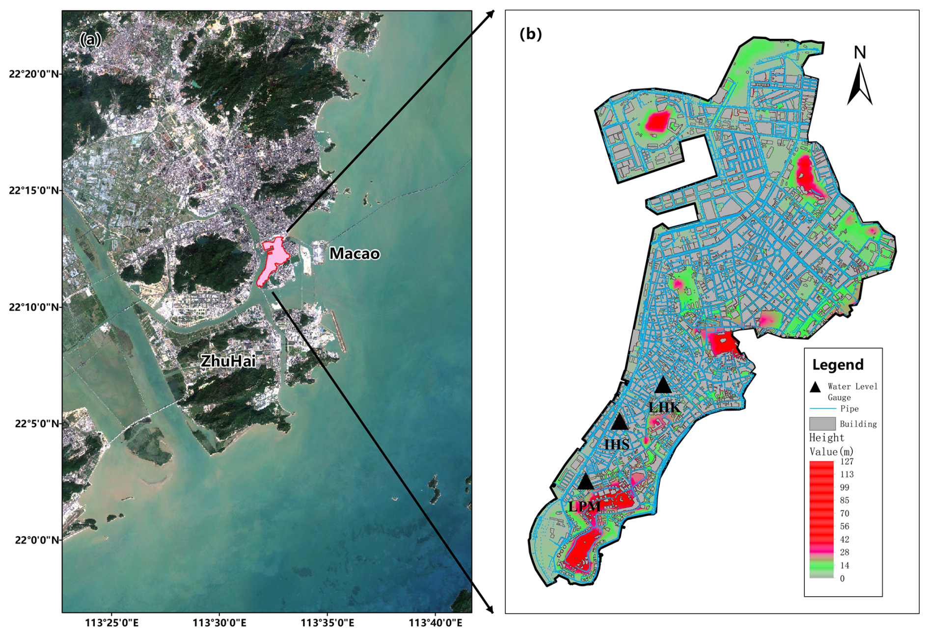
Figure 1 (a) Location of the study area, outlined by the pink polygon. Imagery © 2023 Sentinel-2, Map data © 2023 European Union/ESA/Copernicus. (b) High-resolution digital elevation model (DEM) with building footprints, drainage pipelines, and three water-level monitoring stations.

2.2 Data

2.2.1 Geospatial data

Digital Elevation Model (DEM) data, with a spatial resolution of 2 m, along with the drainage network (Fig. 1) and the building distribution information, were obtained from the Macao Cartography and Cadastre Bureau. The elevations in the DEM at building sites increased by 5 m to account for the impediment effect of buildings on surface water flow. All data were verified on the basis of satellite imagery and field investigation. The DEM, drainage network, and building distribution data were first compared with high-resolution satellite imagery to ensure accuracy. For areas where the satellite imagery was unclear, field surveys were conducted to validate the data on-site and address any discrepancies.

2.2.2 Rainfall

In this study, two types of rainfall data were used, including historical observed data and designed data, to consider more rainfall conditions. The hourly rainfall records for the Dapaotai station, covering the period from 2000 to 2022, were obtained from the Macao Meteorological and Geophysical Bureau. The designed rainfall was formulated by integrating rainfall patterns and intensities. Rainfall patterns were identified by classifying historical rainfall records into seven prototypical patterns, preserving the three most frequently occurring patterns. The seven typical rainfall patterns are shown in Fig. 2. The patterns I, II, and III exhibit a unimodal distribution, with peaks occurring in the early, middle, and late stages, respectively. The pattern IV is characterized by a uniform distribution, while patterns V, VI, and VII show a bimodal distribution (Chen et al., 2015). The predominant rainfall patterns within the study area are the pattern I, the pattern III and the pattern IV, contributing to 41.3 %, 37.2 %, and 13.2 % of the total occurrences, respectively. Therefore, these three rainfall patterns were selected as the designed rainfall patterns. Rainfall intensities were computed based on equations provided by the Macao Meteorological and Geophysical Bureau. The equation is as follows.

$$\begin{array}{}\text{(1)}& I=a{t}^b\end{array}$$

where I represents the intensity of the rainfall (mm h⁻¹); t represents the duration of the rainfall (min); a and b are experimental parameters, which can be obtained from the Macao Regulations on Water Supply and Drainage (Zhang et al., 2024).

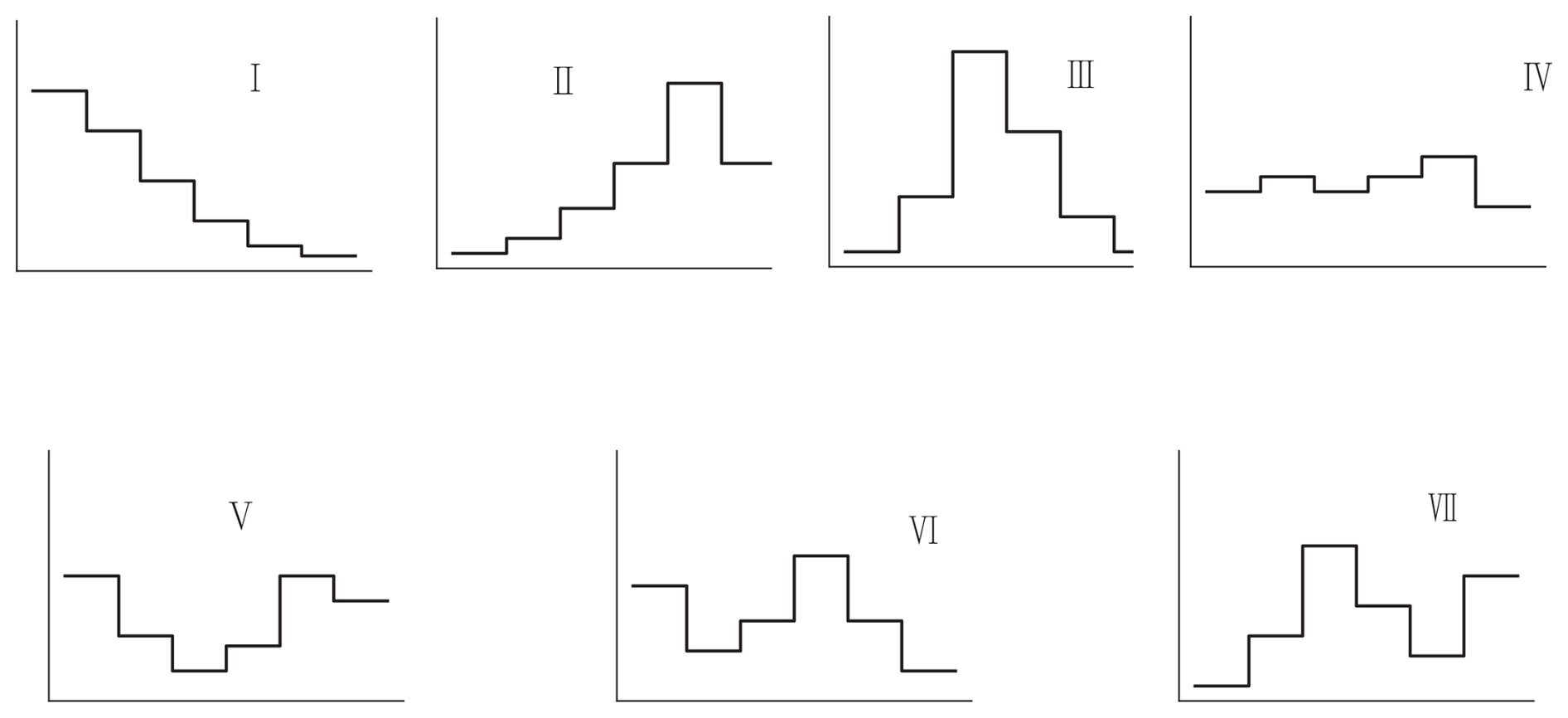
Figure 2 Seven typical rainfall patterns. The horizontal axis represents time, and the vertical axis represents rainfall intensity.

Urban flooding is mainly caused by short, intense rainfall, so a 6 h duration was chosen for the designed rainfall. The designed rainfall amounts for return periods of 10, 20, 50, and 100 years were used to cover most of the rainfall intensities observed in this region. As a result, a total of 12 rainfall scenarios were devised through the integration of three distinct rainfall patterns with four different return periods. Given the relatively small size of the study area, it was assumed that the rainfall would be uniformly distributed throughout the entire region.

2.2.3 Storm tide

Macao Peninsula is frequently affected by storm surges. Due to the low-lying topography, storm surges negatively impact the drainage capacity of the study area, thereby exacerbating flooding events when they coincide with heavy rainfall. Consequently, it is imperative to incorporate the tidal process in the analysis of flooding within the study area. In this study, the designed tidal process lines of 5 warning levels derived by Zhang et al. (2024) were used. The designed tidal process lines are shown in Fig. 3.

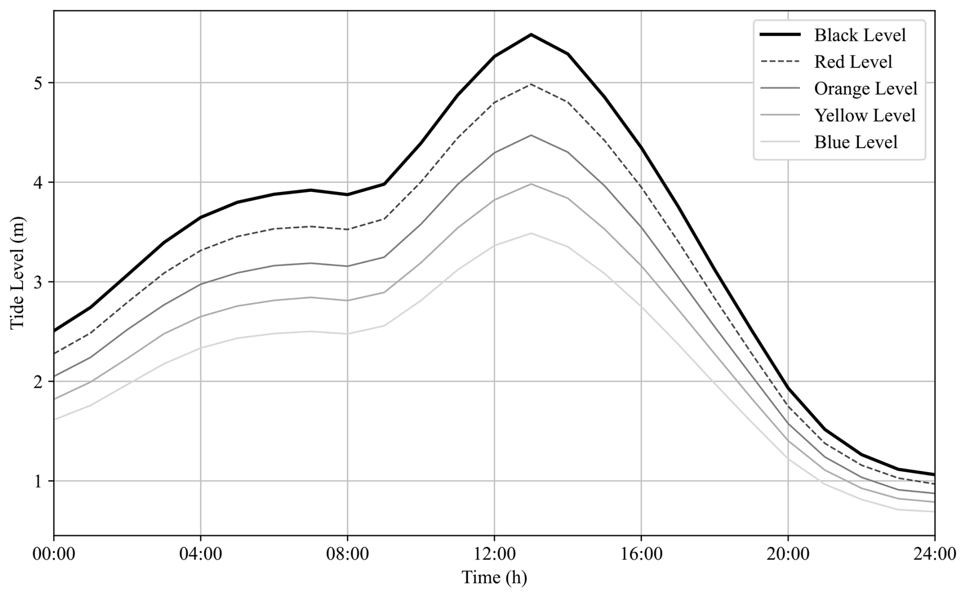
Figure 3 The designed tidal process lines. Temporal variations in tide level (metres) are shown for five threshold processes (black, red, orange, yellow, and blue lines), illustrating daily tidal fluctuations used in model simulations.

2.2.4 Synthetic compound scenarios

The integration of rainfall events and tidal process lines is essential to accurately represent the combined impact of precipitation and storm surges. To integrate rainfall events with tidal process lines in different temporal phases and warning levels, this study proposes the following method for combination. For each rainfall event, a tidal process line is initially selected at random from among the five warning levels. Subsequently, a 6 h interval is randomly determined from the chosen tidal process line to be integrated with the rainfall event. The combination process was conducted thrice for each rainfall event to augment the sample variability.

3 Methodology

The data flow and workflow of this study are shown in Fig. 4. Initially, the dataset was meticulously prepared. The input features for the proposed data-driven model were rigorously selected and classified into static and dynamic categories based on their temporal invariance. Urban flood inundation, which constitutes the output of the proposed data-driven model, was simulated using a physics-based hydrodynamic model, in light of the relative scarcity of inundation depth monitoring data. The dynamic and static input features, along with the corresponding simulated water depths, were paired and randomly divided into training and testing datasets. Subsequently, the proposed data-driven model was trained and its accuracy and computational efficiency was evaluated.

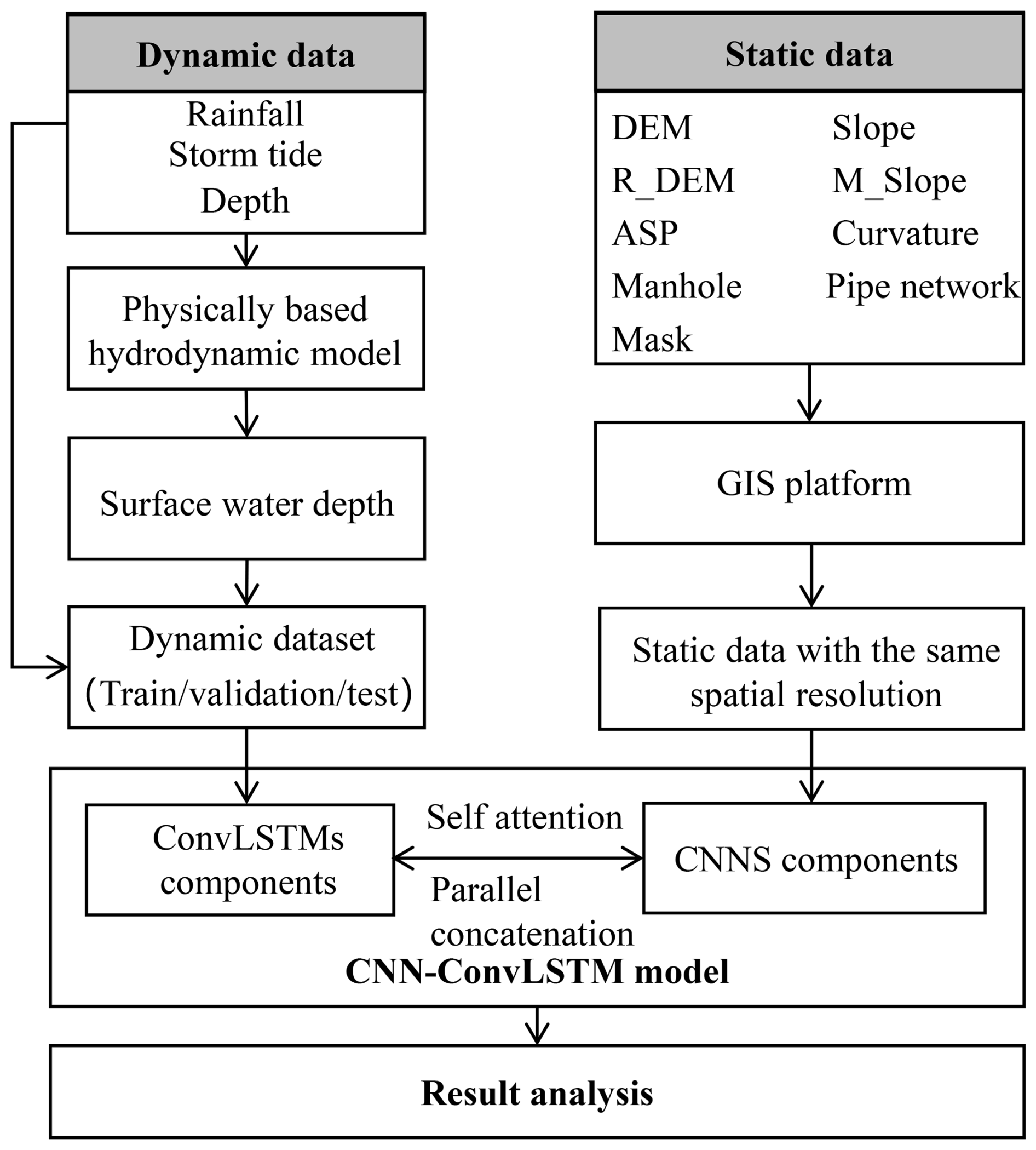
Figure 4 Data flow and workflow of the CNN–ConvLSTM framework. Dynamic data (rainfall, storm tide, simulated water depth) and static data (DEM and terrain features) are preprocessed and integrated into the model through ConvLSTM and CNN branches, respectively. The fused network predicts surface water depth for further analysis.

3.1 Physics-based Hydrodynamic Model

We developed a hydrodynamic model capable of simulating two-dimensional surface flows, one-dimensional flows from the pipe drainage network and the interactions between surface flows and flows from the pipe drainage network. The two-dimensional module solves the Saint-Venant equations using finite-volume methods based on triangular meshes (Anastasiou and Chan, 1997). The module effectively addresses dry-wet alternation, crucial in urban flooding. The EXTRAN module of the SWMM model was used to simulate flows in pipe drainage networks. It simulates the drainage system as links and nodes, enabling the simulation of parallel or looped pipe networks, as well as weirs, orifices, pumps, and system surcharges. The module assumes that the flow within a link is uniform and that the water surface at the node is continuous, resolves the one-dimensional Saint-Venant equations in link-node structures by employing the Predictor-Corrector Iterative method (Rossman and Huber, 2017). The interaction between surface flows and flows in pipe drainage networks is simulated using weir flow formulas (Wang et al., 2024a). The rainfall-runoff process is modeled using the Horton infiltration method. This empirical formula posits that, as the soil reaches saturation, the infiltration rate decreases exponentially from an initial maximum value to a steady minimum rate (Gülbaz et al., 2020; Beven, 2004).

The hydrodynamic model for the study area was built in our previous research. Detailed information on the model can be found in Dong et al. (2024). The performance of the hydrodynamic model was verified by comparing the simulated inundation depths with the waterlogging points observed during Typhoon Mangkhut. The Nash efficiency coefficients for the observed points exceed 0.75. Therefore, the model can be considered capable of accurately reflecting the relationship between rainfall and waterlogging in the area. Training the DL model with the simulation results from hydrodynamic models is a reasonable approach.

3.2 CNN-ConvLSTM Coupled Model

The proposed model is based on ConvLSTM, which is effective in capturing spatiotemporal correlations in multidimensional time series (Shi et al., 2015). However, ConvLSTM has limitations in handling static features such as geospatial information, which are essential to simulate the characteristics of urban floods. The LSTM components of the model, such as input and forget gates as well as memory cells, become superfluous in scenarios devoid of temporal dynamics, thereby introducing unwarranted computational overhead and increasing parameterization, which exacerbate the risk of overfitting. The necessity to process even a single-step input through temporally unfolded operations further results in resource inefficiency when compared to models focused solely on spatial data, like CNNs (Wang et al., 2024b). Moreover, instability during training can occur, as gradient propagation within LSTM modules presents difficulties in adapting to static data absent of sequential dependencies. Consequently, the hybrid architecture of ConvLSTM is excessively complex for static contexts, where simpler models, such as CNNs or MLPs, demonstrate greater efficiency and performance by eliminating redundant temporal mechanisms (Wang et al., 2025). To enhance the efficiency of processing static data, we propose a novel hybrid architecture that integrates ConvLSTM and CNN in parallel. The temporal dynamic information and static features are separately processed by ConvLSTM cells and CNN cells, integrated through feature aggregation, and subsequently decoded to capture the spatiotemporal flood processes.

3.2.1 Convolutional neural network

Convolutional Neural Networks (CNNs) are deep learning models for grid-structured data such as images. Widely used in fields such as computer vision and remote sensing (Lecun et al., 1998; Krizhevsky et al., 2017). In hydrology and flood modeling, CNNs have demonstrated strong capability in capturing terrain-related spatial dependencies and spatial heterogeneity in distributed parameters (Sit et al., 2020). CNNs can learn spatial feature hierarchies efficiently. They offer parameter efficiency through weight sharing in convolutional layers, reducing learnable parameters compared to fully connected networks. CNNs ensure translation invariance, enabling robust feature extraction despite data shifts. By automatically capturing local and global patterns, they excel in tasks like image classification and semantic segmentation. Techniques like pooling and dropout improve computational efficiency and reduce overfitting, enhancing generalization across datasets. In this study, two-dimensional CNNs are used to handle static features such as DEM and the spatial distribution of drainage systems.

3.2.2 Convolutional Long Short-Term Memory network

Convolutional Long Short-Term Memory (ConvLSTM) is a specialized recurrent neural network architecture designed to model spatiotemporal correlations in sequential data with spatial structure. Unlike traditional LSTM, which processes temporal dependencies in vectorized sequences, ConvLSTM replaces fully connected operations with convolutional gates, enabling it to simultaneously capture local spatial patterns and long-range temporal dynamics. This design inherently preserves the spatial topology while capturing temporal dependencies, enabling synergistic learning of localized spatial patterns and long-range temporal dynamics. Compared to architectures that separately stack CNNs and LSTMs, ConvLSTM achieves superior parameter efficiency through convolutional kernel sharing and supports hierarchical multiscale spatiotemporal feature extraction via deep stacking. Its state-of-the-art performance in applications such as precipitation nowcasting and traffic flow prediction underscores its capability to model complex spatiotemporal interactions, establishing it as a benchmark for grid-structured sequential data (Ahmad et al., 2023; Zhang et al., 2017; Lu et al., 2024). Critically, this integrated approach eliminates the need for hand-crafted feature engineering, enhancing generalization across diverse domains. In this study, Time series data, including precipitation and inundation depth, are incorporated as inputs to the ConvLSTM branch for spatiotemporal modeling of flood dynamics. The core operations of a ConvLSTM cell are defined as:

$$\begin{array}{}\text{(2)}& {\displaystyle }{i}_t=\mathit{\sigma }(W_{xi}*x_t+W_{hi}*h_{t-\mathrm{1}}+W_{ci}\circ c_{t-\mathrm{1}}+b_i)\text{(3)}& {\displaystyle }{f}_t=\mathit{\sigma }(W_{xf}*x_t+W_{hf}*h_{t-\mathrm{1}}+W_{cf}\circ c_{t-\mathrm{1}}+b_f)\text{(4)}& {\displaystyle }{c}_t=f_t\circ c_{t-\mathrm{1}}+i_t\circ \tanh (W_{xc}*x_t+W_{hc}*h_{t-\mathrm{1}}+b_c)\text{(5)}& {\displaystyle }{o}_t=\mathit{\sigma }(W_{xo}*x_t+W_{ho}*h_{t-\mathrm{1}}+W_{co}\circ c_t+b_o)\text{(6)}& {\displaystyle }{h}_t=o_t\circ \tanh \left(c_t\right)\end{array}$$

where * denotes convolution, ∘ represents the Hadamard product, and σ is the sigmoid function. $i_t,f_t,o_t$ represent input, forget, and output gates controlling information flow, respectively. x_t denotes the input tensor at time step t. h_t and c_t denote hidden state tensor and cell state tensor at time t. W_x* and W_h* denote convolutional kernels. W_c* denotes kernel for peephole connections. b_* denotes bias terms for each gate. tanh denotes hyperbolic tangent activation function.

3.2.3 Inputs and outputs

The presented model's input features encompass static attributes, which correspond to fixed spatial characteristics, along with spatiotemporal dynamic attributes that signify meteorological and hydraulic variables.

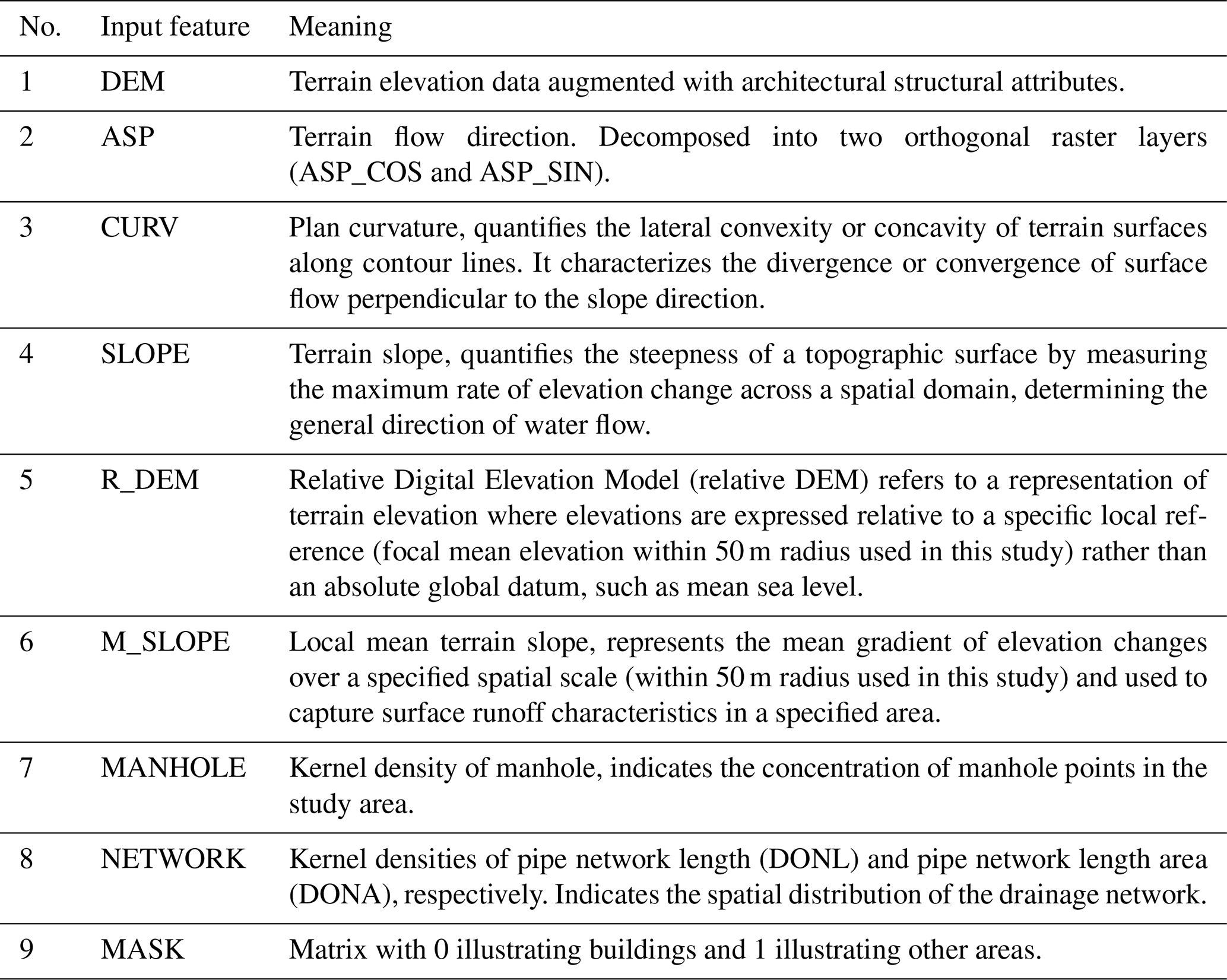
According to the research of Gao et al. (2024), DEM, ASP, CURV, SLOPE, R_DEM, M_SLOPE, TWI, MANHOLE, and NETWORK are sensitive to urban inundation depths and were selected as static input features. The definitions of these static features are provided in Table 1. Among these static features, DEM, ASP, R_DEM, CURV, SLOPE, and M_SLOPE serve as indicators of local terrain deformations linked to surface flow convergence. TWI functions as an integrative index that reflects the potential for soil moisture saturation within the study area. Meanwhile, MANHOLE and NETWORK denote the distribution of drainage systems and suggest levels of urbanization to a certain degree. The correlation analysis conducted by Gao et al. (2024) revealed that R_DEM and TWI exhibit stronger correlations with inundation depth. However, since the study area is an urban region where terrain variations are abrupt and highly discontinuous, the TWI is not applicable. Therefore, this indicator was excluded from the set of sensitivity indicators. The more pronounced correlation of R_DEM compared to DEM indicates that pluvial flooding is generally attributed to relative topographic depressions rather than absolute elevation. Furthermore, the selected variables, with the exception of CURV and SLOPE, exhibit no significant multicollinearity. Nevertheless, these two variables represent distinct topographic attributes. CURV reflects the characteristics of the accumulation of regional surface water, while SLOPE refers to the characteristics of regional surface drainage. Consequently, both variables were incorporated into the study. Furthermore, a building mask (MASK) was incorporated into the input features, acknowledging the significant impact of buildings on hydrological flow within urban environments. The analysis of skewness and kurtosis revealed that certain datasets present right-skewed, long-tailed distributions. Therefore, suitable transformations were implemented to mitigate the effects of outliers. The selection of transformation methods was based on skewness, kurtosis, and the occurrence of negative values in the datasets. A square root transformation was applied to DEM, M_SLOPE, MANHOLE, and NETWORK, whereas a cube root transformation was implemented for R_DEM, SLOPE, and CURV. The selected variables were normalized to a range of 0 to 1 to ensure consistent feature scaling, stabilize training, speed up convergence, and enhance model generalization. The static input features can be expressed as

$$\begin{array}{ll}{\displaystyle }{X}_{\mathrm{sta}}=& {\displaystyle }(\mathrm{DEM},\mathrm{ASP},\mathrm{CURV},\mathrm{SLOPE},\text{R\_DEM},\\ \text{(7)}& {\displaystyle }& {\displaystyle }\text{M\_SLOPE},\mathrm{MANHOLE},\mathrm{NETWORK},\mathrm{MASK})\end{array}$$

Table 1 Definition and Description of Static Input Features which is related to terrain and drainage network characteristics.

Rainfall, tide level, and inundation dynamics are incorporated as time-varying forcing input to the model. To improve the efficacy of the model in real-time urban flood forecasting and to effectively incorporate historical information, rainfall and tide level from the three previous hours to the following 1 h, in conjunction with the inundation depth of the last three hours, are employed to predict the inundation distribution for the following hour. The rainfall distribution is obtained using the inverse distance weighting interpolation based on observed station data, while the inundation distribution is extracted from the model's output of the preceding step. The dynamic input features can be expressed as

$$\begin{array}{}\text{(8)}& X_d=(P^{t-s:t+\mathrm{1}},T^{t-s:t+\mathrm{1}},D^{t-s:t})\end{array}$$

where P, T, and D represent rainfall, tide level, and inundation water depths, respectively. The number of historical temporal intervals (s) can be considered a hyperparameter within the model, as it is potentially influenced by the scale of the study area and the prevailing climate conditions. Considering that the study area is relatively small and its rainfall-runoff process is rapid, in this study the value of s was set to 3 h.

The model outputs the estimated water depth at time t+1. The output is used to update the dynamic input feature D^t+1 for the subsequent iteration, which directs the model to forecast the inundation distribution in a recursive way. This framework enables real-time data assimilation of inundation depths during model execution by integrating observational measurements.

3.2.4 Tiling strategy

To enhance the spatial generalization capability of the model and reduce GPU memory requirements, the study area was divided into a series of square tiles, each of which was treated as an independent training sample. During the partitioning process, an overlap of less than 10 % of the total extent of the study area was introduced in each respective direction to enhance the sample coverage and ensure smoother spatial continuity between adjacent tiles. The tiling strategy is physically reasonable, as urban areas are typically organized into a series of drainage sub-catchments whose hydrological characteristics are primarily governed by internal factors such as local topographic deformations and drainage network configuration. Different sub-catchments are relatively independent from one another, making this partitioning approach consistent with the physical structure of urban drainage systems. The tile size was determined by selecting the optimal configuration based on the performance of the model with different tile sizes.

3.2.5 Model structure

The structure of the CNN-ConvLSTM coupled model is shown in Fig. 5. The model has two components, including the ConvLSTM-based component and the CNN-based component. The ConvLSTM-based component employs an encoder-decoder architecture. The encoder consists of a single ConvLSTM2D layer with 32 convolutional kernels (3 × 3) and LeakyReLU activation, yielding a 100 × 100 × 32 spatiotemporal feature tensor. The decoder mirrors the encoder's structure to reconstruct spatiotemporal dependencies. A batch normalization layer is incorporated between the encoder and the decoder to accelerate the convergence of the model by stabilizing the propagation of the gradient. The input of the ConvLSTM-based component is a temporal sequence comprising rainfall, tidal level, and depth of inundation in four continuous time intervals, structured as a 4 × 100 × 100 × 3 tensor (timesteps × height × width × channels). The CNN-based component comprises three 2D convolutional layers. The initial layer employs 64 kernels (3 × 3) to extract primary spatial features, while the subsequent two layers utilize 32 kernels (3 × 3) each to compress channels and enhance discriminative power through hierarchical feature refinement. The CNN module processes a single-sample input tensor of dimensions 1 × 100 × 100 × 9, comprising nine categories of geographic information data (e.g., digital elevation models [DEM], drainage networks), and generates an output tensor of size 1 × 100 × 100 × 32, which maintains spatial alignment with the ConvLSTM branch for subsequent feature fusion. The outputs of the two branches are merged by a concatenation operation, forming a fused tensor of dimensions 1 × 100 × 100 × 64. Finally, a 3D convolutional layer employing 3 × 3 × 3 kernels compresses the channel dimension to generate the water depth prediction map (1 × 100 × 100 × 1).

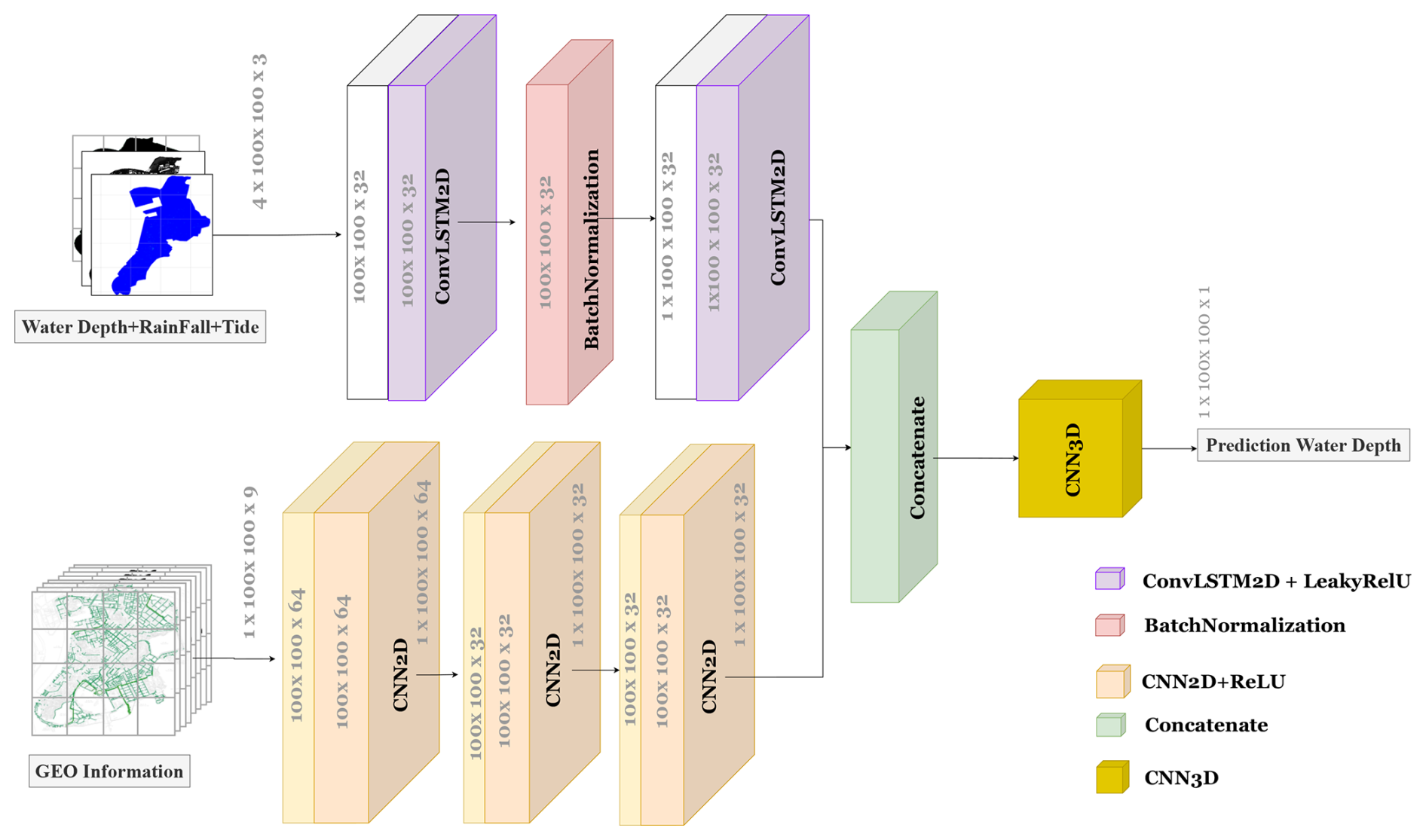
Figure 5 The architecture of the CNN-ConvLSTM coupled model. The model consists of two components: the ConvLSTM component, which employs a two-layer ConvLSTM encoder-decoder architecture to process dynamic inputs such as rainfall, tidal levels, and water depth data, and the CNN component, which consists of three 2D convolutional layers to extract geographic features from static inputs. The outputs of both components are fused by concatenation and then passed through a 3D convolutional layer to generate the water depth prediction.

3.3 Data-driven Model Setup

3.3.1 Training strategy

A multistep-ahead loss function ℒ was used to stabilize the model output, measuring the accumulated error over consecutive time steps. The function is defined as

$$\begin{array}{}\text{(9)}& \mathcal{L}={\displaystyle \frac{\mathrm{1}}{H}}\sum _{\mathit{\tau }=\mathrm{1}}^H\Vert {\widehat{D}}^{t+\mathit{\tau }}-D^{t+\mathit{\tau }}{\Vert }_{\mathrm{2}}\end{array}$$

where H refers to the number of consecutive prediction time instants; ${\widehat{D}}^{t+\mathit{\tau }}$ and D^t+τ are the estimated and observed inundation depths, respectively. The loss function computes the average root mean squared error (RMSE) across all prediction iterations. This process enables the model to refine its predictions autonomously and enhances its capability to produce accurate output even when initial predictions are slightly inaccurate, thus enhancing its robustness. To improve training speed and stability, we employ a progressive training strategy (curriculum learning strategy), initially calibrating the model over a restricted set of forecast horizons and incrementally expanding the prediction window to H (Bentivoglio et al., 2023). The progress of the training strategy is shown in Fig. 6.

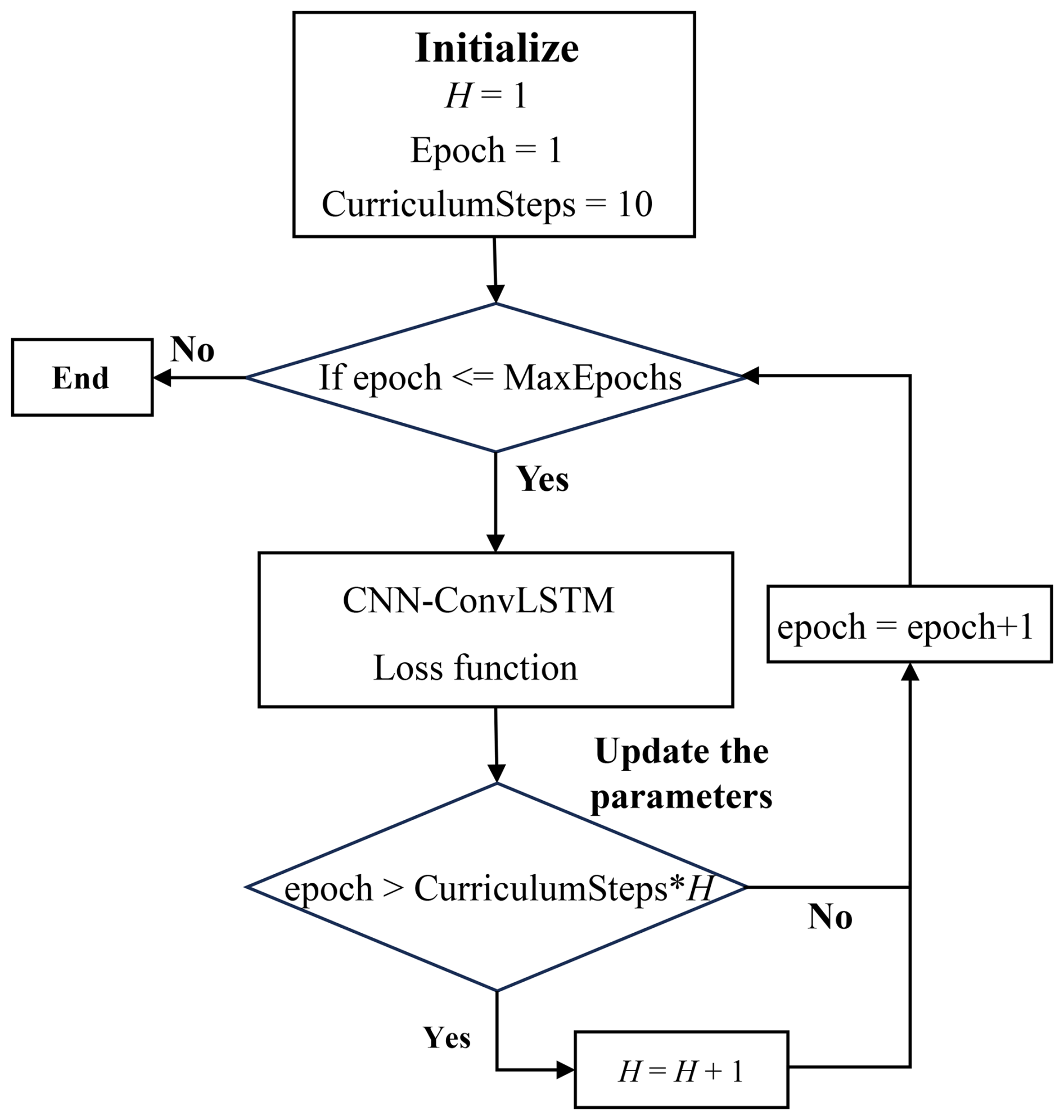
Figure 6 Workflow of curriculum learning strategy. The workflow includes initialization, progressive training stages across epochs, and parameter updates designed to improve convergence and predictive stability.

As described in the section on inputs and outputs, the data pairs employed to train the data-driven model were extracted from rainfall events and their corresponding inundation simulations of the physics-based hydrodynamic model using a fixed time window. Therefore, it is unnecessary to account for the effects of rainfall patterns and return periods particularly, when preparing the training and testing datasets. 80 % of the dataset was randomly allocated for model training, while the remaining 20 % was reserved for model testing. The divide strategy is based on rainfall events, rather than random sampling of the entire dataset, to prevent data leakage across temporal sequences. To ensure the model's generalization capability, the test set was strictly excluded from the training process, and 15 % of the training set was allocated as a validation set for hyperparameter tuning and early stopping.

3.3.2 Evaluation metrics

The efficacy of the proposed CNN-ConvLSTM model was assessed by comparing the water depths forecasted by the CNN-ConvLSTM model with those simulated by the physics-based hydrodynamic model. The assessment used various performance metrics, including the Nash–Sutcliffe efficiency (NSE) (Nash and Sutcliffe, 1970), the root mean square error (RMSE) (Willmott, 1981), the mean absolute error (MAE) (Hyndman and Koehler, 2006), and the critical success index (CSI) (Schaefer, 1990). NSE evaluates the predictive skill of the model relative to the mean of the observations, with values ranging from −∞ to 1, where 1 represents the best performance. RMSE and MAE assess the average prediction errors, with RMSE emphasizing larger errors and MAE reflecting the overall error. Both RMSE and MAE range from 0 to ∞, with the best value being 0. In this study, the units of RMSE and MAE are meters. CSI evaluates the model's ability to accurately distinguish between flooded and non-flooded areas, with values ranging from 0 to 1, where 1 indicates the best performance. The definitions of these metrics are as follows.

$$\begin{array}{}\text{(10)}& {\displaystyle }\text{NSE}=\mathrm{1}-{\displaystyle \frac{{\sum }_{t=\mathrm{1}}^T{\left(d^t-{\widehat{d}}^t\right)}^{\mathrm{2}}}{{\sum }_{t=\mathrm{1}}^T{\left(d^t-\stackrel{\mathrm{‾}}{d}\right)}^{\mathrm{2}}}}\text{(11)}& {\displaystyle }\text{RMSE}=\sqrt{{\displaystyle \frac{\mathrm{1}}{n}}\sum _{i=\mathrm{1}}^n(d_i-{\widehat{d}}_i{)}^{\mathrm{2}}}\text{(12)}& {\displaystyle }\text{MAE}={\displaystyle \frac{\mathrm{1}}{n}}\sum _{i=\mathrm{1}}^n|d_i-{\widehat{d}}_i|\end{array}$$

where d_i and ${\widehat{d}}_i$ represent observed and predicted water depth on the ith grid; d^t and ${\widehat{d}}^t$ represent observed and predicted water depth of time t; n denotes the number of predicted values.

$$\begin{array}{}\text{(13)}& \text{CSI}={\displaystyle \frac{\text{TP}}{\text{TP}+\text{FN}+\text{FP}}}\end{array}$$

where TP (True Positive) signifies the count of wet grids accurately predicted by the proposed data-driven model; FP (False Positive) refers to the count of dry grids mistakenly identified as wet; FN (False Negative) represents the number of grids mistakenly predicted to be dry.

4 Results

4.1 Determination of the tile size

Considering both the extent of the study area and the typical scale of urban drainage sub-catchments, we evaluated tile sizes ranging from 50 × 50 to 300 × 300 grid cells, with an interval of 50 cells between configurations. Each grid cell corresponds to a 2 × 2 m spatial resolution. As illustrated in Fig. 7, this analysis examines how increasing the tile size influences model accuracy and stability. Overall, the simulations across all tile-size configurations performed well, achieving a mean Nash–Sutcliffe efficiency (NSE) greater than 0.7, a mean absolute error (MAE) below 0.01, and a root mean square error (RMSE) below 0.12. However, the average NSE exhibited a rising–falling trend, while the MAE showed the opposite declining–rising pattern, with both metrics reaching their optimal values when the tile size was 100 × 100 grid cells. Accordingly, this configuration was adopted for subsequent experiments. These results indicate that tile size exerts a measurable influence on model performance. The observed variation can be attributed to edge effects between adjacent tiles: When the tile size approximates the typical scale of the smallest urban drainage sub-catchment, each tile functions relatively independently, with limited intertile flux exchange. As a result, boundary effects are minimized and simulation accuracy is enhanced.

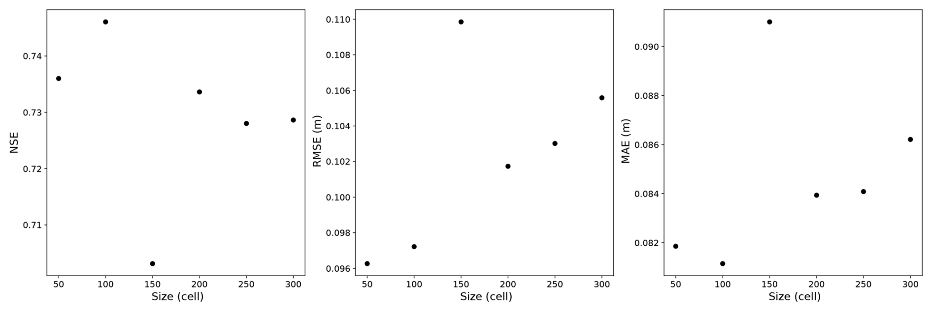
Figure 7 Sensitivity of model performance to tile size (50–300 cells), with the best overall scores at 100 cells. NSE (left), RMSE (middle), and MAE (right) are shown as functions of tile size. Each black marker corresponds to one model run for a given tile size evaluated on the same dataset. Higher NSE and lower RMSE/MAE indicate better performance.

4.2 Performance of data-driven model in water depth simulation at flood-prone locations

Water depth predictions from the CNN-ConvLSTM model were compared with the physics-based model in three flood-prone locations, LHK, IHS, and LPM, which were used to calibrate the physics-based model in our previous study (Dong et al., 2024). Inundation processes corresponding to five rainfall events at each location were randomly selected to assess the capability of the proposed data-driven model in replicating the inundation dynamics simulated by the physics-based model. As shown in Fig. 8, the water depth processes predicted by the data-driven model for the selected rainfall events exhibited a strong consistency with the simulations generated by the physics-based model. In five randomly selected rainfall events, the NSE values at stations IHS and LPM consistently exceeded 0.80, while station LHK also showed NSE values above 0.80 in all but one event, which had an NSE of 0.75. Among the 15 rainfall events evaluated, 13 exhibited both RMSE and MAE below 0.20, with more than half exhibiting values below 0.10 for both metrics. This demonstrates that the proposed data-driven model effectively captures the dynamics of water depth in flood-prone locations, capturing key temporal patterns of inundation processes. The relatively lower NSE value (0.75) occurred under the combined condition of high tide levels and Pattern I heavy rainfall events. The training dataset primarily consisted of observed rainfall–tide combinations, supplemented by a small number of designed scenarios. Since the specific combination of high tide and Type I rainfall accounted for only a small proportion of the training samples, the model exhibited relatively poorer simulation performance under this condition.

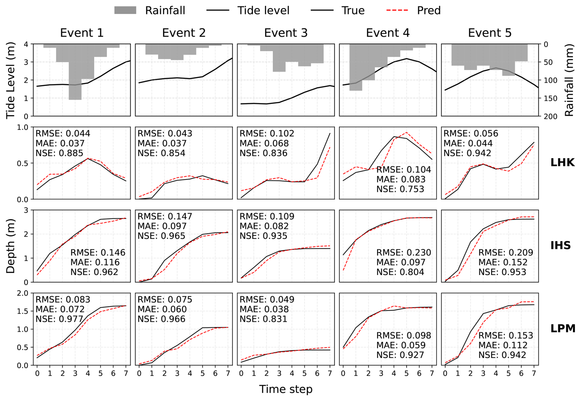
Figure 8 Observed and predicted water depth processes at three flood-prone locations (LHK, IHS, and LPM) during five rainfall events. Tide level and rainfall are shown in the top row, followed by time series of observed and predicted water depths at each site. Model performance for each event is quantified using RMSE (m), MAE (m), and NSE.

4.3 Performance of data-driven model in simulating water depth spatiotemporal dynamics

The mean values of NSE, RMSE, and MAE across the study area were 0.83, 0.08, and 0.05, respectively, demonstrating the efficacy of the proposed data-driven model in simulating inundation processes from a basin-wide perspective. In addition, CSI was recorded as 0.83, indicating that the model detects the presence of flooding in the study area efficiently. To evaluate the model’s capability in capturing the spatiotemporal dynamics of inundation water depths, the mean values of NSE, RMSE, and MAE across all rainfall events, together with the corresponding station-based boxplots, are presented in Fig. 9.

Overall, most regions exhibit mean NSE values above 0.7, with RMSE and MAE consistently below 0.10 m, indicating robust performance of the proposed CNN–ConvLSTM model in reproducing the spatiotemporal patterns of inundation depths. Larger discrepancies between the data-driven and physics-based simulations are mainly concentrated in narrow inter-building zones, where abrupt terrain changes and complex urban micro-topography limit the model’s ability to accurately capture flow redistribution. The boxplots further show that nearly 75 % of the NSE values exceed 0.80, while most RMSE and MAE values remain below 0.10 m across all locations and rainfall events. At the station level (bottom row), the three locations show consistently high accuracy (median NSE ≈ 0.95) but different dispersion. LHK exhibits the tightest interquartile range and the smallest errors, indicating the most stable performance. IHS displays the largest variability – with wider IQRs and longer upper whiskers in both RMSE and MAE – suggesting that several events are harder to reproduce there (peak errors approaching 0.20–0.25 m). LPM lies between LHK and IHS: typical errors remain low, although a few events show increased deviations. As discussed in Sect. 4.2, the RMSE and MAE variability at these two locations primarily stems from the under-representation of concurrent high-tide and Pattern-I heavy-rainfall events in the training data, leading to weaker simulation performance under such conditions. These results confirm the model’s strong capability to generalize inundation dynamics over diverse spatial and hydrometeorological conditions. Note that grids with water depths below 0.20 m were excluded from evaluation, consistent with the model’s focus on flooding processes.

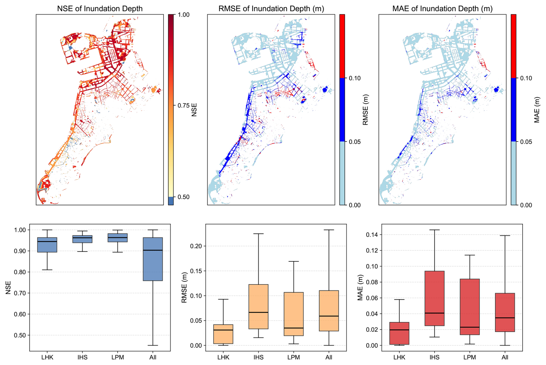
Figure 9 Spatial distribution (top row) and station-based boxplots (bottom row) of the evaluation metrics for inundation water depth. The first row shows the spatial distribution of the mean NSE, RMSE, and MAE across all rainfall events, while the second row presents the boxplots at three representative locations (LHK, IHS, and LPM) and for all grids within the study area. Blank areas on the maps indicate regions with no water depth (depth < 0.20 m), which were excluded from evaluation.

4.4 Performance of data-driven model in maximum inundation water depth simulation

The maximum inundation depth is acknowledged as a crucial metric to assess the severity of urban flooding. The absolute and relative error between the maximum inundation depth predicted from the proposed data-driven model and the physics-based model is shown in Fig. 10. The figure illustrates that the majority of regions demonstrated an absolute error in maximum inundation depth of less than 0.10 m, with the corresponding relative error remaining under 5 %. This indicates that the model effectively captures flood peaks and therefore can be applied to predict extreme urban flooding events. The distribution of error in maximum inundation depth aligns with other evaluative metrics such as NSE and RMSE. In particular, a greater error is observed in regions characterized by sudden topographic variations, such as the peripheries of structures and zones of terrain transition. To explicitly visualize the maximum depth discrepancies in inundation depth, Fig. 10 presents absolute values of absolute and relative error. Across all grid cells and inundation events, 41.3 % of the error exhibited positive deviations while 58.7 % showed negative deviations. This relative balanced distribution suggests that the proposed data-driven model does not have a systematic error toward overestimation or underestimation when compared to physics-based models.

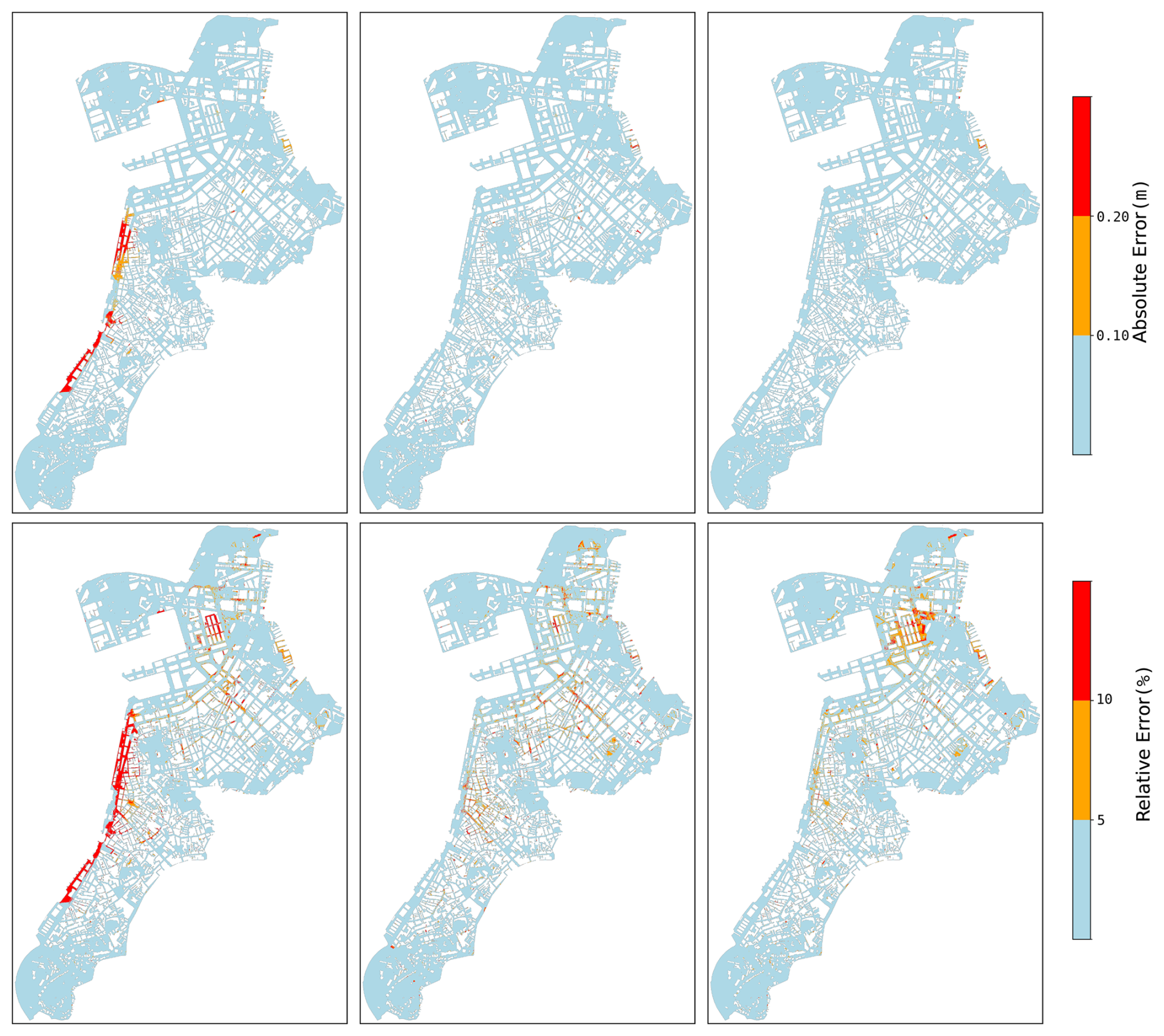
Figure 10 The absolute and relative error of maximum inundation depths. The colors represent the magnitude of the errors, with red indicating higher errors and blue indicating lower errors.

4.5 Computational efficiency

The assessment of computational efficiency between the proposed data-driven model and the physics-based model was carried out on an identical computational platform equipped with an Intel Core i9-14900K CPU (24 core, 32 threads) and an NVIDIA RTX 4090 GPU (24 GB VRAM). The model required approximately 5.2 h to complete 60 epochs, whereas the CNN-only and ConvLSTM-only baselines took 4.7 and 4.8 h. To minimize the influence of stochastic errors, the mean computation time was compared for both the data-driven model and the physics-based model in all rainfall scenarios. The physics-based model was executed utilizing the CPU, whereas the data-driven model benefited from GPU acceleration. The physics-based model required an average runtime of 16 200 s per simulation, while the pre-trained data-driven model achieved GPU-accelerated inference times of 4 s per prediction, demonstrating a 4000 × speed advantage post-training. Despite the significant initial investment associated with the high efficiency of the data-driven model, the findings suggest that it is more suitable for real-time prediction, as the training phase can be carried out during dry periods. While physics-based models are capable of obtaining computational acceleration through GPU-based parallel processing, the practical implementation of such optimizations in 1D-2D coupled hydrodynamic models continues to pose significant challenges. Present research on the utilization of GPU acceleration within the realm of physics-based models primarily concentrates on standalone 2D hydrodynamic modules, where speedups reported typically achieve an order of magnitude (e.g., 100×). This represents a substantially lower level of computational efficiency compared to the gains evidenced by data-driven methodologies.

4.6 Model robustness

The robustness of the proposed hybrid model was evaluated using k-fold event-level cross-validation. All rainfall–tide combination events were divided into ten subsets. In each iteration, nine subsets were used for training and one for validation, rotating sequentially until all subsets had served as the validation set once. Figure 11 presents the boxplots of NSE, RMSE, and MAE obtained from k-fold cross-validation across ten folds. The performance metrics exhibit consistent distributions among different folds, indicating that the model maintains stable predictive accuracy under varying training–validation splits. Specifically, NSE values remain predominantly high (generally above 0.8) with limited interquartile variability, while RMSE and MAE values stay low and comparable across folds. The median NSE values for all folds exceed 0.8, with most lying around 0.88–0.95. The first and third quartiles of NSE are typically within approximately 0.82–0.96, indicating a narrow interquartile range and consistently strong performance across samples. Correspondingly, the median RMSE values are generally below 0.15 m, with interquartile ranges mostly within about 0.07–0.18 m, while the median MAE values are mostly below 0.10 m, with interquartile ranges approximately between 0.05 and 0.15 m. Although slight differences are observed in a few folds, no systematic degradation or instability is evident. The relatively narrow interquartile ranges and similar median values across folds suggest that the model performance is not strongly dependent on a particular subset of training data. This consistency demonstrates that the proposed model generalizes well across heterogeneous samples and is not sensitive to data partitioning. Overall, the cross-validation results confirm the robustness and reliability of the model when trained on different subsets of the dataset.

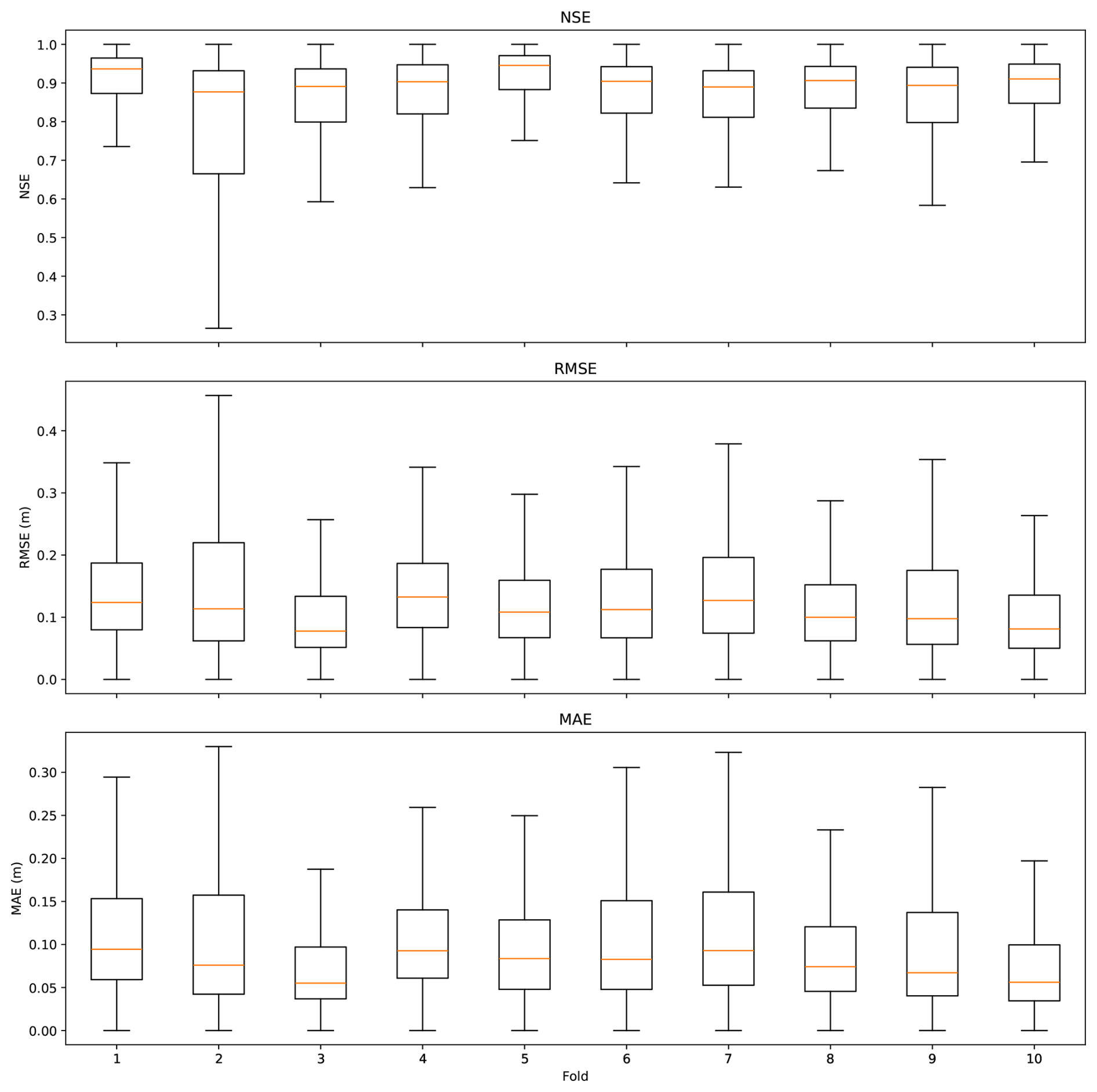
Figure 11 k-fold cross-validation results showing the distributions of NSE, RMSE, and MAE across ten folds. Boxplots display the median, interquartile range (25th–75th percentiles), and overall data spread, illustrating the variability of model performance under different training–validation splits.

4.7 Benefits of Integrating CNN and ConvLSTM Architectures

To demonstrate the effectiveness of the CNN–ConvLSTM coupled architecture proposed in this study, we compared the simulation results of the CNN-only model, the ConvLSTM-only model, and the hybrid model developed herein. Both the CNN-only and ConvLSTM-only models underwent hyperparameter optimization to determine their respective optimal network configurations. The optimized CNN-only model adopted a four-layer architecture, whereas the ConvLSTM-only model employed a two-layer architecture. The distribution of the evaluation metrics across grid cells is shown in Fig. 12.

Figure 12 compares the performance of the proposed hybrid model with the CNN-only and ConvLSTM-only models using boxplots of NSE, RMSE, and MAE. Across all three metrics, the hybrid model consistently exhibits more favorable central tendencies and comparable or smaller dispersion, indicating superior and more stable predictive performance.

For NSE, all three models achieve relatively high median values (approximately around 0.8), indicating generally good simulation skill. However, the hybrid model shows a higher lower quartile (Q1 ≈ 0.50) compared with the CNN-only (Q1 ≈ 0.33) and ConvLSTM-only (Q1 ≈ 0.35) models, suggesting that its worst-performing cases are substantially better. The upper quartiles (Q3 ≈ 0.90) are similar across models, but the narrower lower-tail spread of the hybrid model indicates improved reliability and reduced performance degradation under difficult conditions.

For RMSE, the hybrid model presents the lowest median value (≈0.12 m), compared with slightly higher medians for the CNN-only and ConvLSTM-only models (both ≈ 0.13–0.14 m). The interquartile range of the hybrid model (Q1 ≈ 0.06 m, Q3 ≈ 0.19 m) is also marginally smaller than those of the single-branch models, indicating more concentrated error distributions. Although all models show similar upper whiskers, the lower quartile improvement suggests reduced typical errors for the hybrid approach.

A similar pattern is observed for MAE. The hybrid model yields the lowest median MAE (≈0.09–0.10 m), whereas the CNN-only model exhibits a slightly higher median (≈0.10 m) and the ConvLSTM-only model lies in between. The interquartile range of the hybrid model (Q1 ≈ 0.05 m, Q3 ≈ 0.15 m) is comparable but slightly tighter than those of the other models, indicating consistently smaller absolute errors across samples.

Overall, the hybrid model demonstrates superior performance primarily through improved lower-quartile values and slightly reduced median errors across all metrics, while maintaining comparable upper-quartile performance. This indicates that integrating spatial and temporal feature extraction effectively enhances robustness and reduces the likelihood of poor predictions, leading to more reliable inundation simulations than either single-branch model alone.

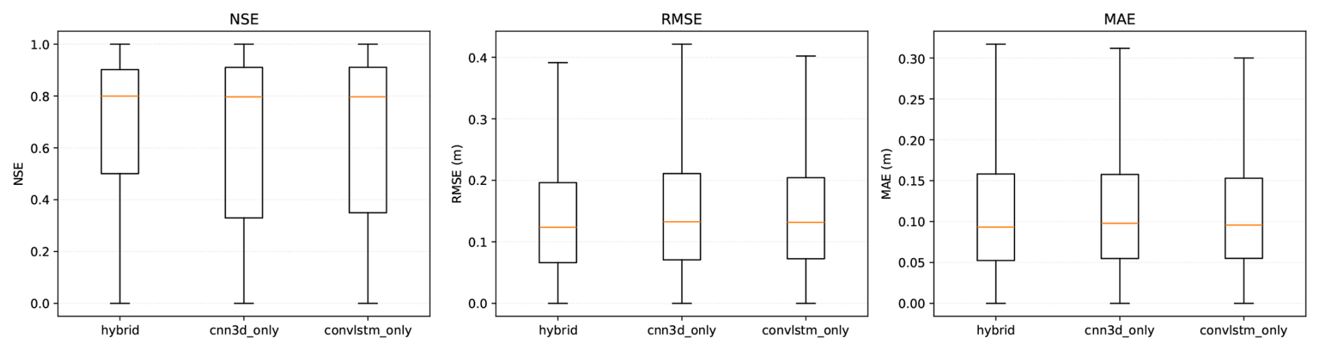
Figure 12 Distributions of NSE, RMSE, and MAE across grid cells for the hybrid, CNN-only, and ConvLSTM-only models. Boxplots display the median, interquartile range (25th–75th percentiles), and overall data spread, illustrating performance differences among the models.

5 Discussion

5.1 Model accuracy

Although the proposed data-driven model shows close agreement with the physics-based simulations at the domain scale, non-negligible discrepancies remain in areas with sharp topographic discontinuities, most notably along building peripheries. These residual errors likely arise from the combined effects of terrain representation limits, convolution-induced smoothing, the current feature-fusion design, and fundamental differences between physics-based and learning-based treatments of microscale hydraulics. The study area is densely built, with narrow gaps between adjacent structures. At the available DEM resolution, building-edge elevation transitions may be represented by only one to two grid cells. Such undersampling of high-frequency topographic variations can weaken spatial gradients in input features and reduce the model's ability to resolve discontinuities, thus concentrating errors in topographically complex edge zones (Jiang et al., 2022; Muthusamy et al., 2021; Fereshtehpour et al., 2024).

In addition, both CNN and ConvLSTM components favor smooth representations because localized convolution aggregates neighborhood information. This inductive bias can attenuate sharp transitions and may lead to over-smoothed predictions near boundaries and other high-gradient regions, consistent with prior reports on convolution-based models (Chen et al., 2019; Shi et al., 2015). Moreover, the two-branch architecture is fused through late-stage concatenation. While straightforward, late fusion may not sufficiently couple static spatial constraints (e.g., micro-topography near buildings) with the dynamic temporal evolution captured by the ConvLSTM branch, potentially weakening the influence of critical static cues during propagation (Baltrušaitis et al., 2018). Although previous studies have reported improved performance when attention-based fusion mechanisms are adopted (Vaswani et al., 2017; Lin et al., 2020), our empirical tests indicate that replacing the late-stage concatenation with an attention-based fusion strategy does not lead to further performance gains in the present model.

By contrast, physics-based models can explicitly represent building-induced flow discontinuities through numerical treatments such as building-aware terrain representation and/or localized reconstruction, which are not explicitly encoded in the current learning-based formulation. This methodological gap provides a plausible explanation for the more pronounced errors near building edges, where microscale elevation variations strongly affect flow bifurcations. Finally, the adopted loss function may place greater emphasis on spatially extensive, low-magnitude errors than on sparse but high-magnitude boundary errors, thus favoring globally averaged performance and reducing localized accuracy at building peripheries (Ronneberger et al., 2015; Kratzert et al., 2019).

Future studies may investigate the integration of building-aware terrain information, adaptive loss weighting, and enhanced fusion mechanisms to further reduce localized errors near sharp topographic discontinuities in complex urban settings.

5.2 Model interpretability

While deep learning models demonstrate considerable capabilities across various fields, they are frequently regarded as black-box models due to their complex architectures, which impede the direct interpretation of the relationships between inputs and outputs (Sayed et al., 2023; Papernot et al., 2017). Compared to physical models, their reliability in practical applications is therefore subject to more frequent scrutiny (Rudin, 2019; Yang and Chui, 2021; Nicora et al., 2022). Recent advances in explainable artificial intelligence (XAI) have sought to alleviate this limitation by developing theoretically grounded interpretability methods, such as SHAP, LIME, and related feature-attribution frameworks (Liu et al., 2024; Huang et al., 2023; Lundberg, 2017; Adadi and Berrada, 2018). However, the multidimensional nature of the inputs and outputs in this study, together with the architectural complexity of the proposed model, poses substantial challenges for global interpretability (De Mijolla et al., 2020; Saleem et al., 2022; Xu and Yang, 2025). Existing XAI techniques in hydrology and related fields remain at an early stage of development and are often limited in their ability, or computationally prohibitive, when applied to high-dimensional spatio-temporal deep learning models (Gao et al., 2025; Slater et al., 2025; Altieri et al., 2025). As a practical compromise given these constraints, SHAP analysis was conducted only at a single representative site (LHK). SHAP has emerged as one of the most widely adopted post-hoc interpretability techniques for complex neural networks. Grounded in cooperative game theory, it attributes model predictions to individual input features by estimating their marginal contributions, thereby providing a unified and theoretically consistent framework for feature attribution. Compared with gradient-based or perturbation-based approaches, SHAP satisfies desirable properties such as local accuracy and consistency, which has facilitated its application across hydrology, meteorology, and environmental sciences to investigate the relative importance of dynamic and static drivers (Savitha et al., 2025; Lundberg, 2017; Aas et al., 2021).

Although this localized analysis does not provide a full global explanation of the model behavior, it nevertheless provides useful insights into the relative importance of dynamic inputs and partially illuminates the mechanisms underlying the predicted inundation dynamics. The mean absolute SHAP values of the dynamic features are shown in Fig. 13. The results indicate that inundation depth from the preceding timestep exerts the strongest influence on the predicted inundation depth, followed by rainfall from the two preceding timesteps and tidal level from the preceding timestep. These findings are consistent with the temporal memory and boundary-driven characteristics of urban inundation processes. While the interpretability of static features was not explicitly analyzed in this study, the selection of input variables was guided by their established physical and statistical relevance to inundation dynamics, as documented in prior research (Gao et al., 2024). This design choice may help mitigate interpretability issues associated with redundant feature dimensions to some extent. Future research should prioritize the development of interpretability assessment frameworks that are better suited to multidimensional spatio-temporal models, thereby further enhancing the credibility and transparency of data-driven approaches in hydrological applications.

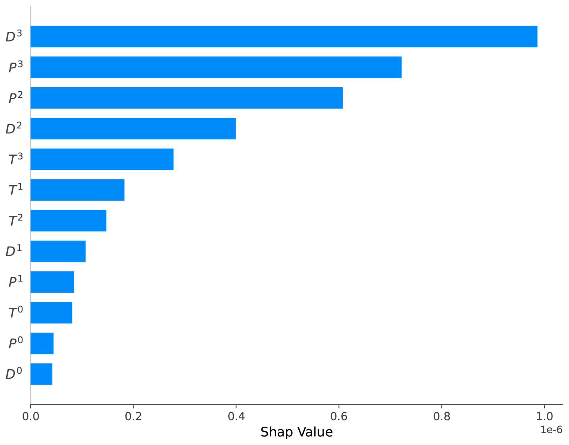
Figure 13 SHAP values of dynamic features. P^t, D^t, and T^t represent rainfall, inundation depth, and tide level at time step t, respectively. Bar lengths indicate the magnitude of each feature’s contribution to model predictions, with larger SHAP values reflecting stronger influence.

5.3 Model generalization

Recent studies have increasingly explored machine learning–based approaches for simulating urban flood dynamics, including convolutional neural networks (CNNs) (Gao et al., 2024), recurrent neural networks (RNNs) (Cao et al., 2025; Cai and Yu, 2022), ConvLSTM architectures (Liao et al., 2025; Xiao et al., 2025), and hybrid deep learning frameworks (Situ et al., 2024; Xu and Gao, 2024). These models are typically trained to predict inundation depth or flood extent using high-resolution rainfall inputs, topographic data, and, in some cases, drainage network information. A substantial proportion of existing studies focus on event-based indicators, particularly event-scale inundation depth at selected locations or aggregated spatial metrics associated with individual rainfall events. For these summary indicators, data-driven models have demonstrated relatively high predictive accuracy when calibrated and evaluated within the same urban domain, with commonly reported root mean square errors (RMSE) on the order of or below approximately 0.2 m at the event scale (Muckley and Garforth, 2021; Gao et al., 2024; Berkhahn et al., 2019).

In contrast, comparatively fewer studies attempt to explicitly simulate the full spatio-temporal evolution of urban inundation processes, including the temporal progression and spatial redistribution of floodwater during rainfall events. Recent advances have nevertheless shown that deep learning–based models can reproduce spatio-temporal inundation dynamics with satisfactory accuracy under certain conditions, demonstrating reasonable agreement with physics-based simulations or observations in terms of both inundation depth and temporal evolution, at a level comparable to that reported in this study. However, most existing studies are trained and evaluated using data from a single urban area or a fixed spatial domain, with model learning and validation conducted at the scale of the entire study region. Consequently, the reported performance primarily reflects the model’s ability to reproduce spatio-temporal dynamics within the training domain, while its capability to generalize across different spatial regions or urban settings remains less systematically assessed (Liao et al., 2025; Guo et al., 2021; Hou et al., 2021; Chen et al., 2023; Moishin et al., 2021).

A widely adopted strategy for improving the applicability of machine learning models across different urban regions is the use of transfer learning, whereby models trained in a source city are adapted to a target city through fine-tuning. While transfer learning has been shown to enhance predictive performance under cross-regional settings, it is also associated with well-recognized limitations. In particular, the fine-tuning process may lead to partial loss of previously learned knowledge, commonly referred to as catastrophic forgetting (Xu et al., 2025). Moreover, transfer learning typically relies on the availability of at least some labeled data from the target region for model adaptation, which may not always be accessible in data-scarce urban environments (Seleem et al., 2023; Zhou et al., 2023). These constraints highlight the need for alternative or complementary strategies to improve spatial generalization without strong dependence on additional regional training data.

To address the aforementioned limitations of transfer learning, the proposed approach in this study seeks to enhance spatio-temporal generalization primarily through model architecture design rather than reliance on region-specific retraining. The proposed model employs two separate encoders based on ConvLSTM and CNN architectures to process different types of input information, and is implemented within a tiling-based framework in which the study area is decomposed into multiple local spatial blocks for model training and inference. The ConvLSTM-based branch is designed to capture dynamic temporal features, such as rainfall time series, while the CNN-based branch extracts static geospatial characteristics, such as digital elevation model (DEM) data. The outputs of the two branches are then combined through a parallel concatenation operation, enabling the model to efficiently account for the joint influence of both dynamic and static factors on urban flood processes. By explicitly separating the learning of dynamic and static information streams within a unified network framework, the model is structured to capture transferable temporal patterns driven by rainfall and hydrodynamic evolution, while simultaneously encoding spatial heterogeneity associated with topography and urban form. This architectural inductive bias allows the model to learn representations that are less dependent on site-specific calibration and more robust to spatial variability.

Due to data availability constraints, the proposed model was applied and validated within a relatively limited spatial domain, which may inherently restrict a strict assessment of cross-regional generalization. However, the tiling-based design partially reflects the physical reality that individual urban drainage units often exhibit relatively localized hydrodynamic responses during flood events, which may facilitate the learning of transferable local spatial patterns and contribute to improved spatial robustness under heterogeneous conditions. Moreover, despite its limited spatial extent, the selected study area is highly urbanized and topographically heterogeneous, encompassing mountainous terrains, low-lying plains, and coastal zones. The presence of complex external boundary conditions, including tidal and marine influences, further increases the diversity of hydrodynamic regimes represented in the dataset. The adopted tile size of 200×200 m ensures that the study area yields a sufficiently large number of training and validation samples, enabling robust learning across diverse local conditions. Consequently, although the overall study area is relatively small, it can still be regarded as a meaningful and challenging testbed for evaluating the spatial generalization behavior of the proposed model. Future studies will focus on validating the proposed architecture across multiple urban regions and exploring complementary strategies, such as transfer learning or domain adaptation, to further assess and enhance its cross-regional generalization capability.

6 Conclusions

In this study, we proposed a novel deep learning model to predict the spatiotemporal distribution dynamics of urban inundation depths. The model comprises two distinct branches: a ConvLSTM-based branch and a CNN-based branch, which are amalgamated through a concatenation operation. The ConvLSTM-based branch extracts information from temporal input sequences, while the CNN-based branch captures static geospatial features. A tiling strategy was implemented during model training, partitioning the study area into spatially discrete sub-regions to serve as independent training samples, thereby enhancing generalization capability across heterogeneous terrain configurations. The proposed model was applied in a flood prone area of Macao and compared with a physics-based model. The results show that: (1) the proposed model effectively captures the dynamics of water depth in flood-prone locations, with NSE > 0.80 for the majority events, as well as RMSE and MAE values < 0.20. (2) The model demonstrates a high degree of efficiency in detecting flooding within the study area, as evidenced by a CSI value of 0.83. (3) The proposed data-driven model demonstrates robust generalization performance, with simulated inundation processes closely aligned with the results of the physics-based model in most regions (mean NSE > 0.70, RMSE < 0.10, MAE < 0.10). Notable discrepancies persist only in localized zones of abrupt terrain variations, particularly near building edges. Overall, the results indicate that the proposed framework effectively simulates urban inundation dynamics. The modeling strategy, which integrates spatiotemporal feature learning with a tiling-based training scheme, provides a practical solution for large-scale urban flood analysis under heterogeneous surface conditions.