Prediction of basin-scale river channel migration based on landscape evolution numerical simulation

The basin-scale river channel migration, driven by multiple factors such as hydrometeorological conditions, tectonic movements, and human activities, exerts a profound influence on regional morphological features, water resource, and ecosystem over long-term evolution. Conventional river dynamics approaches struggle to quantitatively characterize basin-scale channel migration due to difficulties in incorporating factors like basin hydrological processes and tectonic activities. This study proposed a novel technique for the numerical simulation of river channel migration, integrating a fully coupled multi-processes landscape evolution model (e.g., hydrological, geomorphic and tectonic processes) with channel extraction. Furthermore, to address model parameter uncertainty, a Markov chain Monte Carlo (MCMC) method with a modified likelihood function is used for parameter uncertainty quantification. Simultaneously, a computationally efficient Long Short-Term Memory (LSTM)-based surrogate model for channel migration is developed to overcome the computational bottleneck in uncertainty analysis. Applied to the Kumalake River Basin within China's Tarim Basin, the study employs the Landscape Evolution-Penn State Integrated Hydrologic Model (LE-PIHM) to construct the landscape evolution model. Combined with channel extraction, it simulates historical (2000–2021) and future (2021–2100) landscape evolution and channel migration processes. Results demonstrated that the developed river channel migration model, aided by parameter uncertainty analysis, reliably captures the dynamics of channel migration in the study area during 2000–2021. Additionally, the LSTM-based surrogate model achieves high accuracy, effectively resolving computational challenges in parameter uncertainty analysis. Predictions under different climate scenarios reveal significant variations in future channel evolution, indicating that climate change will profoundly reshape basin geomorphic features and river patterns.

1 Introduction

Basin-scale river channel migration is the result of interactions among multiple spheres within the complex earth system, influenced by various factors including meteorological, hydrological, and geological conditions (Li et al., 2023; Desormeaux et al., 2022). Over long temporal and basin scales, river channel migration regulates the spatial configuration of river networks, exerting significant impacts on regional water resources, ecological environments, and the development of civilizations. For instance, the substantial downstream migration of the Euphrates River between approximately 2112–2004 BCE contributed to the collapse of the Sumerian civilization (Hritz, 2010). The diversion of the lower Tarim River in 630 CE led to the disappearance of the ancient Loulan Kingdom (Yu et al., 2016; Shao et al., 2022). Quantitative research on river channel migration at the basin scale is crucial; it can not only inform projections of water resource distribution under climate change scenarios but also facilitate the reconstruction of linkages among channel evolution, fluvial ecosystems, and the trajectories of human civilizations (Hickin 1983; Zhou et al., 2022; Zhen et al., 2025).

River channel migration in the basin scale involves multiple coupled processes including surface water and groundwater water, weathering and erosion, and tectonic uplift. In particular, groundwater flow under real-world complex conditions may exhibit multi-scale heterogeneity (Lu et al., 2023). Together, these processes operate across broad spatiotemporal scales, exhibit complex mechanistic interactions, and are highly susceptible to anthropogenic disturbance. Numerical modeling therefore serves as the principal approach for quantitatively characterizing these dynamics. Among various modeling strategies, river channel migration models grounded in fluvial dynamics have been widely used. For example, Ikeda et al. (1981) developed a single meander segment model by coupling flow fields with erosion rates. Morón et al. (2017) employed Delft3D (Lesser et al., 2004) to simulate the evolution of channel segments in the Nile River, Columbia River, Congo River and Negro River. Hsu and Hsu (2022) utilized Nays2DH (Ali et al., 2017) to simulate braided river morphology in the lower Dajia River, and identified that channel width as a primary factor governing migration direction. However, these methods generally focus on partial river channel domains (e.g., meander reaches) and fail to incorporate hydrologic processes and tectonic activities at the basin scale, thus limiting their applicability to river channel migration over engineering timescales and channel segment scales.

As a typical geomorphic unit, river channels are fundamentally governed by landscape evolution processes (Lisenby et al., 2020). Landscape evolution models (LEMs) are numerical tools designed to quantify elevation changes across watersheds over geological timescales, incorporating hydrologic processes and tectonic uplift (Bishop, 2007; Tucker and Hancock, 2010; Hou et al., 2025). By integrating LEMs with river channel extraction techniques, it becomes feasible to simulate long-term, basin-scale channel migration. Commonly used LEMs include CASCADE (Braun and Sambridge, 1997), CHILD (Tucker et al., 2001), CAESAR-Lisflood (Coulthard et al., 2013), DAC (Goren et al., 2014; Yang et al., 2015), Landlab (Barnhart et al., 2020; Litwin et al., 2024), all of which have been widely used for simulating landscape evolution. Nevertheless, these models often simplify or neglect groundwater dynamics and lateral erosion processes (Whipple et al., 2017), making it difficult to accurately capture these crucial hydrological and geomorphic processes in large-scale, long-term watershed landscape evolution simulations.

Zhang et al. (2016) developed LE-PIHM by coupling surface-subsurface hydrologic processes with slope and channel sediment transport, while accounting for bedrock weathering and tectonic uplift, based on the PIHM framework (Qu and Duffy, 2007). LE-PIHM is particularly suited for quantifying landscape evolution processes over long durations and basin extents. Nevertheless, current studies rarely integrate multiple processes for real basin-scale simulations of coupled landscape evolution and river channel migration. Meanwhile, LEMs contain a large number of parameters to be identified, the non-negligible parameters uncertainty can lead to unreliable simulations of landscape evolution and river channel migration, which has not been adequately addressed in current researches (Temme et al., 2009; Neuendorf et al., 2018; Xu et al., 2024). To quantify river channel migration at the basin scale under the coupled effects of multiple processes, the LE-PIHM was used to establish a landscape evolution model in this study, and the distribution of river channels was identified using a river channel extraction technique. In addition, Long Short-Term Memory (LSTM) surrogate modeling and Bayesian uncertainty analysis were employed to quantify parameter uncertainty in the LEMs.

This study selects the Kumalake River Basin within China's Xinjiang Tarim Basin as the research area. This basin features diverse geomorphic types and complex climatic conditions, and has experienced significant river channel migration in recent decades (Wang et al., 2024), making it an ideal site for conducting basin-scale simulations of terrain evolution and river channel dynamics. Based on the identified model parameters distribution of LE-PIHM, the river channel migration process in the study area over the past two decades was quantitatively reconstructed. Finally, this study conducted future scenario simulations of landscape evolution and river channel migration under projected climate change through the end of the 21st century.

The structure of this paper is as follows: Section 2 outlines the methodology and overall workflow; Sect. 3 introduces the construction of the basin-scale river channel migration model and the development of an LSTM-based surrogate model for uncertainty analysis; Sect. 4 presents the results and discussion; and Sect. 5 provides concluding remarks and summarizes the key findings.

2 Methodology

2.1 Framework of basin-scale river channel migration prediction

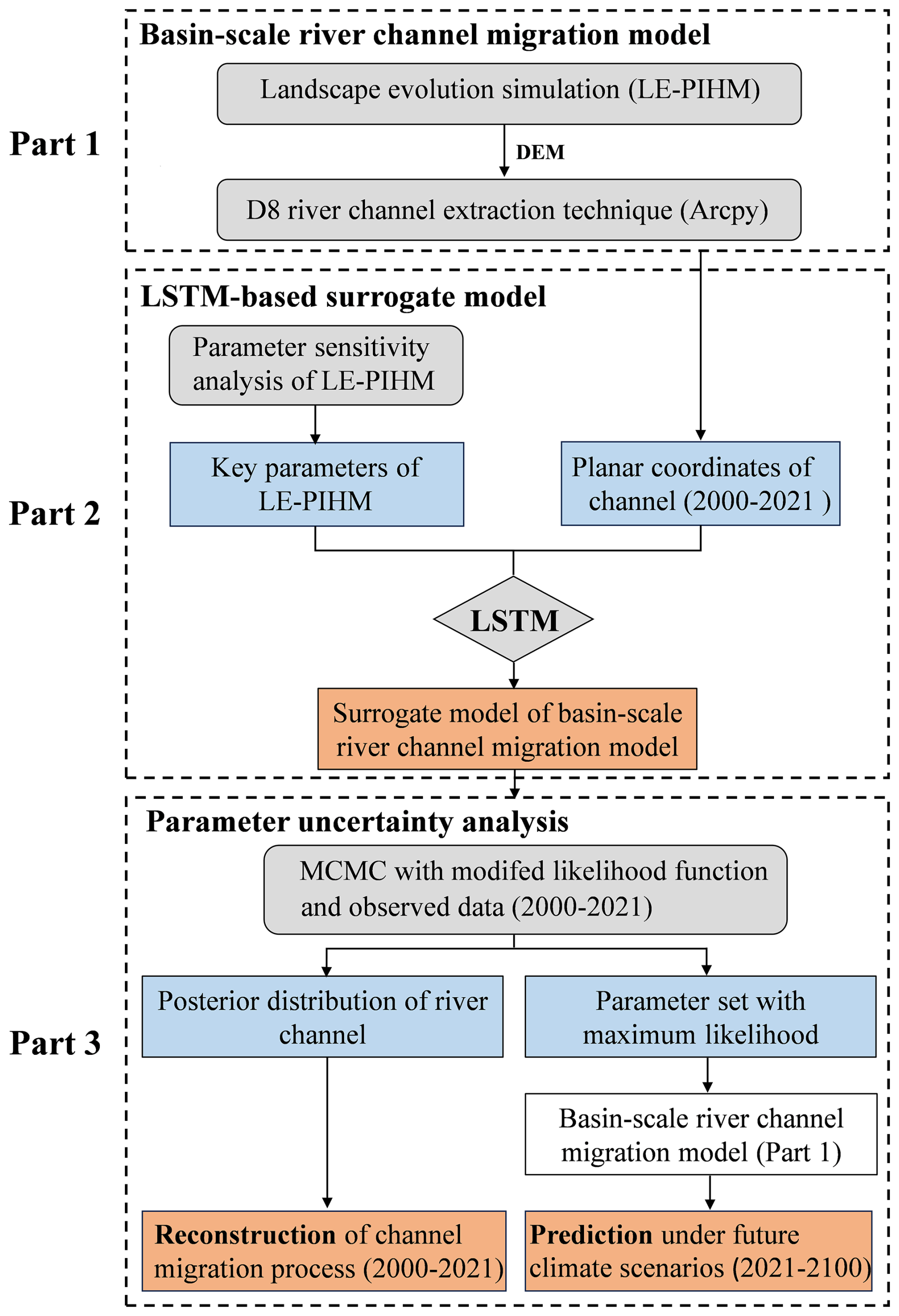
The framework of predicting basin-scale river channel migration in this paper consists of three parts (Fig. 1).

Part 1:

Establishment of the basin-scale river channel migration model. The basin-scale river channel migration model is implemented in two steps. First, landscape evolution is simulated using LE-PIHM to obtain the elevation distribution of the study area. Subsequently, the DEM is processed using the D8 algorithm to extract the spatial distribution of river channel.

Part 2:

Development of a LSTM-based surrogate model for efficient parameter uncertainty analysis. To improve the efficiency of parameter identification, a surrogate model corresponding to the original river channel migration model (Part 1) is developed for the reconstruction period (2000–2021). Parameter sensitivity analysis is first conducted to identify the key landscape evolution parameters of LE-PIHM. Then, 3000 parameter sets are sampled and input into the basin-scale river channel migration model (Part 1) to generate the associated planar channel coordinates, which serve as the training datasets. The LSTM is trained using these data to construct a surrogate model of basin-scale river channel migration, substantially reducing the computational burden of parameter uncertainty analysis.

Part 3:

Parameter uncertainty analysis and the prediction of channel migration. Based on the LSTM-based surrogate model (Part 2), parameter uncertainty analysis is conducted using a modified-likelihood Markov chain Monte Carlo (MCMC) approach constrained by observed river channel data from 2000–2021. The resulting posterior distribution of river channel enable the reconstruction of channel migration processes over 2000–2021. The maximum-likelihood posterior parameter set is then selected, and the original river channel migration model (Part 1) is executed under future climate scenarios to predict channel migration from 2021–2100.

Figure 1 Technical roadmap of basin-scale river channel migration prediction.

2.2 Basin-scale river channel migration model

2.2.1 Landscape evolution simulation

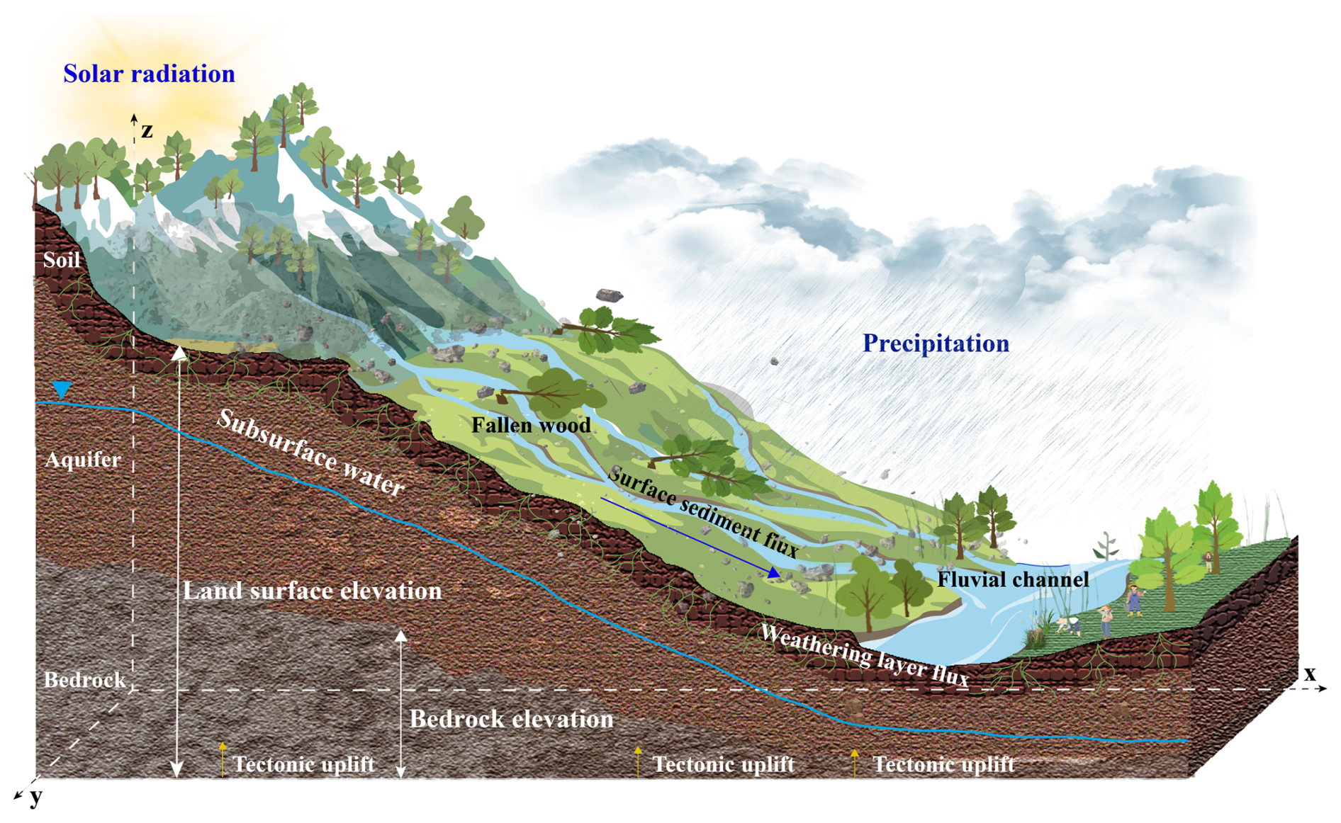
The Landscape Evolution-Penn State Integrated Hydrologic Model (LE-PIHM) was used to simulate the landscape evolution processes. LE-PIHM couples the processes of surface water and groundwater, snow accumulation and melt, hillslope and river channel sediment transport, weathering and erosion, as well as tectonic uplift (Fig. 2). It is a basin-scale fully coupled hydrologic-process-based landscape evolution model (Zhang et al., 2016). The hydrologic and geomorphic modules are tightly coupled within the same control volume through mass conservation and flux closure, and the state variables are updated synchronously at each time step. For each grid element (a Triangulated Irregular Network, TIN), the model simultaneously tracks seven state variables: canopy water storage, snowpack, surface-water depth, vadose-zone water storage, saturated-zone groundwater table, land-surface elevation, and bedrock-interface elevation. These state variables are assembled into a unified global system of ordinary differential equations and are solved concurrently. Within each TIN control volume, multiple fluxes including infiltration, recharge, overland flow, groundwater flow, and sediment/weathering/uplift fluxes coexist and are transported in a coupled manner across the entire TIN mesh domain.

Figure 2 Schematic diagram of the Landscape evolution process.

The model simulates surface elevation change based on the principle of mass continuity. According to the law of mass conservation, the geomorphic process equation can be expressed as the temporal variation of the mass of the regolith and bedrock.

$$\begin{array}{}\text{(1)}& \begin{array}{rl}{\displaystyle }& {\displaystyle \frac{\partial \left({\mathit{\sigma }}_{\text{re}}h\mathrm{d}x\mathrm{d}y\right)}{\partial t}}+{\displaystyle \frac{\partial \left({\mathit{\sigma }}_{\text{ro}}e\mathrm{d}x\mathrm{d}y\right)}{\partial t}}=\\ {\displaystyle }& {\displaystyle }{\mathit{\sigma }}_{\text{re}}{q}_{\mathrm{c}}\mathrm{d}y-\left[{\mathit{\sigma }}_{\text{re}}{q}_{\mathrm{c}}\mathrm{d}y+{\displaystyle \frac{\partial \left({\mathit{\sigma }}_{\text{re}}{q}_{\mathrm{c}}\mathrm{d}y\right)}{\partial x}}\mathrm{d}x\right]\\ {\displaystyle }& {\displaystyle }+{\mathit{\sigma }}_{\text{re}}{q}_{\mathrm{c}}\mathrm{d}x-\left[{\mathit{\sigma }}_{\text{re}}{q}_{\mathrm{c}}\mathrm{d}x+{\displaystyle \frac{\partial \left({\mathit{\sigma }}_{\text{re}}{q}_{\mathrm{c}}\mathrm{d}y\right)}{\partial y}}\mathrm{d}y\right]\\ {\displaystyle }& {\displaystyle }+{\mathit{\sigma }}_{\text{re}}{q}_{\mathrm{s}}\mathrm{d}y-\left[{\mathit{\sigma }}_{\text{re}}{q}_{\mathrm{s}}\mathrm{d}x+{\displaystyle \frac{\partial \left({\mathit{\sigma }}_{\text{re}}{q}_{\mathrm{s}}\mathrm{d}y\right)}{\partial y}}\mathrm{d}x\right]\\ {\displaystyle }& {\displaystyle }+{\mathit{\sigma }}_{\text{re}}{q}_{\mathrm{s}}\mathrm{d}x-\left[{\mathit{\sigma }}_{\text{re}}{q}_{\mathrm{s}}\mathrm{d}x+{\displaystyle \frac{\partial \left({\mathit{\sigma }}_{\text{re}}{q}_{\mathrm{s}}\mathrm{d}y\right)}{\partial y}}\mathrm{d}y\right]\\ {\displaystyle }& {\displaystyle }\times {\mathit{\sigma }}_{\text{ro}}U\mathrm{d}x\mathrm{d}y\end{array}\end{array}$$

where σ_re is the bulk density of regolith (kg m⁻³);σ_ro is the bulk density of bedrock (kg m⁻³); h is the regolith thickness (m); e is the elevation of the bedrock surface (m); The regolith thickness h is defined as the difference between the ground surface elevation z and the bedrock elevation e; q_c is the lateral volumetric flux of regolith (m² yr⁻¹), driven by processes such as soil creep; q_s is the surface sediment flux by overland flow (m² yr⁻¹); U is the tectonic uplift rate (m yr⁻¹).

The governing equations for hydrologic processes describe the water flux dynamics from the vegetation canopy to the regolith layer. These processes can be represented as follows:

$$\begin{array}{}\text{(2)}& \left\{\begin{array}{ll}& {\displaystyle \frac{\partial {\mathit{\psi }}_{\text{canopy}}}{\partial t}}=\text{vFrac}(\mathrm{1}-f_{\mathrm{S}})p-E_{\mathrm{c}}-\text{TF}\\ & {\displaystyle \frac{\partial {\mathit{\psi }}_{\text{snow}}}{\partial t}}=f_{\mathrm{S}}p-\text{SM}\\ & {\displaystyle \frac{\partial {\mathit{\psi }}_{\text{surf}}}{\partial t}}=\mathrm{\nabla }{q}_{\text{sw}}+p_{\text{net}}-I-E_{\mathrm{s}}\\ & {\displaystyle \frac{\partial {\mathit{\psi }}_{\text{unsat}}}{\partial t}}=I-R-E_{\mathrm{g}}-E_{\text{gt}}\\ & {\displaystyle \frac{\partial {\mathit{\psi }}_{\text{sat}}}{\partial t}}=\mathrm{\nabla }{q}_{\text{gw}}+R-E_{\text{sat}}-E_{\text{tsat}}\end{array}\right.\end{array}$$

where: Ψ_canopy is the canopy water storage (m); Ψ_snow is the snow depth (m); Ψ_surf is the surface water depth (m); Ψ_unsat is the water storage in the unsaturated zone (m); Ψ_sat is the groundwater (saturated zone) storage (m); vFrac is the fraction of vegetation coverage; f_s is the fraction of precipitation falling as snow; P is the precipitation rate (m d⁻¹); E_c and E_s are the evaporation rates from the canopy and surface water, respectively (m d⁻¹); TF is the throughfall rate from canopy to ground (m d⁻¹); SM is the snowmelt rate (m d⁻¹); p_net is the net precipitation reaching the ground surface (m d⁻¹); I is the infiltration rate (m d⁻¹); E_g and E_sat are the evaporation rates from the unsaturated and saturated zones, respectively (m d⁻¹); E_gt and E_tsat are the transpiration rates from the unsaturated and saturated zones, respectively (m d⁻¹); q_sw is the unit-width overland flow rate (m² d⁻¹); q_gw is the unit-width groundwater (lateral) flow rate (m² d⁻¹).

The values of q_sw and q_gw are determined by the Manning equation and Darcy's law, respectively, as follows:

$$\begin{array}{}\text{(3)}& {\displaystyle }{q}_{\text{sw}}=& {\displaystyle \frac{{\mathit{\psi }}_{\text{surf}}^{\mathrm{5}/\mathrm{3}}}{n_{\mathrm{s}}}}\left(\mathrm{\nabla }\right({\mathit{\psi }}_{\text{surf}}+z\left){)}^{\mathrm{1}/\mathrm{2}}\right)\text{(4)}& {\displaystyle }{q}_{\text{gw}}=& {\displaystyle }{\mathit{\psi }}_{\text{sat}}{k}_{\text{sat}}\mathrm{\nabla }({\mathit{\psi }}_{\text{sat}}+e)\end{array}$$

where n_s is the Manning's roughness coefficient; k_sat is the horizontal hydraulic conductivity of the aquifer (m d⁻¹). For detailed formulas and variable descriptions, please refer to Qu and Duffy (2007).

In summary, topography elevation and bedrock elevation determine hydraulic slopes and head gradients, whereas hydrologic states (e.g., surface-water depth and groundwater level) govern shear stress and sediment-transport capacity. Sediment fluxes (q_s), hillslope fluxes (q_c), and uplift terms are solved in a coupled manner to update elevations, which in turn modify hydraulic gradients and flow-routing patterns. This two-way feedback implies that the evolving landscape constrains river dynamics, and river processes reshape the landscape, thereby forming a self-consistent loop of hydro-geomorphic co-evolution. Collectively, The governing equations (1–4) couple hydrological processes, hillslope and channel sediment transport processes, and tectonic movements to form a state-of-the-art hydro-geomorphic model for simulating landscape evolution.

2.2.2 D8 algorithm river channel extraction technique

The river channel extraction in basin-scale is implemented through a topography-based extraction technique. This technique is based on the principle of maximum gradient and identifies river channels within the watershed using surface elevation data. Specifically, the landscape evolution simulation provides the surface elevation distribution of the study area, from which a digital elevation model (DEM) is constructed. The DEM is first filled to remove depressions, followed by spatial analysis to determine surface flow direction and compute flow accumulation. River channel distribution is then extracted based on the accumulated flow.

The standard D8 algorithm, known for its simplicity and practicality, is currently the most widely used and reliable method for determining water flowpaths from DEM (O'Callaghan and Mark, 1984; Tarboton, 1997). The ArcPy scripting in ArcGIS, which implements the standard D8 algorithm (Esri, 2022), will be used in this study to extract watershed river channels through the ArcGIS hydrological analysis platform.

2.2.3 Long Short-Term Memory algorithm

Long Short-Term Memory (LSTM) is a specialized type of Recurrent Neural Network (RNN), originally proposed by Hochreiter and Schmidhuber (1997) and later extended and popularized by Graves and Schmidhuber (2005). Traditional RNNs often suffer from the vanishing or exploding gradient problem when processing long sequential data, making it difficult to capture long-term dependencies effectively. LSTM addresses this issue by introducing gated mechanisms namely the forget gate, input gate, and output gate, which dynamically regulate the flow of information. These gates allow the network to selectively store, update, and output information within memory cells, thereby effectively addressing the gradient instability problem in long-sequence modeling.

To address the computational burden caused by repeated model evaluations during the parameter uncertainty analysis of the basin-scale river channel migration model, this study constructs a surrogate model using an LSTM network. Specifically, the LSTM algorithm is employed to build the nonlinear response relationship between the key parameters of LE-PIHM and the spatial distribution of river channels (i.e., planar coordinates of reaches) within the study area.

2.3 Bayesian uncertainty analysis

2.3.1 Markov chain Monte Carlo simulation

Markov chain Monte Carlo (MCMC) is a statistical simulation technique based on Bayesian theory. Its core idea is to construct a Markov chain that iteratively explores the parameter probability space to generate samples from the target posterior distribution. As the chain evolves, its stationary distribution converges to the posterior distribution of the parameters of interest (Vrugt et al., 2009).

MCMC integrates observational data through Bayes' theorem, enabling parameter samples to progressively converge from the prior distribution p(θ) to the posterior distribution p(θ|D).

$$\begin{array}{}\text{(5)}& p\left(\mathit{\theta }\mathrm{|}D\right)={\displaystyle \frac{L\left(\mathit{\theta }\mathrm{|}D\right)p\left(\mathit{\theta }\right)}{\int L\left(\mathit{\theta }\mathrm{|}D\right)P\left(\mathit{\theta }\right)d\left(\mathit{\theta }\right)}}\end{array}$$

where L(θ|D) represents the likelihood function of a parameter sample θ, D represents the observed data. The likelihood function L is typically defined as a Gaussian likelihood function:

$$\begin{array}{}\text{(6)}& \begin{array}{rl}{\displaystyle }L\left({\mathit{\theta }}^i\mathrm{|}D\right)=& {\displaystyle \frac{\mathrm{1}}{\mathrm{2}{\mathit{\pi }}^{n/\mathrm{2}}\mathrm{|}\sum {\mathrm{|}}^{\mathrm{1}/\mathrm{2}}}}\\ {\displaystyle }& {\displaystyle }\times \exp \left[-{\displaystyle \frac{[D-f({\mathit{\theta }}^i\left){]}^T{\sum }^{-\mathrm{1}}\right[D-f\left({\mathit{\theta }}^i\right)]}{\mathrm{2}}}\right]\end{array}\end{array}$$

where n is the number of observed data points, f(θⁱ) denotes the hydrologic model simulation result given the parameter θⁱ, and Σ is the covariance matrix of the simulation residuals.

2.3.2 Hausdorff distance and the modified likelihood function

The Hausdorff distance is employed as a metric to quantify the discrepancy between the simulated and the observed river channels. The Hausdorff distance is a well-established measure of curve-to-curve spatial similarity and has been widely applied in studies of river-morphology matching, path comparison, and geomorphic feature shape analysis (Lei and Lei, 2022; Bogoya et al., 2019; Ranacher and Tzavella, 2014). The Hausdorff distance summarizes distances across all discretized points along the entire channel, thereby accounting for both the overall displacement and differences in channel curvature and planform geometry.

The core concept of the Hausdorff distance is to treat two curves as two sets of discrete points (Fig. 3). Suppose we have two point-sets, $A=\mathit{\{}{a}_{\mathrm{1}},\mathrm{\dots },a_p\mathit{\}}$, $B=\mathit{\{}{b}_{\mathrm{1}},\mathrm{\dots },b_{\mathrm{q}}\mathit{\}}$, p and q represent the number of points in sets A and B, respectively, the bidirectional Hausdorff distance HD(A,B) between sets A and B is defined as:

$$\begin{array}{}\text{(7)}& \text{HD}(A,B)=\text{Max}\left[h\right(A,B),h(B,A\left)\right]\end{array}$$

where h(A,B) and h(B,A) represent the one-sided Hausdorff distances. Specifically, h(A,B) denotes the set of minimum distances from each point in set A to the nearest point in set B, $h(A,B)=h(a_{\mathrm{1}\min },a_{\mathrm{2}\min },\mathrm{\dots },a_{\text{pmin}})$, where a_1 min is the minimum distance from point a₁ to the points in set B. Similarly, $h(B,A)=h(b_{\mathrm{1}\min },b_{\mathrm{2}\min },\mathrm{\dots },b_{\text{pmin}})$ which denotes the set of minimum distances from each point in B to the nearest point in A.

Figure 3 Conceptual schematic diagram of Hausdorff distance.

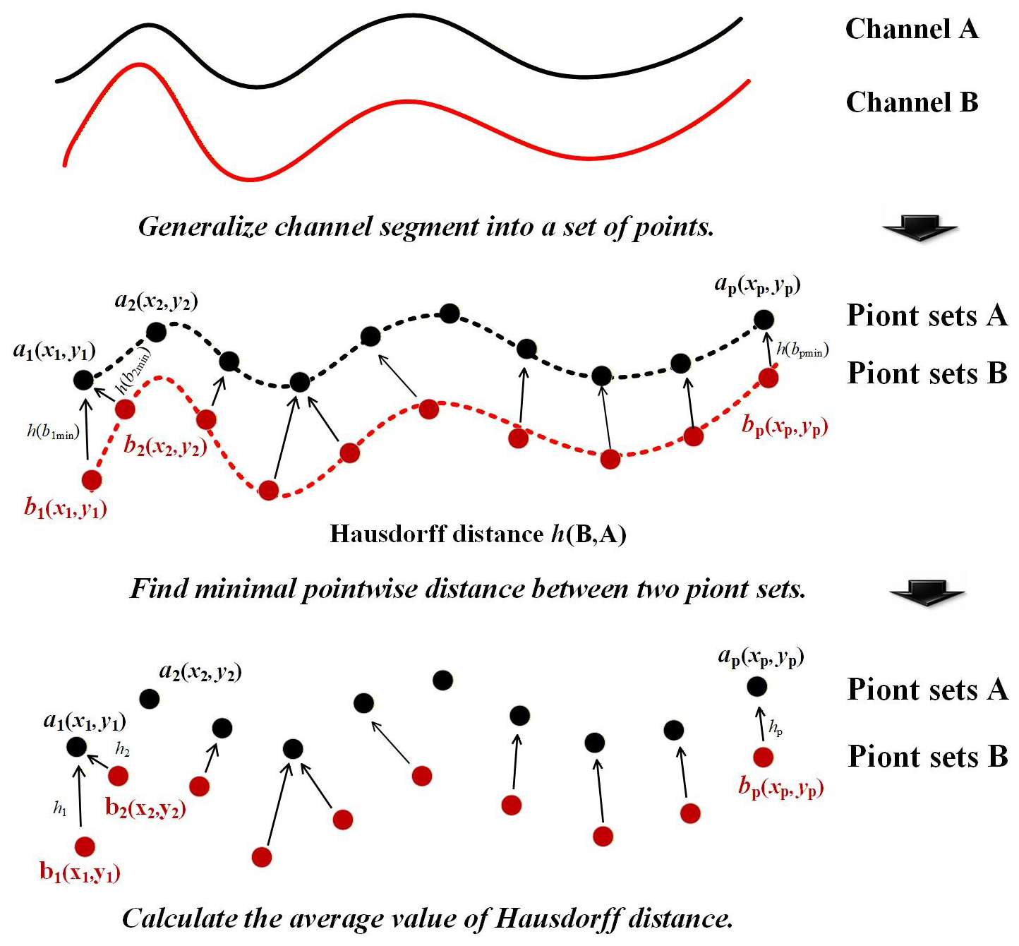
In this study, we modified Eq. (7) by replacing the maximum operation in the one-sided distance with the mean of the minimum distances, and set p equal to q. This modification better captures the overall spatial discrepancy between two river channel curves and is referred to as the average Hausdorff distance (H). A smaller value of H indicates that the simulated river channel more closely matches the observed channel.

$$\begin{array}{}\text{(8)}& H={\displaystyle \frac{\mathrm{1}}{\mathrm{2}p}}\sum _{i=\mathrm{1}}^p\left[h\right(A,B)+h(B,A\left)\right]\end{array}$$

In the uncertainty analysis of river channel migration simulation, the likelihood function quantifies the degree of fit between the simulated and observed river channels. To enable the parameter uncertainty quantification through MCMC, the original likelihood function (i.e., Eq. 6) is revised by treating the average Hausdorff distance (H) as the simulation target. The observed value of H (denoted as H_obs) is set to 0, this indicates the H between the real river channel and itself. Meanwhile, the Σ in Eq. (6) collapses to a single variance term, and the residuals in likelihood function can be expressed as:

$$\begin{array}{}\text{(9)}& D-f\left({\mathit{\theta }}^i\right)=H-H_{\text{obs}}=H-\mathrm{0}=H\end{array}$$

The observation error of H_obs is treated as a random error variable that follows a zero-mean, independent and identically distributed gaussian error model, i.e., N(0,σ²). Combining Eq. (6) with Eq. (9) and taking the natural logarithm, a modified likelihood function designed for quantifying river channel simulation is obtained:

$$\begin{array}{}\text{(10)}& \ln L=-{\displaystyle \frac{\mathrm{1}}{\mathrm{2}}}\left[{\displaystyle \frac{H^{\mathrm{2}}}{{\mathit{\sigma }}^{\mathrm{2}}}}+\ln \left(\mathrm{2}\mathit{\pi }{\mathit{\sigma }}^{\mathrm{2}}\right)\right]\end{array}$$

In other words, this modified form of the likelihood function (Eq. 10) is used in the MCMC-based uncertainty analysis of river channel model parameters.

3 Construction of the river channel migration model

3.1 Study area

The Kumalake River Basin is located in the northwestern corner of the Tarim Basin in Xinjiang, China, covering an area of about 3500 square kilometers. The basin is bordered by the towering Tianshan mountains to the north, the flat Aksu Plain to the south, and the Toxkan River Basin to the west. The landscape exhibits a distinct elevation gradient sloping from north to south, with a complex geomorphic setting comprising mountainous hillslopes, valley plains, and fluvial terraces (Fig. 4). The Kumalake River, approximately 89.34 km in length, is the largest tributary of the Aksu River. It flows from the northwest to the southeast across the study area and exits at the southeastern edge of the basin, where it joins the Tuoshigan River. The combined flow continues into the Aksu River and eventually discharges into the main stem of the Tarim River (Tang et al., 2007).

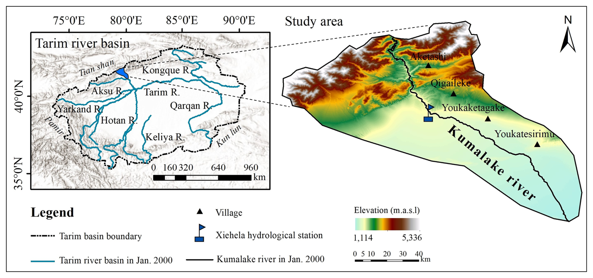
Figure 4 Schematic diagram of the watershed in the study area. Basemap: Esri World Hillshade | Powered by Esri.

The Kumalake River has experienced pronounced channel migration during the last two decades. This study selects the Kumalake River Basin as the case study area, with a focus on simulating river channel migration over the period from 2000–2021. The simulation is conducted within the landscape evolution modeling framework, and a parameter uncertainty analysis is performed to improve the reliability of the model outputs.

3.2 Model input data

In this study, LE-PIHM combined with a river channel extraction technique is employed to simulate the spatial distribution of river channels. Notably, four categories of physical properties within the study area, i.e., soil, aquifer, bedrock, and land cover, exhibit significant spatial heterogeneity (see Table 1 and Fig. 5). The driving force data in LE-PIHM primarily include leaf area index, precipitation rate, air temperature, downward shortwave radiation, snowmelt rate, wind speed, and relative humidity (Table 1)

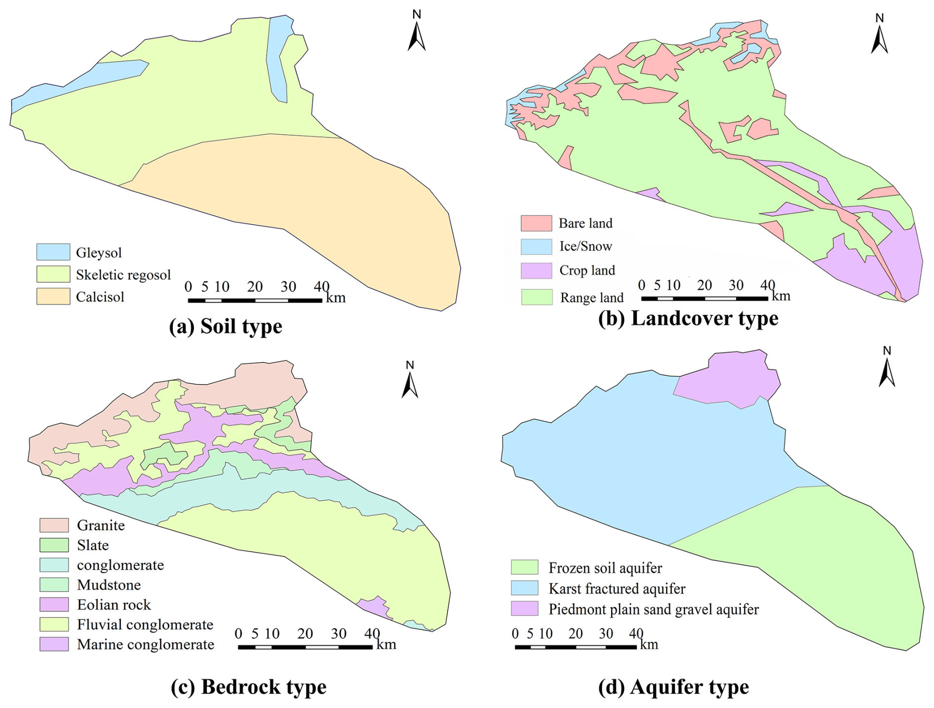
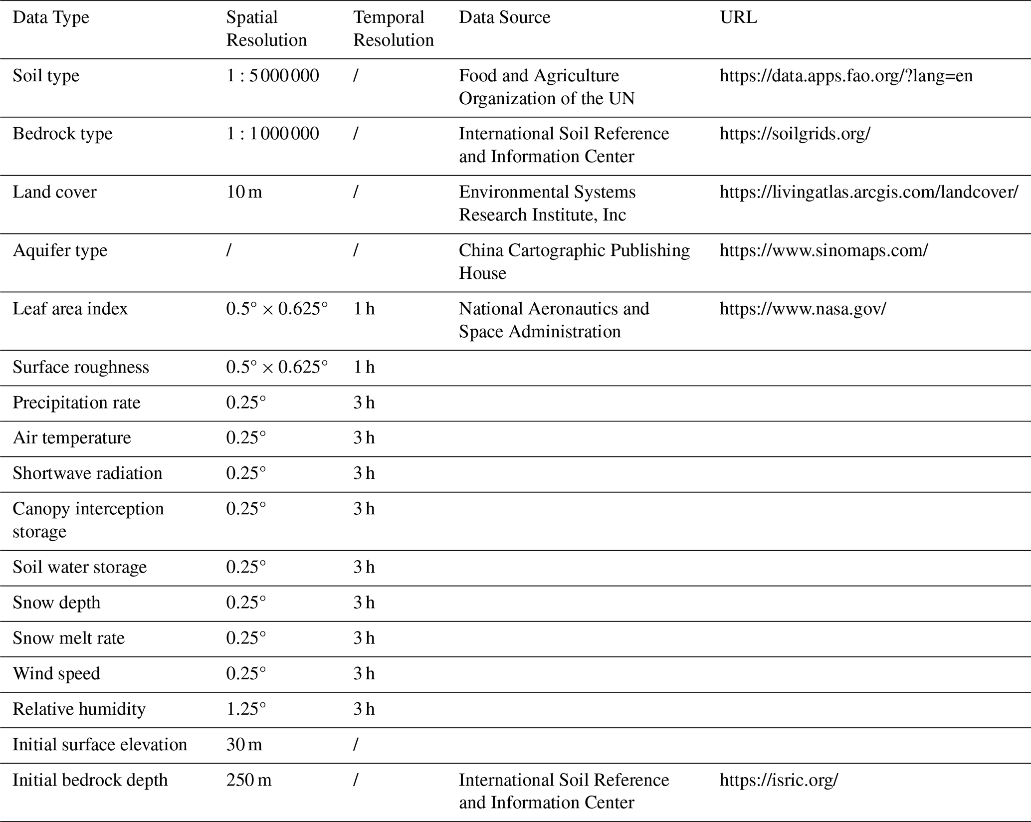
Figure 5 Zonation of average tectonic uplift rates in the study area from 2000–2021.

Table 1 Types and sources of input data for the landscape evolution model.

All links in the table were last accessed on 2 December 2025.

As an essential driving factor in landscape evolution, the rock uplift rate data were derived from the vertical crustal velocity field of China (Wang and Shen, 2020; Zubovich et al., 2016), with the Chinese GNSS velocity field taken from Wang and Shen (2020; https://doi.org/10.7910/DVN/C1WE3N, Shen, 2019) and the Pamir–Tien Shan GNSS velocities from Zubovich et al. (2016; https://doi.org/10.1002/2015TC004055). The spatial distribution of the average rock uplift rate in the study area from 2000–2021 was obtained through kriging interpolation (Fig. 6).

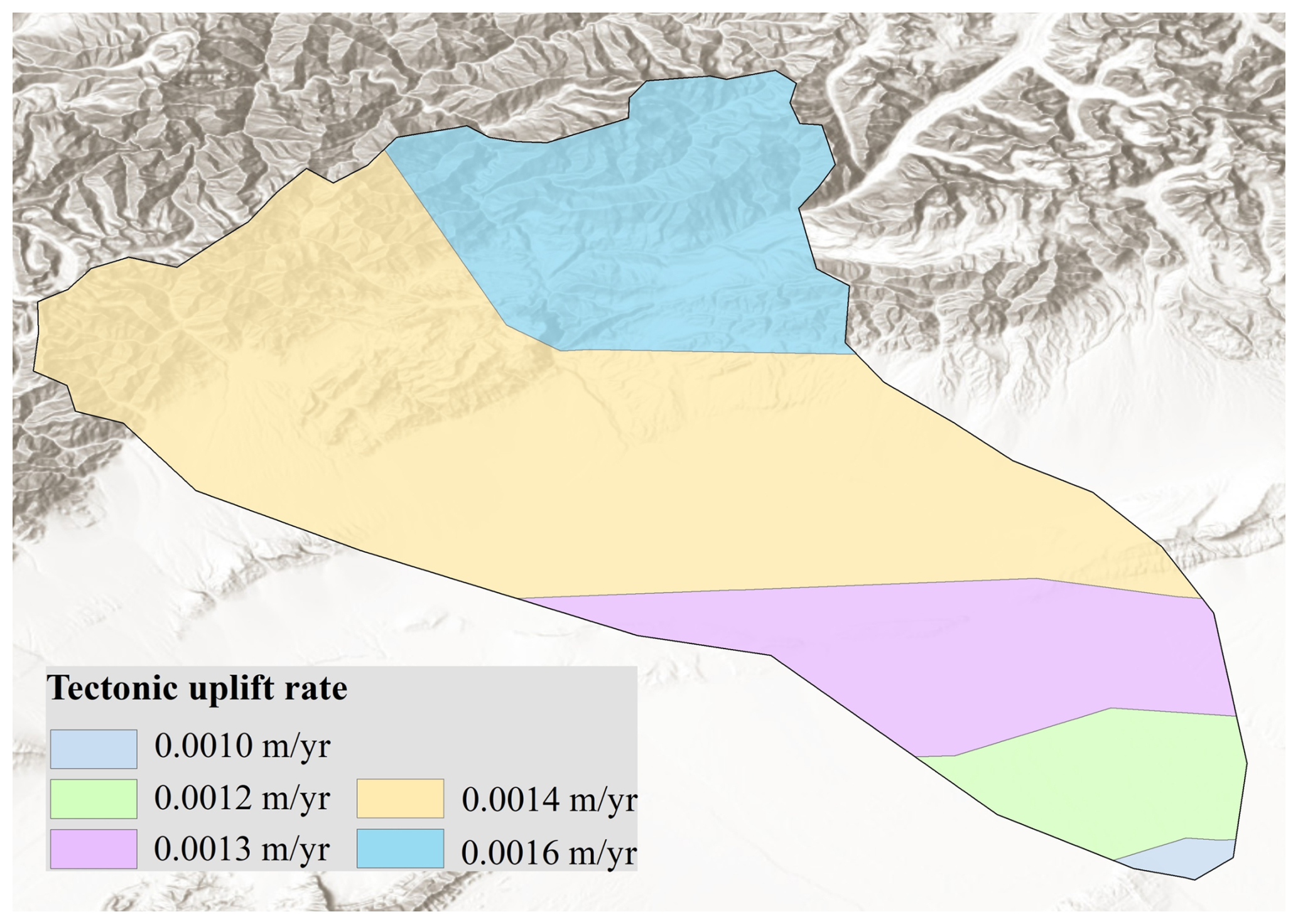
Figure 6 Zonation of average tectonic uplift rates in the study area from 2000–2021. Basemap: Esri World Hillshade | Powered by Esri.

3.3 Observed river channel planform data

Observed river channel planform data for December 2007, February 2014, and December 2021 were obtained using the Google Earth Pro image platform (see Fig. 7). Among these, the spatial distribution of river channels from December 2007 and February 2014 were used to identify the posterior distribution of model parameters (i.e., key parameters of LE-PIHM), while the December 2021 data were employed to validate the river channel migration results.

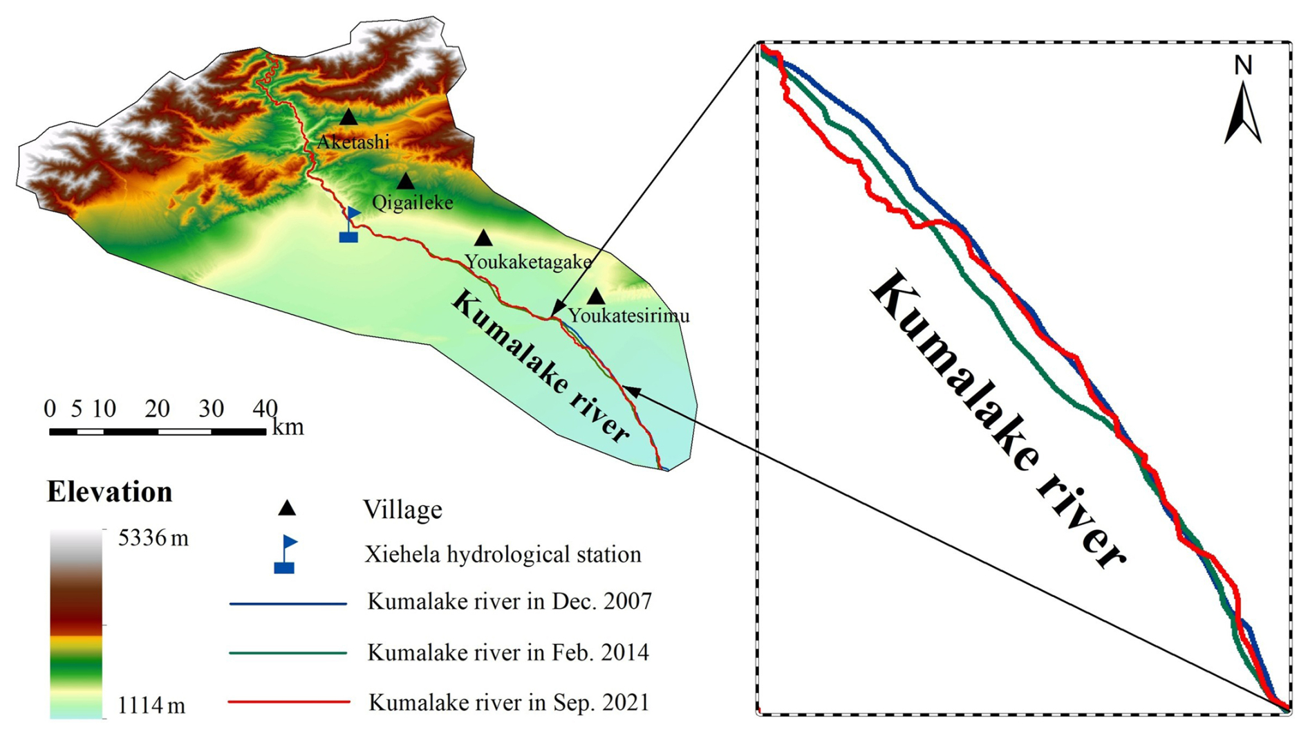
Figure 7 The spatial distribution of the Kumalake River channels in the study area.

3.4 Model settings

The outlet of the Kumalake River Basin was set at the intersection with the southeastern boundary of the study area, while all other boundaries were defined as no-flow boundaries. An unstructured triangular mesh was used to discretize the study area spatially. To accurately capture the landscape evolution processes in areas surrounding the river channel, mesh refinement was applied in the channel zones, with grid sizes less than 50 m near the river. A total of 25 968 unstructured triangular elements were generated for the study area (see Fig. 8a).

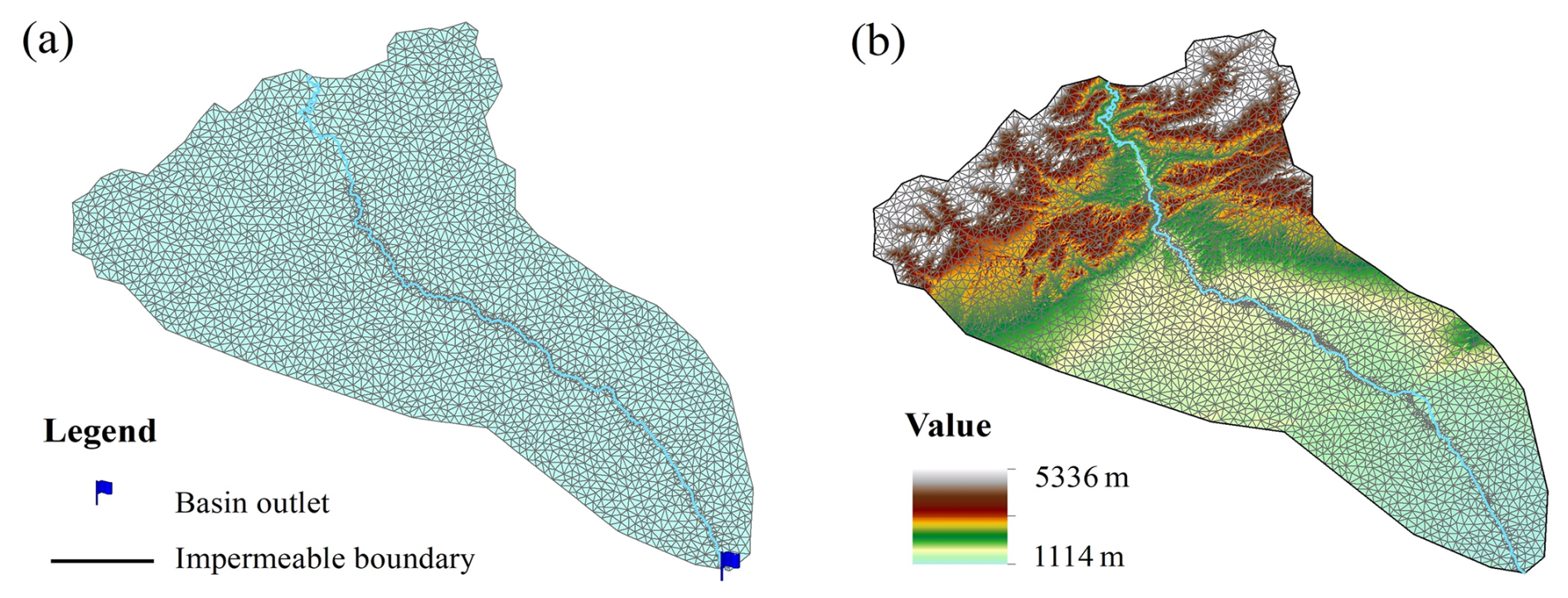
Figure 8 Mesh discretization and initial elevation grid of the research area.

The initial conditions required by LE-PIHM include ground surface elevation (Fig. 8b), canopy interception storage, snow depth, surface water depth, soil water storage, and groundwater storage. The canopy interception storage is initialized to 0 m in the model (Fig. 9 and Table 1).

The model was configured to run from January 2000–December 2021, covering a total of 264 months (22 years). To capture the seasonal variability of hydrologic processes in the study area while controlling computational load, the time step was set to one month. The LE-PIHM model was executed on an Intel Xeon E5-2680 v3 server, with an average runtime per simulation of 195 min.

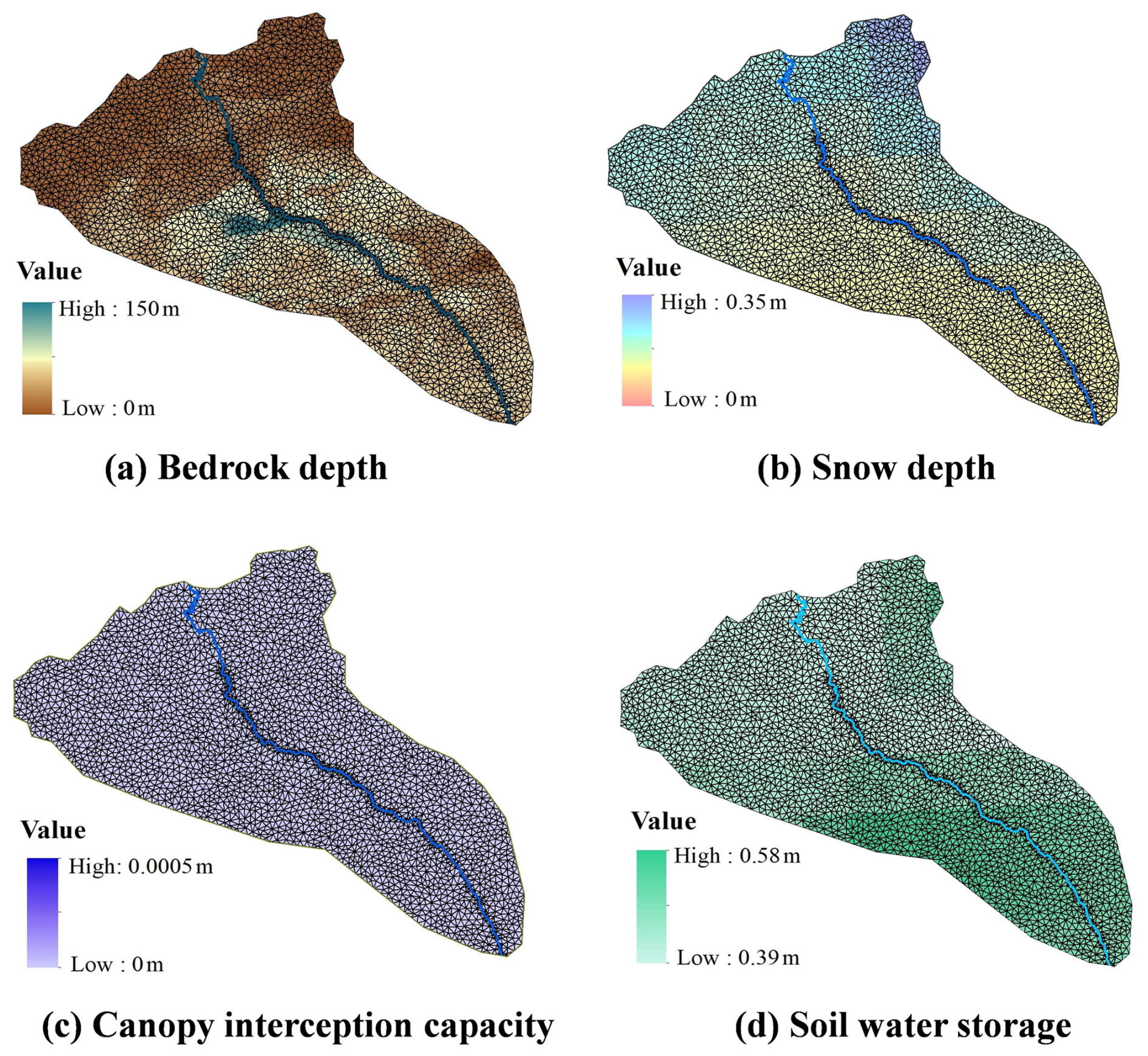
Figure 9 The initial conditions of landscape evolution model.

3.5 LSTM-based surrogate model for uncertainty analysis

After constructing the basin-scale channel migration model, the next part is to conduct parameter uncertainty analysis, followed by the reconstruction of river channel migration over 2000–2021 and the prediction of landscape evolution and river channel changes from 2021–2100 under future climate scenarios.

However, performing parameter uncertainty analysis using MCMC requires a large number of runs of the original model (i.e., the basin-scale channel migration model), which results in a significant computational burden. To reduce this computational cost, this study employs an LSTM network to construct a surrogate model for river channel migration. The surrogate model employs a two-layer LSTM architecture followed by a linear fully connected layer, with normalized LE-PIHM parameters as inputs and flattened planar river-channel coordinates as outputs, and is trained using the Adam optimizer to minimize the root-mean-square error (RMSE) loss between predicted and reference channel planforms. The main steps and more details of LSTM-based surrogated models are as follows:

• (i)

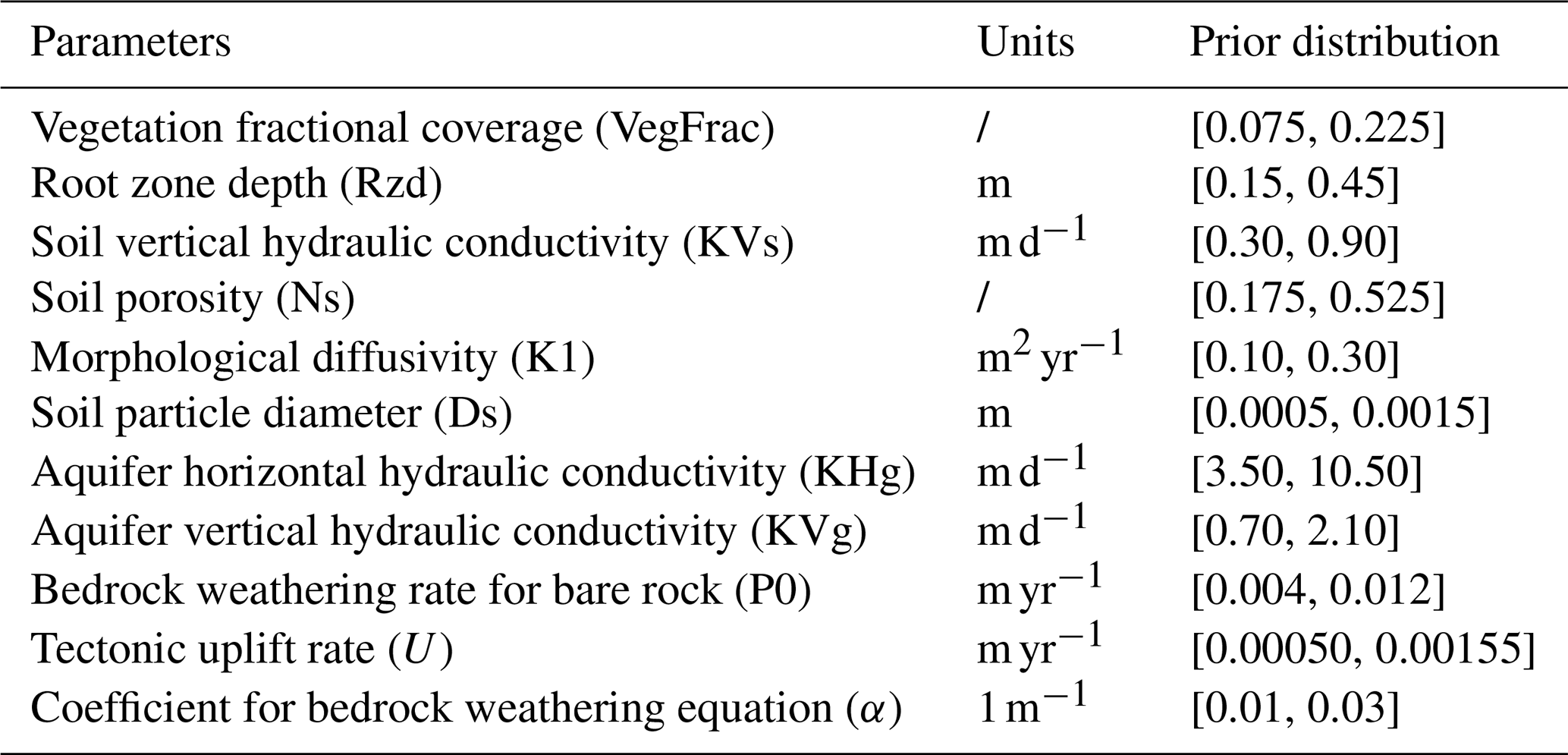
  The Sobol method is applied for parameter sensitivity analysis. Considering the property parameters of surface cover, soil, aquifer, and bedrock, 11 highly sensitive parameters LE-PIHM are selected as the input variables for the surrogate model (Table 2).

• (ii)

  Latin hypercube sampling is employed to generate 3000 sample sets within the prior ranges of the input variables.

• (iii)

  These 3000 parameter sets are individually input into the LE-PIHM model to generate surface elevation data at three time points, December 2007, February 2014, and December 2021. Subsequently, the corresponding spatial distribution of river channel is extracted through Arcpy scripting in ArcGIS. For each parameter set, the corresponding river channel is discretized uniformly into 2000 points, producing 2000 sets of planar coordinates of reaches.

• (iv)

  The obtained 3000 sets of input variables and their corresponding coordinates are split into training and validation datasets at 70 % and 30 % ratios. The LSTM network is trained to learn the nonlinear mapping between the input variables and river channel positions, thereby constructing a surrogate model for river channel migration. The network terminates in a fully connected output layer with a linear activation function and He-normal weight initialization. Training is performed using the Adam optimizer with a learning rate of $\mathrm{1}\times {\mathrm{10}}^{-\mathrm{3}}$, minimizing the root-mean-square error (RMSE) between the predicted and reference river coordinate points. The model is trained for 10 000 epochs with a batch size of 100 and a validation split of 0.1.

Table 2 The parameters of landscape evolution model and their prior ranges.

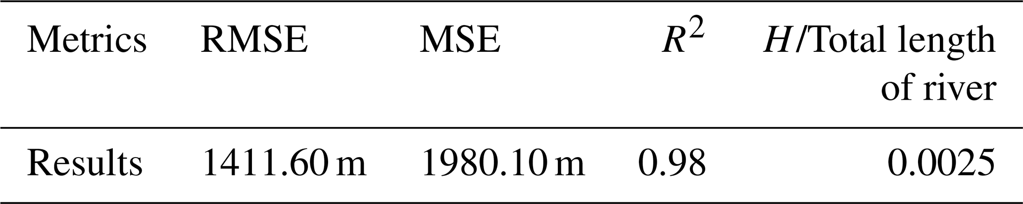
As shown in the validation results (Table 3), the surrogate model constructed using LSTM demonstrates great predictive performance for river channel locations (i.e., the planar coordinates of river reaches). It achieved a mean absolute error (MAE) of 1411.16 m, a root mean square error (RMSE) of 1980.10 m, and a coefficient of determination (R²) of 0.983. Furthermore, the average Hausdorff distance of the entire river between the surrogate model and original model outputs is 229.71 m. Given the total length of river channels in the study area is 89 337.95 m, this corresponds to only 0.25 %. Thus, these results demonstrate that the surrogate model for basin-scale river channel migration exhibits high accuracy and reliability and can replace the original model for river channel dynamics simulation.

Table 3 Evaluations of the surrogate model for basin-scale river channel migration.

The spatial distribution of river channels predicted by the original model and the surrogate model are compared across three time points (Fig. 10). The surrogate model closely matches the original in the middle and upper reaches of the river channel, while some deviations occur in the downstream reaches. This discrepancy is primarily due to the mountainous topography upstream, where the landscape is rugged and river channels are relatively stable. In contrast, the downstream region is a flat plain, where river channel migration is highly sensitive to model parameters, leading to slightly reduced accuracy in the surrogate model's performance in that area.

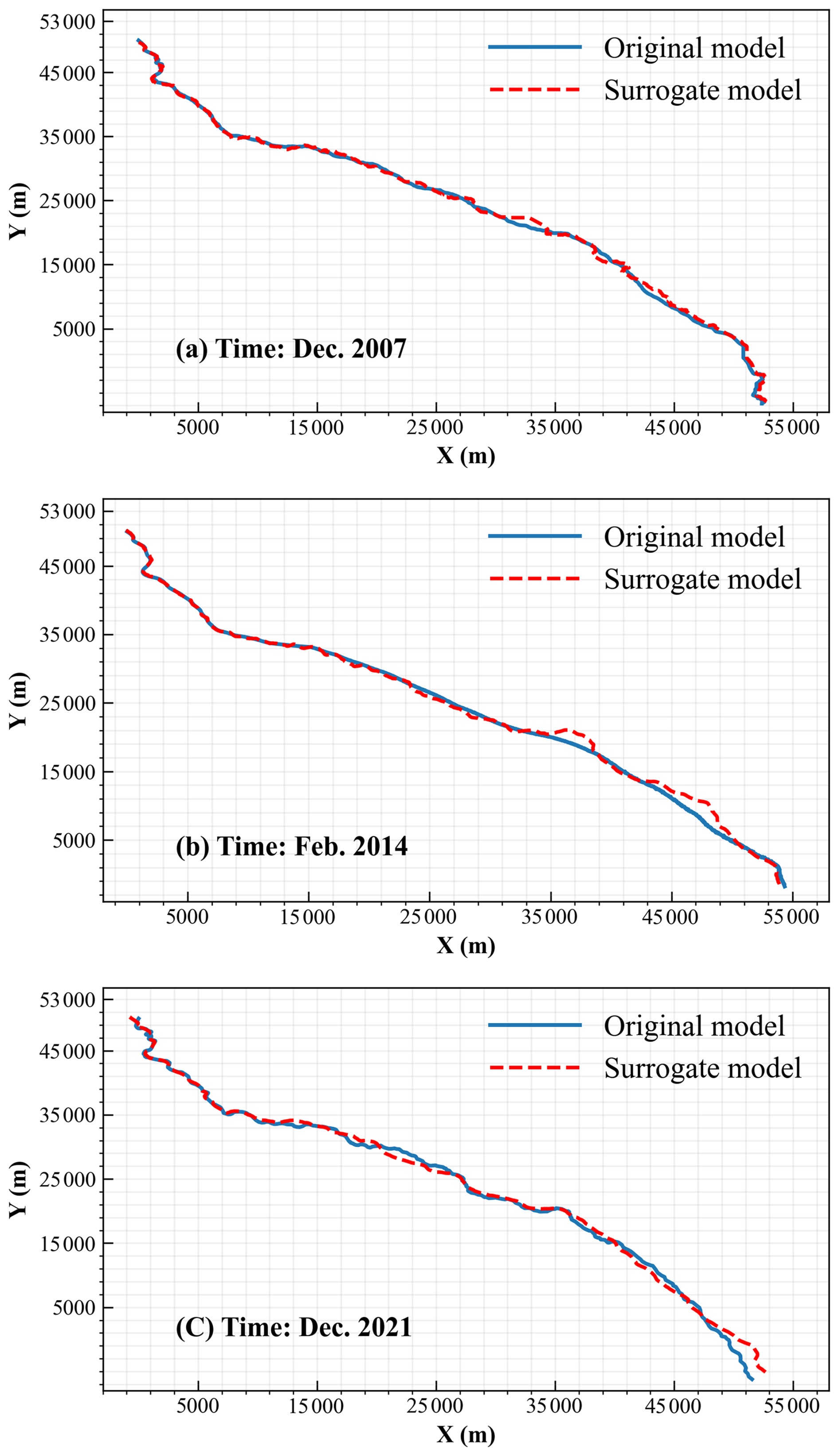
Figure 10 Comparison between the original river channel migration model and the surrogate model at different time points.

Compared to the original model, the surrogate model for basin-scale river channel migration achieves approximately a 20 000-fold increase in computational speed. Therefore, employing this surrogate model in the parameter uncertainty analysis of river channel migration can significantly reduce computational costs and effectively alleviate the computational burden associated with the uncertainty analysis process.

4 Results and discussion

4.1 Parameter uncertainty analysis

4.1.1 MCMC configuration

The river channel migration model includes 11 unknown parameters to be identified, with their prior distributions assumed to be uniform within the specified range (Table 2). The MCMC simulation is performed using the DREAMzs sampling algorithm, with three parallel Markov chains. Both the burn-in and formal sampling stages consist of 2000 iterations. Additionally, the evolution of the Markov chains employs the modified likelihood function described in Sect. 2.3.2. Based on the inferred posterior distributions of the parameters, the posterior distribution of the river channel is obtained.

4.1.2 Posterior distributions of model parameters

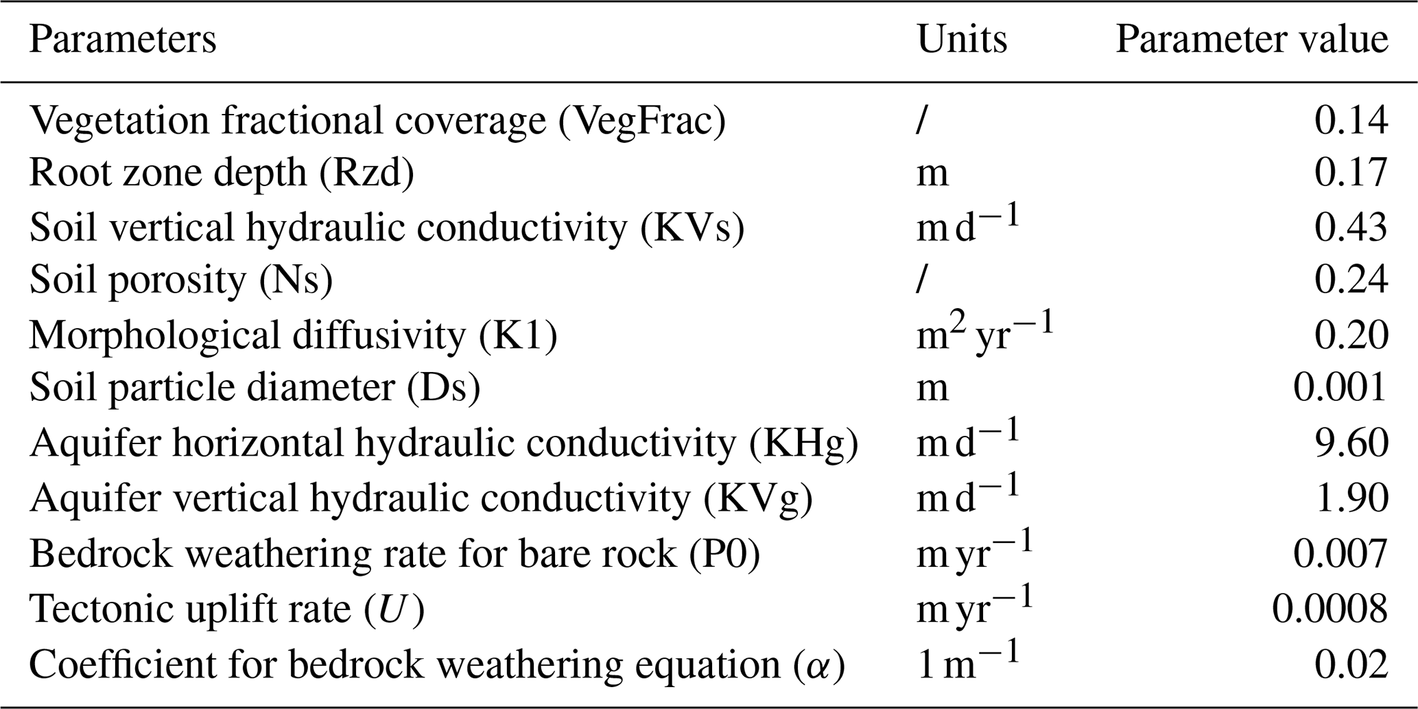
The posterior probability density histograms of the river channel migration model parameters through MCMC (horizontal axis indicates the corresponding prior ranges; Fig. 11), together with the maximum likelihood parameter set (Table 4). It is easy to find that several parameters, such as the vertical soil hydraulic conductivity (KVs), hillslope diffusion coefficient (K1), bare-bedrock weathering rate (P0), soil grain size (Ds), and vegetation fraction (VegFrac) exhibit clear convergence to relatively narrow and concentrated posterior ranges after calibration. This suggests that channel-planform predictions are highly sensitive to these parameters, and that they exert strong control on basin-scale erosion-deposition balance and channel migration behavior.

Figure 11 Calibrated posterior distributions of model parameters.

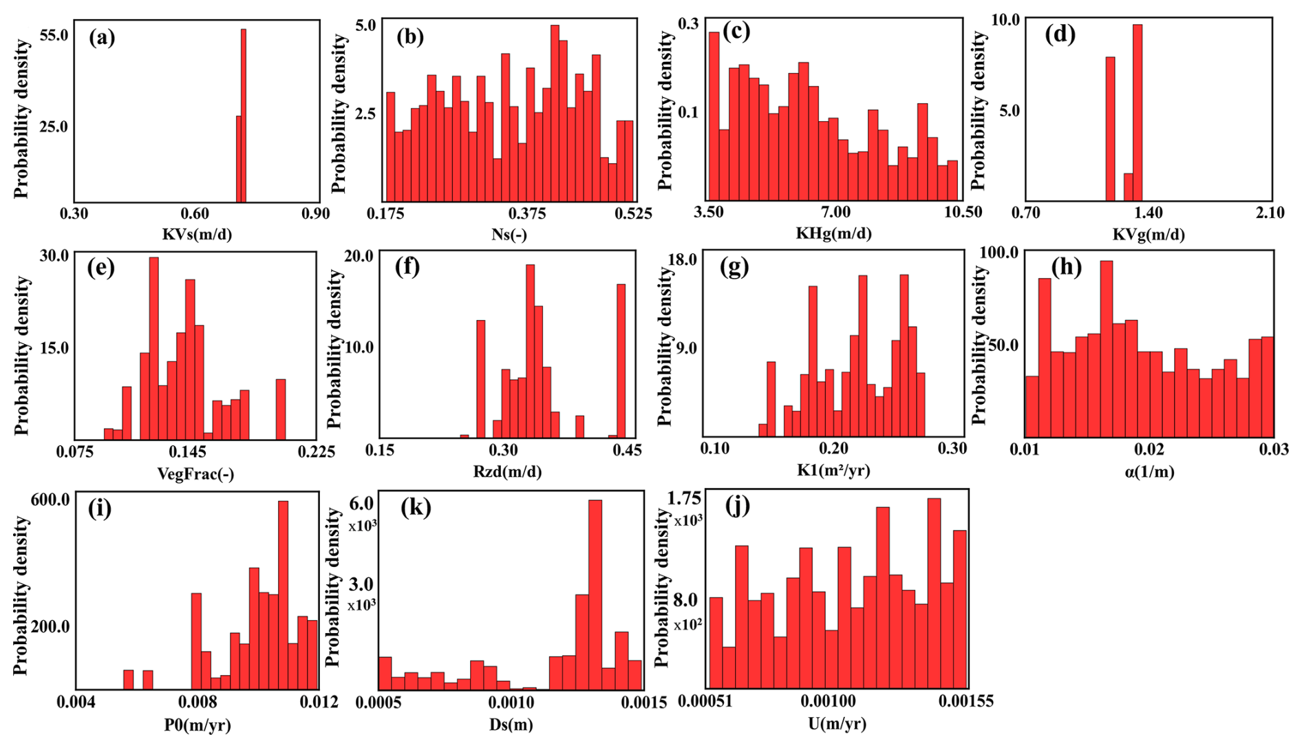
Table 4 Parameter set corresponding to the maximum likelihood estimate.

In contrast, the posterior distributions of some parameters, such as aquifer horizontal hydraulic conductivity (KHg), the weathering-law coefficient (α), and the tectonic uplift rate (U), remain comparatively broad. This indicates that, given the spatial scale of this study and the available observational constraints, channel-planform position is less responsive to these parameters. Over the past 22 years, channel migration in the basin scale may have limited sensitivity to tectonic uplift, or the effects of uplift may be partially compensated by other parameters within the coupled hydro-geomorphic system.

4.1.3 Reconstruction of river channel migration (2000–2021)

Based on the posterior distributions of the identified parameters, the river channel evolution from 2000–2021 in the study area was reconstructed. The result shows that the predicted confidence interval fully encompasses the observed river channel (Fig. 12), and the blue shaded region denotes the 95 % confidence interval, the red line represents the observed river channel in Fig. 12. The average Hausdorff distance of the entire river between the simulated channel (marked in black line in Fig. 12) with the maximum likelihood parameter set and the observed channel is 225.42 m, which accounts for only 0.25 % of the total river channel length. This indicates that the discrepancy between the simulated and observed river channel per unit length is minimal, demonstrating the high accuracy of the calibrated river channel migration model. Therefore, the river channel model facilitated by Bayesian parameter uncertainty quantification can reliably predict the river channel migration processes within the study area.

Figure 12 The predicted Kumalake River channel at December 2021.

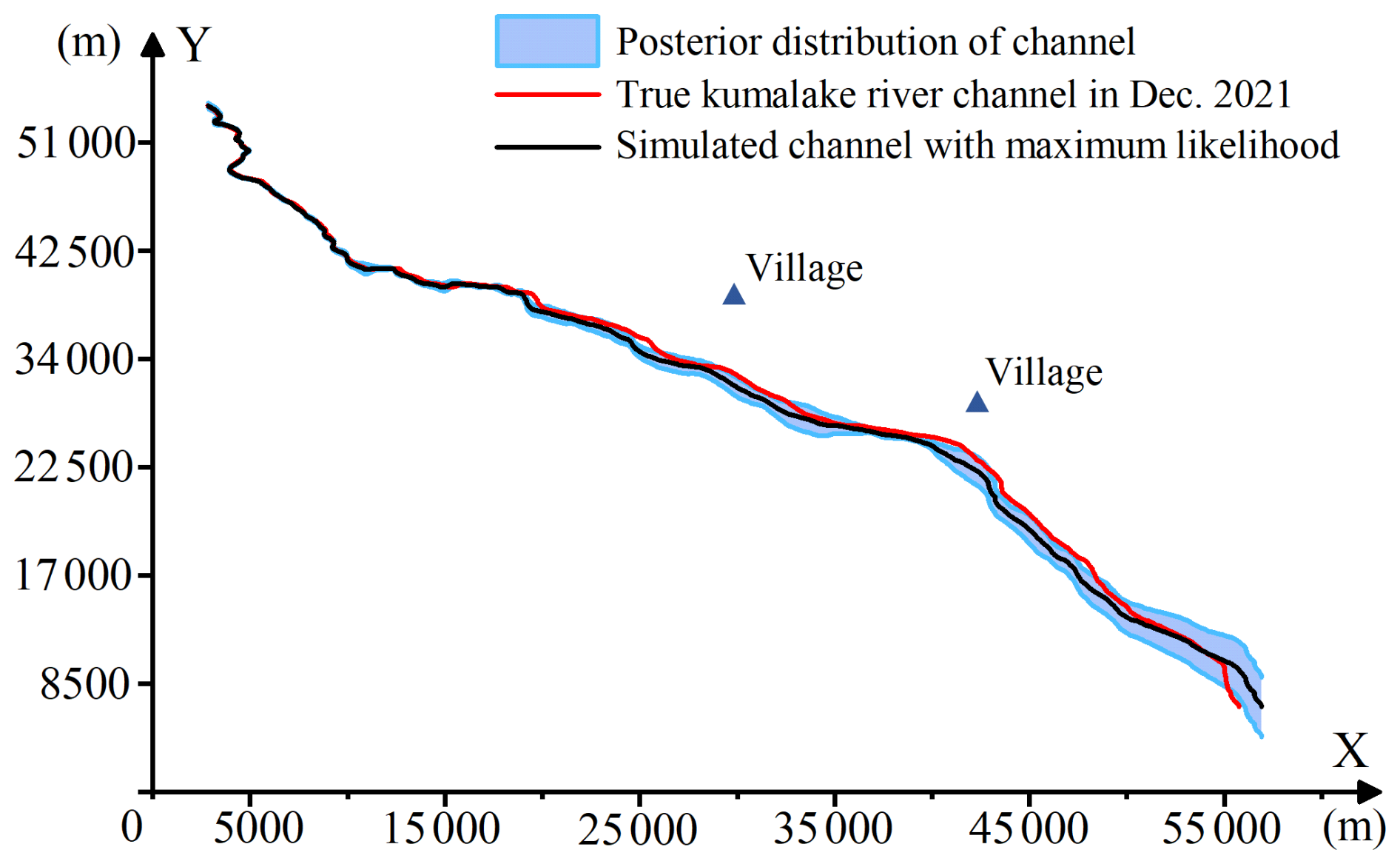
Remote sensing images (Fig. 13) collected during the simulation period of the study area indicates that, beginning in 2012, the villages along the river initiated to develop cultivated land near the river channel. This anthropogenic activity altered key parameters related to land cover and soil type, and may have been a driving factor for the gradual southward migration of local river reaches. However, this mechanism of human-induced change is not explicitly represented in the landscape evolution model, which may partly explain the reduced simulation accuracy in the downstream region. Nevertheless, the parameter uncertainty analysis conducted in this study helps to partially compensate for the effects of land reclamation, keeping the prediction deviation of basin-scale river channel migration model within an acceptable range.

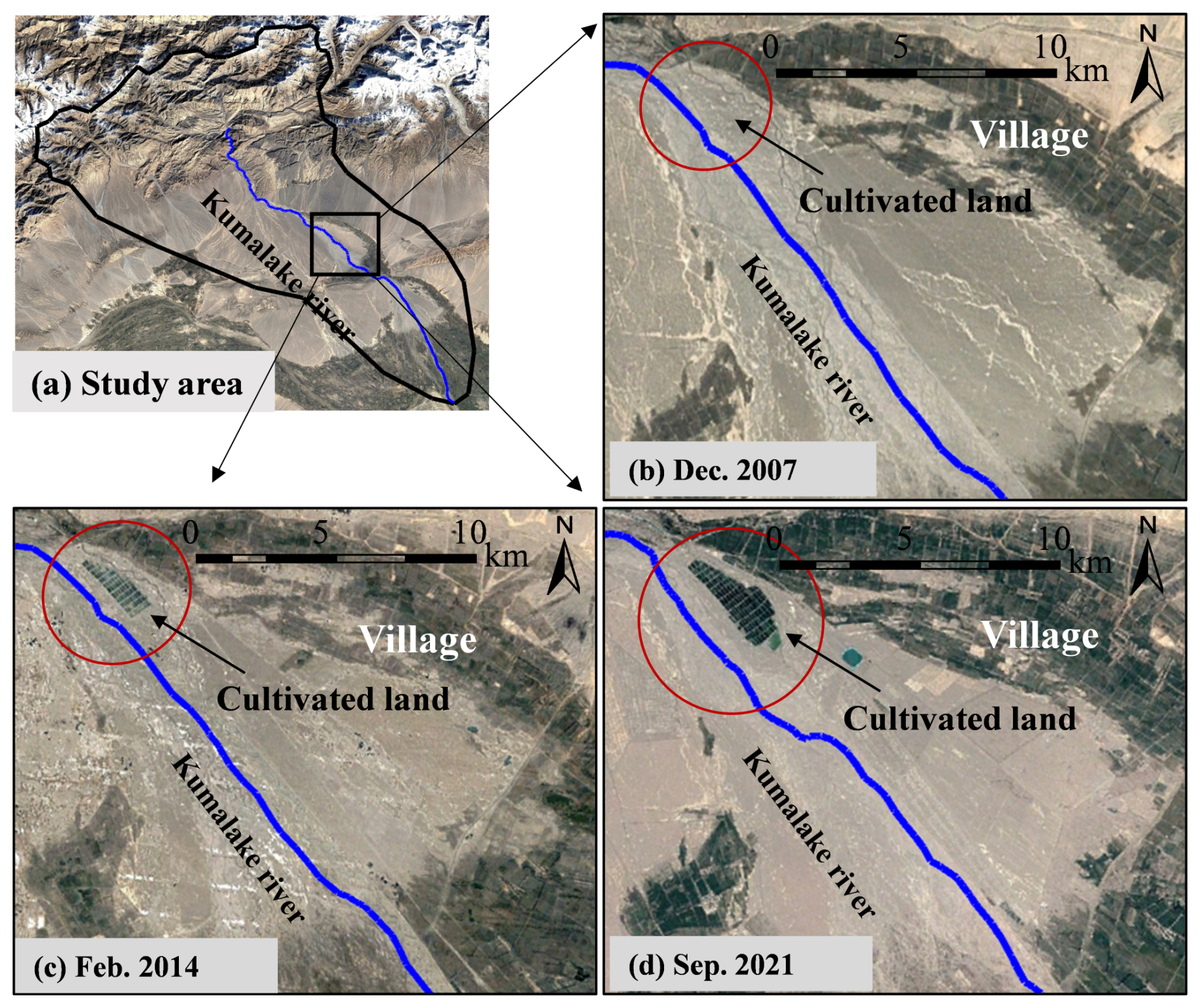
Figure 13 Formation process of cultivated land along the river in the study area. Satellite imagery from Google Earth Pro (Imagery © Landsat/Copernicus; Map data © Google), modified by the authors.

4.2 Prediction of river channel migration in future (2021–2100)

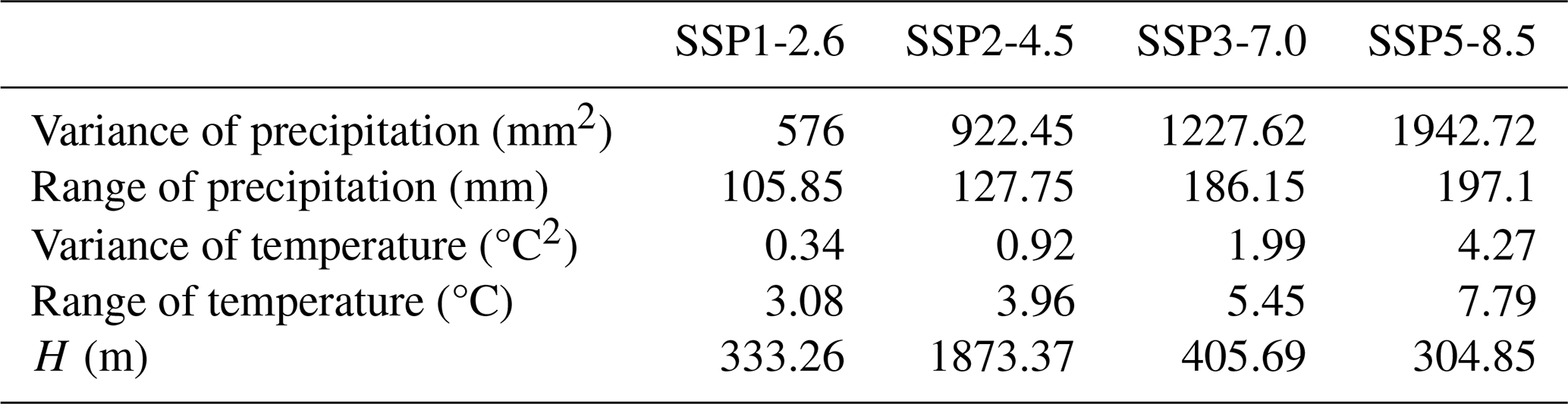
Future climate change will influence landscape evolution and river channel migration, thereby affecting regional water resource patterns and ecological environments. The EC-Earth3-Veg climate model, released under phase 6 of the Coupled Model Intercomparison Project (CMIP6), incorporates vegetation-climate interactions and is well-suited for evaluating terrestrial ecosystem and hydrological responses under different climate scenarios (Alsalal et al., 2024; Eyring et al., 2016). Based on the EC-Earth3-Veg model, this study adopts four scenarios of shared socioeconomic pathways (SSPs), i.e., SSP1-2.6, SSP2-4.5, SSP3-7.0, and SSP5-8.5. Each of the four climate scenarios reflects a distinct pathway of global socioeconomic development and associated impacts on greenhouse gas emissions and climate change (O'Neill et al., 2016).

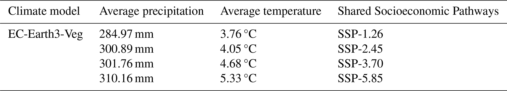
The scenario forcing fields are mapped to the LE-PIHM basin computational units using bilinear interpolation. To maintain consistency with the monthly time step adopted in LE-PIHM, the forcing data are temporally aggregated to monthly resolution prior to being used as model inputs. Scenario-based simulations of landscape evolution and river channel migration were conducted by using these climate conditions as the driving force of LE-PIHM. The climate conditions for these scenarios over the period (2021–2100) are characterized by the annual mean temperature and precipitation (Table 5 and Fig. 14).

Table 5 Statistics of four climate scenarios under the EC-Earth3-Veg model.

Figure 14 Annual mean precipitation and temperature for the four climate scenarios.

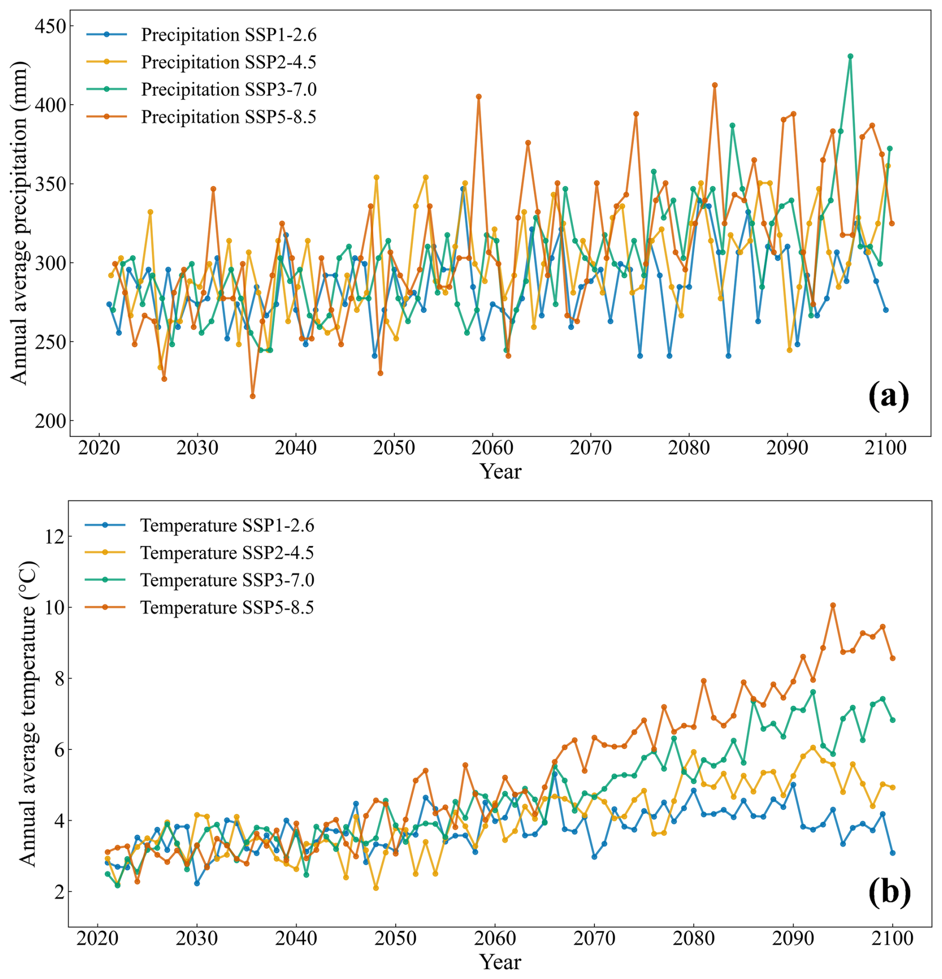
Using LE-PIHM and the parameter set corresponding to the maximum likelihood estimate (Table 4), the landscape evolution and river channel migration from 2021–2100 were simulated for the study area under four climate change scenarios. After 80 years of simulated landscape evolution, the overall topographic pattern of the region remains characterized by higher elevations in the north and lower elevations in the south, with elevation changes ranging from +1.39 m to −0.37 m. The simulation results under the four EC-Earth3-Veg climate scenarios demonstrate that the elevation change and river channel migration in basin scale by the year 2100 exhibit distinct characteristics (Fig. 15a). In the northern mountainous area, distinct alternating patterns of uplift and subsidence are observed, with relatively large magnitudes of change. This is primarily due to intense bedrock weathering and steep slopes in the mountains, where the regolith layer is thin and the weathered soil and sediment are prone to downslope transport into adjacent low-lying regions, resulting in significant elevation fluctuations. In contrast, the southern plain exhibits gentle topography and minimal elevation differences, making it less conducive to large-scale sediment transport. As a result, the landscape undulation in the plain is relatively mild and limited in amplitude.

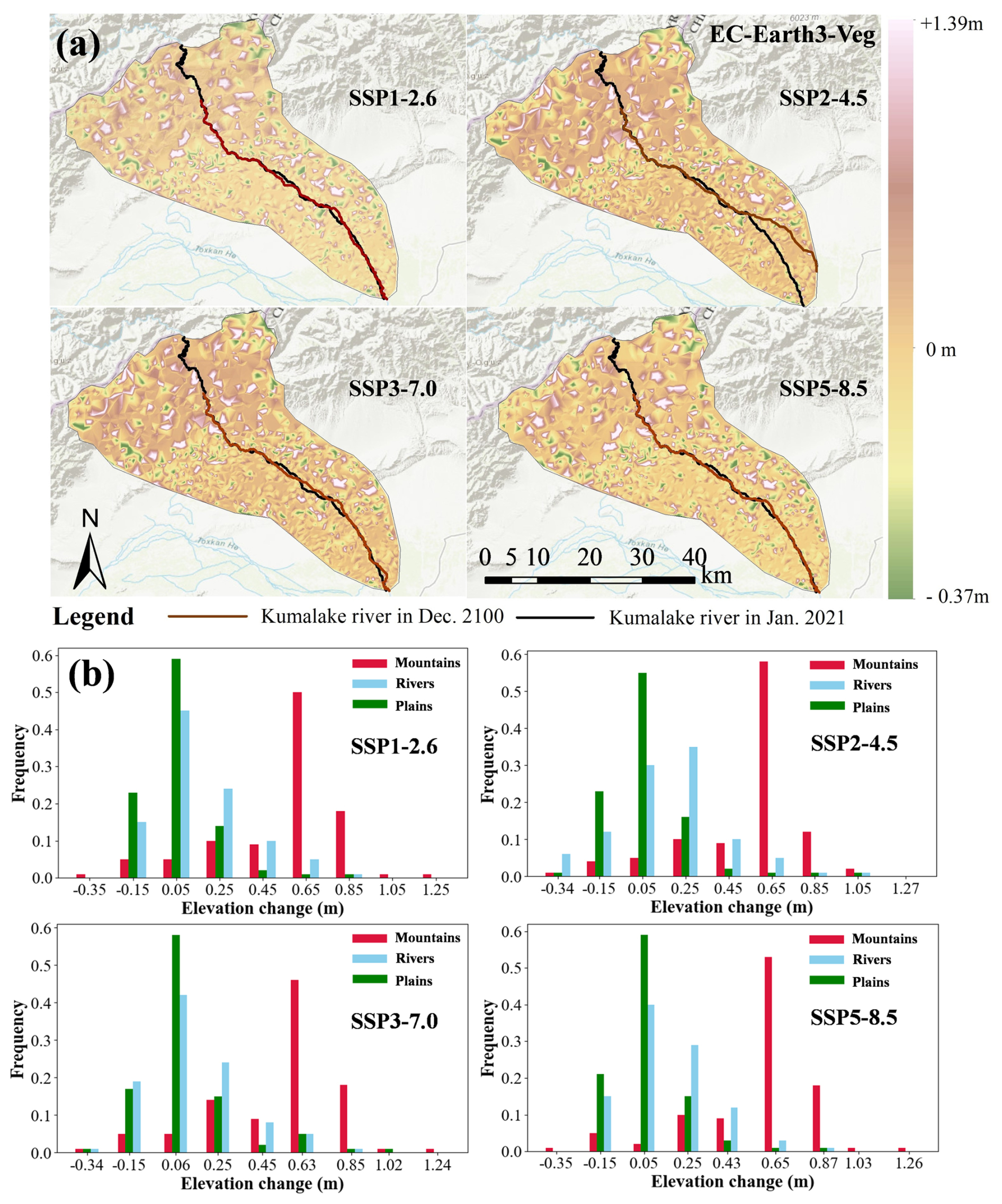
Figure 15 Spatial distribution of river channel (a) and Elevation change (b) under four future climate scenarios based on the EC-Earth3-Veg climate model. Basemap: Esri World Hillshade | Powered by Esri.

Under the EC-Earth3-Veg climate model, the four future climate scenarios induce distinct patterns of river channel migration. By the end of the simulation period (2100), the upstream reaches of the Kumalake River remain largely unchanged from their 2021 positions. This stability is attributed to the fact that these reaches flow through narrow and geomorphologically stable canyon landscape, where external disturbances are minimal and the river alignment and morphology remain relatively constant. In contrast, several downstream reaches situated in the plain exhibit varying degrees of northward migration. This phenomenon is mainly driven by the relatively gentle topography of the plains, increased sediment deposition, redistribution of flow energy, and anthropogenic activities. These factors collectively lead to channel swinging, incision, or aggradation, gradually shifting the river channel position.

The four scenarios under EC-Earth3-Veg exhibit significant differences in temperature and precipitation characteristics, as well as in the extent of river channel migration (Table 6). Notably, under the SSP2-4.5 scenario, although the climate variability is not the most intense among the scenarios, the elevation change shows the largest amplitude, and the topographic changes in the river area are more pronounced (Fig. 15a), leading to a shift of the downstream river channels into the plain area. This suggests that the climate changes in this scenario trigger a sudden and intense spatial reorganization of the river network, resulting in significant morphological transformation. The specific combination of climatic conditions may cause the river system to approach an evolutionary threshold (Church, 2002; Meyer et al., 2018). When such a critical threshold is reached, the river system may undergo abrupt transitions, manifesting as regime shifts (Church, 2002).

Table 6 Statistics of climate scenarios and average Hausdorff distance of river migration.

In summary, within the LE-PIHM landscape evolution framework, channel planform dynamics and elevation changes are jointly controlled by the following processes. (i) Precipitation-runoff mechanisms, including rainfall, infiltration and runoff generation, and surface-groundwater exchange; (ii) Sediment supply and transport capacity, including hillslope diffusion, weathering-driven sediment production, and river sediment transport; (iii) Landscape-flow-routing feedbacks, whereby landscape evolution and the associated adjustment of D8-based flow paths modify local slope and discharge concentration.

These results indicate that the process of river channel migration in the study area under climate forcing varies across scenarios. Future climate conditions play a critical role in regional landscape evolution and river dynamics. Furthermore, the complex feedbacks between climate change and geomorphic systems highlight the importance of incorporating these interactions in predictive modeling of fluvial landscape evolution and watershed management planning.

5 Conclusions

River channel migration at the basin scale not only determines the spatial distribution pattern of regional river networks, but also exerts profound influences on local ecosystems and the development of civilizations within the basin. Simulating river channel migration at the basin scale aids in quantitatively reconstructing this long-term, complex dynamic processes and also provides a scientific basis for decision-making in response to climate change and natural disasters. To address the limitations of traditional river channel migration models in temporal and spatial scale applications, this study integrates a landscape evolution model with river channel extraction techniques, achieving accurate and reliable simulation of river channel migration processes at the basin scale. Using the Kumalake River Basin as a case study, the river channel migration process in the region is reconstructed based on the LE-PIHM landscape evolution model and river channel extraction techniques. The main conclusions of this study are as follows:

1. The LSTM-based surrogate model for river channel migration demonstrates high accuracy and effectively overcomes the computational challenge associated with parameter uncertainty analysis. The parameter calibration using MCMC requires numerous executions of the LE-PIHM model and river channel extraction, resulting in prohibitive computational demands. The surrogate model for basin-scale river channel migration based on LSTM networks accurately characterizes the response relationship between landscape evolution parameters and river channel locations, effectively solving the problem of computational burden in Bayesian uncertainty analysis.

2. The river channel migration model facilitated by Bayesian parameter uncertainty quantification can reliably predict the river channel evolution process within the study area. Based on the inferred posterior distributions of model parameters, the predicted confidence interval of the channel fully encompasses the actual river location. The average Hausdorff distance between the simulated river channel with the maximum likelihood parameter set and the observed river channel is 225.42 m, which accounts for only 0.25 % of the total channel length. Thus, the basin-scale river channel migration model incorporating Bayesian uncertainty analysis demonstrates high reliability and predictive capability, enabling effective characterization of river migration processes within the study area.

3. River channel evolution under different climate scenarios demonstrates significant variability, and future climate change will profoundly affect basin geomorphological characteristics and river network configurations. Based on the EC-Earth3-Veg model released by CMIP6, the landscape evolution and river channel migration in the study area from 2021–2100 were projected under four Shared Socioeconomic Pathways (SSP1-2.6, SSP2-4.5, SSP3-7.0, and SSP5-8.5). The results indicate that climate change and geomorphological systems exhibit complex response mechanisms.