DAR-type model based on “long memory-threshold” structure: a competitor for daily streamflow prediction under changing environment

The non-stationarity and non-linearity of streamflow have increased with changes of the environment, challenging accurate streamflow prediction. Furthermore, the overlook of long-term memory features could lead to biases in model parameter estimation and testing of time series properties. The classical linear Autoregressive-Generalized Autoregressive Conditional Heteroskedasticity (AR-GARCH) model has a narrow parameter range, and the moment conditional requirements for parameter estimation are relatively strict, limiting its applicability and prediction accuracy in modeling and predicting daily streamflow. Under the premise of long-term memory, a dual-threshold double autoregressive (DTDAR) model is proposed to capture the non-linear patterns in streamflow series. Using 15 hydrological stations in the Yellow River basin in China as an example, DTDAR models are compared with AR-GARCH and long short-term memory (LSTM) models to assess their applicability and predictive ability. The results indicate that the DTDAR models have a stronger predictive ability for daily streamflow than the AR-GARCH-type and LSTM models. The nonlinear changes of the daily streamflow time series are reflected in multiple linear structures by adding the threshold, improving the accuracy of the single linear structure method. The NSE values of the FDTDAR and TAR-GARCH models are higher than those of the DAR and AR-GARCH models by 0.013–0.556 and 0.031–0.582, respectively. Compared to the normal distribution, the Student's t distribution for residuals is a better choice for predicting daily streamflow time series in the study area. This study enriches the stochastic hydrological models and improves the accuracy of streamflow prediction.

1 Introduction

The behavioural characteristics of hydrological systems have become increasingly complex in the face of climate change and human activities (Lyu et al., 2023; Ma et al., 2024; Matic et al., 2022; Sivakumar, 2009). Time series analysis method has gained wide attention in hydrological simulation and prediction due to its outstanding ability to describe the structure, function, and development trend of the system, and has become one of the hot issues in stochastic hydrology research (Can et al., 2012; Chen et al., 2021; Yang et al., 2022). As such, several stochastic models have been proposed, among which the regression model has a simple form and is easy to implement.

Traditional regression models, including the autoregressive (AR) model, the moving average (MA) model, and their combined form (ARMA model), are well-suited for stationary time series but have significant limitations. For non-stationary series, the differencing ARMA (ARIMA) model is an effective method, and its key difference from the ARMA model is the addition of a difference step to smooth the sequence (Wang et al., 2019). However, both the ARIMA and ARMA models struggle to handle seasonality in time series. The seasonal ARIMA (SARIMA) model is the preferred option for monthly streamflow time series with annual cycles resulting from seasonal variations (Adnan et al., 2019; Modarres, 2007). However, the illegible seasonal features in the daily streamflow series bring a challenge to the applicability of the SARIMA model. To overcome this issue, seasonal standardization is necessary to preprocess daily streamflow time series, removing the influence of seasonality for subsequent research (Guo et al., 2021a).

In the last decades, the conditional heteroscedastic behaviour (ARCH effect) of the mean model residual series obtained increasing attention due to changing environment (Guo et al., 2021b; Nazeri-Tahroudi et al., 2022; Wang et al., 2023a). The generalized Autoregressive Conditional Heteroscedasticity (GARCH) model has been often employed to improve the modelling accuracy of the AR-type model by eliminating the ARCH effect in the residuals (Fathian et al., 2018; Fathian and Vaheddoost, 2021; Pandey et al., 2019; Zha et al., 2020). However, the AR-GARCH model, a typical regression model for streamflow forecasting, has a more cumbersome combined form than a single model, hindering its application. Compared with the AR-GARCH, the double autoregressive (DAR) model proposed by Ling (2007) is more concise in form, can describe the first- and second-order moments behaviour of time series simultaneously, and has been applied maturely in the economic field (Hansen, 2021; Jiang et al., 2020; Li et al., 2019; Liu et al., 2018). In addition, the AR model requires the autoregressive and moving average parameters to fall within the range of −1–1, and the sum is lower than 1, while the GARCH model restricts non-negative values and the sum (except for the constant) is below 1. In contrast, the definition range of the DAR model parameter is broader, with first-order moment selection throughout the real number field and non-negative second-order moment constraints. However, the DAR model has not yet been applied in the field of hydrology, and its prediction performance has not been verified.

Dimitriadis and Koutsoyiannis (2015) demonstrated that long-term persistence – characterized by the temporal dependence between historical and contemporary streamflow – is fundamental to daily streamflow prediction. And it has been reported that time-varying volatility detected in daily streamflow series could be attributed to long-term memory (Dimitriadis et al., 2021; Graves et al., 2017; Grimaldi, 2004), which may lead to a spurious ARCH effect in residuals of the pure AR model, rendering the constructed GARCH model insufficient and affecting prediction performance. Both the combined AR-GARCH model and the novel DAR model are powerless to reproduce the long-term persistence of the daily streamflow time series. Long-term memory was always neglected in the vast majority of existing streamflow simulation and prediction studies. The research on long memory began with Hurst (1951) and Mandelbrot and Wallis (1969), and Hurst proposed the Hurst index (H, H>0.5 indicates that the time series has long memory) to identify it. Although this characteristic was initially identified within the field of hydrology, at that time, there lacked a research methodology widely recognized by most hydrologists that could effectively reproduce the long-term memory of daily streamflow. Granger (1978) proposed the concept of “fractionally differencing”, which laid the foundation for the development of later long-memory models (such as the ARFIMA model). Hosking (1981) followed up in the field of hydrology. Montanari et al. (1996, 1997) still believed that the fractional difference model is the only method to describe the daily streamflow time series with long-term persistence.

Hydrological time series are highly nonlinear, as proven in numerous studies (Delforge et al., 2022; Feng et al., 2022; Guo et al., 2021b; Miller, 2022; Yuan et al., 2021), which poses significant challenges to traditional mean models (e.g., AR, ARMA). The threshold autoregressive model based on the AR model can capture and predict the nonlinearity in the mean behaviour of hydrological time series (Tong, 1983). Several recent studies (Fathian et al., 2019; Gharehbaghi et al., 2022; Huang et al., 2021; Kolte et al., 2023) have introduced a new combination model coupled with the nonlinear mean model, namely artificial intelligence-GARCH, for prediction work. Guo et al. (2021b) combined the Self-Exciting TAR model with the GARCH model to predict groundwater depth and achieved satisfactory prediction accuracy. However, the applicability of the TAR-GARCH model to hydrological time series is limited by narrow parameter constraints (Guo et al., 2021b; Li et al., 2016).

This study aims to improve the prediction accuracy of daily streamflow time series by constructing a novel model with high applicability that can simultaneously capture seasonality, non-stationarity, long-term memory, and nonlinearity of daily streamflow. We propose the Fractional-differenced Dual-Threshold Double Autoregressive (FDTDAR) framework that systematically integrates seasonal normalization, fractional differencing for long-memory modeling, and a dual-threshold structure to capture regime-specific nonlinearities. Furthermore, we evaluate alternative residual distributions – comparing the standard Gaussian distribution against the heavy-tailed Student's t-distribution – to improve residual characterization. The framework is applied to daily streamflow data from 15 gauging stations located in the Yellow River Basin. For robust evaluation, the historical data are divided into a 70 % calibration period and a 30 % out-of-sample testing period to assess the one-day-ahead forecasting performance. The FDTDAR framework is rigorously evaluated against both the classical linear AR-GARCH model and the long short-term memory (LSTM) network. Evaluation metrics include Mean Absolute Error (MAE), Root Mean Squared Error (RMSE), Coefficient of determination (R²), Nash-Sutcliffe efficiency coefficient (NSE), and Absolute Maximum Error (AME), providing a multi-faceted assessment of model robustness.

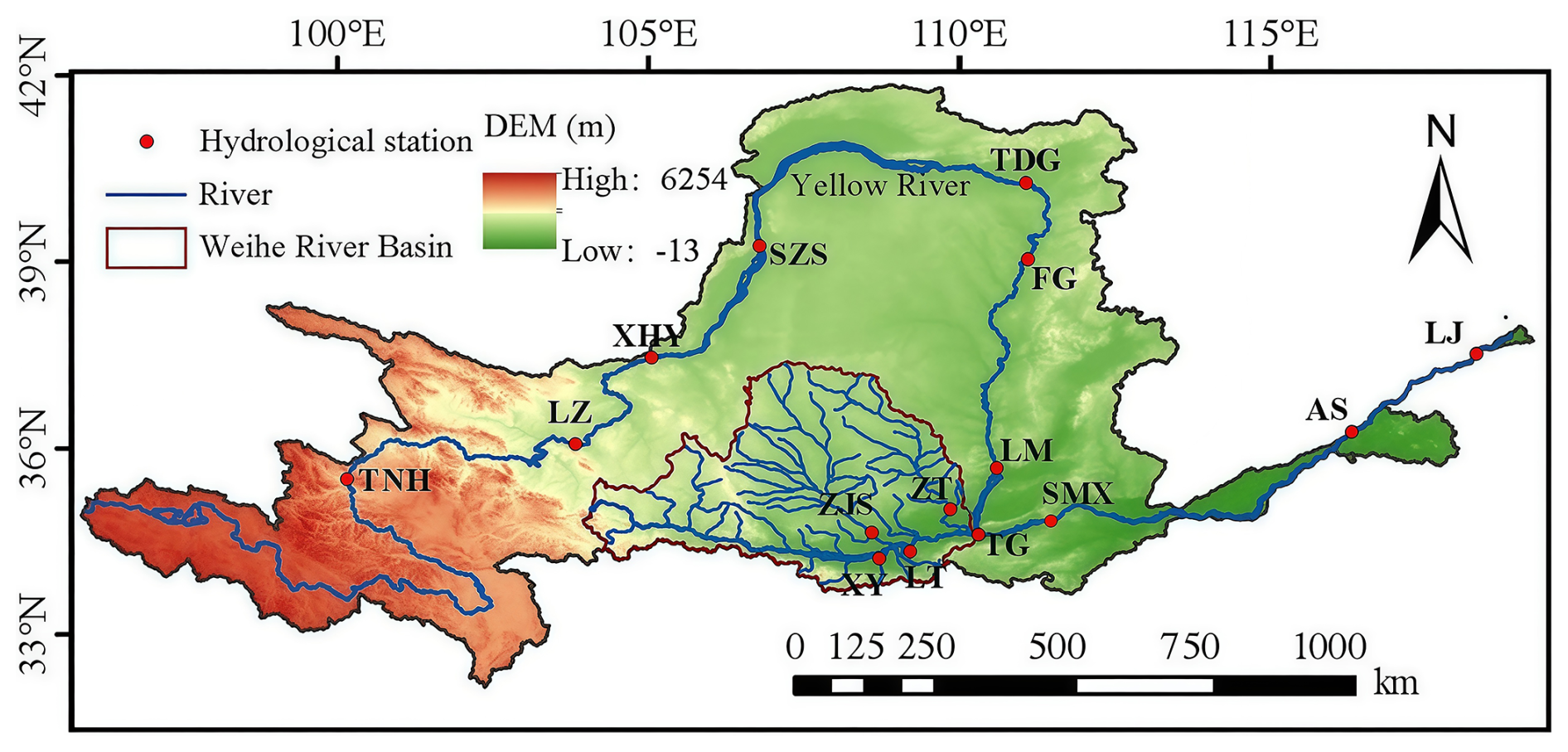
Figure 1 The Yellow River basin and locations of 15 hydrological stations.

2 Study area and data

2.1 Study area

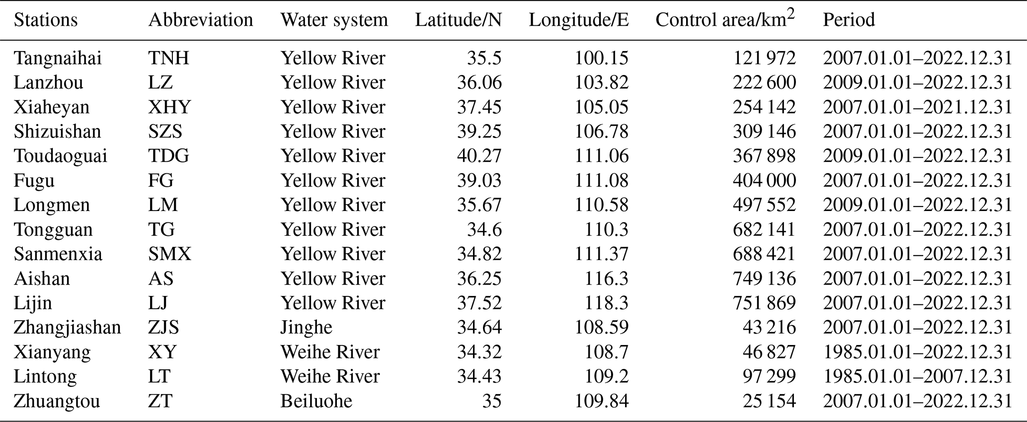
The research area of this study (Fig. 1) is the Yellow River Basin in China, which has a main stream length of approximately 5464 km and a catchment area of about 795 000 km², ranking second in China and fifth in the world. The Yellow River originates from the Bayan Har Mountains in Qinghai Province, Western China, and flows through 9 provinces before emptying into the Bohai Sea. This study utilizes daily streamflow records from 15 hydrological stations in the Yellow River Basin. These stations are selected based on rigorous criteria to ensure statistical robustness: (i) a minimum continuous record length of 10 years; (ii) a data completeness requirement of 100 %, with zero missing daily values throughout the selected study period to ensure continuous time-series modeling; and (iii) spatial representativeness covering the upper, middle, and lower reaches of the basin. These stations (Fig. 1) include those located on the mainstream (Tangnaihai (TNH), Lanzhou (LZ), Xiaheyan (XHY), Shizuishan (SZS), Toudaoguai (TDG), Fugu (FG), Longmen (LM), Tongguan (TG), Sanmenxia (SMX), Aishan (AS), and Lijin (LJ)) and the largest tributary Weihe River Basin (Zhangjiashan (ZJS), Xianyang (XY), Lintong (LT), and Zhuangtou (ZT)).

2.2 Daily streamflow time series data

This study selects the measured daily streamflow time series from 15 hydrological stations in the Yellow River Basin (Table 1). Figure S1 in the Supplement depicts the temporal variation of the daily streamflow time series for the 15 hydrological stations. The daily streamflow record for each station is partitioned chronologically: the initial 70 % of the data serves as the calibration period for identifying statistical characteristics and estimating model parameters, while the remaining 30 % is reserved as an independent testing set. This setup allows for assessing the model fit during calibration and conducting a robust, out-of-sample evaluation of prediction accuracy across the various models.

Table 1 Basic information of daily streamflow series for 15 stations.

3 Methodology

3.1 De-seasonal standardization

For a given original daily streamflow time series, the mathematical expression for deseasonalization is as follows:

$$\begin{array}{}\text{(1)}& {\displaystyle }\left\{\begin{array}{l}{\mathit{\mu }}^m=\frac{\mathrm{1}}{N}{\sum }_{n=\mathrm{1}}^N{X}_t^{\left(n,m\right)}\\ {\mathit{\sigma }}^m={\left[\frac{\mathrm{1}}{N}{\sum }_{n=\mathrm{1}}^N{\left(X_t^{\left(n,m\right)}-{\mathit{\mu }}^m\right)}^{\mathrm{2}}\right]}^{\mathrm{0.5}}\end{array}\right.\text{(2)}& {\displaystyle }{Y}_t={\displaystyle \frac{X_t-{\mathit{\mu }}^m}{{\mathit{\sigma }}^m}}\end{array}$$

where $X_t^{\left(n,m\right)}\left(n=\mathrm{1},\mathrm{\dots },N;m=\mathrm{1},\mathrm{\dots },M\right)$ (M=366 in a leap year and 365 in a normal year) is the original daily streamflow time series of the mth day in the nth year, μ^m and σ^m are the mean and standard deviation of the variable for each calendar day, respectively; Y_t ($t=\mathrm{1},\mathrm{\dots },T)$ represents the daily streamflow time series after removing seasonality, and the training period length is T.

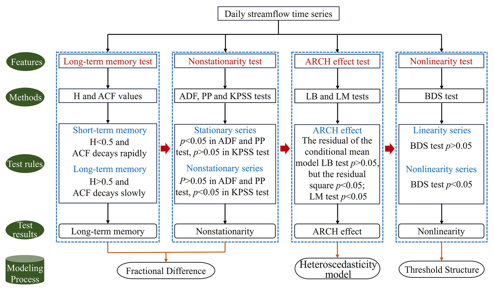
Figure 2 Schematic flowchart of the analysis pipeline, illustrating the sequence of statistical diagnostic tests and the motivated selection of the FDTDAR framework components.

3.2 Statistical diagnostic methods for streamflow series

Before initiating the modeling procedure, it is essential to understand the inherent statistical properties of daily streamflow time series. The primary objective of this section is to introduce a comprehensive diagnostic analysis to evaluate four key characteristics of time series: long-term persistence, non-stationarity, ARCH effects, and nonlinearity (Fig. 2). These features are critical in determining the suitability and effectiveness of various modeling approaches. Moreover, understanding their interconnections provides important theoretical support for the logical consistency and robustness of the subsequent modeling framework (Fig. 2).

The daily streamflow time series exhibits seasonal characteristics due to the cyclical influence of the four seasons. Therefore, deseasonalization is a necessary preprocessing step before modeling. In this section, the presence of long-term memory in the daily streamflow series is identified by the Hurst exponent (H) calculated using the rescaled range (R/S) analysis method and the trend of the autocorrelation function (ACF). The influence of seasonality on long-term memory is also assessed (Lo, 1991). On this basis, the stationarity of the series is evaluated using three unit root tests: the Augmented Dickey-Fuller (ADF), Phillips-Perron (PP), and Kwiatkowski-Phillips-Schmidt-Shin (KPSS) tests (Dickey and Fuller, 1981; Kwiatkowski et al., 1992; Peter and Perron, 1988). The null hypotheses of the ADF and PP tests assume that the time series has a unit root, while the KPSS test considers the null hypothesis as the time series being a stationary process. Due to the tendency of unit root tests to favor the null hypothesis, to rigorously determine the non-stationarity of the daily streamflow time series, if any of the three methods indicates the presence of a unit root process, then the daily streamflow time series at that station is considered non-stationary. Stationarity is a fundamental prerequisite for model construction. The method of achieving stationarity differs depending on the presence of long memory: non-long-memory series are differenced using integer orders, while long-memory series require fractional differencing. Subsequently, the Lagrange Multiplier (LM) tests is employed to detect the presence of ARCH effects, which is the most critical link in choosing to build a heteroscedastic model in this study (Ljung and Box, 1978). The ARCH effect reflects the limitations of linear regression models and highlights the necessity of characterizing the variation in second-order moments. Some studies have suggested a close relationship between ARCH effects and long-term memory in hydrological time series, neglecting long-term memory may lead to spurious detection of ARCH effects (Wang et al., 2023b, c). Finally, the Brock, Dechert, and Scheinkman (BDS) test is applied to examine whether the series exhibited nonlinear dynamics (Broock et al., 1996). The null hypothesis (H0) of the BDS test is that the time series is independently and identically distributed (i.i.d.). If the null hypothesis is rejected (p<0.05), it indicates that the series is not i.i.d. and is a nonlinear stochastic process. Since most existing heteroscedastic models are constructed based on linear structures, if the series demonstrates significant nonlinearity, it may be necessary to improve the model expression accordingly.

3.3 Fractional differenced dual-threshold double autoregressive (FDTDAR) model

In this section, we developed the Fractional-differenced Dual-Threshold Double Autoregressive (FDTDAR) model. This framework integrates fractional integration to account for long-memory effects within a non-linear threshold-based double autoregressive structure. The daily streamflow time series always exhibits long-term memory, non-stationarity, conditional heteroscedasticity, and nonlinear characteristics. Therefore, these properties should be comprehensively considered in the model construction process. The model proposed in this study, referred to as the FDTDAR model, is an extension of the ordinary double autoregressive (DAR) model, a type of heteroscedasticity model. Specifically, the long memory characteristics of daily streamflow are described using the fractional difference method. On the premise of satisfying stationarity, the threshold idea is considered in the DAR model, that is, in the process of characterizing the first-order moment and the second-order moment, the threshold is introduced to segment, so as to express the nonlinear changes of the daily streamflow series. This processing method is inspired by the threshold autoregression (TAR) model. The FDTDAR model is therefore capable of accommodating the coexistence of multiple complex features in the daily streamflow series. The mathematical formulation of the model is presented as follows:

The fractional difference is used to describe the long-term memory of the daily streamflow series (Y_t) after removing the seasonal components. The specific mathematical form is expressed as:

$$\begin{array}{}\text{(3)}& y_t={\left(\mathrm{1}-L\right)}^d{Y}_t\end{array}$$

where y_t is the daily streamflow series after difference, d is the difference order, and $L{Y}_t=Y_{t-\mathrm{1}}$ is the lag operator. In order to facilitate the calculation, the binomial expansion of (1−L)^d is performed as follows:

$$\begin{array}{}\text{(4)}& {\left(\mathrm{1}-L\right)}^d=\mathrm{1}-\mathrm{d}L+{\displaystyle \frac{\mathrm{d}\left(d-\mathrm{1}\right)L^{\mathrm{2}}}{\mathrm{2}\mathrm{!}}}-{\displaystyle \frac{\mathrm{d}\left(d-\mathrm{1}\right)\left(d-\mathrm{2}\right)L^{\mathrm{3}}}{\mathrm{3}\mathrm{!}}}+\mathrm{\dots }\mathrm{\dots }\end{array}$$

Equation (4) shows that infinite data information before the observation point needs to be used in the difference process, which is almost impossible in actual calculation, and a reasonable approximation is necessary. Therefore, Eq. (4) is substituted into Eq. (3) and sorted to obtain the difference formula used in this study. The specific structure is as follows:

$$\begin{array}{}\text{(5)}& {\displaystyle }{y}_t={\sum }_{k=\mathrm{0}}^t{\mathit{\omega }}_k\cdot Y_{t-k}\text{(6)}& {\displaystyle }{\mathit{\omega }}_k=-{\mathit{\omega }}_{k-\mathrm{1}}{\displaystyle \frac{d-k+\mathrm{1}}{k}}\end{array}$$

where the weight ω_k (ω₀=1) means that the amount of information required for each data point is different, and k represents the time lag.

The fractional differenced DAR (FDAR) combines the first- and second-order moment of time series, and its general structure is as follows (Ling, 2007):

$$\begin{array}{}\text{(7)}& y_t=\mathit{\phi }+{\sum }_{i=\mathrm{1}}^p{a}_i{y}_{t-i}+{\mathit{\epsilon }}_t\sqrt{\mathit{\alpha }+{\sum }_{i=\mathrm{1}}^p{b}_i{y}_{t-i}^{\mathrm{2}}}\end{array}$$

where y_t is the daily streamflow time series processed by fractional difference (Eq. 5). φ and α are constants, a₁…a_p and b₁…b_p are the coefficients of the FDAR model with the order p, ε_t represents the residual series with mean 0 and variance 1.

Equation (7) shows that the mathematical form used to describe the first-order and second-order moment characteristics of the time series in FDAR model are linear structures, that is $A=\mathit{\phi }+{\sum }_{i=\mathrm{1}}^p{a}_i{y}_{t-i}$ and $B=\mathit{\omega }+{\sum }_{i=\mathrm{1}}^p{b}_i{y}_{t-i}^{\mathrm{2}}$. Thus, both parts are assigned thresholds r₁ and r₂ to build the FDTDAR model, and the corresponding lag orders are d₁ and d₂, respectively. The Θ is the set of model parameters. When d₁≠d₂, the mathematical form of the FDTDAR model is expressed as:

$$\begin{array}{}\text{(8)}& y_t=\left\{\begin{array}{l}{\mathit{\phi }}_{\mathrm{11}}+{\sum }_{i=\mathrm{1}}^{p_{\mathrm{11}}}{a}_{\mathrm{1}i}^{\mathrm{1}}{y}_{t-i}+{\mathit{\epsilon }}_t\sqrt{{\mathit{\alpha }}_{\mathrm{11}}+{\sum }_{i=\mathrm{1}}^{q_{\mathrm{11}}}{b}_{\mathrm{1}i}^{\mathrm{1}}{y}_{t-i}^{\mathrm{2}}}\mathrm{if}{y}_{t-d_{\mathrm{1}}}\le r_{\mathrm{1}}{y}_{t-d_{\mathrm{2}}}^{\mathrm{2}}\le r_{\mathrm{2}}\\ {\mathit{\phi }}_{\mathrm{21}}+{\sum }_{i=\mathrm{1}}^{p_{\mathrm{21}}}{a}_{\mathrm{1}i}^{\mathrm{2}}{y}_{t-i}+{\mathit{\epsilon }}_t\sqrt{{\mathit{\alpha }}_{\mathrm{21}}+{\sum }_{i=\mathrm{1}}^{q_{\mathrm{12}}}{b}_{\mathrm{1}i}^{\mathrm{2}}{y}_{t-i}^{\mathrm{2}}}\mathrm{if}{y}_{t-d_{\mathrm{1}}}>r_{\mathrm{1}}{y}_{t-d_{\mathrm{2}}}^{\mathrm{2}}\le r_{\mathrm{2}}\\ {\mathit{\phi }}_{\mathrm{12}}+{\sum }_{i=\mathrm{1}}^{p_{\mathrm{12}}}{a}_{\mathrm{2}i}^{\mathrm{1}}{y}_{t-i}+{\mathit{\epsilon }}_t\sqrt{{\mathit{\alpha }}_{\mathrm{12}}+{\sum }_{i=\mathrm{1}}^{q_{\mathrm{21}}}{b}_{\mathrm{2}i}^{\mathrm{1}}{y}_{t-i}^{\mathrm{2}}}\mathrm{if}{y}_{t-d_{\mathrm{1}}}\le r_{\mathrm{1}}{y}_{t-d_{\mathrm{2}}}^{\mathrm{2}}>r_{\mathrm{2}}\\ {\mathit{\phi }}_{\mathrm{22}}+{\sum }_{i=\mathrm{1}}^{p_{\mathrm{22}}}{a}_{\mathrm{2}i}^{\mathrm{2}}{y}_{t-i}+{\mathit{\epsilon }}_t\sqrt{{\mathit{\alpha }}_{\mathrm{22}}+{\sum }_{i=\mathrm{1}}^{q_{\mathrm{22}}}{b}_{\mathrm{2}i}^{\mathrm{2}}{y}_{t-i}^{\mathrm{2}}}\mathrm{if}{y}_{t-d_{\mathrm{1}}}>r_{\mathrm{1}}{y}_{t-d_{\mathrm{2}}}^{\mathrm{2}}>r_{\mathrm{2}}\end{array}\right.\end{array}$$

where φ₁₁, φ₂₁, φ₁₂, φ₂₂, α₁₁, α₂₁, α₁₂ and α₂₂ are constants, represented by the set C; the order of the model is p₁₁, p₂₁, p₁₂, p₂₂, q₁₁, q₁₂, q₂₁, and q₂₂, and the set is O; $a_{\mathrm{11}}^{\mathrm{1}}\mathrm{\dots }{a}_{\mathrm{1}{p}_{\mathrm{11}}}^{\mathrm{1}}$, $a_{\mathrm{11}}^{\mathrm{2}}\mathrm{\dots }{a}_{\mathrm{1}{p}_{\mathrm{21}}}^{\mathrm{2}}$, $a_{\mathrm{21}}^{\mathrm{1}}\mathrm{\dots }{a}_{\mathrm{2}{p}_{\mathrm{12}}}^{\mathrm{1}}$, $a_{\mathrm{21}}^{\mathrm{2}}\mathrm{\dots }{a}_{\mathrm{2}{p}_{\mathrm{22}}}^{\mathrm{2}}$ and $b_{\mathrm{11}}^{\mathrm{1}}\mathrm{\dots }{b}_{\mathrm{1}{q}_{\mathrm{11}}}^{\mathrm{1}}$, $b_{\mathrm{11}}^{\mathrm{2}}\mathrm{\dots }{b}_{\mathrm{1}{q}_{\mathrm{12}}}^{\mathrm{2}}$, $b_{\mathrm{21}}^{\mathrm{1}}\mathrm{\dots }{b}_{\mathrm{2}{q}_{\mathrm{21}}}^{\mathrm{1}}$, $b_{\mathrm{21}}^{\mathrm{2}}\mathrm{\dots }{b}_{\mathrm{2}{q}_{\mathrm{22}}}^{\mathrm{2}}$ represent the first-order and second-order moment coefficients, respectively, which expressed by the set E. When $d_{\mathrm{1}}=d_{\mathrm{2}}=d_{\mathrm{0}}$, the threshold of FDTDAR (Θ) model is $r_{\mathrm{1}}=r_{\mathrm{2}}=r_{\mathrm{0}}$, and its general form is expressed as:

$$\begin{array}{}\text{(9)}& y_t=\left\{\begin{array}{l}{\mathit{\phi }}_{\mathrm{10}}+{\sum }_{i=\mathrm{1}}^{p_{\mathrm{1}}}{a}_{\mathrm{1}i}{y}_{t-i}+{\mathit{\epsilon }}_t\sqrt{{\mathit{\alpha }}_{\mathrm{10}}+{\sum }_{i=\mathrm{1}}^{q_{\mathrm{1}}}{b}_{\mathrm{1}i}{y}_{t-i}^{\mathrm{2}}}\mathrm{if}{y}_{t-d_{\mathrm{0}}}\le r_{\mathrm{0}}\\ {\mathit{\phi }}_{\mathrm{20}}+{\sum }_{i=\mathrm{1}}^{p_{\mathrm{2}}}{a}_{\mathrm{2}i}{y}_{t-i}+{\mathit{\epsilon }}_t\sqrt{{\mathit{\alpha }}_{\mathrm{20}}+{\sum }_{i=\mathrm{1}}^{q_{\mathrm{2}}}{b}_{\mathrm{2}i}{y}_{t-i}^{\mathrm{2}}}\mathrm{if}{y}_{t-d_{\mathrm{0}}}>r_{\mathrm{0}}\end{array}\right.\end{array}$$

where φ₁₀, φ₂₀, α₁₀ and α₂₀ are constants, $a_{\mathrm{11}}\mathrm{\dots }{a}_{\mathrm{1}{p}_{\mathrm{1}}}$, $a_{\mathrm{21}}\mathrm{\dots }{a}_{\mathrm{2}{p}_{\mathrm{2}}}$, $b_{\mathrm{11}}\mathrm{\dots }{b}_{\mathrm{1}{q}_{\mathrm{1}}}$, and $b_{\mathrm{21}}\mathrm{\dots }{b}_{\mathrm{2}{q}_{\mathrm{2}}}$ represent the coefficients of the model with orders p₁, p₂, q₁ and q₂.

In fact, Li et al. (2016) proposed a similar form of Eq. (9) (d₁=d₂) and further studied the quasi-maximum likelihood estimation of the model. The significant difference between this model and the TAR-GARCH model is that the former makes the dynamic behavior of the conditional variance visible by specifying it in the observation function. Cline and Pu (2004) investigated the structure of such models in general settings, such as the strict stationarity and V-uniform ergodicity. The FDTDAR model we proposed (Eq. 8) is further extended based on the work of previous researchers. For a further discussion on the structure of this model, please refer to Li et al. (2016) and Cline and Pu (2004).

For clarity, the term DAR refers to the standard linear double autoregressive model, while DT-DAR denotes the model with threshold-switching nonlinearities. The term FDTDAR is used exclusively for our proposed final model, which further integrates fractional differencing to handle long-range dependencies.

3.4 Parameter estimation of FDTDAR model

The parameters of the FDTDAR model are estimated using the quasi-maximum likelihood estimation (QMLE) method, considering both the Gaussian distribution (FDTDAR-n) and the Student's t distribution (FDTDAR-t) for the residuals.

(1) Gaussian distribution

Assume that the time series y_t is a sample from the FDTDAR model (taking Eq. 8 as an example), given an initial value $\left\{y_{t-p},\mathrm{\cdots },y_{\mathrm{0}}\right\}$, where $p=max\left\{p_{\mathrm{11}},p_{\mathrm{21}},p_{\mathrm{12}},p_{\mathrm{22}},q_{\mathrm{11}},q_{\mathrm{12}},q_{\mathrm{21}},q_{\mathrm{22}}\right\}$. The conditional log-likelihood function is defined as:

$$\begin{array}{}\text{(10)}& \ln \left(\mathit{\theta }\right)={\sum }_{t=\mathrm{1}}^T{l}_t\left(\mathit{\theta }\right)={\sum }_{t=\mathrm{1}}^T\left[-{\displaystyle \frac{\mathrm{1}}{\mathrm{2}}}\log h_t\left(\mathit{\theta }\right)-{\displaystyle \frac{{\left[y_t-u_t\left(\mathit{\theta }\right)\right]}^{\mathrm{2}}}{\mathrm{2}{h}_t\left(\mathit{\theta }\right)}}\right]\end{array}$$

where θ is the set of model parameters, $\mathit{\theta }=\left(\mathit{C}{}^{\mathbf{\prime }},\mathit{E}{}^{\mathbf{\prime }},r_{\mathrm{1}},r_{\mathrm{2}}\right){}^{\prime }\equiv \left(\mathit{C}{}^{\mathbf{\prime }},\mathit{A}{}^{\mathbf{\prime }},\mathit{B}{}^{\mathbf{\prime }},r_{\mathrm{1}},r_{\mathrm{2}}\right){}^{\prime }$. And $\mathit{C}{}^{\mathbf{\prime }}=\left({\mathit{\phi }}_{\mathrm{11}},{\mathit{\phi }}_{\mathrm{21}},{\mathit{\phi }}_{\mathrm{12}},{\mathit{\phi }}_{\mathrm{22}},{\mathit{\alpha }}_{\mathrm{11}},{\mathit{\alpha }}_{\mathrm{21}},{\mathit{\alpha }}_{\mathrm{12}},{\mathit{\alpha }}_{\mathrm{22}}\right){}^{\prime }$, $\mathit{A}=\left({\mathit{A}}_{\mathrm{1}},{\mathit{A}}_{\mathrm{2}},{\mathit{A}}_{\mathrm{3}},{\mathit{A}}_{\mathrm{4}}\right)$, ${\mathit{A}}_{\mathrm{1}}=\left(a_{\mathrm{11}}^{\mathrm{1}}\mathrm{\dots }{a}_{\mathrm{1}{p}_{\mathrm{11}}}^{\mathrm{1}}\right)$, ${\mathit{A}}_{\mathrm{2}}=\left(a_{\mathrm{11}}^{\mathrm{2}}\mathrm{\dots }{a}_{\mathrm{1}{p}_{\mathrm{21}}}^{\mathrm{2}}\right)$, ${\mathit{A}}_{\mathrm{3}}=\left(a_{\mathrm{21}}^{\mathrm{1}}\mathrm{\dots }{a}_{\mathrm{2}{p}_{\mathrm{12}}}^{\mathrm{1}}\right)$, ${\mathit{A}}_{\mathrm{4}}=\left(a_{\mathrm{21}}^{\mathrm{2}}\mathrm{\dots }{a}_{\mathrm{2}{p}_{\mathrm{22}}}^{\mathrm{2}}\right)$; ${\mathit{B}}_{\mathrm{1}}=\left(b_{\mathrm{11}}^{\mathrm{1}}\mathrm{\dots }{b}_{\mathrm{1}{q}_{\mathrm{11}}}^{\mathrm{1}}\right)$, ${\mathit{B}}_{\mathrm{2}}=\left(b_{\mathrm{11}}^{\mathrm{2}}\mathrm{\dots }{b}_{\mathrm{1}{q}_{\mathrm{12}}}^{\mathrm{2}}\right)$, ${\mathit{B}}_{\mathrm{3}}=\left(b_{\mathrm{21}}^{\mathrm{1}}\mathrm{\dots }{b}_{\mathrm{2}{q}_{\mathrm{21}}}^{\mathrm{1}}\right)$, $B_{\mathrm{4}}=\left(b_{\mathrm{21}}^{\mathrm{2}}\mathrm{\dots }{b}_{\mathrm{2}{q}_{\mathrm{22}}}^{\mathrm{2}}\right)$. u_t(θ) and h_t(θ) represent the conditional mean and conditional variance of the FDTDAR model, respectively. Their specific mathematical expressions are:

$$\begin{array}{}\text{(11)}& {\displaystyle }\begin{array}{rl}{u}_t& \left(\mathit{\theta }\right)=\left({\mathit{\phi }}_{\mathrm{11}}+{\mathit{A}}_{\mathrm{1}}{}^{\prime }{\mathit{Z}}_{\mathrm{1},t-\mathrm{1}}\right)I\left(y_{t-d_{\mathrm{1}}}\le r_{\mathrm{1}},y_{t-d_{\mathrm{2}}}^{\mathrm{2}}\le r_{\mathrm{2}}\right)\\ & +\left({\mathit{\phi }}_{\mathrm{21}}+{\mathit{A}}_{\mathrm{2}}{}^{\prime }{\mathit{Z}}_{\mathrm{2},t-\mathrm{1}}\right)I\left(y_{t-d_{\mathrm{1}}}>r_{\mathrm{1}},y_{t-d_{\mathrm{2}}}^{\mathrm{2}}\le r_{\mathrm{2}}\right)\\ & +\left({\mathit{\phi }}_{\mathrm{12}}+{\mathit{A}}_{\mathrm{3}}{}^{\prime }{\mathit{Z}}_{\mathrm{3},t-\mathrm{1}}\right)I\left(y_{t-d_{\mathrm{1}}}\le r_{\mathrm{1}},y_{t-d_{\mathrm{2}}}^{\mathrm{2}}>r_{\mathrm{2}}\right)\\ & +\left({\mathit{\phi }}_{\mathrm{22}}+{\mathit{A}}_{\mathrm{4}}{}^{\prime }{\mathit{Z}}_{\mathrm{4},t-\mathrm{1}}\right)I\left(y_{t-d_{\mathrm{1}}}>r_{\mathrm{1}},y_{t-d_{\mathrm{2}}}^{\mathrm{2}}>r_{\mathrm{2}}\right)\end{array}\text{(12)}& {\displaystyle }\begin{array}{rl}{h}_t& \left(\mathit{\theta }\right)=\left({\mathit{\alpha }}_{\mathrm{11}}+{\mathit{B}}_{\mathrm{1}}{}^{\prime }{\mathit{S}}_{\mathrm{1},t-\mathrm{1}}\right)I\left(y_{t-d_{\mathrm{1}}}\le r_{\mathrm{1}},y_{t-d_{\mathrm{2}}}^{\mathrm{2}}\le r_{\mathrm{2}}\right)\\ & +\left({\mathit{\alpha }}_{\mathrm{21}}+{\mathit{B}}_{\mathrm{2}}{}^{\prime }{\mathit{S}}_{\mathrm{2},t-\mathrm{1}}\right)I\left(y_{t-d_{\mathrm{1}}}>r_{\mathrm{1}},y_{t-d_{\mathrm{2}}}^{\mathrm{2}}\le r_{\mathrm{2}}\right)\\ & +\left({\mathit{\alpha }}_{\mathrm{12}}+{\mathit{B}}_{\mathrm{3}}{}^{\prime }{\mathit{S}}_{\mathrm{3},t-\mathrm{1}}\right)I\left(y_{t-d_{\mathrm{1}}}\le r_{\mathrm{1}},y_{t-d_{\mathrm{2}}}^{\mathrm{2}}>r_{\mathrm{2}}\right)\\ & +\left({\mathit{\alpha }}_{\mathrm{22}}+{\mathit{B}}_{\mathrm{4}}{}^{\prime }{\mathit{S}}_{\mathrm{4},t-\mathrm{1}}\right)I\left(y_{t-d_{\mathrm{1}}}>r_{\mathrm{1}},y_{t-d_{\mathrm{2}}}^{\mathrm{2}}>r_{\mathrm{2}}\right)\end{array}\end{array}$$

where ${\mathit{Z}}_{\mathrm{1},t-\mathrm{1}}=\left(\mathrm{1},y_{t-\mathrm{1}},\mathrm{\cdots },y_{t-p_{\mathrm{11}}}\right){}^{\prime }$, ${\mathit{Z}}_{\mathrm{2},t-\mathrm{1}}=\left(\mathrm{1},y_{t-\mathrm{1}},\mathrm{\cdots },y_{t-p_{\mathrm{21}}}\right){}^{\prime }$, ${\mathit{Z}}_{\mathrm{3},t-\mathrm{1}}=\left(\mathrm{1},y_{t-\mathrm{1}},\mathrm{\cdots },y_{t-p_{\mathrm{12}}}\right){}^{\prime }$, ${\mathit{Z}}_{\mathrm{4},t-\mathrm{1}}=\left(\mathrm{1},y_{t-\mathrm{1}},\mathrm{\cdots },y_{t-p_{\mathrm{22}}}\right){}^{\prime }$; ${\mathit{S}}_{\mathrm{1},t-\mathrm{1}}=\left(\mathrm{1},y_{t-\mathrm{1}}^{\mathrm{2}},\mathrm{\cdots },y_{t-q_{\mathrm{11}}}^{\mathrm{2}}\right){}^{\prime }$, ${\mathit{S}}_{\mathrm{2},t-\mathrm{1}}=(\mathrm{1},y_{t-\mathrm{1}}^{\mathrm{2}},\mathrm{\cdots },y_{t-q_{\mathrm{21}}}^{\mathrm{2}}{)}^{\prime }$, ${\mathit{S}}_{\mathrm{3},t-\mathrm{1}}=\left(\mathrm{1},y_{t-\mathrm{1}}^{\mathrm{2}},\mathrm{\cdots },y_{t-q_{\mathrm{12}}}^{\mathrm{2}}\right){}^{\prime }$, ${\mathit{S}}_{\mathrm{4},t-\mathrm{1}}=\left(\mathrm{1},y_{t-\mathrm{1}}^{\mathrm{2}},\mathrm{\cdots },y_{t-q_{\mathrm{22}}}^{\mathrm{2}}\right){}^{\prime }$. I(⋅) is an indicator function.

Given the initial value of the observation, the quasi-maximum likelihood estimate (QMLE) of the parameter θ can be defined by the following formula:

$$\begin{array}{}\text{(13)}& \widehat{\mathit{\theta }}=\mathrm{argmaxLn}\left(\mathit{\theta }\right)\end{array}$$

where $\widehat{\mathit{\theta }}$ is the quasi-maximum likelihood estimator of parameter vector θ.

(2) Student's t distribution

The normal distribution is the most commonly used conditional distribution form in the DAR model. However, for the significant peak-tailed characteristics in hydrological time series, the heavy-tailed distribution of linear model residuals may be insufficient, and even the residual series obtained from volatility are required to be heavy-tailed. Therefore, the normal distribution assumption of the classic DAR model may be difficult to meet the needs of hydrological time series modeling. It is worthwhile to introduce skewed conditional distribution into the DAR model to enhance its ability to characterize the heavy-tail characteristics of time series.

The expansion of the conditional distribution in the classic ARCH model starts from the Student's t distribution. Regarding the ARCH model, several studies (Engle, 1982, 1990; Engle and Ng, 1993; Engle et al., 1987) mentioned after extensive research that the conditional distribution of the volatility model can adopt a non-Gaussian form. Therefore, Bollerslev (1986) first used the student's t distribution to describe the distribution form of the residuals. This study used the student's t distribution to expand the conditional distribution of the DAR model.

Therefore, the student's t distribution is considered in the FDTDAR model, that is ${\mathit{\epsilon }}_t\stackrel{i\cdot i\cdot d}{⟶}t\left(\mathrm{0},\mathrm{1};k\right)$, where k is the degree of freedom of the student's t distribution. The most common probability density function of the student's t distribution is expressed as:

$$\begin{array}{}\text{(14)}& f\left(y_t,k\right)={\displaystyle \frac{\mathrm{\Gamma }\left(\frac{k+\mathrm{1}}{\mathrm{2}}\right)}{\sqrt{k\mathit{\pi }}\mathrm{\Gamma }\left(\frac{k}{\mathrm{2}}\right)}}{\left(\mathrm{1}+{\displaystyle \frac{y_t^{\mathrm{2}}}{k}}\right)}^{\frac{-\left(k+\mathrm{1}\right)}{\mathrm{2}}}\end{array}$$

where Γ(⋅) is the Gamma function. M_t is used to represent the scale parameter of the FDTDAR model, then the probability density function of the time series y_t is expressed as:

$$\begin{array}{}\text{(15)}& f\left(y_t\mathrm{|}{M}_t\right)={\displaystyle \frac{\mathrm{\Gamma }\left(\frac{k+\mathrm{1}}{\mathrm{2}}\right)}{\sqrt{k\mathit{\pi }}\mathrm{\Gamma }\left(\frac{k}{\mathrm{2}}\right)}}{\displaystyle \frac{\mathrm{1}}{\sqrt{M_t}}}{\left[\mathrm{1}+{\displaystyle \frac{{\left(y_t-u_t\right)}^{\mathrm{2}}}{M_{t}k}}\right]}^{\frac{-\left(k+\mathrm{1}\right)}{\mathrm{2}}}\end{array}$$

when the degrees of freedom k>2, the mean of the residual series ε_t is 0, and the variance h_t is expressed as:

$$\begin{array}{}\text{(16)}& E\left(y_t^{\mathrm{2}}\right)={\displaystyle \frac{M_{t}k}{k-\mathrm{2}}}\end{array}$$

Therefore, for series y_t with variance h_t and freedom k, the scale parameter M_t can be written as:

$$\begin{array}{}\text{(17)}& M_t={\displaystyle \frac{h_t\left(k-\mathrm{2}\right)}{k}}\end{array}$$

The probability density function then becomes:

$$\begin{array}{}\text{(18)}& f\left(y_t\mathrm{|}{h}_t\right)={\displaystyle \frac{\mathrm{\Gamma }\left(\frac{k+\mathrm{1}}{\mathrm{2}}\right)}{\sqrt{\left(k-\mathrm{2}\right)\mathit{\pi }}\mathrm{\Gamma }\left(\frac{k}{\mathrm{2}}\right)}}{\displaystyle \frac{\mathrm{1}}{\sqrt{h_t}}}{\left[\mathrm{1}+{\displaystyle \frac{{\left(y_t-u_t\right)}^{\mathrm{2}}}{h_t\left(k-\mathrm{2}\right)}}\right]}^{\frac{-\left(k+\mathrm{1}\right)}{\mathrm{2}}}\end{array}$$

where the freedom degree k is to be estimated, the conditional log-likelihood function is:

$$\begin{array}{}\text{(19)}& \begin{array}{rl}\ln \left(\mathit{\theta }\right)& =\sum _{t=\mathrm{1}}^T{l}_t\left(\mathit{\theta }\right)=\sum _{t=\mathrm{1}}^T\ln \left[f\left(y_t\mathrm{|}{h}_t\right)\right]\\ & =\sum _{t=\mathrm{1}}^T\ln \left[{\displaystyle \frac{\mathrm{\Gamma }\left(\frac{k+\mathrm{1}}{\mathrm{2}}\right)}{\sqrt{\left(k-\mathrm{2}\right)\mathit{\pi }}\mathrm{\Gamma }\left(\frac{k}{\mathrm{2}}\right)}}{\displaystyle \frac{\mathrm{1}}{\sqrt{h_t}}}{\left[\mathrm{1}+{\displaystyle \frac{{\left(y_t-u_t\right)}^{\mathrm{2}}}{h_t\left(k-\mathrm{2}\right)}}\right]}^{\frac{-\left(k+\mathrm{1}\right)}{\mathrm{2}}}\right]\\ & =-{\displaystyle \frac{T}{\mathrm{2}}}\ln \left[{\displaystyle \frac{\mathit{\pi }\left(k-\mathrm{2}\right)\mathrm{\Gamma }{\left(\frac{k}{\mathrm{2}}\right)}^{\mathrm{2}}}{\mathrm{\Gamma }{\left(\frac{k+\mathrm{1}}{\mathrm{2}}\right)}^{\mathrm{2}}}}\right]-{\displaystyle \frac{\mathrm{1}}{\mathrm{2}}}\sum _{t=\mathrm{1}}^T\ln h_t\\ & -{\displaystyle \frac{k+\mathrm{1}}{\mathrm{2}}}\sum _{t=\mathrm{1}}^T\ln \left[\mathrm{1}+{\displaystyle \frac{{\left(y_t-u_t\right)}^{\mathrm{2}}}{h_t\left(k-\mathrm{2}\right)}}\right]\end{array}\end{array}$$

where u_t and h_t are calculated by Eqs. (11) and (12), respectively. If there exists a vector $\widehat{\mathit{\theta }}$ such that ln (θ) has the maximum value, then in the setting of maximum likelihood estimation, vector $\widehat{\mathit{\theta }}$ is considered as the maximum likelihood estimator for the parameter vector θ, and it is determined by Eq. (13).

In this study, the quasi-maximum likelihood estimation under both residual distributions is implemented using the nlminb function in R version 4.4.1, which is an efficient numerical optimization tool. It returns the negative value of the likelihood function; therefore, the actual likelihood value used in the estimation is the negative of the function's output. For both residual distribution scenarios, the model orders (p₁₁, p₂₁, p₁₂, p₂₂, q₁₁, q₁₂, q₂₁, and q₂₂; p₁, p₂, q₁ and q₂) are exhaustively searched in the range of 0 to 10. The initial values of the parameters are determined based on the autocorrelation functions at different lag orders up to the corresponding model order. Additionally, the nlminb function allows for setting constraints on parameter values, which are specified based on the theoretical requirements of the model. Specifically, the parameters associated with the first-order moments are allowed to vary over the entire real line, while the parameters related to the second-order moments are constrained to be greater than 0. The degrees of freedom of the Student's t distribution are estimated jointly with the other model parameters, and a constraint of greater than 2 is imposed to ensure numerical stability.

3.5 Order determination of the FDTDAR model

Obviously, as the order increases, the FDTDAR model's ability to describe time series becomes stronger. However, the accompanying large parameter set adds complexity to the model structure and reduces computational speed. Therefore, it is necessary to use a metric tool to determine the optimal order for the model. The evaluation of model quality generally depends on two aspects: the likelihood function value of parameter estimation and the number of unknown parameters in the model. A larger likelihood function value and a greater number of parameters indicate superior model fitting. However, the risk of “overfitting” arises when the simulation performance is excessively superior, leading to a decrease in accuracy during the prediction phase.

The process of model order determination is essentially an optimization task aimed at balancing the two aspects mentioned above. In practical computations, we aim for a larger likelihood function value while minimizing the number of model parameters. The Bayesian Information Criterion (BIC) exhibits outstanding effectiveness in the context of model order determination. The calculation formula of BIC based on DTDAR model is:

$$\begin{array}{}\text{(20)}& \mathrm{BIC}=k\ln \left(n\right)-\mathrm{2}\ln \left(\widehat{L}\right)\end{array}$$

where n is the sample size, k is the number of parameters, and $\widehat{L}$ is the maximized value of the likelihood function of the model.

During the order determination process, we restrict the value of p within the range of 1 to 25 to select the minimum BIC value. And $p_{ij}\left(i,j=\mathrm{1},\mathrm{2}\right)$ and $q_{ij}\left(i,j=\mathrm{1},\mathrm{2}\right)$ take values within [1,p], $d_{\mathrm{1}}\in \left[\mathrm{1},min\left(p_{ij}\right)\right]$, $d_{\mathrm{2}}\in \left[\mathrm{1},min\left(q_{ij}\right)\right]$, $r_{\mathrm{1}}\in \left[min\left(y_t\right),max\left(y_t\right)\right]$, $r_{\mathrm{2}}\in \left[min\left(y_t^{\mathrm{2}}\right),max\left(y_t^{\mathrm{2}}\right)\right]$.

3.6 FTAR-GARCH model

To evaluate the performance of the proposed FDTDAR model, we compare it with the FTAR-GARCH model, a widely used long-memory heteroscedastic model that also incorporates threshold effects.

The TAR model (Tong, 1983) is based on the AR model by adding a threshold to achieve the nonlinear description of the time series mean behavior. The mathematical structure of a two-stage TAR model is written as:

$$\begin{array}{}\text{(21)}& y_t=\left\{\begin{array}{l}{\mathit{\omega }}_{\mathrm{10}}+{\sum }_{i=\mathrm{1}}^{p^{\mathrm{1}}}{\mathit{\beta }}_i^{\mathrm{1}}{y}_{t-i}+e_t^{\mathrm{1}}\mathrm{if}{y}_{t-c}\le \mathit{\tau }\\ {\mathit{\omega }}_{\mathrm{20}}+{\sum }_{i=\mathrm{1}}^{p^{\mathrm{2}}}{\mathit{\beta }}_i^{\mathrm{2}}{y}_{t-i}+e_t^{\mathrm{2}}\mathrm{if}{y}_{t-c}>\mathit{\tau }\end{array}\right.\end{array}$$

where ω₁₀ and ω₂₀ are constants, ${\mathit{\beta }}_i^{\mathrm{1}}$ and ${\mathit{\beta }}_i^{\mathrm{2}}$ represent the coefficients of model with orders p¹ and p², the $e_t^{\mathrm{1}}$ and $e_t^{\mathrm{2}}$ are residuals with mean 0 and variance σ², and c and τ express specified time delay and threshold, respectively. The conditional heteroscedasticity information in the residual series of the TAR model is captured by the GARCH (1,1) model (Bollerslev, 1986), and its specific form is as follows:

$$\begin{array}{}\text{(22)}& {\displaystyle }{\mathit{\sigma }}_t^{\mathrm{2}}=\mathit{\omega }+\mathit{\nu }{e}_{t-\mathrm{1}}^{\mathrm{2}}+\mathit{\theta }{\mathit{\sigma }}_{t-\mathrm{1}}^{\mathrm{2}}\text{(23)}& {\displaystyle }{e}_t={\mathit{\sigma }}_t{\mathit{\eta }}_t{\mathit{\eta }}_t\sim N\left(\mathrm{0},\mathrm{1}\right)\end{array}$$

where ω is a constant, ν and θ are coefficients of the GARCH model, ${\mathit{\sigma }}_t^{\mathrm{2}}$ is the conditioned time-varying variance of the residual series.

3.7 Long short-term memory network

To evaluate the proposed FDTDAR framework against modern nonlinear data-driven approaches, a long short-term memory (LSTM) network is implemented as a benchmark. LSTM is a specialized type of recurrent neural network (RNN) designed to overcome the vanishing gradient problem, making it particularly effective for capturing long-term dependencies in daily streamflow time series (Hochreiter and Schmidhuber, 1997; Kratzert et al., 2018). The core of the LSTM architecture is the memory cell state (ct), which acts as an “information highway” regulated by three specific gate mechanisms: the forget gate (ft), the input gate (it), and the output gate (ot). These gates determine what information to discard from the previous state, what new information to add, and what to pass as the hidden state (ht) to the next time step. In this study, the LSTM model is configured with one hidden layer of 128 units determined through a trial-and-error process. To ensure a fair comparison with the statistical models, the same 70 %/30 % chronological split for calibration and testing was applied. The model provides a purely data-driven non-linear baseline to contrast with the statistically interpretable regime-switching logic of the FDTDAR framework.

3.8 Comparative evaluation methods

Six metrics are used in this study to compare and evaluate the prediction performance of the models, namely Mean Absolute Error (MAE), Mean Relative Error (MRE), Root Mean Squared Error (RMSE), Coefficient of determination (R²), Nash-Sutcliffe efficiency coefficient (NSE), and Absolute Maximum Error (AME) (Dawson et al., 2007; Liu et al., 2020; Moriasi et al., 2007). The smaller the MAE and RMSE, the closer the R² and NSE are to 1, indicating that the model prediction performance is better.

In addition, the DM test is used to compare the accuracy of two models (model 1 and model 2), and its null hypothesis is that the prediction accuracy of model 1 is higher than that of model 2.

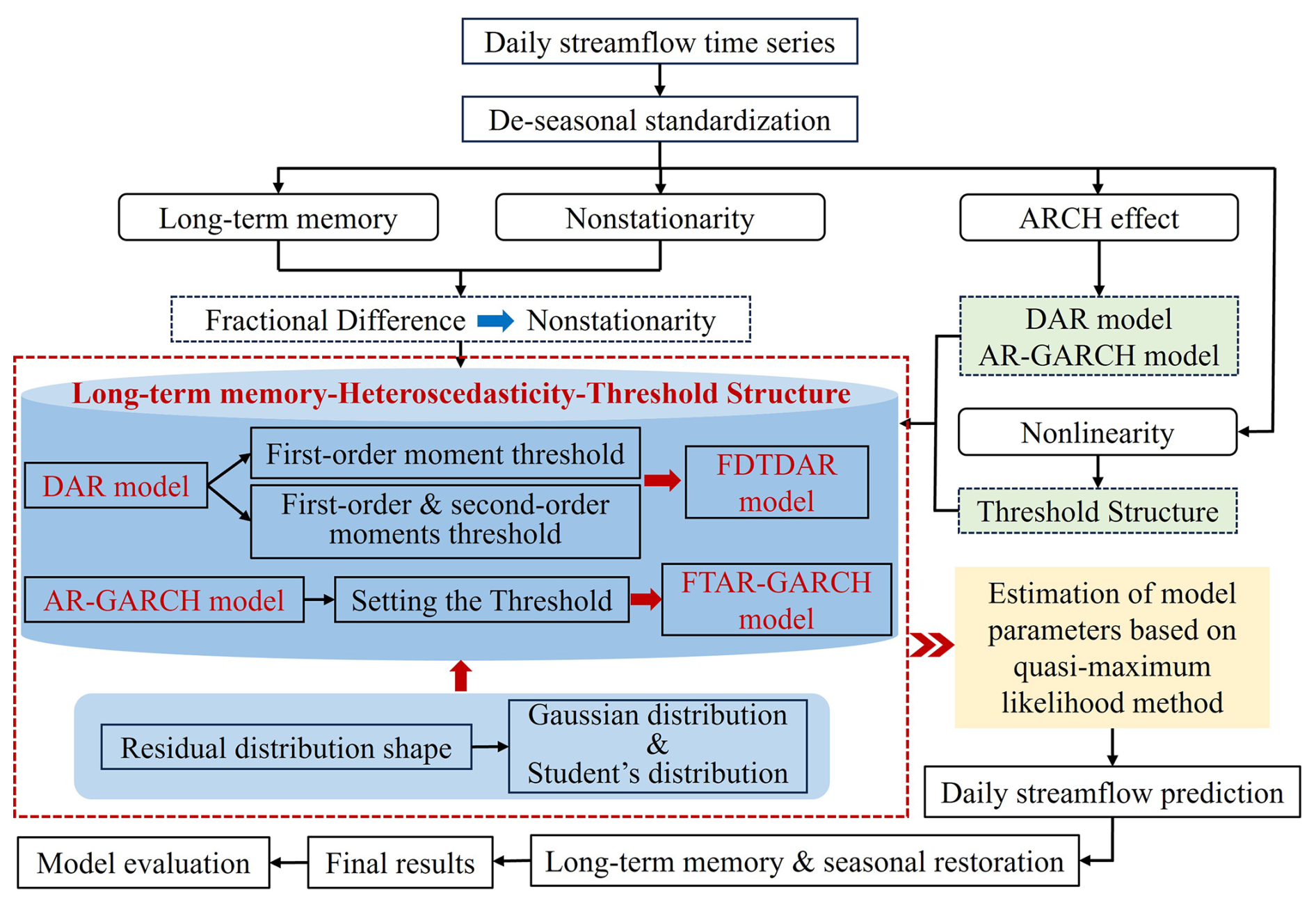
Figure 3 Methodological workflow of the Fractional-differenced dual-threshold double autoregressive (FDTDAR) framework for non-linear and long-memory streamflow prediction.

The residual diagnostics of the model are conducted using the autocorrelation function (ACF), by examining whether the residual autocorrelations at various lag times fall within the 95 % confidence interval around 0. If ACF values lie within this interval, the residuals can be considered approximately white noise, indicating that the model has effectively captured the variation structure of the time series.

An overview of the process of building the model in this study is shown in Fig. 3.

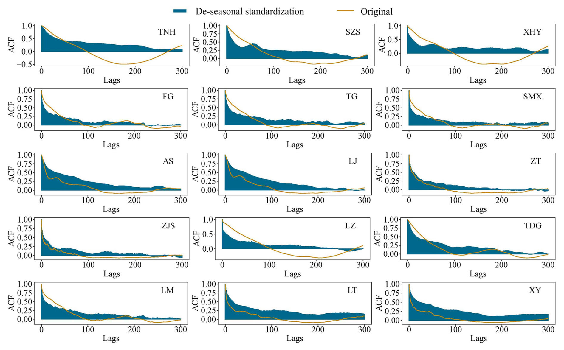
Figure 4 Autocorrelation coefficient (ACF) for original and de-seasonal standarded daily streamflow time series in 15 stations.

4 Results

4.1 Statistical diagnostics and model selection rationale

The results of various diagnostic tests on the daily streamflow time series are presented in Figs. 4, S2, and Tables S1–S3 in the Supplement. The ACF (Fig. 4) and the Hurst exponent results (Table S1) indicate that the daily streamflow series exhibits long-term memory characteristics, and that seasonality weakens the strength of this memory. The results of the 3 unit root tests (Table S2) reveal that the series is non-stationary. Considering its long-memory properties, fractional differencing was adopted to achieve stationarity, which satisfied the model assumptions. The LM test yields consistent results (Table S4). The nonlinearity test results (Table S3) suggest that the daily streamflow time series exhibits significant nonlinear behavior, implying that the model structure in this study should be modified to accommodate nonlinear dynamics.

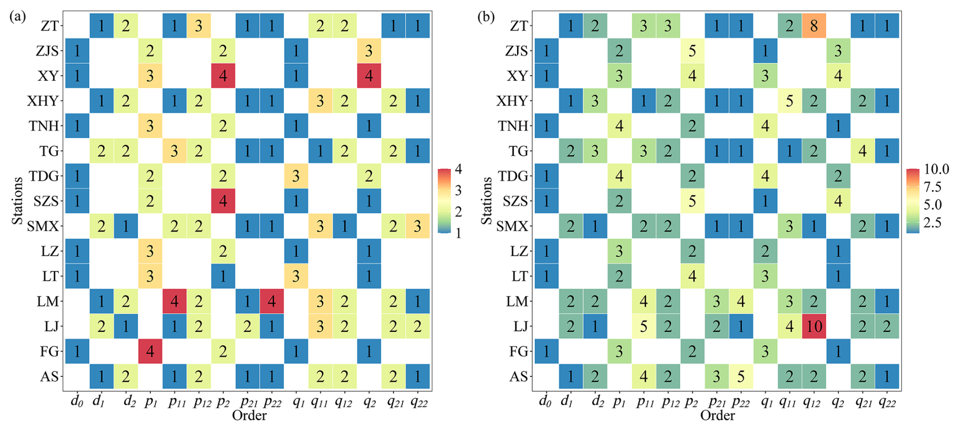
Figure 5 The order of the FDTDAR model for 15 hydrological stations, where (a) and (b) represent the normal distribution and the Student's t distribution, respectively.

The diagnostic results presented above provide critical insights into the statistical characteristics of the daily streamflow time series, including long-term memory, non-stationarity, heteroscedasticity, and nonlinearity. These findings form a solid foundation for selecting appropriate modeling strategies in the subsequent sections. Specifically, the detection of long-term memory and non-stationarity justifies the use of fractional differencing methods to ensure model validity. The presence of ARCH effects highlights the need for models capable of capturing time-varying volatility, while the identified nonlinear dynamics suggest that linear structural models may be insufficient. DAR-type models have emerged as strong competitors to the widely used heteroscedastic GARCH models, due to their simple mathematical formulation, ease of parameter estimation, and ability to accurately characterize real-world data. Based on the results of this section, the next section introduces an enhanced modeling framework (FDTDAR model) based on the DAR family, which integrates long-memory components, heteroscedasticity, and nonlinear dynamics to better capture the complex behavior of daily streamflow.

Figure 5 illustrates the presence of the FDTDAR model at various hydrological stations. In the FDTDAR models with equal lag times (Eq. 9), the value of d₀ is consistently 1, while in another form (Eq. 8), the lag times (d₁ and d₂) have values of 1 to 3. Furthermore, the order of FDTDAR-n and FDTDAR-t models generally ranges from 1 to 5 d, except for ZT and LJ stations, where the FDTDAR-t model order reaches 8 and 10.

Due to intensified climate change and enhanced human activities, the nonlinearity of daily streamflow time series may continue to strengthen. FDTDAR models with the same lag time essentially use a threshold at the mean level to simultaneously constrain the behavior of the first and second moments, which may be challenging in addressing the challenges brought about by nonlinear changes at the second-moment level in daily streamflow time series. Except for ZT and LJ stations, the complexity of the FDTDAR models under the two residual distribution forms is generally consistent.

The thresholds for the FDTDAR model with different residual distributions at 15 hydrological stations are presented in Table 2. The inputs for each model are daily streamflow time series that have undergone seasonal standardization and fractional differencing. The thresholds for the FDTDAR models based on two residual distributions are identical for the XHY, ZT, LZ, LM, LT and XY hydrological stations.

Table 2 Thresholds of the FDTDAR model in 15 hydrological stations, where n and t represent normal and Student's t distributions, respectively. r1, r2 and r0 are the thresholds for classifying streamflow into different flow regimes, where r1 and r2 are derived from Eq. (8) and r0 is derived from Eq. (9).

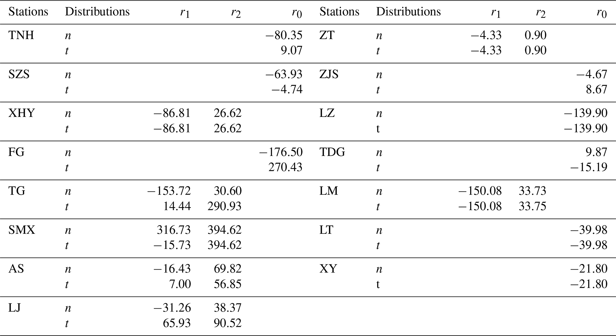
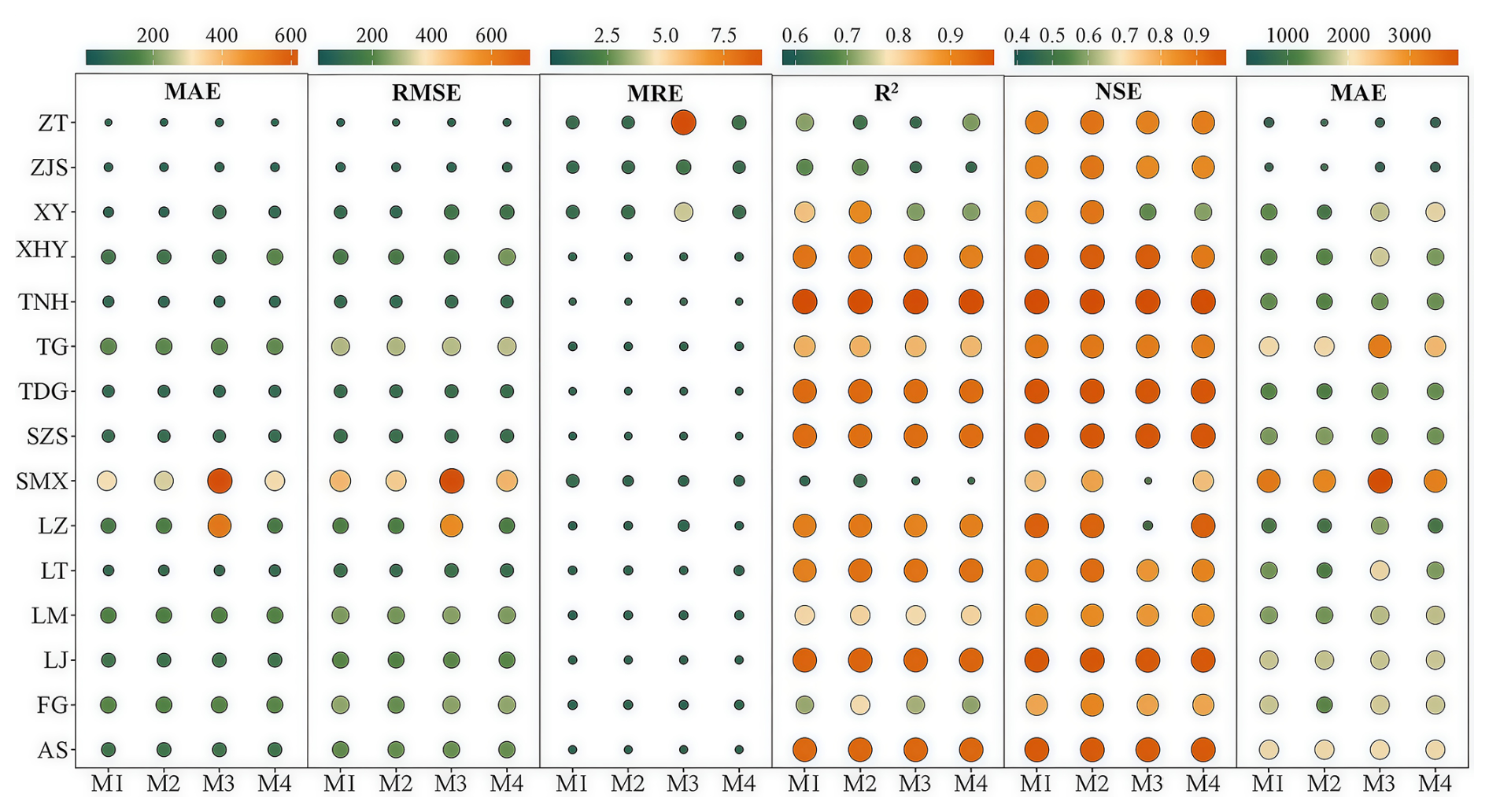
Figure 6 Prediction evaluation indicators of long memory threshold models, where M1, M2, M3 and M4 are FDTDAR-n, FDTDAR-t, FTAR-GARCH-n and FTAR-GARCH-t models, respectively.

4.2 Comparison between FDTDAR and FTAR-GARCH models

Figure 6 compares the predictive performance of various long memory threshold models for 15 hydrological stations. For mainstream hydrological stations, higher levels of average error (MAE and MRE) and extreme error (RMSE and AME), and lower R2 and NSE values, indicate poor predictive accuracy for the four models at the SMX station. For the vast majority of stations, the R² and NSE values of both FDTDAR and FTAR-GARCH models exceed 0.8, but the FDTDAR model yields smaller MAE and RMSE values. In addition, the shape of the residual distribution exerts a certain influence on predictive performance, with models based on the Student's t distribution exhibiting smaller error metrics and larger R² and NSE values. Overall, compared with the FTAR-GARCH model, the FDTDAR model demonstrates superior predictive capability, and the Student's t distribution is more suitable than the normal distribution for characterizing the variability of daily streamflow.

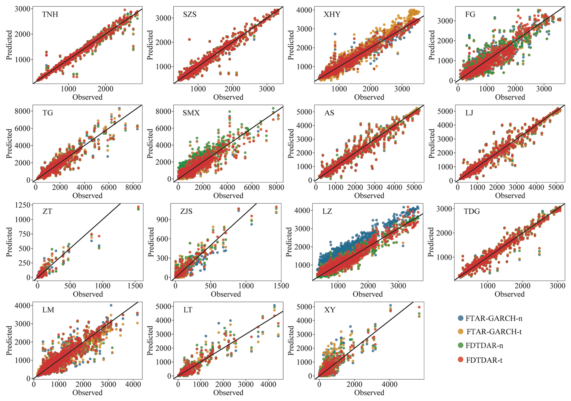
Figure 7 Scatter plots of observed versus predicted daily streamflow for the 15 stations during the testing period. Colors represent different model variants (FTAR-GARCH-n, FTAR-GARCH-t, FDTDAR-n, and FDTDAR-t).

Furthermore, Fig. 6 illustrates that, in the case of four tributary hydrological stations (ZT, ZJS, LT, and XY), the FDTDAR type models exhibit relatively lower values of MAE, RMSE, MRE, and AME, while simultaneously having higher R² and NSE values compared to FTAR-GARCH models. The predictive results of FDTDAR and FTAR-GARCH models vary under different distribution assumptions, with the t-distribution yielding superior predictive performance. In short, FDTDAR models demonstrated outstanding predictive capabilities in the daily streamflow time series at tributary hydrological stations, and the t-distribution significantly improved the accuracy of model predictions.

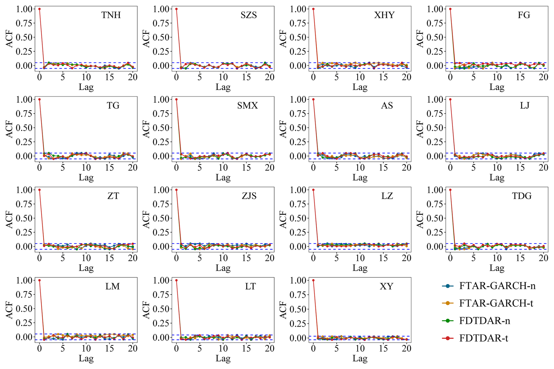
Figure 8 Autocorrelation function (ACF) plots of the standardized residuals for the 15 gauging stations during the testing period. The subplots compare the residual series derived from the FTAR-GARCH-n, FTAR-GARCH-t, FDTDAR-n, and FDTDAR-t models. The horizontal blue dashed lines represent the 95 % confidence intervals. The decay of ACF values to within these significance bounds across all stations indicates that the model residuals are largely uncorrelated, approximating a white noise process.

Predictive performance of the FDTDAR-n, FDTDAR-t, FTAR-GARCH-n, and FTAR-GARCH-t models at 15 hydrological stations reveals that, for the majority of stations, the degree of clustering of predicted points around the 1:1 line is stronger for the FDTDAR models compared to the FTAR-GARCH models (Fig. 7). Under the assumption of the Student's t distribution, both FDTDAR and FTAR-GARCH models exhibit better matching with observed daily streamflow compared to their counterparts assuming normal distribution (FDTDAR-n and FTAR-GARCH-n models). This suggests that the FDTDAR models have stronger predictive capabilities for daily streamflow time series compared to the FTAR-GARCH models, and the student's t distribution improves the predictive performance and peak description ability of the models under the classical normal distribution assumption.

Figure 8 shows that the ACF of the residual series from the long memory threshold FDTDAR and FTAR-GARCH models, based on two different residual distributions, are within the confidence intervals, indicating the absence of autocorrelation in the residual series. This implies that both model types effectively capture practical information in the daily streamflow time series, and the model predictions are reliable.

4.3 Effectiveness evaluation of long memory threshold structure

This section compares the prediction performance of DAR-type and AR-GARCH-type models under three different structures (integer differencing, long memory, and long memory threshold) and two residual distribution assumptions. In the point prediction comparison, R² and NSE values are chosen to assess the prediction accuracy of the model. The DM test is employed to identify the optimal prediction model structure and type for each station.

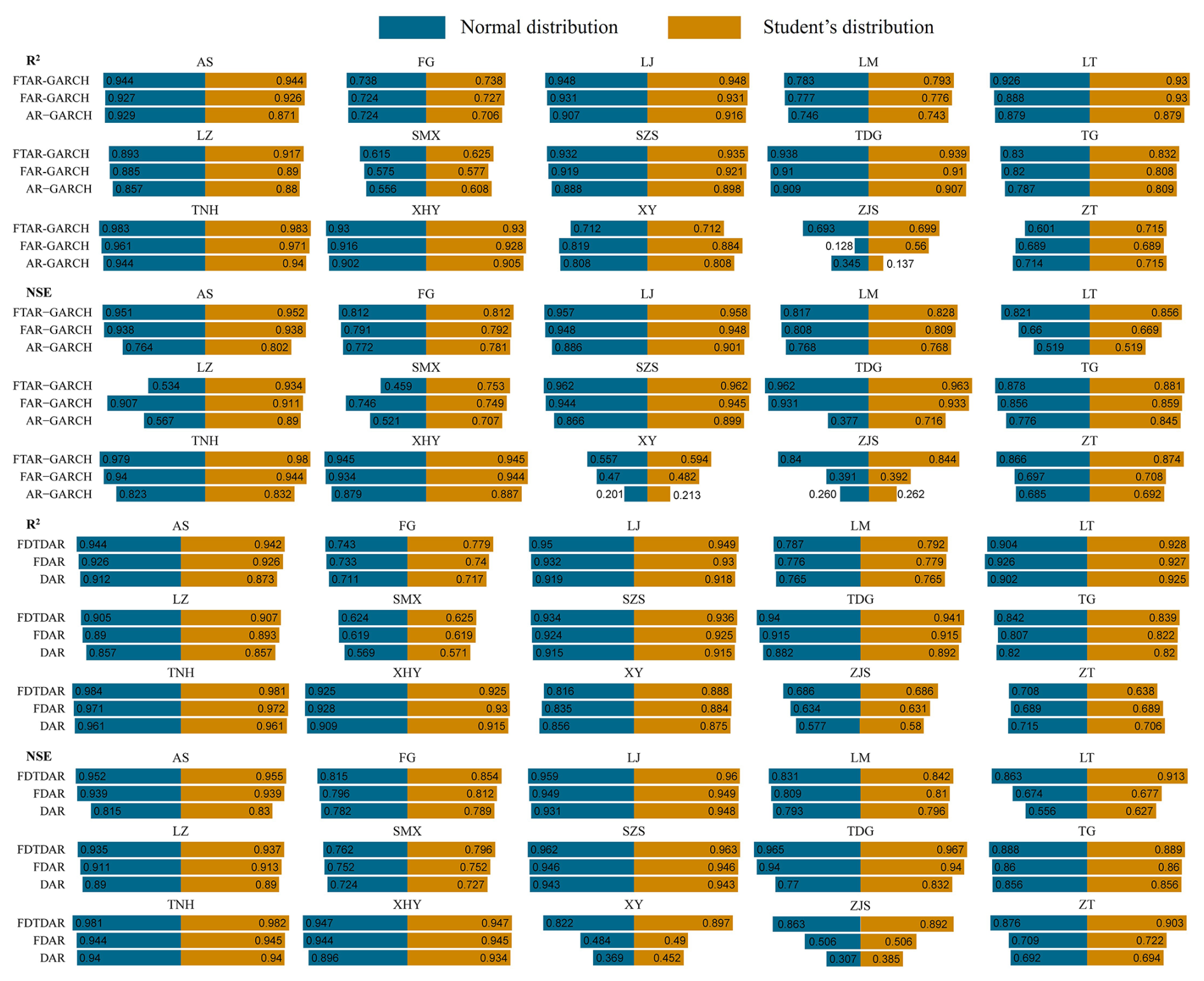
Figure 9 Comparison of prediction accuracy for DAR-type and AR-GARCH-type models based on three structures with two residual distributions at 15 stations. (Integer difference structure: AR-GARCH and DAR; Long memory structure: FAR-GARCH and FDACR; Long memory threshold structure: FTAR-GARCH and FDTDAR).

Figure 9 reveals that, at most stations, under the “long memory threshold” structure that considers nonlinear changes, both AR-GARCH-type and DAR-type models exhibit higher R² and NSE values than the two linear structures. Furthermore, the FAR-GARCH and FDAR models, which account for long-term memory, significantly improve the NSE values of the classical AR-GARCH and DAR models based on integer differencing. This indicates that the long-term memory and strong nonlinearity in the daily streamflow time series significantly influence the predictive performance of the models, and the long memory threshold structure is effective in improving the accuracy of daily streamflow predictions.

The comprehensive evaluation results of the predictive performance of DAR-type and AR-GARCH-type models under different structures are presented in Table 3. In the group of Linear vs. Nonlinear, the linear models are derived from the advantageous models in the difference group, while the two superior models in the residual distribution comparison groups come from the optimal models of each distribution. It can be observed that, except for the ZJS station, the long memory structure based on fractional differencing effectively enhances the predictive ability of the two type models under traditional integer differencing. The p-values less than 0.05 indicate that the long-memory threshold structure significantly contributes to improving the prediction accuracy of the two type models (DAR and AR-GARCH) with linear changing characteristics (excluding the ZJS station). Additionally, the results of different residual comparison group indicate that XHY, FG, TG, SMX, AS, and TDG stations are more suitable for the t-distribution in DAR-type model, while in AR-GARCH-type, SZS, XHY, TG, AS, ZT, ZJS and LT stations exhibit this preference.

Table 3 p-value of DM test for DAR-type and AR-GARCH-type models under different structures (M1 vs. M2 shows that the original hypothesis of the DM test is that the prediction performance of M1 is better than M2).

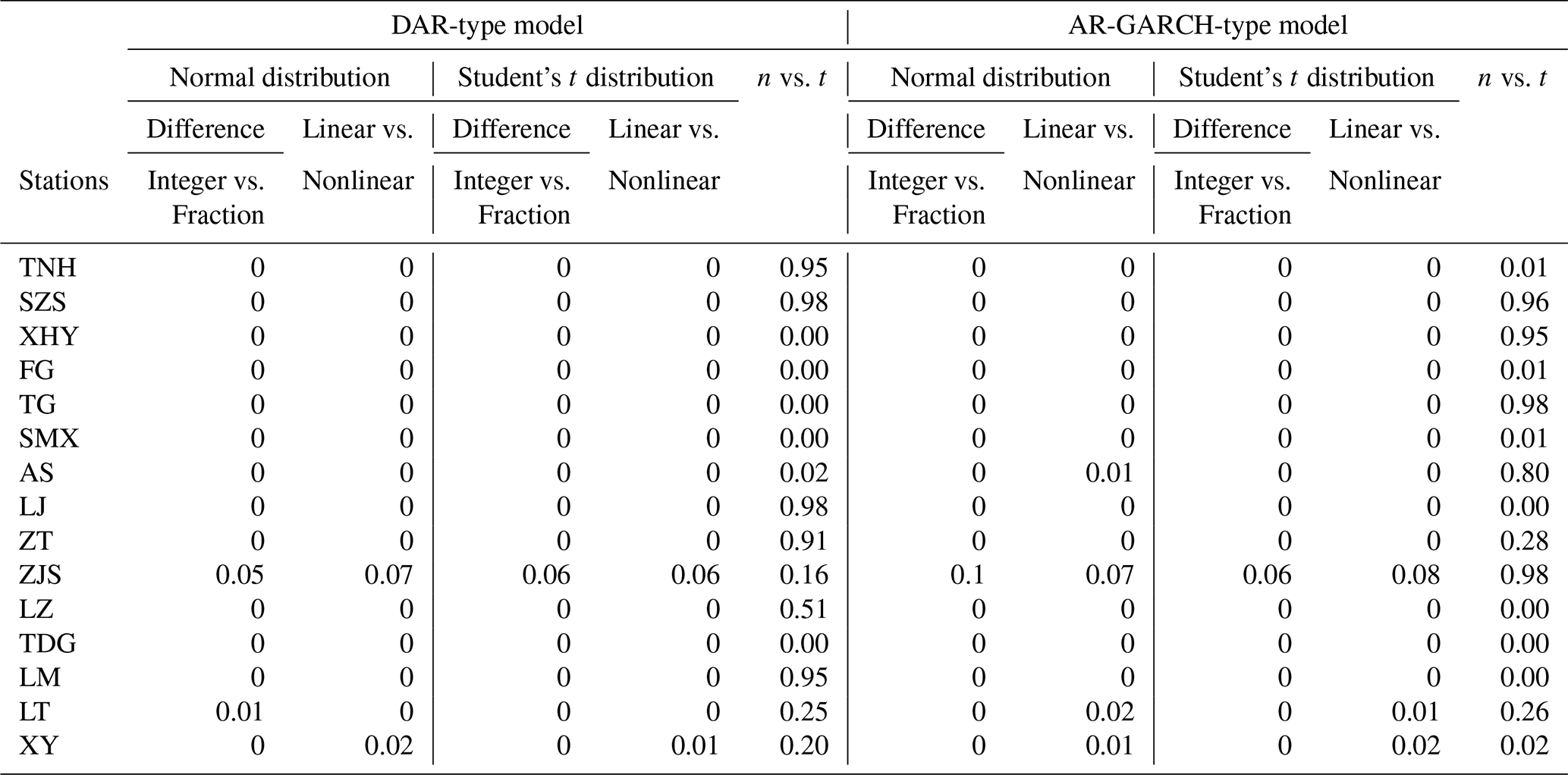
Further comparison was conducted on the preferred models of the two types at each station, with the null hypothesis (DM hypothesis) set as DAR-type model being superior to AR-GARCH-type. The optimal models for each station were ultimately determined, with XHY, FG, TG, SMX, AS, and TDG stations favouring the FDTDAR-t model, the DAR-n model performing well at the ZJS station, and the remaining stations adopting the FDTDAR-n model.

5 Discussions

5.1 Properties of daily streamflow time series

The daily streamflow time series is influenced by natural and human factors, presenting seasonality, long-term persistence, non-stationarity, and time-varying volatility (ARCH effect), which play a crucial role in simulation and prediction. However, the long-term persistence has been overlooked in most studies. The integer difference method is often used to address non-stationary issues to smooth the series (Myronidis et al., 2018; Yan et al., 2022), but it also eliminates the long-term memory information of daily streamflow, resulting in incomplete input information for the model and affecting the simulation and prediction accuracy. Some scholars (Mehdizadeh et al., 2019; O'Connell et al., 2016; Yang and Bowling, 2014) have also studied long-term persistence, demonstrating its importance in predicting the daily streamflow process. However, those researchers have not conducted the second-order moment components, making it impossible to prove whether the ARCH effect is related to long-term persistence. In recent years, an increasing number of researchers (Dimitriadis et al., 2021; Graves et al., 2017; Grimaldi, 2004) have reported that the detected ARCH effect in the classic AR model may be suspicious due to the lack of consideration of long-term memory, and the results of the further constructed time-varying fluctuation model are thought-provoking. This implies that the results obtained in existing studies on daily streamflow prediction by time series models may be biased due to an incomplete understanding of the characteristics of the research targets. Given the existing problems in the research, in addition to the seasonality and non-stationarity of the daily streamflow time series, this study also considers long-term persistence and time-varying volatility, which improved the prediction accuracy while ensuring the correctness of the ARCH effect.

In addition, time irreversibility is also an important property of streamflow time series, although it is negligible in other hydrological cycle components (e.g., precipitation, evapotranspiration) (Vavoulogiannis et al., 2021). Stationary processes in statistics are typically reversible over time, but the nonlinearity of underlying dynamic procedures is reflected in time irreversibility. River dynamics argues that the time irreversibility of streamflow sequences mainly depends on various triggering factors in the formation process and exhibits nonlinear changes. Specifically, the increase in streamflow is largely determined by short-term meteorological drivers, which are inherently the dynamic characteristics of precipitation, while groundwater dynamics respond to the streamflow reduction process (Serinaldi and Kilsby, 2016). Table S3 provides clear evidence of the nonlinear nature of daily streamflow, supporting the existence of time irreversibility. Threshold regression models such as TAR-GARCH and DTDAR have been successful in catching the nonlinear characteristics of daily streamflow time series, and numerous studies have confirmed their effectiveness in solving nonlinear problems. Therefore, the modeling approach used in this study, incorporating long memory, thresholds, and time-varying fluctuations, is more suitable for describing daily streamflow time series.

5.2 DAR-type models vs. AR-GARCH-type models

From the general situation of the model, both the DAR and the AR-GARCH models can grasp the first- and second-order moment information of the daily streamflow time series, but the DAR model has a simpler structure. One of the most significant differences between these models is that the second-order moment description of the GARCH model uses past conditional fluctuations, as well as past daily streamflow information, to estimate the current conditional variance. In contrast, the DAR model relies solely on past streamflow information. Previous period streamflow values and conditional fluctuations reflect the fluctuation aggregation and long-term behavior characteristics of the time series, respectively. Nevertheless, most of the literature (Guo et al., 2021b; Modarres and Ouarda, 2013; Pandey et al., 2019) indicated that the classic GARCH model is insufficient in describing fluctuation aggregation effect, which significantly exists in hydrological time series (Fig. S1). Moreover, limited data availability in practice means that short-term volatility clustering is often prioritized over long-term volatility. To avoid long-term persistent interference, the daily streamflow time series is processed with an effective fractional difference approach before being used as the model input. Taken together, these constraints result in better prediction performance and accuracy for the DAR-type models than for the AR-GARCH-type models.

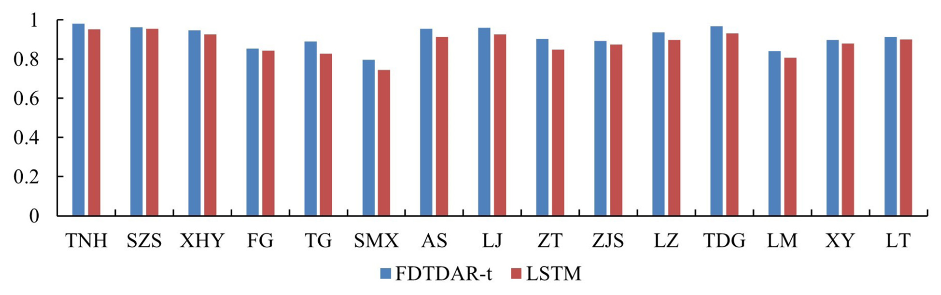
Figure 10 Comparison of prediction accuracy (NSE) during the validation period between LSTM and FDTDAR-t models.

5.3 Threshold regression models

Geosciences acknowledge that data are the only reliable source of information for model construction, derivation, and prediction. The concepts of stationarity and non-stationarity are considered modeling options rather than properties of data because stochastic models are inherently mathematical constructs (Dimitriadis and Koutsoyiannis, 2018; Koutsoyiannis and Montanari, 2015). However, model properties such as randomness, determinism, stationarity, and non-stationarity should always align with the data. Furthermore, stationarity is ergodic in practice, i.e., the selected sample data is representative of the entire stochastic process (Koutsoyiannis and Montanari, 2015). Meanwhile, the short-term behavior of hydrological predictions can allow model structure to be inferred from sample data. These provide evidence for the rationality of using data to build models and predict in this study. In regression analysis, the stability of coefficient estimates is usually studied, but the external force disturbance that causes structural breaks in the streamflow time series cannot be avoided, which hinders the applicability of ordinary linear regression models.

Affected by multiple factors such as global climate change and intense human activities, the nonlinearity of the basin hydrological system has been enhanced. As early as the 1990s, Xia et al. (1997) had conducted in-depth and systematic research on nonlinear hydrological systems, and explored the nonlinear process of streamflow generation and transformation, as well as the nonlinear mechanism of streamflow formation and transformation from response units to watershed scales. He further proposed a new nonlinear model for streamflow simulation and prediction. In practice, the hydrological gain of streamflow magnitude generated by precipitation is closely related to highly nonlinear controlling factors (such as precipitation, underlying surface conditions, soil moisture, etc.), resulting in the system gain of streamflow generated by precipitation being non-steady, which is a nonlinear relationship. Therefore, linear mechanism process analysis is difficult to meet the needs of basin streamflow simulation and prediction.

In view of the nonlinear changes in water resource systems (Wu et al., 2023), a series of multivariate analysis methods based on nonlinear relationships have been developed, where numerous conditioning factors are input into models to simulate streamflow (Song et al., 2022). These methods improve the simulation and prediction accuracy by comprehensively considering the influence of climate factors, soil properties, terrain conditions and vegetation types on streamflow (Tiwari et al., 2022). Regarding the land surface water balance, precipitation reaches the ground after being intercepted by vegetation leaves, and infiltrates through the soil or becomes surface streamflow. The water intercepted by the leaves and a portion of the water in the soil returns to the atmosphere through evaporation, and the soil moisture absorbed by vegetation for growth is transpired through the leaves, ultimately forming the cycle of atmospheric-land surface water. At present, coupled process and data-driven multivariate models are developing rapidly, which can take into account the mechanisms of streamflow and further enhance the simulation and prediction accuracy of single-type models (Zhong et al., 2023).

The univariate method constructed in this study is based on various performance characteristics of streamflow time series, reducing the uncertainty of input factors by generalizing the rainfall-runoff process in the basin, making practical applications more convenient. The threshold concept is used to explain the nonlinear variations in the series, which can more accurately describe the linear variation process of daily streamflow time series within different threshold intervals, and has strong robustness and applicability. Moreover, the threshold model is effective in capturing the asymmetric effects of rising and falling changes in daily streamflow time series, offering higher flexibility in grasping variation information compared to linear structure models, with high potential for simulation and prediction.

5.4 Limitations of FDTDAR models

The DAR-type models offer a simpler and more interpretable approach to time series modeling. They are particularly advantageous in scenarios where domain interpretability, limited sample sizes, and computational efficiency are critical. Their transparent structure facilitates parameter estimation, theoretical analysis, and diagnostic evaluation, making them especially suitable for hydrological applications that typically involve noisy data, sparse observations, and operational constraints, thereby enhancing their robustness and reliability in real-world application (Li et al., 2019; Ling, 2007).

However, the proposed FDTDAR model also has inherent limitations. First, although it can effectively capture regime-switching behavior and certain nonlinear dynamics, it may fall short in modeling the complex and high-dimensional variations commonly present in large-scale hydrological or climate datasets. Second, the modeling capacity of the FDTDAR framework is constrained by the number of thresholds and lag terms that can be practically specified, which limits its structural flexibility compared with more adaptive, data-driven models such as LSTM. Third, the prediction performance of FDTDAR models often depends heavily on the correct setting of thresholds and lag structures. This adjustment process can be challenging in practice and often requires expert domain knowledge or a large number of traversal trials, which may reduce the generalization ability of the model across different regions or datasets.

In contrast, machine learning models, particularly deep learning approaches, can learn complex patterns, nonlinearities, and long-term dependencies directly from the data without strong prior assumptions about model structure (van Cranenburgh et al., 2022). Figure 10 shows that the prediction accuracy of the FDTDAR-t model is comparable to, or even slightly higher than, that of the LSTM model. These models often demonstrate outstanding predictive performance in many benchmark tasks. However, their “black-box” nature raises concerns about interpretability and transparency, which are critical in scientific and decision-making contexts such as hydrology (Beven, 2020; Hosseini et al., 2025). In addition, the high computational cost, demand for large training datasets, and sensitivity to hyperparameter tuning may restrict their applicability in resource-limited environments or real-time forecasting systems.

Given these trade-offs, this study focuses on DAR-type models as a theoretically grounded and operationally tractable alternative to traditional AR-GARCH models. While the proposed FDTDAR framework strikes a balance between model simplicity and nonlinear expressiveness, we acknowledge that future research should include comprehensive comparisons with state-of-the-art machine learning models. Such efforts would help further assess the strengths and limitations of the proposed approach and explore the potential of hybrid frameworks that combine the interpretability of statistical models with the flexibility of machine learning techniques.

In terms of the model residuals, although the Student's t distribution used in this study effectively captures heavy tails, it does not account for potential asymmetry in the distribution of hydrological residuals. In real-world streamflow processes, especially during flood or drought events, residuals may exhibit skewness in addition to heavy tails. Therefore, more flexible distributions, such as the skewed or generalized t-distributions, may offer a better fit for such cases. While these distributions were not explored in the present study, they represent a promising direction for future research aimed at enhancing the model's adaptability to extreme or asymmetric behavior.

6 Conclusions

The nonlinear changes of the daily streamflow time series driven by the external environment cannot be ignored, and the strong non-stationarity and volatility, as well as its long-term memory, together lead to an increase in the difficulty of streamflow prediction, which brings great challenges to the traditional time series models. To address this issue, this study introduced a novel DAR model and further proposed the FDTDAR model, which considered these critical features and added a threshold for improving the accuracy of daily streamflow time series prediction. The main conclusions of this study can be summarized as follows:

1. The DAR model is a better alternative to the AR-GARCH model for predicting daily streamflow time series. Both the linear structure DAR and the threshold FDTDAR models outperform the AR-GARCH, TAR-GARCH, and LSTM models in terms of predictive ability.

2. The nonlinear changes of the daily streamflow time series are reflected in multiple linear structures by adding the threshold, improving the accuracy of the single linear structure method. The NSE values of the FDTDAR and TAR-GARCH models are higher than those of the DAR and AR-GARCH models by 0.013–0.556 and 0.031–0.582, respectively.

3. The hypothesis type based on the t-distribution for residuals stands out in the prediction of daily streamflow time series for both FDTDAR and FTAR-GARCH models and is a better choice than the traditional normal distribution.