Novel insights into deep groundwater exploration by geophysical estimation of hard rock permeability

Deep groundwater exploration in hard rock terrains is critical in regions where deep aquifers may offer long-term water security amidst an increasing scarcity. However, such exploration is globally challenged by geological complexity and the limitations of traditional investigative techniques. Accurate estimation of hydraulic parameters, particularly permeability (k), is essential for effective groundwater management and future resource planning. Conventional borehole-based methods for measuring k are invasive, costly, time-consuming, and limited to sparse, point-scale observations, making them inadequate for characterizing deep and heterogeneous aquifer systems. Geophysical methods offer a promising non-invasive alternative, enabling broader spatial coverage with reduced surface disturbance. Previous empirical geophysical approaches, such as vertical electrical sounding (VES), are generally restricted to shallow depths (< 200 m), relatively homogeneous geological settings, and one-dimensional interpretations. This study demonstrates, for the first time, the use of controlled-source audio-frequency magnetotellurics (CSAMT) to estimate two- and three-dimensional k distributions to depths exceeding 1 km in crystalline and sedimentary terrains. The method relies on an empirical resistivity–permeability relationship calibrated using 116 core samples from six boreholes (0–200 m). While the specific equation derived in this study is site-specific to the Jinji area and should not be directly transferred elsewhere, the broader methodology, integrating CSAMT resistivity with local borehole calibration, offers a transferable framework for k estimation in other complex geological settings. The results show that CSAMT, when calibrated with borehole data, can reliably capture deep subsurface variability and produce spatially continuous hydrogeological models in hard rock terrains. While CSAMT inversion is inherently ill-posed, the incorporation of ground-truth data significantly enhances model robustness and interpretability. By reducing dependence on extensive drilling, this approach represents a significant advancement in deep groundwater exploration. It provides a scalable methodology for sustainable groundwater resource management, while emphasizing the need for local calibration in any new application.

1 Introduction

Metamorphic and igneous rocks dominate Earth's crust and cover about one-third of its surface (Amiotte Suchet et al., 2003). In hard rock terrains, groundwater research focuses on delineating subsurface structures, such as faults and fractures that control water storage and flow (Fernando and Pacheco, 2015; Hasan et al., 2021). A key parameter in this context is aquifer potential, which reflects the capacity of rock formations to store and transmit groundwater and is influenced by lithology, structural complexity, mineral composition, weathering, and infiltration depth (Majumdar and Das, 2011; Zhu et al., 2017). However, accurately characterizing the lateral and vertical heterogeneity of these properties remains challenging due to limited data and the complexity of massive rock units (Dewandel et al., 2006). In such settings, conventional methods often fall short, leading to inefficient or unsustainable groundwater development (Nwosu et al., 2013; Worthington et al., 2016). Developing cost-effective and reliable approaches for subsurface assessment is therefore essential for managing groundwater in hard rock environments.

Groundwater at depths beyond 500 m is typically isolated from surface hydrological influences and often exhibits brackish or saline characteristics (Ferguson et al., 2023). Its strategic importance is increasingly recognized, particularly in geologically- and environmentally-constrained settings (Gleeson et al., 2014). In the Jinji region, several factors necessitate focused investigation of deep aquifers. Surface water is scarce and unreliable, while the shallow subsurface is dominated by fresh granite, which has inherently low porosity and permeability, limiting groundwater availability. By contrast, deeper fractured zones in granite, sandstone, and hornstone present more favorable hydrogeological conditions. Recent national water initiatives in China have emphasized deep subsurface exploration in structurally complex terrains to identify underutilized aquifers for enhancing long-term water security. Comprehensive assessment of these deep reserves is essential to evaluate their recharge potential and integrate them into sustainable resource management strategies (Condon et al., 2020; Hasan and Shang, 2022). As pressure on surface and shallow groundwater intensifies, deep aquifers may serve as a vital buffer against increasing environmental and socio-economic stress.

Multiple studies have documented the rapid depletion of global groundwater reserves, raising serious concerns about long-term water sustainability (Wada et al., 2010; Laghari et al., 2012; Jasechko et al., 2024). Addressing this challenge requires accurate and detailed assessments of groundwater resources, which depend critically on a clear understanding of subsurface hydraulic properties. Permeability (k) is a key parameter that describes the ease with which fluids can move through a porous medium, while the capacity to store water is more directly characterized by porosity. This parameter is crucial for aquifer analysis in various hydrogeological settings (Allègre et al., 2016; Esmaeilpour et al., 2023; Carbillet et al., 2024). Borehole testing remains the standard method for estimating k and related aquifer parameters (Niwas and De Lima, 2003; Hasan et al., 2021). However, borehole investigations are often limited by high costs, logistical challenges, and poor spatial coverage, particularly in rugged terrains, while offering only localized information with limited ability to image lateral and deep structures (Singh, 2005; Fiandaca et al., 2018). These limitations contribute to uncertainties in groundwater assessments, especially in data-scarce regions (Hasan and Shang, 2022). Alternatively, it is essential to develop methods that minimize reliance on costly drilling while still enabling reliable estimation of permeability within prospective rock formations.

Table 1 Comparative overview of geophysical methods for hydrogeological investigations.

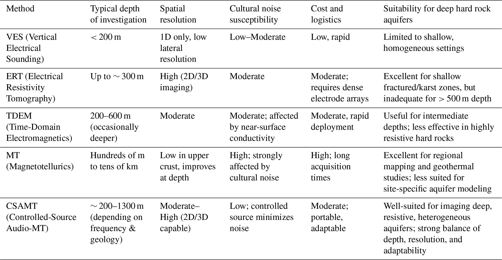
Geophysical methods are widely and effectively employed to enhance subsurface characterization in groundwater studies (Daily et al., 1992; Jardani et al., 2007; Hinnell et al., 2010; Fu et al., 2013; Jiang et al., 2014; Kouadio et al., 2023). Compared to conventional drilling, these techniques offer significant advantages in cost, deployment speed, environmental impact, and spatial extent (Hu et al., 2013; Fusheng et al., 2022). Their ability to image subsurface variations in both vertical and lateral dimensions makes them particularly effective in heterogeneous terrains (Hasan et al., 2025). Among them, resistivity-based methods are widely used due to their sensitivity to lithology, porosity, fractures, and fluid content (Hasan et al., 2021; Asfahani, 2023). Common techniques include electrical resistivity tomography (ERT), vertical electrical sounding (VES), and electromagnetic methods such as magnetotellurics (MT), time-domain electromagnetics (TDEM), and controlled-source audio-frequency magnetotellurics (CSAMT) (Soupios et al., 2007; Bauer-Gottwein et al., 2010; Pollock and Cirpka, 2012; Jiang et al., 2014; Di et al., 2020). A comparative summary of these methods (Table 1) highlights their relative strengths and limitations in terms of penetration depth, spatial resolution, sensitivity to cultural noise, and cost. VES is cost-effective but limited to shallow one-dimensional profiling (< 200 m) (Niwas and De Lima, 2003; Majumdar and Das, 2011). ERT improves resolution and enables 2D/3D imaging up to ∼ 300 m but requires intensive fieldwork and is less effective in extreme resistivity environments (Abbas et al., 2022; Hasan and Shang, 2022). For deeper targets, electromagnetic methods such as TDEM, MT, and CSAMT are often employed (Bauer-Gottwein et al., 2010; Di et al., 2020; Gonzalez-Duque et al., 2024). MT achieves the greatest penetration depth (up to tens of kilometers) but often sacrifices resolution in the upper crust and is highly susceptible to cultural noise (Simpson and Bahr, 2005). TDEM provides rapid deployment and intermediate depth coverage (hundreds of meters) but suffers reduced sensitivity in resistive hard rock (Bauer-Gottwein et al., 2010). By contrast, CSAMT bridges these approaches: with a controlled source and frequency tuning, it achieves intermediate-to-deep penetration (> 1000 m) with improved resolution in resistive hard rock settings and strong immunity to cultural noise (Smith and Booker, 1991; Zonge and Hughes, 1991; Wang et al., 2015; Zhang et al., 2021). The choice between resistivity and electromagnetic techniques is contingent upon parameters like investigation depth, resolution requirements, geological complexity, and logistical constraints (Majumdar and Das, 2011; Hasan et al., 2025). Given the objectives of this study, to characterize deep fractured aquifers in crystalline and sedimentary rocks under complex geological conditions, CSAMT was selected as the most suitable technique. Its combination of penetration depth, resolution, and robustness against noise provides a practical balance between regional coverage and site-specific imaging, enabling the development of 2D and 3D permeability models that are otherwise difficult to achieve with alternative methods.

In fractured rocks like granite, metamorphic, and sandstone formations, fluid flow is largely controlled by fracture networks rather than matrix porosity. Accurate hydraulic assessment in such settings benefits from integrated geophysical and hydrogeological approaches to better capture spatial variability and improve flow modeling (Hasan et al., 2021; Abbas et al., 2022). Resistivity-based techniques are particularly valuable for delineating subsurface structures and identifying water-bearing zones. Because electrical resistivity is sensitive to porosity, saturation, fracture density, and fluid salinity, it is increasingly used to infer k in heterogeneous geological settings (Mudunuru et al., 2022; Yan et al., 2024). Permeability is influenced by numerous parameters, including porosity, fracture density and orientation, grain size distribution, degree of weathering, pore connectivity, and saturation level, highlighting the utility of resistivity measurements as indicators for evaluating groundwater flow potential (Gerke et al., 2011; Worthington et al., 2016; Pellet et al., 2024).

Empirical and semi-empirical models have been developed to estimate hydraulic properties from geophysical measurements, particularly in data-sparse regions (Niwas and De Lima, 2003; Singh, 2005; Soupios et al., 2007; Hasan et al., 2021; Asfahani, 2023). In parallel, resistivity-based methods and hydrogeophysical inversion techniques have been developed to more rigorously estimate hydraulic parameters by integrating petrophysical relationships within geophysical modeling frameworks (Daily et al., 1992; Ferré et al., 2009; Binley et al., 2010; Hinnell et al., 2010; Herckenrath et al., 2012; Pollock and Cirpka, 2012; Herckenrath et al., 2013; Binley et al., 2015). These approaches have improved resolution in parameter estimation, particularly in shallow, unconsolidated, or relatively homogeneous settings. However, applications to deep, fractured, and lithologically complex environments remain limited, especially in terms of producing volumetric k models at kilometer-scale depths. Despite these advances, generation of detailed 2D and 3D k maps from resistivity data in deep, hard-rock terrains is constrained by limited borehole control, significant geological heterogeneity, and the ill-posed nature of geophysical inversion. In such contexts, integrating resistivity data with borehole measurements presents a practical, cost-effective solution for characterizing aquifer properties over large areas and depth ranges. This study builds on prior hydrogeophysical research by introducing a novel application of the CSAMT method for volumetric k modeling in a complex, fractured hard-rock setting. While previous studies have applied resistivity-based techniques to estimate hydraulic properties, this is the first to utilize CSAMT for constructing the detailed 2D and 3D k modeling beyond 1000 m depth in geologically heterogeneous terrains comprising hornstone, granite, and sandstone. Few available drilling tests were used to calibrate CSAMT-derived resistivity with laboratory-measured k, allowing the resulting empirical relationship to be applied across the broader survey domain. Several CSAMT profiles were conducted along and beyond the borehole locations, and the calibrated resistivity–permeability correlation was used to generate spatially continuous subsurface models in regions lacking direct borehole data. This integration resulted in a robust, data-constrained workflow capable of revealing k variations across diverse rock units and lithological boundaries. The method offers a practical and scalable alternative to extensive drilling campaigns, enabling a more detailed and cost-efficient evaluation of deep groundwater potential in structurally complex terrains.

Ultimately, this work extends the scope of hydrogeophysical methods by demonstrating the feasibility of applying CSAMT for deep hydraulic parameter estimation in hard rock. It bridges a critical methodological gap in hard-rock hydrogeology and sets the foundation for future CSAMT-based volumetric modeling in similarly challenging environments. This study aims to develop and apply a geophysical-based approach for mapping the spatial distribution of k in deep, hard-rock settings. By integrating CSAMT data with targeted borehole measurements, this research enhances 2D and 3D hydrogeological assessments across heterogeneous lithologies in structurally complex terrains. It also minimizes reliance on extensive drilling, demonstrating the value of non-invasive geophysical techniques as a cost-effective alternative for deep groundwater exploration.

2 Methods

This research integrates limited drilling information with geophysical data to estimate k for both 2D and 3D evaluations of groundwater resources over the entire investigated site (Fig. 1a). The main stages of the methodology are summarized in the flowchart shown in Fig. 1b.

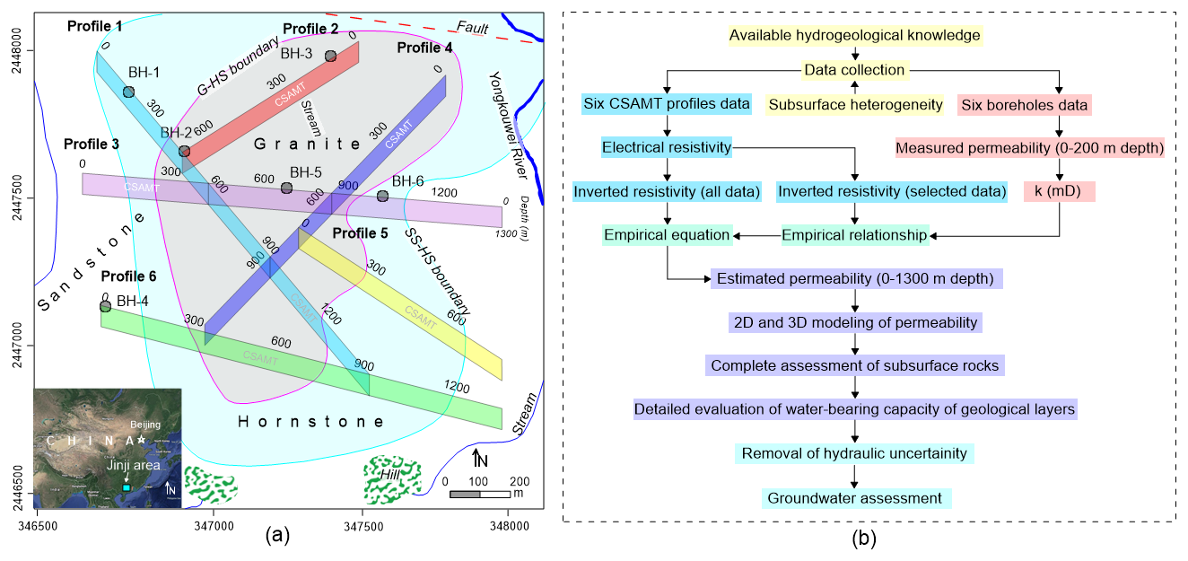
Figure 1 (a) The site map displaying six boreholes (BH-1 to BH-6) and six CSAMT survey profiles (1–6). The map also illustrates the simplified geological and hydrogeological setting, including the dominant rock types (granite, hornstone, and sandstone), the granite–hornstone (G–HS) and sandstone–hornstone (SS–HS) boundaries, major fault lines, streams, rivers, and surrounding mountainous terrain. All map layers, symbols, and annotations in panel (a) were prepared by the authors; the location inset (bottom left) uses Google Earth imagery and therefore carries the following copyright statement: “Imagery © Google; map data © Google” (Google Earth, https://earth.google.com/, last access: 28 September 2025). (b) Flowchart illustrating the methodology for generating 2D and 3D k models to enable comprehensive assessments of groundwater resources across extensive areas.

2.1 Study area and hydrogeological settings

This study is part of a national initiative in South Guangdong, China, focused on deep subsurface exploration, including groundwater resource assessment and infrastructure development such as the Jiangmen Underground Neutrino Observatory (JUNO) (Hasan et al., 2025). These actions contribute to China's national agenda toward sustainable deep-earth resource utilization. This research was conducted in the Jinji region, a geologically complex area prioritized for deep groundwater exploration (Fig. 1a). The region lies within a subtropical monsoonal climate zone, receiving ∼ 1981 mm of annual rainfall. Topography ranges from low hills to mountainous terrain (39–539.9 m elevation), with dense vegetation and varied slopes. The northern part is relatively flat, while the south includes prominent features such as the Dashishan and Qilongding Mountains. Surface drainage is primarily controlled by the Yongkouwei River in the northeast.

Geologically, the Jinji area has evolved through successive tectono-magmatic processes linked to the Yanshanian, Indosinian, and Caledonian mountain-building phases, resulting in a lithologically diverse landscape of granite, sandstone, and hornstone (Qin, 2017). Granite intrusions reflect deep crustal magmatism, while hornstone indicates contact metamorphism. Overlying Paleogene sediments record later basin development. Tectonic structuring in the area is largely influenced by the Kaiping fault-fold complex, which includes reverse, thrust, and strike-slip faults formed under prolonged crustal compression and later modified by strike-slip tectonics. These northeast-trending structures govern subsurface architecture and groundwater flow pathways (Yang et al., 2021). Fractures and joints are widespread in granite, sandstone, and hornstone, varying by lithology and tectonic history. These brittle features act as primary conduits for groundwater, with their alignment along major faults highlighting the tight coupling between structural geology and hydrogeology.

This study focuses on the vertical stratification of aquifer-bearing formations. Productive groundwater is mainly stored in deep, fractured sandstone units, overlain by low-permeability granite that limits vertical recharge. An intermediate hornstone layer separates the two, with moderate hydraulic properties and limited connectivity. This configuration isolates the deep aquifer from surface influences, rendering shallow investigations ineffective. Deep-targeted exploration is thus essential for identifying and managing these concealed high-potential groundwater resources in a structurally complex hard rock setting.

2.2 CSAMT survey

2.2.1 Theoretical background

CSAMT is extensively employed for hard rock evaluations due to its ability to resolve deep subsurface features (Fu et al., 2013; Wang et al., 2015; Di et al., 2020; Kouadio et al., 2023). This method employs a distant, regulated electric source that transmits signals into the ground, while electric and magnetic field components are recorded at receiving stations (Zonge and Hughes, 1991). CSAMT uses frequency-dependent EM wave penetration; lower frequencies reach greater depths, depending on rock conductivity (Cagniard, 1953; Borah and Patro, 2019). Signal frequencies are extracted using Fourier transforms from time-series field measurements (Simpson and Bahr, 2005). A typical CSAMT setup uses electric dipole sources arranged between 1 and 2 km intervals, with 5–10 km offsets based on the required penetration depth and lithological conditions.

Resistivity is calculated by analyzing orthogonal electric and magnetic field magnitudes. Vertical resolution typically ranges from 5 %–20 % of the depth of investigation (DOI), which spans ∼ 20–1000 m. Shallow depths (20–100 m) offer finer resolution, while deeper imaging is coarser due to signal attenuation. DOI increases with lower frequencies and higher subsurface resistivity (Borah and Patro, 2019). Lateral resolution depends on station spacing (10–200 m); wider spacing enhances signal strength and coherence (Simpson and Bahr, 2005). Field setups include portable receivers with electrodes and magnetic sensors to record signals, which are filtered and amplified in real time. Effective survey planning is essential to mitigate interference from fences, power lines, and radio transmitters. Final resistivity models are presented in plan, fence, cross-sectional, or 3D formats.

2.2.2 Survey design and procedures

Data acquisition was performed along six CSAMT lines (1–6) using a 50 m interval between stations, selected based on geological targets, terrain accessibility, structural orientation, integration with borehole data, and expected resistivity contrasts. These optimized profiles improved subsurface resolution and minimized interpretational ambiguity. The DOI reached approximately 1300 m. Measurements were conducted in scalar Transverse Magnetic (TM) mode, recording E- and H-field vectors in both longitudinal and transverse directions along the survey profiles. EMAP stations were spaced ∼ 50 m from electrodes. A 50 Hz linear filter was implemented under Gain Mode X1 settings. Transmission current spanned 2.6–18 A across the 7680 to 1 Hz range.

Data acquisition utilized a Phoenix Geophysics V8 multifunction receiver and TXU-30 transmitter, capable of 30 kW output, transmitting up to 1000 V and 40 A. The system operated across 34 frequencies (1–7680 Hz), with transmitter–receiver distances of 9.3–12.5 km. Non-polarized electrodes captured electric fields, while magnetic fields were recorded using AMTC-30 sensors (0.1–10 000 Hz). Each site recorded two orthogonal electric and three orthogonal magnetic components, enabling full impedance tensor calculation. Survey positions were determined using Hi-Target V30 RTK and Trimble XH GPS, ensuring sub-meter accuracy. Coordinates were computed and transmitted to the navigation system for real-time positioning. Survey point spacing remained consistent, with system quality metrics indicating 3 %–5 % variability. Design tolerances were met: RMS error < ±5 %, inter-point error < 10 %, horizontal and vertical tolerances of 2.33 and 1.67 mm, respectively. Minimal anthropogenic and electrical interference at the site resulted in high-quality data. Final site interpretation was based on rigorous CSAMT data processing, including skew filtering and curve analysis (Hasan et al., 2025).

2.2.3 Processing workflow

Spatial filters (Hanning window) and static corrections were applied to refine resistivity data and enhance the model accuracy. The static corrections addressed near-surface resistivity inhomogeneities that cause vertical shifts in apparent resistivity curves. By calibrating electric field measurements to a stable reference, shallow-layer effects were minimized, isolating deeper signals. Spatial filtering using a Hanning window reduced high-frequency noise while preserving coherent spatial patterns. This approach significantly improved inversion model stability by suppressing spectral leakage and smoothing fluctuations. Data processing was carried out using the CMTPro version software produced by Phoenix Geophysics (Phoenix Geophysics CMTPro, 2020), which integrates V8 and tracking data, corrects coordinates, smoothes curves, and exports files for inversion. Based on CSAMT-SW technique, the processing workflow shown in Fig. 2 (Phoenix Geophysics CSAMT-SW, 2020) was conducted to obtain 2D inversion (Rodi and Mackie, 2001; Wang et al., 2015).

Figure 2 Schematic of the 2D CSAMT data inversion workflow using Bostick methodology.

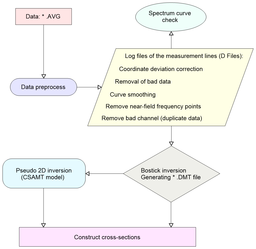
The main components of the CSAMT-SW framework are: (1) Transformation from AVG to D format; (2) Editing CHK data and converting to D format; (3) Manual data checks: gap filling, near-field removal; (4) Smoothing based on D-format data; (5) Estimation of correction factors (D, H, K, Z); (6) The Bostick inversions; (7) The Quasi-2D inversions using the global field model (ID), integrating near and transition fields. Post-Bostick inversion results were stored as *_BOS.DAT and *_BSS.DAT, with final inversion-ready data in *_M.DMT. The 2D inversion proceeded until either the RMS error threshold or a five-iteration limit was reached. Final resistivity models (Fig. 3) were cross-validated with local geology and clearly delineated subsurface features, offering a robust interpretation framework.

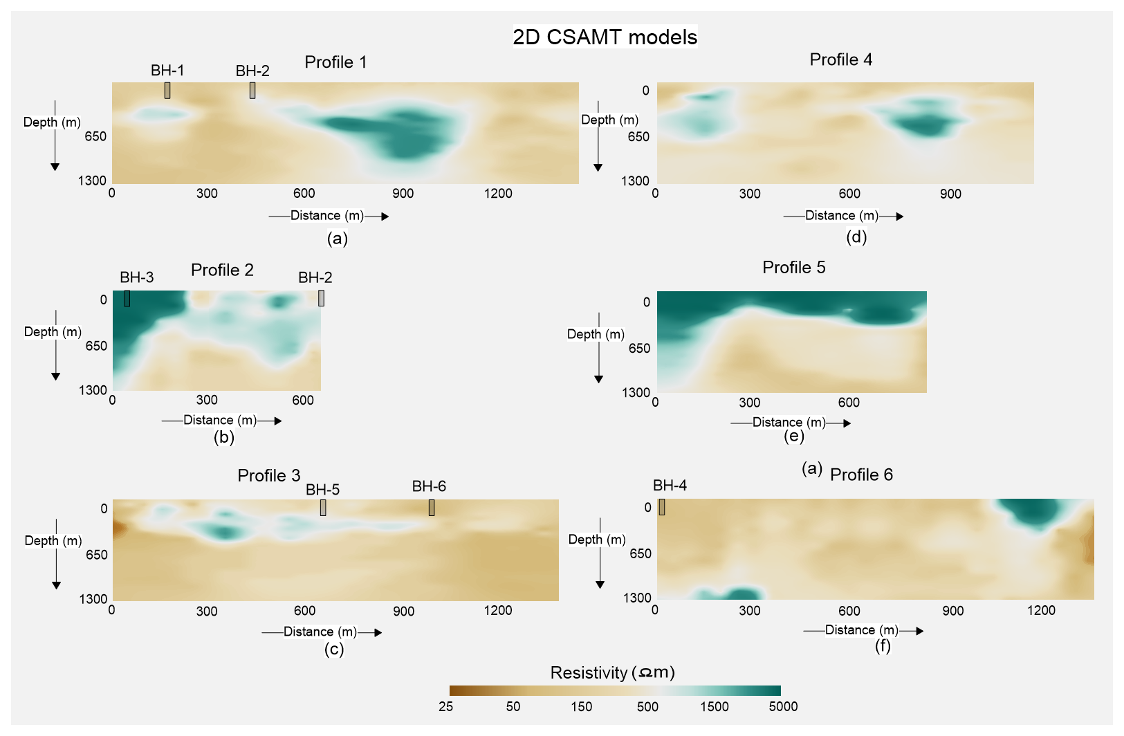
Figure 3 Construction of 2D CSAMT models along six geophysical surveyed lines: (a) Line 1, (b) Line 2, (c) Line 3, (d) Line 4, (e) Line 5, and (f) Line 6. Resistivity values increase from brown to green on the color scale.

2.3 Permeability estimation framework

2.3.1 Laboratory-based permeability determination from borehole core samples

Permeability is a key hydrogeological parameter that quantifies the ability of porous media, such as rock or sediment, to transmit fluids. It governs subsurface fluid flow and plays a central role in groundwater studies (Allègre et al., 2016; Fiandaca et al., 2018; Mudunuru et al., 2022; Esmaeilpour et al., 2023; Carbillet et al., 2024). Permeability reflects how easily fluids move through pore networks or fractures and is typically measured via pumping tests or core analysis, methods that are costly and logistically intensive. It is influenced by porosity, lithology, saturation, structural features (e.g., faults, joints), and diagenetic processes (Dewandel et al., 2006; Yan et al., 2024).

In this study, initial k data from the Jinji region were limited to six boreholes. To strengthen the dataset, 116 lab tests were conducted on core samples from three main lithologies, sandstone (31), hornstone (23), and granite (62), recovered from depths up to 200 m. These data help delineate vertical k trends and refine the region's hydrogeological model. Core recovery employed a wireline rotary system with triple-tube barrels to preserve sample integrity (ISRM, 2015). Samples were vacuum-sealed and stored under controlled humidity to retain in-situ moisture and fracture structure. Prior to testing, cores were trimmed to standard 50 mm × 100 mm cylinders and screened for visible defects. Two laboratory methods were used based on k range. The steady-state flow test with ASTM D5084-24 guidelines (ASTM International, 2024) was applied to higher-k sandstone. A constant hydraulic gradient was applied under fully saturated conditions, and the corresponding volumetric flow rate was recorded. Permeability was determined through the application of Darcy's Law:

$$\begin{array}{}\text{(1)}& k={\displaystyle \frac{Q\cdot \mathit{\mu }\cdot L}{A\cdot \mathrm{\Delta }P}}\end{array}$$

where ΔP is the pressure differential applied across the sample (Pa), A is the cross-sectional area (m²), L is the length of the sample (m), μ is the dynamic viscosity of the fluid (Pa s), and Q is the volumetric flow rate (m³ s⁻¹).

For low-k hornstone and granite, the pulse decay method (Brace et al., 1968) was used. A brief pressure pulse was applied, and pressure decay was monitored under confining stresses up to 30 MPa to simulate in-situ conditions and assess stress-dependent k behavior. Tests were conducted under both dry and saturated conditions to evaluate moisture sensitivity. Replicate measurements ensured data reliability, and statistical analyses assessed intra- and inter-lithology variability. Results revealed that granite had the lowest k due to its dense crystalline structure, while hornstone showed intermediate values, likely due to localized fracturing. Sandstone exhibited the highest k, particularly at greater depths, confirming its role as the primary aquifer unit in the region.

2.3.2 Permeability-resistivity relationship: Archie's law and the role of Kozeny–Carman

Numerous foundational studies have linked electrical resistivity to hydraulic properties like k. A prominent example is the Archie equation (Archie, 1942), which relates resistivity to porosity and water saturation in clean, saturated sediments. However, its assumption of clay-free conditions limits its applicability in complex or clay-rich lithologies (Waxman and Smits, 1968; Glover, 2015). It is commonly expressed as:

$$\begin{array}{}\text{(2)}& {\mathit{\rho }}_{\mathrm{b}}=a\cdot {\mathit{\rho }}_{\mathrm{f}}\cdot {\mathit{\varphi }}^{-m}\end{array}$$

In this equation, ϕ is porosity, ρ_f is fluid resistivity, ρ_b is bulk resistivity, and a and m are empirical constants. Although Archie's law does not directly yield k, porosity serves as a useful proxy due to its strong influence on fluid movement. As such, the resistivity–porosity relationship can be leveraged to infer k indirectly, especially when supplemented with additional petrophysical frameworks (Revil and Cathles, 1999).

The Kozeny–Carman equation, though not used explicitly in this study, provides a widely accepted theoretical foundation that connects k to porosity and specific surface area (DallaValle, 1956; Bear, 1972). While it does not incorporate resistivity directly, this model is often used in hydrogeophysical studies to support the interpretation of petrophysical relationships that bridge electrical and hydraulic properties (Chapuis and Aubertin, 2003). Its relevance lies in the broader theoretical justification for using porosity, derived or inferred from resistivity, as a predictor of k. The application of this equation alongside Archie's law facilitates the development of empirical or semi-empirical models that connect electrical resistivity to k (Glover, 2009; Yan et al., 2024).

However, direct application of these equations to complex geological environments, such as fractured granite, sandstone, and hornstone, remains limited due to heterogeneities in mineral composition, pore connectivity, and structural anisotropy. To mitigate such constraints, our approach empirically develops a localized, site-calibrated correlation involving k and resistivity, grounded in co-located deep borehole and CSAMT data. This empirical link supports high-resolution spatial modeling of k in both 2D and 3D for the Jinji area, offering enhanced insight into subsurface hydrogeological conditions where traditional models may not be applicable.

2.3.3 Spatial permeability modeling from CSAMT data

To estimate permeability across the entire study area, we employed a multi-stage approach integrating borehole core analysis with CSAMT-derived resistivity data. In the first stage, a total of 116 laboratory-based k measurements were acquired using 6 drilling tests (from BH-1 to BH-6) with 0–200 m depth (Fig. 4). The k measurements were obtained from intact rock core samples representing three principal lithologies: granite, hornstone, and sandstone.

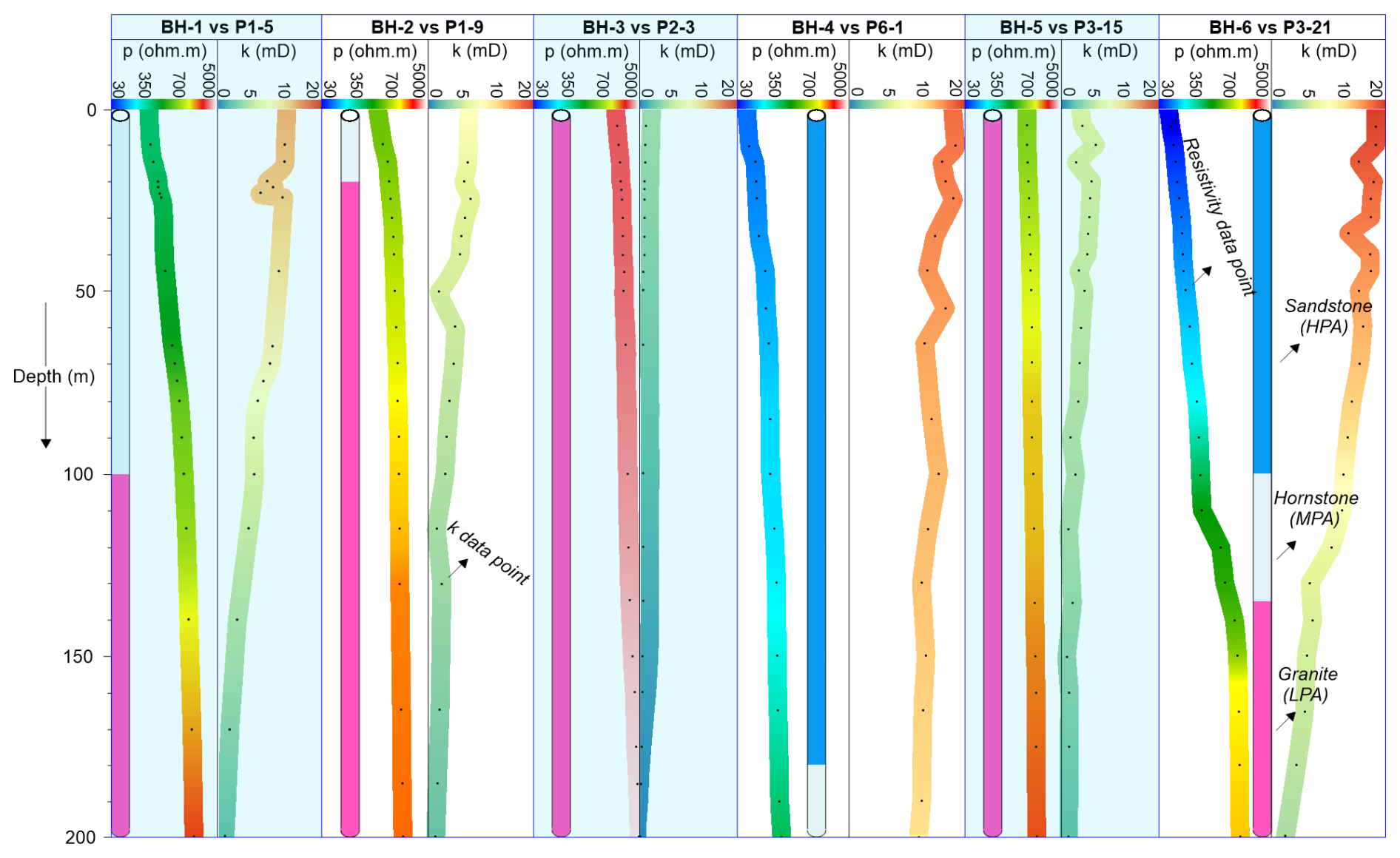
Figure 4 Comparison of 116 CSAMT-based resistivity (ρ) data points with corresponding drilling-based permeability (k) values at depths of 0–200 m across six borehole locations (BH-1 to BH-6). The data were used to evaluate high potential aquifers (HPA) in sandstone, medium potential aquifers (MPA) in hornstone, and low potential aquifers (LPA) in granite. Each dot represents a resistivity or permeability data point. Sounding labels indicate specific CSAMT locations: P1-5 (5th point on line 1), P1-9 (9th on line 1), P2-3 (3rd on line 2), P6-1 (1st on line 6), and P3-15 and P3-21 (15th and 21st on line 3).

In the second stage, each of the 116 borehole-derived k values was empirically correlated with corresponding resistivity values extracted from CSAMT soundings co-located with the borehole sites. The spatial correspondence between boreholes and CSAMT sounding points was carefully matched (Fig. 4). For example: P1-5 represents the fifth CSAMT sounding at 200 m along survey line 1 near borehole BH-1; P1-9 corresponds to the ninth sounding at 400 m on line 1 near borehole BH-2; P2-3 denotes the third sounding at 100 m along line 2 near BH-3; P6-1 indicates the first sounding at 0 m on line 6 adjacent to BH-4; P3-15 and P3-21 represent the fifteenth (700 m) and twenty-first (1000 m) soundings along line 3, near boreholes BH-5 and BH-6, respectively.

In the third stage, all 116 paired measurements of k and ρ were utilized to develop an empirical model. An exponential relationship was derived between permeability (k in millidarcies or mD) and electrical resistivity (ρ in Ωm), expressed as follows (Fig. 5):

$$\begin{array}{}\text{(3)}& k=\mathrm{15.373}{e}^{-\mathrm{0.002}\mathit{\rho }}\end{array}$$

This site-specific empirical model was then applied to the entire suite of CSAMT resistivity data collected along six survey profiles to estimate spatial variations in k across the broader study area. Using this relationship, we generated predictive 2D and 3D k models that capture the hydraulic behavior of three major lithological units: low potential aquifer (LPA): associated with low-permeability granite, medium potential aquifer (MPA): hosted within fractured hornstone (hornfels), high potential aquifer (HPA): corresponding to more porous sandstone units.

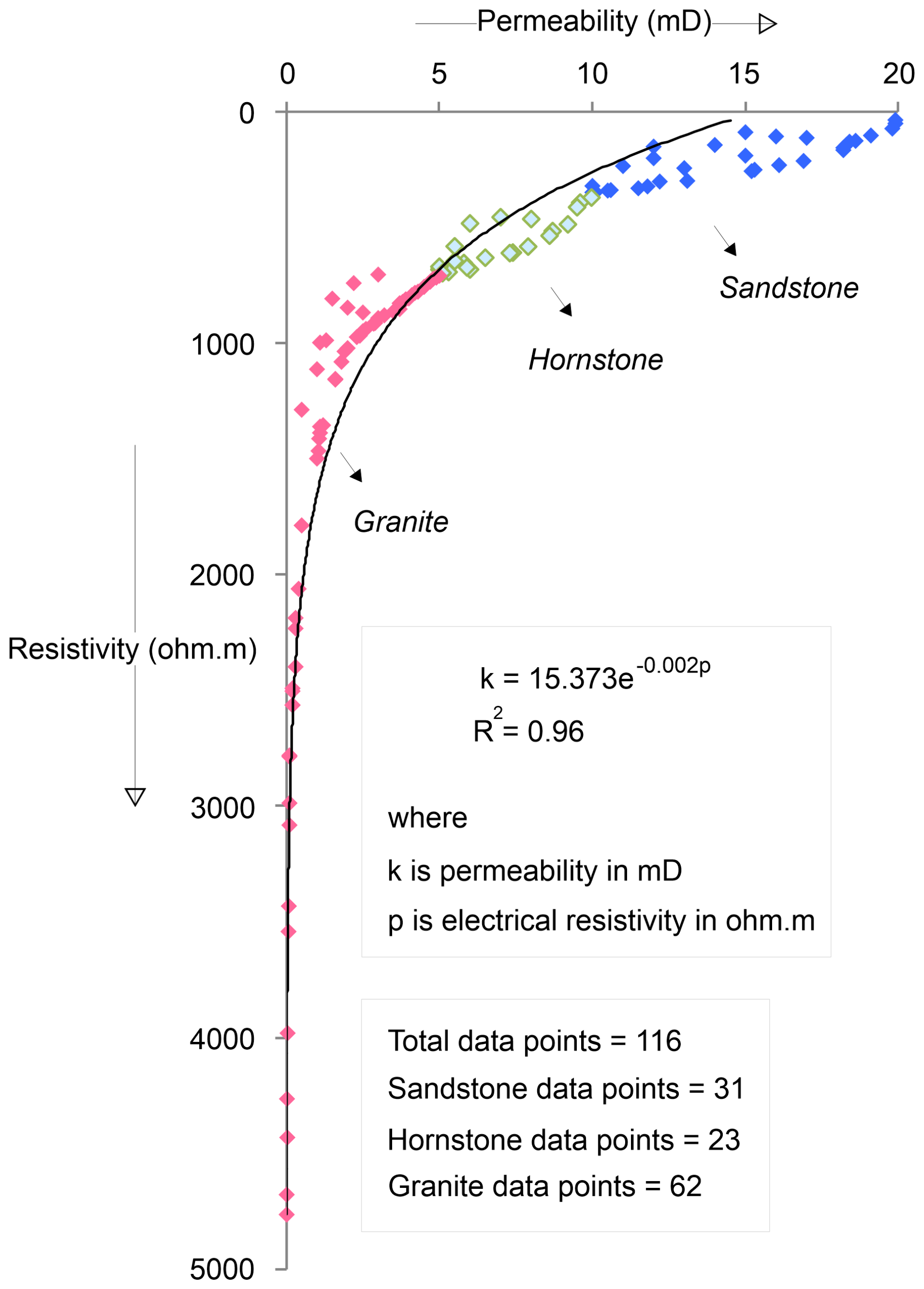
Figure 5 Empirical relationship derived from 116 data points comparing CSAMT-based resistivity and drilling-based k at depths of 0–200 m, across three lithologies: sandstone (31 data points), hornstone (23 data points), and granite (62 data points).

These models provide a depth-resolved assessment of subsurface k reaching depths of up to 1300 m below the surface. Final 2D and 3D spatial visualizations were developed by SKUA-GOCAD and Geosoft Oasis montaj modeling software (Webring, 1981; Mira Geoscience Ltd., 1999; Hasan et al., 2025), enabling the visualization of k distributions across all six CSAMT profiles and improving hydrogeological characterization in structurally complex hard rock terrain.

3 Results

3.1 Cross-validation of geophysical and borehole parameters

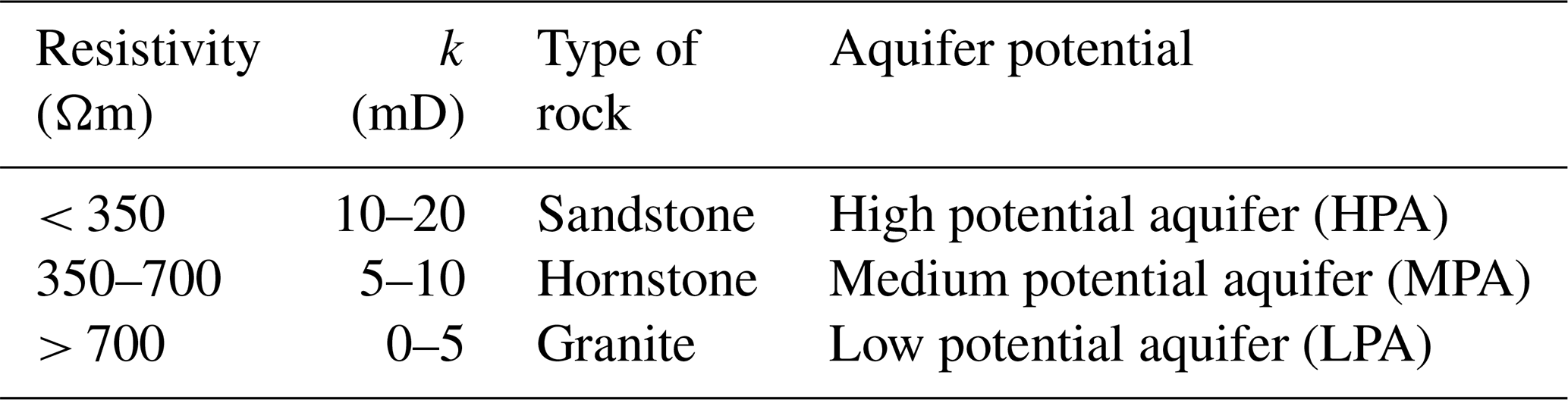
Table 2 summarizes the integrated dataset from 6 drills and 6 geophysical profiles to resolve the spatial structure of the subsurface into three distinctive hydrogeological units, based on variations in electrical resistivity and corresponding k values. The development of these subsurface models mainly depends on borehole data, CSAMT-derived resistivity measurements, and the regional geological framework. The stratigraphy was categorized into three primary lithologies: sandstone, hornstone, and granite. Classification criteria were established as follows: sandstone was defined by resistivity values below 350 Ωm and a k range of 10–20 mD; hornstone exhibited resistivity values between 350 and 700 Ωm with a k range of 5–10 mD; and granite was characterized by resistivity values exceeding 700 Ωm and k values ranging from 0 to 5 mD. Based on our evaluations of the subsurface hydrogeological model's aquifer potential zones, we found that sandstone contains the high potential aquifer (HPA), hornstone contains medium potential aquifer (MPA), and granite has low potential aquifer (LPA). Aquifers with the largest yields or the best water-bearing capacity are indicated by sandstone, whereas aquifers with the lowest yields or the worst water-bearing capacities are denoted by granite. Groundwater development is best facilitated by sandstone in the study area, whereas groundwater extraction is most hindered by granite.

Table 2 Integrating distinct ranges of electrical resistivity and k enables a comprehensive assessment of groundwater potential across various hard rock types.

3.2 2D groundwater assessments

Using geophysical-borehole correlation as its basis, Eq. (3) efficiently converts 2D CSAMT models (Fig. 3) into 2D k models (Fig. 6). The interpreted 2D k models shown in Fig. 7, in comparison with the limited borehole experiments, allow for a comprehensive assessment of the groundwater resources in hard rock across the whole research area, from 0 to 1300 m deep.

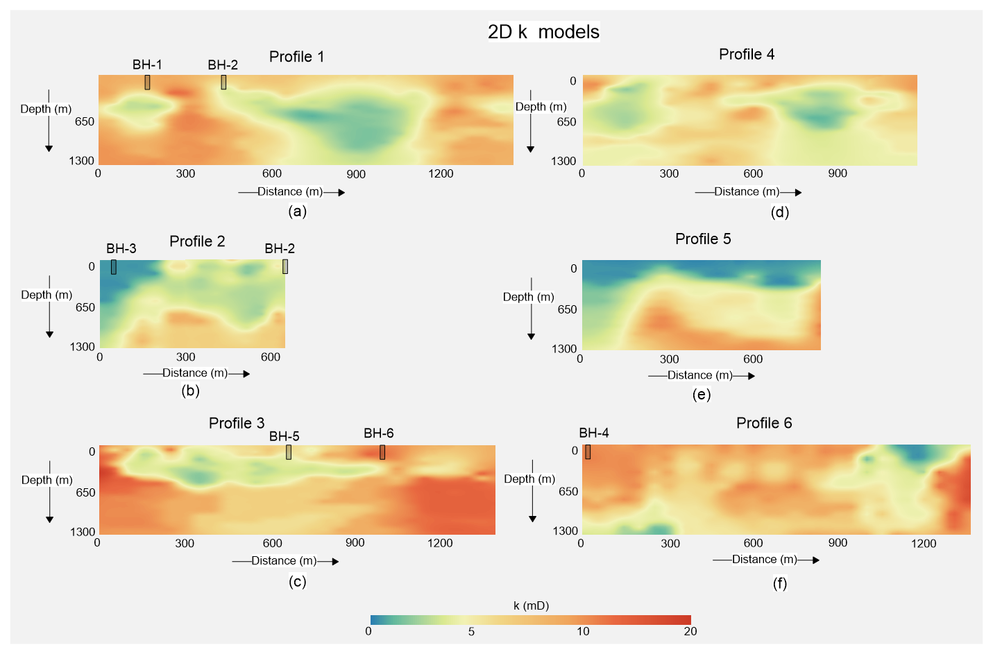
Figure 6 The predicted 2D k models along six geophysical surveyed lines: (a) Line 1, (b) Line 2, (c) Line 3, (d) Line 4, (e) Line 5, and (f) Line 6. k values increase from blue to red on the color scale.

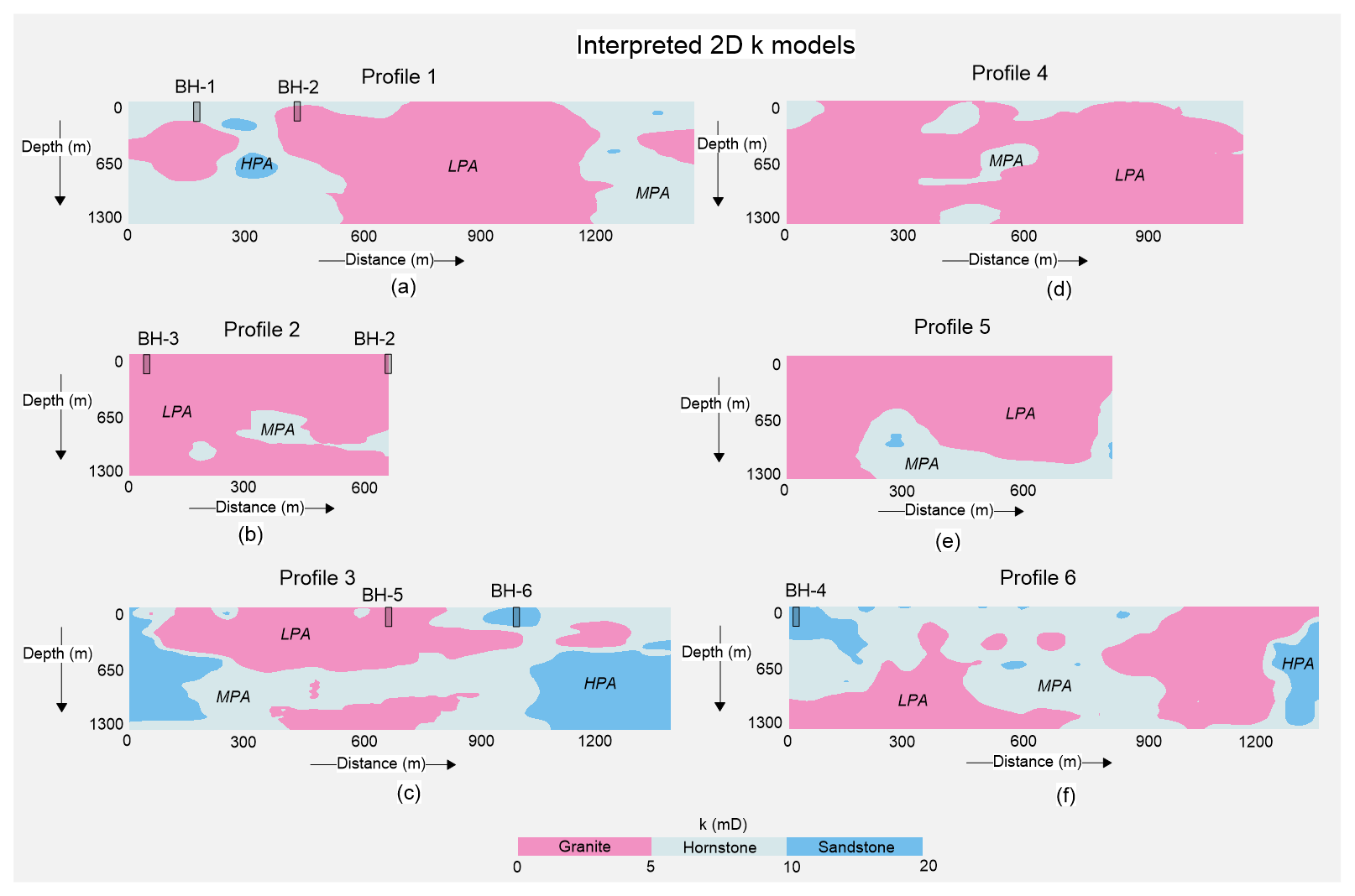
Figure 7 The interpretation of the predicted 2D k models along six geophysical surveyed lines: (a) Line 1, (b) Line 2, (c) Line 3, (d) Line 4, (e) Line 5, and (f) Line 6. Sandstone is represented in blue, hornstone in light blue, and granite in pink.

The integrated 2D k models (Fig. 8) and their interpretations (Fig. 9) provide a detailed evaluation of groundwater potential across complex geological settings of sandstone, hornstone, and granite. Profile 1 reveals a high-potential sandstone aquifer (85–305 m thick) between 245–380 m distances at 205–400 m depth. Medium-potential hornstone aquifers are found from 0–525 and 1185–1445 m distance down to 1300 m. Low-potential granite aquifers appear at 0–285 m (290–790 m depth), 385–1185 m (full depth), and 1305–1450 m (390–745 m depth). Profile 2 shows a medium-potential hornstone aquifer with 140–380 m thickness (490–1105 m depth) between 145–215 and 290–645 m distance. No high-potential sandstone aquifers are present. Granite dominates (0–700 m distance, 0–1300 m depth) the profile with low yield except in hornstone zones. Profile 3 contains both high-potential sandstone (0–250, 905–1065, and 1040–1390 m distances at respective depths of 0–1190, 0–205, and 490–1305 m) and medium-potential hornstone aquifers (full depth with 0–1400 m distance) across the entire surveyed line. Granite aquifers are assessed at 80–1015 m (0–590 m depth), 395–845 m (915–1300 m depth), and 1100–1300 m (200–500 m depth). Profile 4 features medium-potential hornstone at 0–105 m (0–340 m depth), 340–645 m (0 to 1300 m depth), 595–790 m (0–300 m depth), and 1015–1145 m (0–345 m depth). No high-potential sandstone is observed. Granite aquifers of low potential dominate (0–1145 m distance between 0–1300 m depth), except in hornstone zones. Profile 5 shows medium-potential hornstone (190–845 m distance, 390–1300 m depth) and two small high-yield sandstone patches (290 m at 790–960 m depth and 815 m at 1045–1135 m depth). Low-potential granite appears at distance 0–190 m (0–1300 m depth) and 790–815 m (0–1025 m depth). Profile 6 includes high-potential sandstone zones at 0–190 m (0–490 m depth) and 1245–1345 m (215–1225 m depth). Low-potential granite is present at 0–690 m (390–1300 m depth) and 790–1360 m (0–1190 m depth), while hornstone with medium potential dominates the remainder. Overall, the southeastern and northwestern zones host abundant medium- to high-potential aquifers, while central regions show limited or poor groundwater prospects.

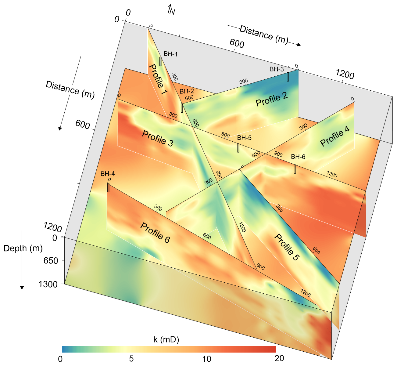
Figure 8 The integrated 2D k models derived from the incorporation of geophysical and drilling data, with k represented on a color bar spanning from green to red.

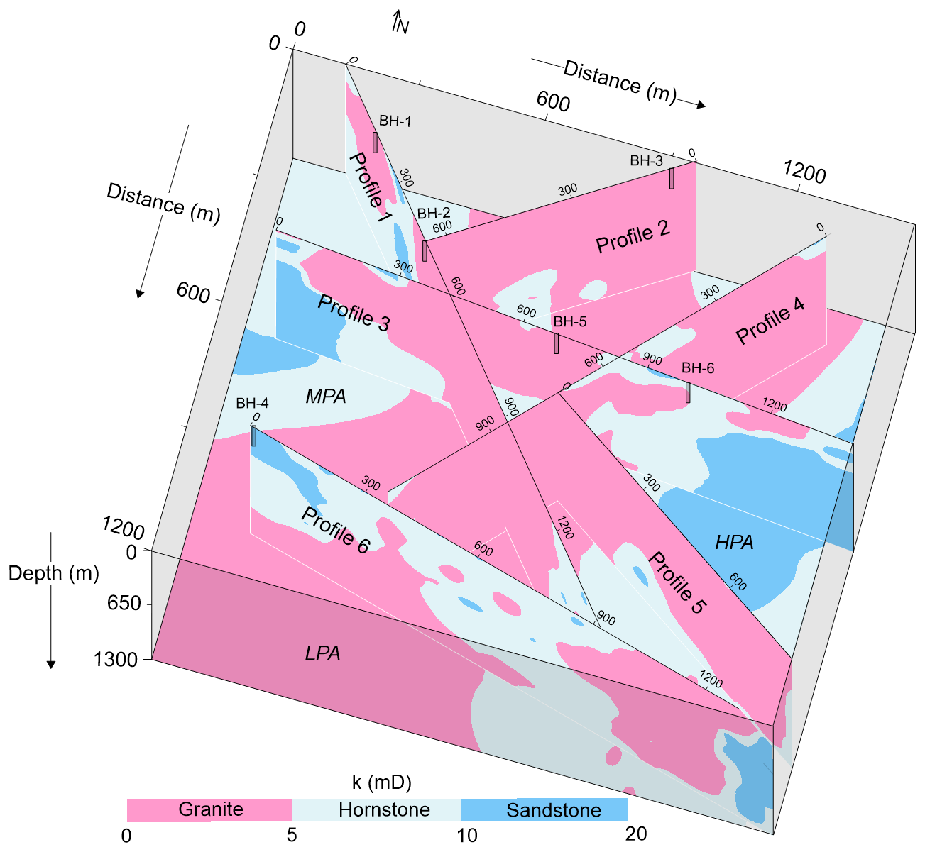
Figure 9 Analysis of 2Dk models, based on defined k ranges, for three groundwater potential aquifers: low potential aquifer (LPA), medium potential aquifer (MPA), and high potential aquifer (HPA), corresponding to the granite, hornstone, and sandstone formations, respectively.

3.3 3D groundwater assessments

The 3D k (outer view) visualization (Fig. 10a, b) provides a comprehensive assessment of the water-bearing capacity of the rock mass. Low-potential granite aquifers are found at the surface along: line 1 (85–215, 385–1175 m), line 2 (0–655 m), line 3 (0–45, 95–175, 265–585, 605–845, 1145–1315 m), line 4 (90–390, 490–615, 745–1115 m), line 5 (0–815 m), and line 6 (1045–1345 m). Medium-potential hornstone aquifers appear along: line 1 (0–95, 190–260, 295–415, 1185–1425 m), line 3 (40–105, 215–275, 580–605, 850–910, 1010–1155, 1310–1410 m), line 4 (45–90, 390–490, 590–685, 1115–1185 m), and line 6 (90–190, 215–275, 315–485, 505–605, 635–1045 m). High-potential sandstone aquifers are identified in: line 1 (265–310 m), line 3 (235–255, 915–1010 m), line 4 (0–45 m), and line 6 (0–90, 210–225, 275–305, 515–525, 605–635 m), Overall, Fig. 10a, b shows that higher-yield aquifers are mainly concentrated in the southern portion of the investigated site.

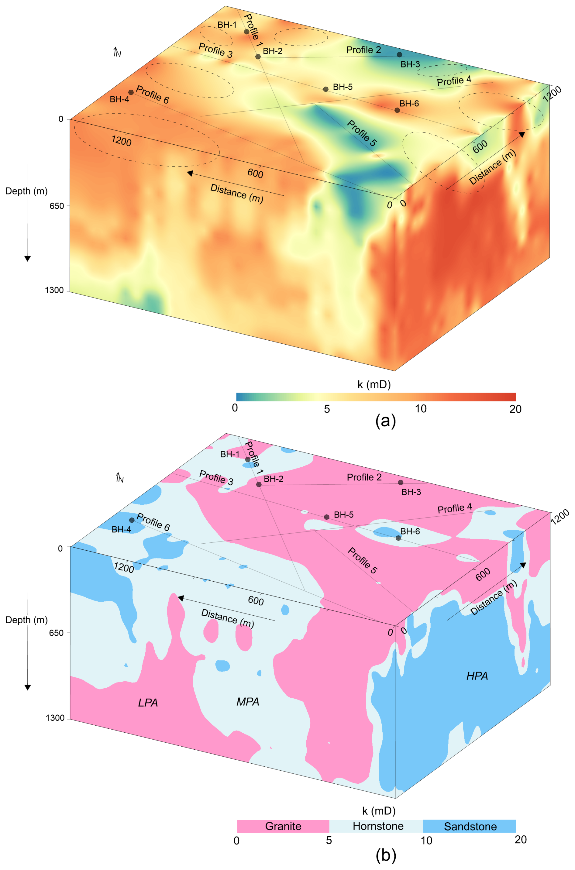
Figure 10 The 3D k models (CSAMT-based), with k shown on a color scale increasing from green to red, correspond to three groundwater potential aquifers: low potential aquifer (LPA), medium potential aquifer (MPA), and high potential aquifer (HPA), associated with three geological strata: granite, hornstone, and sandstone, respectively. The uncertainty contours (highlighted by areas with black dots) indicate zones of reduced confidence in k estimation. (a) The exterior visualization of the 3D k model, and (b) the analysis of the 3D k model from an external perspective.

Figure 11a, b shows a 3D internal view of aquifer potential at 1300 m depth. Low-yield granite aquifers are identified along: surveyed line 1 (515–1215 m), line 2 (0–290 m), line 3 (390–690 m), line 4 (0–1145 m), line 5 (0–195, 565–595 m), and line 6 (0–690, 1075–1115 m). Medium-potential hornstone aquifers are found along: profile 1 (0–540, 1215–1445 m), profile 2 (295–675 m), profile 3 (175–395, 445–815, 915–1035 m), profile 5 (205–565, 610–815 m), profile 6 (685–1080, 1110–1355 m). High-potential sandstone aquifers appear along: profile 3 (0–205, 1010–1400 m) and profile 5 (810–815 m). Overall, medium to high potential aquifers are mainly distributed in the southeastern and northwestern regions, while central areas are dominated by low-yield granite. The aerial 3D k model enhances visualization of aquifer distribution, supporting accurate groundwater assessment.

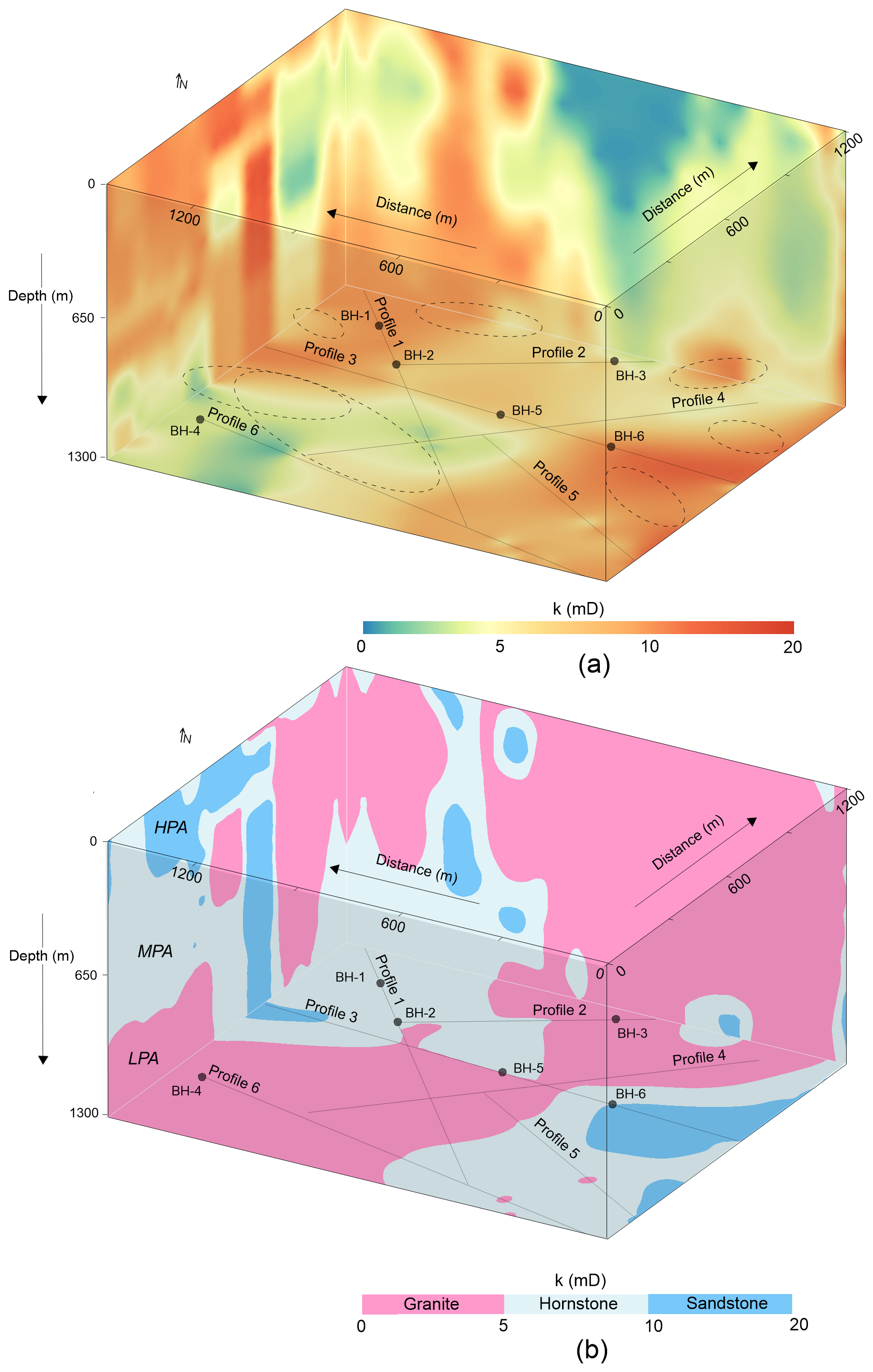
Figure 11 The 3D k models (CSAMT-based), withk represented on a color scale ranging from green to red, illustrate three groundwater potential aquifers: low potential aquifer (LPA), medium potential aquifer (MPA), and high potential aquifer (HPA), associated with three geological strata: granite, hornstone, and sandstone, respectively. The uncertainty contours (highlighted by areas with black dots) indicate zones of reduced confidence in k estimation. (a) The interior visualization of the 3D k model, and (b) the analysis of the 3D (internal perspective) k model.

3.4 Depth-wise groundwater assessments

Due to limited borehole data, direct estimation of k below 200 m is not feasible. However, by integrating borehole and CSAMT data, k values could be reliably estimated down to 1300 m. This approach enabled efficient and detailed evaluation of hard rock aquifers using both 2D and 3D models (Fig. 12), with k values extracted at depths of 0, 200, 600, 1000, and 1300 m. At 1300 m, over 42 % of the subsurface in the southwest and northeast comprised low-yield granite. Hornstone accounted for 40 % (medium yield) near granite zones in the northwest and southeast, while high-yield sandstone made up 18 % in the east. At 1000 m, sandstone (15 %) was concentrated in the southeast (high yield), hornstone (38 %) in the southeast and northwest (medium yield), and granite (47 %) dominated the central and boundary zones (low yield). At 600 m, the subsurface was 55 % granite (central and northern zones, low yield), 32 % hornstone (western region, medium yield), and 13 % sandstone (southeast, high yield). At 200 m, granite dominated 64 % of the center and north (low yield), hornstone made up 26 % in the south (medium yield), and sandstone (10 %) in the west was associated with high yield. At 0 m, 73 % of the central area comprised low-yield granite, 20 % of the southwest was hornstone (medium yield), and 7 % sandstone (high yield) was concentrated in the southwest.

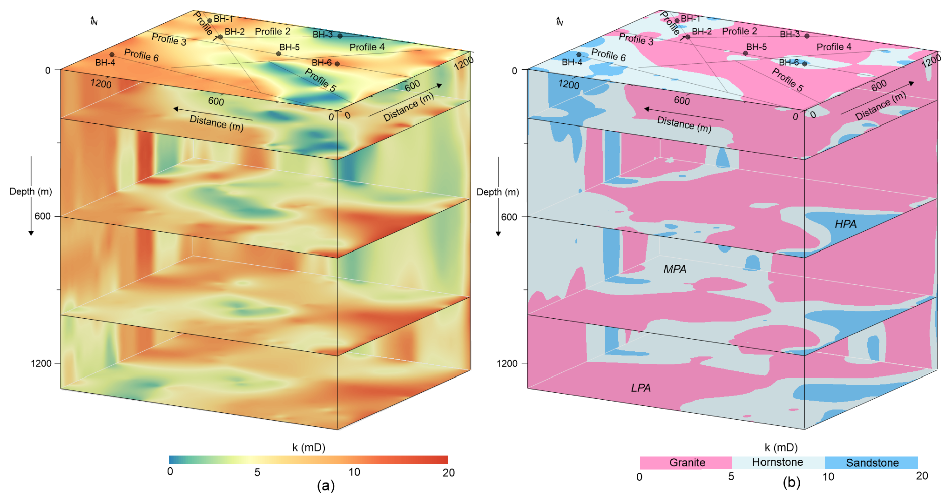
Figure 12 (a) Geophysical k imaging at depths of 0, 200, 600, 1000, and 1300 m, with k shown on a color scale increasing from green to red. (b) Evaluation of CSAMT-derived k values (based on defined k ranges) at various depths for different aquifer types: low potential aquifer (LPA) in granite, medium potential aquifer (MPA) in hornstone, and high potential aquifer (HPA) in sandstone.

Overall, Fig. 12 shows a decrease in low-yield granite thickness with depth. Groundwater potential is lowest around 600–700 m depth, while deeper zones (> 700 m) in the northwest, southeast, and southwest show more favorable aquifer conditions.

3.5 Validation of predicted vs. measured permeability

Groundwater evaluation was greatly improved by systematic CSAMT-based k estimation using Eq. (3). As shown in Figs. 6–12, granite dominates the central, northeastern, and southwestern zones; hornstone occurs mainly in the southeast, west, and northwest; and sandstone is prevalent in the east. Borehole-based assessments are limited by inconsistent subsurface mapping. While k values align near 200 m depth, broader extrapolation remains uncertain, highlighting the limitations of sparse drilling in complex geology.

Table 3 Percentage match and deviation between the measured k and the predicted k^′ for 18 selected data points out of the total 116.

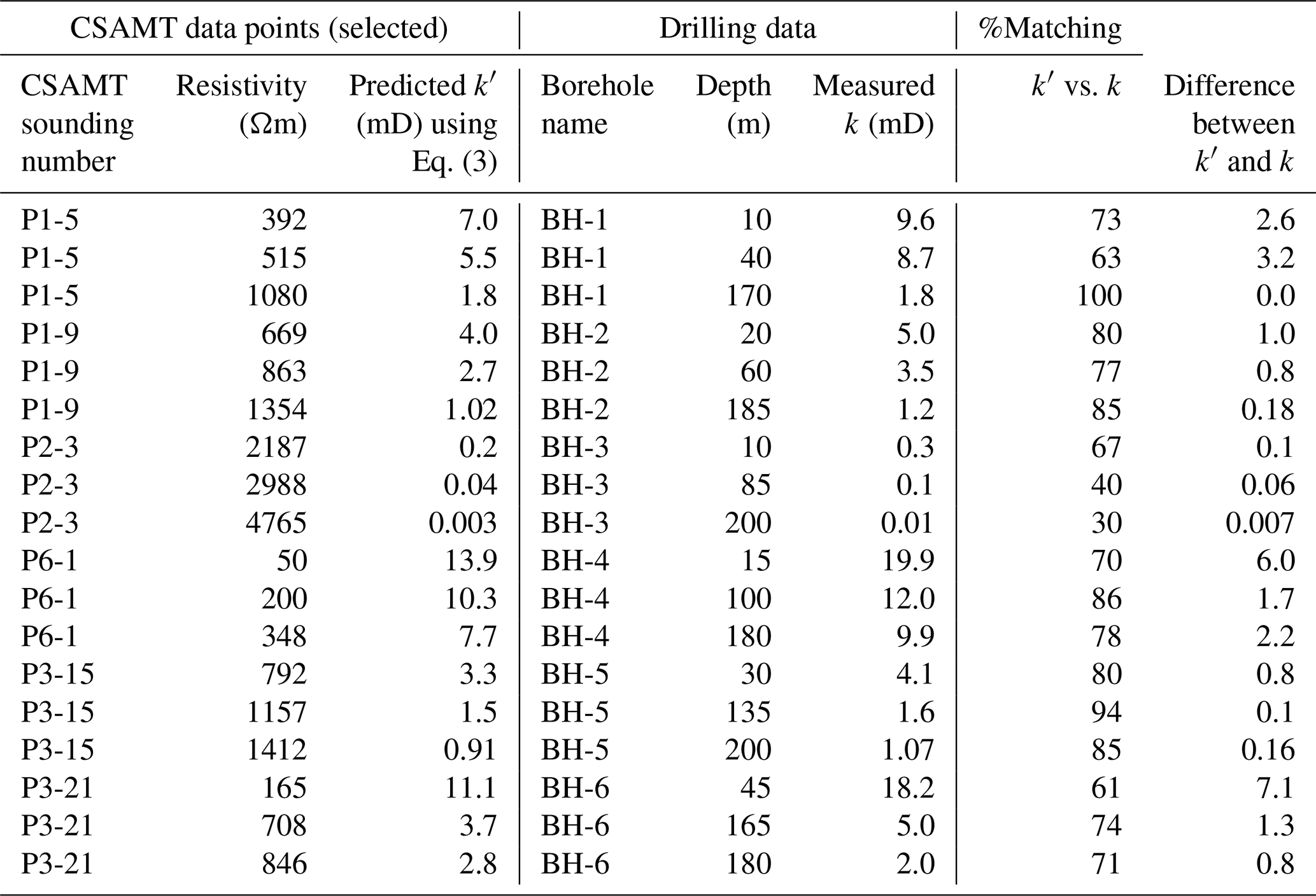
To clarify the basis of the percentage matching values, the following explicit equation was used to quantify the agreement between CSAMT-derived k^′ values and borehole-based k estimates:

$$\begin{array}{}\text{(4)}& \mathrm{Percentage}\mathrm{Match}=\left({\displaystyle \frac{min(k,k^{\prime })}{max(k,k^{\prime })}}\right)\times \mathrm{100}\end{array}$$

Here, min ($k,k^{\prime }$) is the smaller of the two permeability values, either the measured permeability (k) from borehole data or the estimated permeability (k^′) from the CSAMT model, at a given depth. Conversely, max ($k,k^{\prime }$) is the larger of the two values. This ratio offers a normalized agreement metric, where 100 % indicates a perfect match and lower values reflect greater divergence. Table 3 summarizes results for 18 representative data points (out of 116 total calibration points). Percentage matches range from 30 % to 100 %. Higher agreement is generally observed in moderate-resistivity formations, whereas lower matches occur primarily in highly resistive, low-permeability granite units (e.g., BH-3), where small absolute differences produce larger relative deviations. Despite local discrepancies, both predicted and measured values consistently classify the same aquifer potential zones.

Because the empirical model was derived from 116 paired measurements, predictive capability was evaluated using leave-one-point-out cross-validation (LOOCV). Each observation was excluded sequentially; the regression was recalibrated using the remaining 115 data points; and permeability was predicted for the excluded point. Prediction error was quantified using the root mean square error (RMSE):

$$\begin{array}{}\text{(5)}& \mathrm{RMSE}=\sqrt{{\displaystyle \frac{\mathrm{1}}{n}}{\sum }_{i=\mathrm{1}}^n{\left(k_i-k_i^{\prime }\right)}^{\mathrm{2}}}\end{array}$$

where k_i denotes the measured permeability, $k_i^{\prime }$ represents the predicted value for the excluded observation, and n = 116 is the total number of paired resistivity–permeability data points used in the cross-validation procedure. This procedure yielded:

$$\begin{array}{}\text{(6)}& {\mathrm{RMSE}}_{\mathrm{LOOCV}}=\mathrm{2.36}\mathrm{mD}\end{array}$$

Given the observed permeability range (0.01–19.9 mD), this error indicates stable predictive performance within the calibration domain. For the representative points listed in Table 3, LOOCV-predicted permeability values differ only slightly from those obtained using the full regression model, indicating that the fitted relationship is not strongly influenced by individual observations.

To further assess spatial transferability, a leave-one-well-out cross validation was conducted. In this approach, all data from one borehole were excluded, the regression was recalibrated using the remaining wells, and permeability was predicted for the omitted well. Using the same RMSE formulation (Eq. 5), this yielded:

$$\begin{array}{}\text{(7)}& {\mathrm{RMSE}}_{\mathrm{well}}=\mathrm{2.78}\mathrm{mD}\end{array}$$

The modest increase in error relative to pointwise LOOCV reflects geological heterogeneity rather than model instability. This result demonstrates that the empirical resistivity–permeability relationship generalizes reasonably well across different boreholes and lithological domains.

Together, percentage agreement, leave-one-point-out validation, and leave-one-well-out validation demonstrate that the CSAMT-derived empirical model provides robust and transferable permeability estimates within the measured range. Although localized deviations occur, likely due to structural anisotropy and fracture-controlled flow, the regression is not dominated by single data points or individual wells, supporting its application for regional-scale groundwater assessment.

4 Discussion

4.1 Scalable geophysical approach for deep groundwater modeling

The integration of geophysics into groundwater studies provides an efficient and scalable substitute for borehole-based methods, especially in deep and geologically complex terrains. While boreholes provide direct k data, their use is limited by cost, logistics, and sparse coverage. Our study presents a robust framework for 2D and 3D k modeling beyond 1 km depth by integrating CSAMT with borehole data in a lithologically diverse setting. This approach addresses key challenges in areas with limited surface water and low-k granite near the surface, revealing deeper fractured zones with higher groundwater potential in granite, hornstone, and sandstone. These deep aquifer insights support China's national water security strategies and inform sustainable groundwater management under climate stress.

4.2 Ensuring data quality and model reliability

To minimize uncertainty and enhance accuracy, we implemented a rigorous workflow throughout data acquisition, processing, inversion, and modeling. For CSAMT, this included careful survey planning, optimized electrode configurations, and the application of advanced filtering and static shift corrections. Inversion was guided by multidimensional modeling constrained by borehole-derived a priori information, improving resolution and mitigating non-uniqueness. Permeability measurements were obtained under controlled laboratory conditions using high-quality, undisturbed core samples from six boreholes, reducing discrepancies between laboratory and field scales. These measures, together with integrated lithological data, enabled the development of a robust k model suitable for reliable groundwater assessment across the study area.

4.3 Comparative advantages of CSAMT for deep hard rock aquifer characterization

CSAMT, developed in the 1970s, remains uniquely valuable for deep subsurface exploration, particularly in resistive and fractured hard rock environments. Its ability to image at intermediate-to-deep depths (hundreds to over a thousand meters) with relatively high resolution and controlled signal strength enhances its ability to delineate lithological contacts and fluid-bearing formations where other resistivity methods (VES and ERT) may fall short. While electromagnetic methods such as MT and TDEM are also capable of probing deep subsurface structures, achieving comparable results in similarly complex hard rock settings presents notable challenges. MT, which relies on natural variations in electromagnetic fields, can reach even greater depths than CSAMT and has been successfully applied in regional-scale hydrogeological investigations, such as identifying deep groundwater circulation paths in mountain systems (Jiang et al., 2014) and tracing flow systems that recharge lowland aquifers (Gonzalez-Duque et al., 2024).

As summarized in Table 1, MT provides exceptional penetration (tens of kilometers) but has reduced resolution in the upper crust and is highly sensitive to cultural noise, limiting its suitability for detailed k-modeling at the site scale. TDEM, while rapid and effective for intermediate depths, suffers loss of sensitivity in highly resistive formations, making it less effective for fractured granite and hornstone settings. In contrast, CSAMT's controlled-source design and strong immunity to cultural noise provide a balance of penetration depth and resolution well-suited for site-specific groundwater studies in hard rock terrains.

Thus, the comparative analysis (Table 1) underscores why CSAMT is the most appropriate method for this study: it bridges the gap between large-scale regional techniques (MT, TDEM) and shallow, high-resolution methods (VES, ERT), enabling robust 2D and 3D hydrogeophysical modeling essential for evaluating deep aquifer potential.

4.4 Calibrated resistivity thresholds for lithological and hydraulic discrimination

We developed a robust empirical relationship between resistivity and k using 116 co-located data pairs, 62 from granite, 31 from sandstone, and 23 from hornstone, spanning 35–4765 Ωm and 0.01–19.9 mD, respectively. The strong correlation (R² = 0.96) ensures reliable k prediction and minimizes lithological bias. The lithological classification derived from the resistivity–permeability relationship in this study is both geologically plausible and empirically supported by borehole data and field observations. Specifically, granite showed high resistivity (> 700 Ωm) and low k (0–5 mD), hornstone had intermediate resistivity (350–700 Ωm) and moderate k (5–10 mD), and sandstone was marked by low resistivity (< 350 Ωm) and higher k (10–20 mD). These ranges align with the distinct hydrogeological behaviors of each lithology under the site-specific structural and mineralogical conditions. The resistivity thresholds were selected through an integrated approach combining lithological logs from boreholes, established empirical resistivity values reported in the literature, and the geoelectrical contrasts identified in CSAMT profiles. For instance, the high resistivity of granite reflects its dense, low-porosity matrix and limited fluid content, whereas the lower resistivity of sandstone and hornstone corresponds to increased pore connectivity and higher saturation, often associated with structural features or thermal alteration. To ensure robust classification, the resistivity thresholds were calibrated using co-located borehole observations from multiple calibration sites and iteratively refined to maximize agreement between observed lithology and the modeled resistivity–permeability domains. While we acknowledge that resistivity can vary within a given lithology due to localized factors such as fluid saturation, mineral alteration, or fracture density, sensitivity analyses indicated that moderate adjustments to the threshold values had minimal impact on the overall lithological classification or the interpretation of k trends. This suggests that the chosen thresholds are well-suited to the structurally complex Jinji area. Nevertheless, we emphasize that these resistivity–permeability associations are localized and should be recalibrated to account for site-specific conditions before use elsewhere. Although site-specific, the approach demonstrates how minimal calibration data can support high-resolution 2D/3D k modeling in data-scarce settings. Future studies could benefit from probabilistic classification schemes or machine learning approaches to further refine lithological mapping in geologically heterogeneous terrains.

4.5 Impact of lithological and measurement variability on the resistivity–permeability relationship

The fitted relationship between resistivity and k, as illustrated in Fig. 5, is shaped by several factors, including the geological setting, lithological heterogeneity, data distribution, and the accuracy of both measurements. The broad dynamic range in our dataset provides a strong basis for identifying trends across the three dominant lithologies: sandstone, granite, and hornstone. This broad range is especially beneficial for resolving low-k formations such as granite, where k remains uniformly low and shows minimal fluctuation. In these settings, even large shifts in resistivity translate to relatively small changes in k, resulting in a gently declining inverse relationship. In contrast, at lower resistivity values (e.g., < 1000 Ωm) where k exceeds 2 mD, small resistivity shifts result in larger changes in k, leading to a more scattered and nonlinear correlation. This pattern is geologically realistic and reflects the inherent variability of fractured and porous zones in complex lithologies.

4.6 Model validation and predictive reliability

Matching between measured and predicted permeability (k vs. k^′) was also rigorously validated (Table 3). Among 18 selected points from boreholes, 10 showed a difference of less than 1 mD, with only two exceeding 4 mD. Despite minor deviations, all points were accurately classified by lithology. This confirms the empirical model's reliability and its utility for regional-scale k prediction, even in areas lacking direct measurements. The geophysical model effectively compensates for sparse drilling data, offering a scalable and cost-effective tool for hydrogeological evaluation in hard rock terrains.

4.7 Limited and shallow borehole calibration

A key limitation of this study is the restricted depth range of the calibration dataset. The empirical resistivity–permeability relationship (Eq. 3) was derived from 116 core measurements between 0 and 200 m depth. Application of this relationship to depths approaching 1300 m therefore represents extrapolation beyond the calibrated interval.

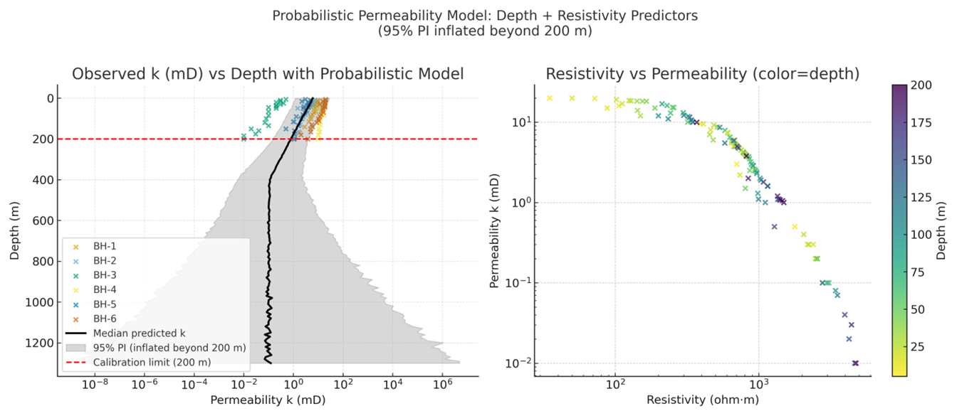
Figure 13 Probabilistic permeability–depth model based on resistivity–permeability calibration from 116 borehole samples (0–200 m). The extrapolation to 1300 m shows increasing uncertainty with depth due to limited calibration data.

To explicitly address this uncertainty, a probabilistic permeability–depth framework was implemented (Fig. 13). Rather than extending Eq. (3) deterministically, prediction uncertainty was propagated from the regression and progressively inflated beyond the 200 m calibration limit. Within the calibrated interval, permeability estimates remain relatively well constrained. Below 200 m, however, the 95 % prediction intervals widen substantially, quantifying decreasing confidence with increasing depth.

Importantly, deep predictions remain conditioned by observed CSAMT resistivity trends and preserve the physically consistent monotonic decrease in permeability with increasing resistivity. Nevertheless, processes not captured by the shallow dataset, such as stress-dependent fracture closure, evolving fracture connectivity, and mechanical anisotropy, may modify permeability behavior at depth. While the probabilistic framework constrains extrapolation risk, it does not eliminate structural uncertainty. Deep borehole testing and stress-dependent hydraulic measurements are therefore required to validate permeability predictions below the calibration range.

4.8 Choice of core-based permeability measurements versus pumping tests

Although pumping tests are widely regarded as the standard method for estimating aquifer permeability (k), they provide only bulk, large-scale averages of hydraulic conductivity over the tested interval. Such measurements are useful for assessing overall transmissivity but lack the spatial resolution required for detailed 2D or 3D geophysical modeling, where localized contrasts in hydraulic properties are critical. The objective of this study was to capture subsurface heterogeneity at scales compatible with CSAMT-derived resistivity. For this purpose, point-specific k measurements were necessary to ensure that calibration data reflected the same resolution and spatial variability represented in the geophysical models. Core samples, analyzed at discrete depths, offered this localized control and provided a closer match to the spatial scale of CSAMT blocks. Therefore, core-derived k values were used in lieu of pumping tests. While this approach inevitably shifts the focus from bulk aquifer transmissivity to matrix- and fracture-scale variability, it ensures that the calibration dataset is scale-compatible with resistivity measurements, thereby improving the reliability of the empirical k–ρ relationship and supporting more accurate heterogeneity mapping in crystalline terrains.

4.9 Scale effects in permeability estimation

In addition to depth-related extrapolation, permeability estimation in this study is influenced by scale transition between centimeter-scale core measurements and tens-of-meter-scale CSAMT inversions. Core plugs (50 mm × 100 mm) primarily capture intrinsic matrix permeability and fractures intersecting the limited sample volume. In fractured crystalline systems, however, hydraulic flow is governed by connected fracture networks whose representative elementary volume (REV) may exceed the dimensions of a core specimen. Individual cores may therefore not reach the REV of the fractured rock mass, leading to systematic underestimation of bulk hydraulic conductivity.

By contrast, CSAMT inversions resolve an effective bulk resistivity over ∼ 50 × 50 m blocks, integrating matrix and fracture contributions across a much larger volume. The empirical k–ρ relationship thus links matrix-scale permeability measurements with block-scale electrical responses. The dispersion observed in Fig. 5 is therefore not merely statistical noise but a reflection of geological heterogeneity and scale-dependent flow processes.

For example, low k values from intact granite cores may correspond to CSAMT blocks intersecting fracture corridors that enhance effective permeability at the field scale. Conversely, cores intersecting localized fractures may yield elevated k relative to the surrounding bulk medium. Variability in cementation, fracture density, and stress-controlled aperture closure further contributes to scatter.

Bridging this scale gap requires intermediate-scale hydraulic constraints. Integration of packer testing, interval hydraulic testing, borehole geophysics, and pumping tests would help reconcile matrix-scale measurements with field-scale connectivity and better constrain the effective REV of the fractured system. Such multi-scale calibration would reduce uncertainty in empirical relationships and improve permeability modeling in structurally complex crystalline terrains.

4.10 Inflection in the resistivity–permeability relationship: a depth analogue

The empirical resistivity–permeability (k–ρ) relationship developed in this study exhibits a sharp decline in k with increasing resistivity and a clear inflection near 1000 Ωm. This mirrors classic depth–permeability (k–z) trends (e.g., Manning and Ingebritsen, 1999; Saar and Manga, 2004; Ingebritsen and Manning, 2010), where k decreases exponentially at shallow depths and follows a power-law pattern deeper down. However, unlike those models that use depth alone, our resistivity-based approach captures additional controls such as lithology, porosity, fluid content, and fracturing, making it a more localized and physically representative proxy, especially in heterogeneous hard rock settings.

Depth was considered but not used as the primary variable due to strong lateral variations in resistivity and k caused by geological complexity. For instance, in the Jinji area, surface granite shows high resistivity and low k, consistent with standard crustal profiles. However, deeper hornstone and sandstone units exhibit lower resistivity and higher k, contrary to typical depth trends, likely due to localized faulting, thermal alteration, and contact metamorphism that enhance fracture connectivity. The resemblance between our k–ρ curve and established k–z models reinforces its physical validity. The observed transition near 1000 Ωm may reflect a shift from conductive, fractured zones to compact, resistive rock masses. While hybrid models incorporating depth may be useful in future work, our resistivity-based method provides a more reliable and site-specific approach for k estimation in structurally complex terrains.

4.11 Salinity effects and uncertainty in deep fluid properties

The influence of factors beyond lithology, particularly groundwater salinity, on CSAMT-derived resistivity warrants careful consideration. Electrical resistivity is sensitive to porosity, fracture density, mineral alteration, fluid saturation, and fluid resistivity (ρ_f). In this study, the empirical k–ρ relationship was calibrated using core samples from 0–200 m across six boreholes under predominantly fresh groundwater conditions. Regional hydrochemical data from the Geological Survey of China (800–1000 m depth) consistently indicate low salinity, supporting the assumption of fresh groundwater within the investigated interval. However, no direct fluid data are available below ∼ 1 km, and the assumption of fresh conditions at greater depths represents an important model constraint.

To evaluate this uncertainty, a sensitivity analysis was performed. If fluid resistivity were reduced by 50 % due to increased salinity, formation resistivity would decrease proportionally, resulting in higher inferred permeability values when substituted into Eq. (3). Because permeability increases exponentially with decreasing resistivity in the fitted model, this effect is nonlinear and resistivity-dependent. Specifically, halving ρ_f increases inferred k by approximately a factor of 2 at 1000 Ωm, 7 at 2000 Ωm, and up to 18 at 3000 Ωm. These results indicate that salinity effects are modest in low-resistivity formations but may significantly influence permeability estimates in highly resistive deep crystalline units.

Accordingly, the permeability model should be interpreted as valid under the assumption of predominantly fresh groundwater conditions and should not be generalized to saline deep aquifers without recalibration. Future investigations should incorporate deep borehole fluid sampling, downhole conductivity logging, and hydrochemical analyses to directly constrain fluid resistivity and reduce salinity-related uncertainty in deep permeability predictions.

4.12 Uncertainty from model extrapolation and edge effects

The 3D permeability (k) model was constructed by interpolating between 2D CSAMT inversion profiles calibrated with borehole-derived k values from six reference locations. Given the limitations in survey geometry and computational cost, full 3D inversion of the resistivity data was not feasible. Instead, we implemented a geostatistical framework using ordinary kriging, which integrated cross-sectional profiles and applied the resistivity–permeability relationship across the model volume. The interpolation was guided by variogram models tuned to reflect the spatial continuity of lithological units and constrained by borehole control points, thereby maintaining geological consistency. While this approach provides a volumetric representation of k that highlights the distribution of permeable zones, its reliability is scale- and data-density dependent. The model is most robust in the central areas where CSAMT lines intersect and are directly supported by borehole data. In contrast, reliability diminishes in regions between widely spaced profiles and toward the model edges and corners, where no direct constraints exist. Sensitivity analyses, based on alternative variogram structures and comparisons with inverse distance weighting, consistently revealed greater variability and uncertainty in these peripheral zones.

To address this, uncertainty contours were added to Figs. 10 and 11, delineating areas of higher and lower confidence. The black dots marking borehole and survey line positions serve as reference anchors, making it clear that interpolation quality decreases with increasing distance from these control points. As such, interpretations in boundary regions should be treated with caution, particularly where model predictions extend beyond the convex hull of available data. We emphasize that the current model provides a reliable first-order framework for k distribution in the study area, but future improvements should prioritize denser CSAMT line coverage and, where feasible, the use of full 3D inversion techniques. Such approaches would better capture lateral continuity, minimize edge effects, and enhance confidence in the extrapolated 3D structure.

4.13 Limitations of storage characterization

A complete aquifer assessment requires evaluation of both permeability and storage parameters, including specific yield, specific storage, and storativity. This study primarily focuses on delineating spatial variations in permeability (k), referred to here as hydraulic flow potential, using CSAMT-derived resistivity calibrated with borehole data. While this approach provides robust insights into transmissivity patterns and fracture-controlled flow pathways, it does not directly quantify aquifer storage capacity.

Permeability and storage represent distinct hydrogeological properties. High k zones do not necessarily imply high storage if fracture porosity is limited, and conversely, formations with significant porosity may exhibit substantial storage despite moderate permeability. Due to the absence of deep pumping tests, drawdown analyses, and detailed porosity logs, storage parameters could not be independently constrained. As such, the present results characterize relative transmissivity and hydraulic connectivity rather than total extractable groundwater volume.

To avoid overgeneralization, the model outputs should therefore be interpreted as indicators of flow potential rather than comprehensive groundwater resource capacity. Future studies should integrate Nuclear Magnetic Resonance (NMR) logging, borehole geophysical porosity tools, interval hydraulic testing, and aquifer-scale pumping tests to better constrain storage properties alongside permeability. Such multi-parameter characterization would enable more rigorous evaluation of sustainable yield and groundwater resource potential in fractured hard rock systems.

4.14 Optimizing borehole placement for CSAMT calibration

Borehole placement in this study was guided by geological mapping, hydrological relevance, and preliminary CSAMT interpretation to ensure representative coverage of the principal lithologies and structural domains. The six boreholes were used both to calibrate the empirical resistivity–permeability relationship and to validate the CSAMT-derived permeability models. Cross-validation results demonstrate that calibration quality depends more on spatial distribution than on borehole number. Leave-one-out cross-validation (LOOCV) of the 116 paired measurements yielded an RMSE of 2.36 mD, indicating that the regression is not overly sensitive to individual data points. Leave-one-well-out cross-validation resulted in an RMSE of 2.78 mD, showing that the empirical relationship maintains reasonable predictive capability when applied to an entirely excluded borehole. The modest increase in error reflects geological heterogeneity rather than model instability.

These findings suggest that a limited but strategically distributed set of boreholes across key lithological and structural zones can provide stable calibration. Slightly higher prediction errors in highly resistive granite highlight the importance of including structurally complex units in calibration. Future work may further optimize efficiency by integrating preliminary CSAMT results into adaptive drilling strategies, targeting areas of higher uncertainty while minimizing drilling costs.

4.15 Rationale for variable CSAMT profile extents

The variation in CSAMT profile lengths reflects site-specific logistical and geological constraints encountered during field deployment. Factors such as terrain accessibility, infrastructure (e.g., roads, buildings), and the need to capture key geological features (e.g., faults, lithological boundaries) influenced the extent of each profile. In some cases, shorter profiles were required due to rugged topography or land access limitations, while longer profiles were employed where feasible to ensure adequate coverage across broader structural domains. Despite the variation in length, all profiles were designed to achieve sufficient penetration depth and resolution for reliable resistivity–permeability modeling, as validated through borehole calibration.

4.16 Addressing the borehole–CSAMT depth discrepancy

The borehole data used for calibration were limited to 0–200 m depth, whereas the CSAMT-derived permeability model extends to approximately 1300 m. This vertical discrepancy reflects practical drilling limitations rather than conceptual inconsistency. The shallow calibration interval encompasses the principal lithologies (granite, hornstone, and sandstone) and captures a representative range of resistivity–permeability conditions required to establish the empirical relationship (Eq. 3).

Application of this relationship at greater depths constitutes extrapolation beyond the calibrated interval, and the associated uncertainty is explicitly treated through the probabilistic depth framework (Sect. 4.7) and salinity sensitivity analysis (Sect. 4.11). These analyses demonstrate that confidence decreases progressively with depth and that deep permeability estimates remain conditional on assumptions regarding fracture continuity and fluid resistivity.

Despite the absence of direct deep borehole validation, the extrapolated model exhibits spatial consistency with mapped lithological boundaries, structural trends, and regional hydrogeological interpretations reported by the Geological Survey of China. This structural coherence supports the plausibility of deeper projections, while acknowledging that they remain less constrained than the shallow interval.

Future deep drilling, in-situ hydraulic testing, and petrophysical logging will be essential to independently verify permeability estimates below 200 m and further reduce vertical extrapolation uncertainty.

4.17 Ground-truthing CSAMT with regional geological frameworks

Our results show strong agreement with regional geological and hydrogeological data from local and national surveys, confirming the reliability of the integrated CSAMT–borehole approach. This alignment supports the method's scientific validity and scalability for k estimation in structurally complex, data-scarce settings. While grounded in established geophysical principles, the strength of this study lies in its site-specific integration of deep k modeling, field validation, and empirical calibration. Overall, the findings highlight CSAMT's potential as a practical tool for deep groundwater exploration and sustainable resource management.

5 Conclusions

This study introduces a novel, non-invasive methodology for deep groundwater investigation using CSAMT, applied for indirect estimation of 2D and 3D k distributions in complex hard rock terrains at depths reaching 1300 m. Conventional borehole drilling remains indispensable for direct hydraulic parameter evaluation, but its high cost and limited coverage restrict broader applicability. Our approach combines borehole calibration with CSAMT resistivity to establish an empirical k–ρ relationship, enabling the construction of spatially continuous hydrogeological models that extend beyond the reach of direct sampling.

It is important to note that the empirical relationship (Eq. 3) derived in this study is site-specific to the Jinji region's geological and hydrogeochemical conditions. Its constants should not be generalized to other regions without new calibration data. The key contribution of this work is therefore the methodology, a workflow for integrating CSAMT with borehole calibration, rather than the specific coefficients of the empirical equation. The resulting permeability models align well with lithological boundaries, revealing low-k granite zones (> 700 Ωm, 0–5 mD) and high-k sandstone zones (< 350 Ωm, 10–20 mD). Promising groundwater targets were identified below 700 m in central regions and around granite–sediment contacts, extending to depths of ∼ 1300 m. While these results demonstrate the power of CSAMT for deep groundwater assessment, they remain dependent on the availability and quality of borehole data for calibration.

Future work should emphasize deep borehole validation, probabilistic modeling, and multi-scale integration to reduce uncertainty and improve confidence in permeability predictions. By coupling CSAMT with hydrochemical, porosity, and advanced logging data, this approach can evolve into a robust and transferable framework for groundwater assessment in complex hard rock terrains, while acknowledging inherent site-specific limitations.