Sensitivity of hydrological machine learning prediction accuracy to information quantity and quality

Machine learning (ML) is now commonly employed as a tool for hydrological prediction due to recent advances in computing resources and increases in data volume. The prediction accuracy of ML (or data-driven) modeling is known to be improved through training with additional data; however, the improvement mechanism needs to be better understood and documented. This study explores the connection between the amount of information contained in the data used to train an ML model and the model's prediction accuracy. The amount of information was quantified using Shannon's information theory, including marginal and transfer entropy. Three ML models were trained to predict the flow discharge, sediment, total nitrogen, and total phosphorus loads of four watersheds. The amount of information contained in the training data was increased by sequentially adding weather data and the simulation outputs of uncalibrated and/or calibrated mechanistic (or theory-driven) models. The reliability of training data was considered a surrogate of information quality, and accuracy statistics were used to measure the quality (or reliability) of the uncalibrated and calibrated theory-driven modeling outputs to be provided as training data for ML modeling. The results demonstrated that the prediction accuracy of hydrological ML modeling depends on the quality and quantity of information contained in the training data. The use of all types of training data provided the best hydrological ML prediction accuracy. ML models trained only with weather data and calibrated theory-driven modeling outputs could most efficiently improve accuracy in terms of information use. This study thus illustrates how a theory-driven approach can help improve the accuracy of data-driven modeling by providing quality information about a system of interest.

1 Introduction

Machine learning (ML) techniques have become commonly employed for hydrological prediction due to the availability of large hydrological data repositories and advances in computing resources and techniques (Sun et al., 2020; Xu and Liang, 2021). Studies have demonstrated that ML techniques can predict hydrological variables as accurately or even better than other statistical methods and mechanistic (or theory-driven) modeling (Panidhapu et al., 2020). The prediction accuracy of ML modeling is known to increase with the volume of data used to train the models (Jha et al., 2018); as such, the accuracy is expected to improve further as hydrological observations and records accumulate over time. However, it remains unclear how prediction accuracy is associated with the characteristics of training data: can any data added to a training set improve the accuracy?

Information theory has served as a mathematical tool to measure the amount of information contained in data and its transfer to another set of data (Shannon, 1948). This tool can help us understand the correlations or dependencies among multiple interconnected data sets (Pechlivanidis et al., 2018), which helps determine whether the training data contains information that could improve the accuracy of the model (Nearing et al., 2020). Shannon's entropy, often called marginal entropy, is one of the most commonly used information theories that can quantify information content in a set of data (Silva et al., 2017). The concept of transfer entropy was proposed to measure the amount of information transferred from one variable to another (Schreiber, 2000). Previous studies have employed marginal entropy to quantify the amount of information in hydrological datasets (Silva et al., 2017) and transfer entropy to qualify the interactions between input and output data in hydrological analyses (Bennett et al., 2019; Konapala et al., 2020). Both marginal and transfer entropies have great potential as concepts and methods to evaluate the informatic characteristics of training data and their impacts on hydrological ML model performance.

Data-driven methods, including ML modeling, rely on historical records and estimates from other analyses, while theory-driven approaches employ existing hydrological concepts and knowledge for prediction. Mechanistic modeling can be classified as a theory-driven method even when its parameter calibration has the nature of a data-driven approach. Mechanistic models employ different assumptions, knowledge, and methods to conceptualize a hydrological system of interest, which is why they provide unique predictions. For example, streamflow hydrographs predicted using Hortonian and Dunne's concepts might be substantially different from each other even after parameter calibration (Loague et al., 2010). Information embedded in hydrological theories and models can help improve the performance of data-driven modeling, and the information is considered in the predictions of mechanistic modeling. Weather records are one of the data sets commonly used to train hydrological ML models (Chen et al., 2020). Previous studies have demonstrated that ML models trained only with meteorological data provide limited accuracy; this is unsurprising given that hydrological processes are usually complicated by many other factors, including topography, soil, land use and cover, geological features, and management practices (Srinivasan et al., 2010; Srivastava et al., 2020). Hence, mechanistic model predictions can be an alternative source of data for the training of hydrological ML models.

Mechanistic modeling often or always requires parameter calibration to consider the hydrological characteristics of an area of interest. In a technical sense, parameter calibration is an effort to improve the statistical similarity between observed and predicted variables of interest. The prediction accuracy of mechanistic modeling is usually improved through the calibration process. As a result, the amount and/or quality of information in a relatively accurate prediction may be greater and/or higher than that of information in a relatively inaccurate one. When the prediction accuracy of mechanistic modeling is improved by calibrating its parameters, the calibrated model may have more and/or better-quality information than the uncalibrated model. Thus, a pair of uncalibrated and calibrated mechanistic models for a watershed can be a useful tool to create training data sets with different amounts and/or qualities of information for hydrological ML modeling.

Recent advancements in hydrological modeling highlight the importance of combining ML approaches with diverse data sources and process-based models to improve prediction accuracy. Kratzert et al. (2021) demonstrated how deep learning models could leverage the synergy among multiple meteorological datasets to enhance rainfall-runoff predictions, emphasizing the role of data integration in improving model performance. Similarly, Razavi et al. (2022) advocated for the coevolution of machine learning and process-based models, suggesting that their combined use can address limitations inherent to each approach and revolutionize Earth and environmental sciences. Reichstein et al. (2019) explored the intersection of data-driven methods and process understanding, illustrating how deep learning can advance Earth system science by extracting insights from complex datasets while maintaining a connection to fundamental physical principles. These studies underscore the critical interplay between information quantity, quality, and model design, which is central to this study.

This study attempted to relate the quantity and quality of information contained in sets of training data to the prediction accuracy of hydrological ML models, with the goal of understanding how to improve the accuracy efficiently. Information quantity and quality were quantified using information theory, including marginal and transfer entropies statistics. The research question that this study tried to answer was how the quantity and quality of information in training datasets, as measured by marginal and transfer entropies, can affect the prediction accuracy of hydrological ML models. We hypothesized that both higher information quantity and quality in training datasets, as reflected by increased marginal and transfer entropies values, would together positively correlate with improved model prediction accuracy. Three different ML algorithms (or models) were tested in the evaluation. The quantity of information was systematically increased by adding weather records and uncalibrated and calibrated theory-driven (or mechanistic) model outputs to training data sets. This study employed a mechanistic model commonly used to predict flow and water quality to represent a theory-driven approach. The data-driven (i.e., ML) and theory-driven (i.e., mechanistic) modeling approaches were applied to predict the flow discharge, suspended solid (SS), total nitrogen (TN), and total phosphorus (TP) loads of four watersheds. Then, the implications of the evaluation results and the limitations of this study were discussed, and the future direction of hydrological ML modeling was suggested based on the findings.

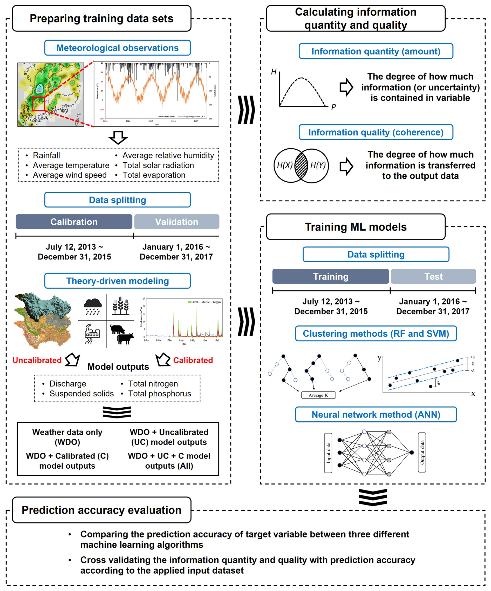
Figure 1 Overall procedure to investigate the contribution of information quantity and quality to the prediction accuracy of hydrological machine learning (ML) modeling.

2 Methods and materials

2.1 Overall procedure

Three ML models, including Random Forest (RF), Support Vector Machine (SVM), and Artificial Neural Network (ANN), were employed in this study (Fig. 1). The ML models were first trained using data sets collected from four study watersheds, including weather data observed at weather stations within or close to the watersheds and flow discharge, SS, TN, and TP measured at the outlets of the four study watersheds. The Soil and Water Assessment Tool (SWAT) model was selected to represent a mechanistic (or theory-driven) model. The SWAT model was used to produce additional data sets to which the ML models would be trained. The SWAT models were calibrated to flow (or streamflow discharges), SS, TN, and TP loads measured at the outlets. Then, the outputs (i.e., flow discharge, SS, TN, and TP loads) of the uncalibrated (i.e., SWAT models with the default parameter values) and calibrated SWAT models were used as additional data sets for the training of the three ML models. Before model training, we carefully separated the ML training and testing datasets to match the SWAT model's calibration and validation periods and to prevent data leakage. For example, we evaluated the ML models using the same validation window used for SWAT, 1 January 2016 to 31 December 2017. Here, we assumed there would be a difference in the quality of information contained in the uncalibrated and calibrated outputs of the SWAT model, and we employed the marginal and transfer entropy based on Shannon's information theory, to quantify the amount and quality of information contained in the training data sets. Finally, the weather data and uncalibrated and calibrated SWAT model outputs were sequentially fed to the three ML models.

Specifically, four datasets were prepared using different types of hydrological data, including weather records and outputs from theory-driven (or mechanistic) models. The first dataset consisted solely of weather data, serving as the baseline. The second and third datasets incorporated uncalibrated and calibrated hydrological model outputs into the baseline, respectively, to evaluate how integrating hydrological knowledge from mechanistic models improves predictions. Additionally, we compared how variations in input data quality influenced model performance. The final dataset combined all input variables, including weather data and both uncalibrated and calibrated model outputs. The baseline model in our study was not intended to replicate a fully developed nutrient model; rather, it was purposefully designed as a foundational benchmark for systematically assessing the effects of incorporating additional information – particularly theory-driven outputs from uncalibrated and calibrated mechanistic models. This framework allowed us to isolate and quantify the incremental gains in ML prediction accuracy as the training data increased in both informational quantity and quality. The use of calibrated mechanistic model outputs as ML training data was a deliberate methodological choice to evaluate how improvements in data reliability influence prediction performance. By excluding nutrient inputs and management practices from the baseline model, we established a consistent reference point for evaluating the added value of such variables when subsequently introduced through mechanistic model outputs. To rigorously assess these effects, we applied Shannon's marginal and transfer entropy to quantify the amount and quality of information embedded in each training dataset. This structured approach enabled a theory-grounded evaluation of how ML model accuracy responds to changes in both data quantity and quality (Fig. 1 and Table 1). Furthermore, we calculated information use efficiency (IUE) to measure how effectively each ML model leveraged added information, based on the improvement in prediction accuracy per unit increase in entropy across the four training data sets.

Table 1 Combinations of data sets used to train hydrological ML models.

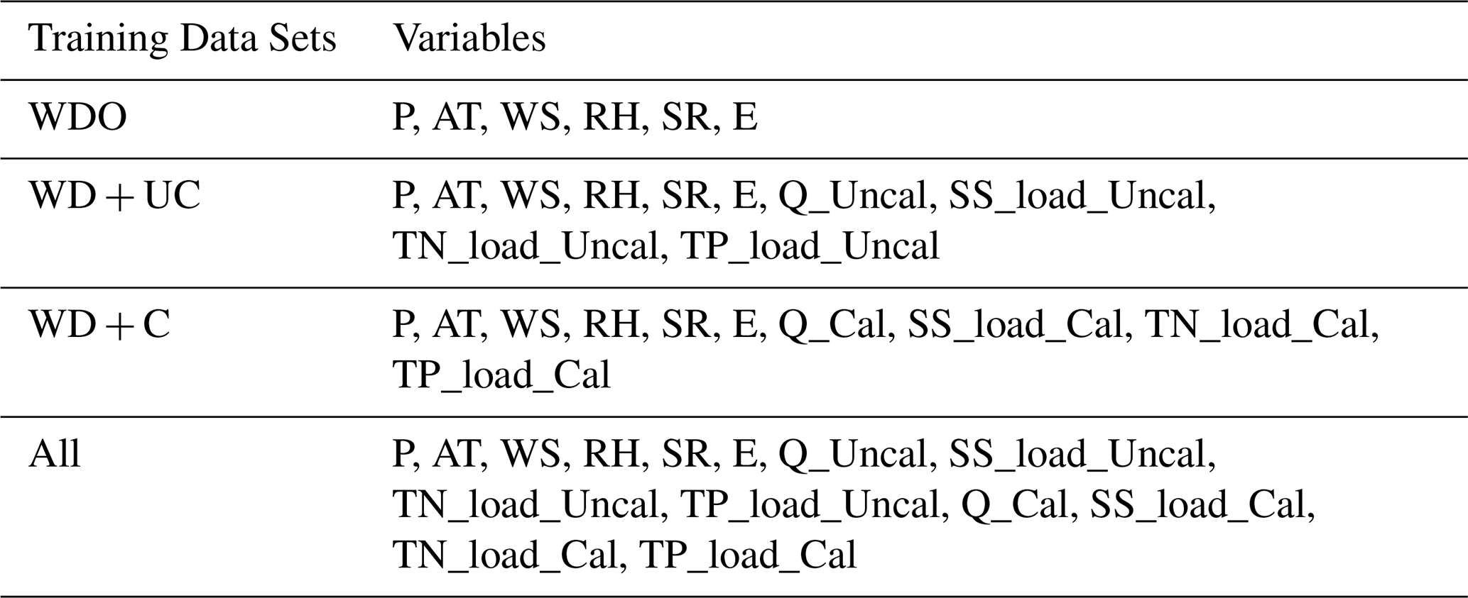
P, AT, WS, RH, SR, and E represent precipitation, average temperature, wind speed, relative humidity, solar radiation, and evaporation, respectively. The SWAT outputs, including Q, SS load, TN load, and TP load, were used to train ML models separately depending on the target variables. For example, SWAT's SS load simulation results were used only when predicting SS load using ML models.

2.2 Data-driven (or machine learning) models

The RF model is based on a regression tree, but it differs as it does not grow with a single tree but rather an entire forest of numerous trees using the bootstrap aggregating technique or bagging technique to help decrease model variance (Breiman et al., 1984; Breiman, 2001). The RF model is known for its ability to be used when there are more variables than observation data, and it does not result in overfitting due to the pruning process (Díaz-Uriate and de Andrés, 2006). The RF model was also reported to offer excellent performance even when predictive variables are irregular (Díaz-Uriate and de Andrés, 2006). In RF modeling, a decision tree grows by splitting a tree node, and it is pruned by removing tree nodes or sections with relatively low explanatory power compared to others (Hasanipanah et al., 2017).

The SVM model divides a high- or infinite-dimensional space using hyperplanes until all data points are separated (Vapnik, 1995, 1998). The SVM model is known to be able to avoid overfitting and produces highly accurate predictions (Aktan, 2011). The goal of the SVM procedures is to identify the optimal hyperplane separating two classes in the high-dimensional space that maximizes the distance between the two data point groups (Ahmed et al., 2017). SVM modeling transforms training data using the kernel function so that a linear hyperplane can separate the data points in high dimensions. Three kernel functions are commonly used: radial basis function (RBF), linear function, and polynomial function. This study employed the RBF, which is the most widely used kernel function (Tao et al., 2008).

The ANN model has been widely used to solve various modeling problems (Khashei and Bijari, 2010). The structure of the ANN model was inspired by the biological structure of the human brain, which is composed of many interconnected processing elements called neurons (Tosun et al., 2016). The structure is characterized by a network of three layers: input, hidden, and output. The number of input and hidden layers is determined by the number of input variables and the complexity of the problem (Yilmazkaya et al., 2018). Neurons are a critical parameter used in interconnected processing, which is characterized by weights (Tosun et al., 2016). The weights of individual neurons determine how input values are transferred to other values on the output nodes. The weights of connections between layers are calculated by the backpropagation process, which calculates the gradient of prediction error with respect to weights (Siddique and Tokhi, 2001).

The optimization of three machine learning models (i.e., RF, SVM, and ANN) was carried out using Bayesian optimization, a method that improves decision-making efficiency by iteratively identifying the most promising hyperparameter configurations (Jones, 2001). Compared to traditional grid or random search methods, Bayesian optimization is notably more efficient in finding optimal hyperparameters (Yu and Zhu, 2020). For the RF model, key parameters such as the maximum number of splits, the number of predictors per split, and the number of trees were optimized. In the case of the SVM model, the kernel scale, epsilon, and cost parameters were fine-tuned. For the ANN model, optimization focused on activation functions and layer sizes. These optimizations were designed to enhance each model's performance by leveraging input variables, including precipitation, temperature, and watershed characteristics that were carefully selected to align with the study's objectives.

2.3 Data normalization and accuracy evaluation

ML modeling is known to have low learning rates when some types of training data have value ranges substantially different from those of others (Ioffe and Szegedy, 2015). Data normalization techniques are commonly used to rescale the training data from their original ranges into a common value range so that the ML models can be efficiently and quickly trained. Several data normalization methods are available; linear scaling is one of the most widely used, presumably due to its simplicity and efficacy (Raju et al., 2020; Eq. 1).

$$\begin{array}{}\text{(1)}& {\mathit{\chi }}^{\prime }=(x-\min (x\left)\right)/\left(\max \right(x)-\min (x\left)\right)\end{array}$$

where χ^′ is the normalized value of the data set (ranges from 0 to 1), and x is an original value.

The prediction accuracy of the three ML models was evaluated using the Kling-Gupta efficiency coefficient (KGE; Gupta et al., 2009). The KGE considers the strength of the correlation between observed and predicted variables while also comparing the variables' biases and variances. Thus, compared to the Nash-Sutcliffe efficiency and the coefficient of determination, the KGE is less sensitive to relatively large values that lead to biases toward such values (Nash and Sutcliffe, 1970; Gupta et al., 2009; Eq. 2).

$$\begin{array}{}\text{(2)}& \text{KGE}=\mathrm{1}-\sqrt{(r-\mathrm{1}{)}^{\mathrm{2}}+{\left({\displaystyle \frac{{\mathit{\sigma }}_{\mathrm{sim}}}{{\mathit{\sigma }}_{\mathrm{obs}}}}-\mathrm{1}\right)}^{\mathrm{2}}+{\left({\displaystyle \frac{{\mathit{\mu }}_{\mathrm{sim}}}{{\mathit{\mu }}_{\mathrm{obs}}}}-\mathrm{1}\right)}^{\mathrm{2}}}\end{array}$$

where σ_obs and σ_sim are the standard deviations of observations and simulation results, respectively, and μ_obs and μ_obs are the averages of observed and simulated variables, respectively.

A KGE of 1 indicates perfect agreement between observations and predictions (Andersson et al., 2017). Knoben et al. (2019) mathematically demonstrated that the KGE value approaches −0.41 when the predicted (or simulated) values of a variable are equal to the average value of its observations. Thus, a KGE value of −0.41 can be interpreted similarly to an NSE value of 0.00, meaning that the predictions may not be a better than the observed mean (Schaefli and Gupta, 2007). In this study, we assumed that predictions would be acceptable or satisfactory when the differences between observed and simulated averages of a variable (or percentage biases) and the variances of the differences are less than 25 % for flow, 55 % for SS, and 70 % for TN $/$ TP (Moriasi et al., 2007), which correspond to KGEs of 0.54, 0.17, and −0.03 for flow, SS, and TN $/$ TP, respectively, with an arbitrarily selected threshold correlation of 0.30.

2.4 Theory-driven (or mechanistic) model

The SWAT model was designed to predict watershed processes based on theories and known mechanisms that control the generation and transport processes of water, sediment, and nutrients (Nietsch et al., 2002). The SWAT model is popularly used to predict water and nutrient loadings at the watershed and basin scales due to its proven applicability to a variety of landscapes and climate zones as well as its simple but defendable modeling strategies. Moreover, the SWAT model can consider various management practices, including application rates and timing of fertilizers and herbicides/pesticides; tillage and low-impact development practices; and agricultural conservation practices such as filter strips, nutrient management plans, terraces, and tile drainage (Her et al., 2017; Her and Jeong, 2018; Li et al., 2021). Several studies have attempted to improve the prediction accuracy of SWAT modeling by coupling it with ML techniques, for example, to predict peak flow (Senent-Aparicio et al., 2019), water quality (Noori et al., 2020), and aquifer vulnerability (Jang et al., 2020).

Two versions of the SWAT model, namely uncalibrated and calibrated mechanistic modeling outputs, were prepared to generate two sets of training data for the ML models. The agricultural management practices, including fertilizer application, planting and harvest dates, compiled from the study watersheds were incorporated into both models (RDA, 2014; Table S2). The values of all parameters of the uncalibrated SWAT model remained unchanged; thus, the uncalibrated SWAT models do not necessarily represent the hydrological processes of the study watersheds, and they are not likely to reproduce the observed flow, SS, TN, and TP at an acceptable accuracy level. Accordingly, the quality of information contained in the outputs of the uncalibrated SWAT models may be relatively low compared to that of the calibrated SWAT models. The parameter values of the SWAT models were calibrated to flow, SS, TN, and TP observations made at the study watersheds' outlets (Table S3). While the SWAT model includes many parameters, previous studies (Arnold et al., 2012; Douglas-Mankin et al., 2010; El-Sadek and Irvem, 2014) have identified key parameters that relatively substantially influence model outputs. In this study, we focused on these parameters for each target variable and calibrated each watershed independently. Calibration was performed sequentially; upstream watersheds were calibrated first, and their calibrated parameter values remained unchanged while calibrating the corresponding parameters for their downstream watersheds. For example, the WJ watershed (which is nested by the HN watershed) was calibrated prior to the HN watershed, and then the parameters for areas that are not included in the WJ watershed but only in the HN watershed were calibrated to observations made at the outlet of the HN watershed. For the target variable, previous studies (Arnold et al., 2012; Engel et al., 2007; Santhi et al., 2001) have recommended that streamflow should be calibrated first, followed by SS, and then TN and TP, due to the interdependencies among these constituents resulting from shared transport processes. The flow, SS, TN, and TP loads predicted using the calibrated SWAT models were assumed to have relatively high-quality information compared to those of the uncalibrated SWAT model. The quantity and quality of information were quantified using the marginal and transfer entropies described in the following section.

The SUFI-2 algorithm, widely used for SWAT model calibration, was used to explore the multi-dimensional parameter spaces of the SWAT models and locate a solution (or a parameter set) close to the global optimum in this study (Sao et al., 2020). The simulation period was split into three: a warm-up period from 1 January 2008 to 11 July 2013; a calibration period from 12 July 2013 to 31 December 2015; and a validation period from 1 January 2016 to 31 December 2017. The types and value ranges of the calibration parameters were determined based on the previous SWAT modeling experience, the understanding of the calibration parameters, and the literature (Tobin and Bennett, 2017; Tang et al., 2021).

2.5 Marginal and transfer entropy

This study measured the quantity and quality of information contained in the training data using marginal and transfer entropies. In general, a data set that is spread out has relatively high entropy, while another data set that is concentrated on a small range of values has relatively small entropy. The marginal entropy is defined as the information content of a variable and used to calculate randomness in time series using Eq. (3) (Shannon, 1948; Cover and Thomas, 2006; Silva et al., 2017):

$$\begin{array}{}\text{(3)}& H\left(X\right)=-\sum _{i=\mathrm{1}}^{n}p\left(x_i\right){\log }_{\mathrm{2}}P\left(x_i\right)\end{array}$$

where H(X) is a measure of information of a discrete random variable X, and P(x) is the probability mass function of variable x in the ith step. The base-2 logarithm is used in the entropy calculation to express information content in bits (Shannon, 1948).

While the amount of information contained in a variable can be calculated using the marginal entropy, we can also calculate the amount of information shared between two variables based on mutual information theory using Eq. (4) (Cover and Thomas, 2006):

$$\begin{array}{}\text{(4)}& I\left(X;Y\right)=H\left(X\right)+H\left(Y\right)-H\left(X,Y\right)\end{array}$$

where I(XY) is the quantified value between X and Y. The mutual information I(XY) represents the expected information gained in Y from measuring X, or vice versa. From these definitions, we can calculate the conditional entropy by subtracting the amount of information shared between X and Y from H(X), which indicates how much information remains about the entire time series X in case we already know the information content of Y.

$$\begin{array}{}\text{(5)}& H\left(X\left|Y\right.\right)=H\left(X\right)-I\left(X;Y\right)\end{array}$$

These quantities are all symmetrical and do not explain the amount of information exchanged between variables (Bennett et al., 2019). The transfer entropy was devised to consider the asymmetric transfer of information between any two-time series X and Y (the information flow from one to another variable), and can be defined as conditional mutual information (Schreiber, 2000):

$$\begin{array}{}\text{(6)}& T_{X\to Y}=I(Y_t;X_t\left|Y_t\right.)\end{array}$$

where T_X→Y is the transfer entropy from X to Y, and X_t or Y_t denotes the variables X and Y in time t. The lag parameter, which defines the time delay between variables X and Y, was set to zero because the ML models used in this study are standard regression models without explicit temporal memory (e.g., no long-short term memory model); accordingly, we quantified synchronous information-use between inputs and outputs (i.e., the lag time or time delay between X and Y is zero), which aligns with our primary objective.

Transfer entropy was calculated using a quantile-based discretization scheme provided by the RTransferEntropy package (Behrendt et al., 2019) for R software. This method enhances robustness to outliers and better captures information transfer associated with relatively high and low values (Nie, 2021; Zhang and Zhao, 2022). Once the marginal and transfer entropies were calculated for the modeling experiments with the unique combinations of the ML models and the training data sets (Fig. 1 and Table 1), the prediction accuracy gain was divided by the increases in the quantity (marginal entropy) and quality (transfer entropy) of information contained in the training data to calculate IUE:

$$\begin{array}{}\text{(7)}& {\displaystyle }{\mathrm{IUE}}_{\mathrm{ME}}={\displaystyle \frac{P_{\mathrm{WD}\to \mathrm{ID}}}{\sum H(x_{\mathrm{WD}}\to x_{\mathrm{ID}})}}\text{(8)}& {\displaystyle }{\mathrm{IUE}}_{\mathrm{TE}}={\displaystyle \frac{P_{\mathrm{WD}\to \mathrm{ID}}}{\sum T_{{\mathrm{WD}}_i\to Y}\to \sum T_{{\mathrm{ID}}_i\to Y}}}\end{array}$$

where P_WD→ID is the prediction accuracy gain or increase from using additional straining data sets, as compared to the case of only using weather data for the training. The H(x_WD→x_ID) and $\sum T_{{\mathrm{WD}}_i\to Y}\to \sum T_{{\mathrm{ID}}_i\to Y}$ denotes the marginal entropy and transfer entropy gain or increase from using additional straining data sets, compared to the case of only using weather data for the training.

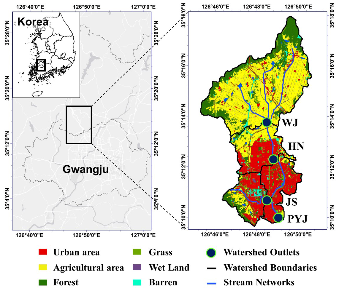
Figure 2 Location of the study watersheds and their land uses and covers.

2.6 Study watersheds and training data acquisition

The Pung-Yeong-Jung (PYJ) river watershed was selected for the modeling experiment of this study. The PYJ watershed can be divided into three sub-watersheds from upstream to downstream: the Wall-Jeong (WJ), Ha-Nam (HN), and Jang-Su (JS) watersheds (Fig. 2 and Table S1 in the Supplement). The WJ watershed is nested by the HN watershed, and the HN and JS watersheds are nested by the PYJ watershed. Thus, all direct runoff drained from the three nested watersheds passes the outlet (35°09^′58.87^′′ N, 126°49^′08.93^′′ E) of the PYJ watershed. The streamflow, SS, TN, and TP concentrations were monitored at the outlets of the four study watersheds for four years and six months, from 12 July 2013 to 31 December 2017. Most of the drainage areas were covered by agricultural land uses, including upland and rice paddy fields (covering 41 % of the JS watershed and 62 % of the WJ watershed) and forest. Urbanized areas cover 5 % (WJ watershed) to 31 % (JS watershed) of the watersheds.

Streamflow, SS, TN, and TP concentrations were monitored at the outlets of the four study watersheds over a period of four years and six months, from 12 July 2013 to 31 December 2017. These monitoring data were divided into two non-overlapping subsets: one for model training and the other for testing. To prevent potential data leakage, we applied a consistent temporal split such that the training and testing periods for the ML models matched the calibration and validation periods of the mechanistic model (i.e., SWAT), respectively. In this setup, the three ML models were trained on data corresponding to the SWAT model calibration period (12 July 2013 to 31 December 2015), while their prediction accuracy of the ML models was evaluated using the testing dataset from the SWAT validation period (1 January 2016 to 31 December 2017), ensuring a clear separation between the data used for model training and for model evaluation (Fig. 1). To ensure the integrity of the experiment, observed discharge and concentration data were used solely for the calibration and validation of the SWAT model and were not reused in training the ML models. This separation of data sources was a deliberate aspect of the study design to maintain the independence of the ML training process and to avoid any unintended data leakage.

The Korean Meteorological Administration monitors weather variables, including daily AT, P, E, WS, RH, and SR, at a weather station located approximately 7 km away from the study watersheds. Water pressure sensors and data loggers (OTT Orpheus Mini, Germany) were deployed at the monitoring sites close to the watershed outlets. The cross-sections of the streams were surveyed at the monitoring sites, and the velocity of streamflow was then measured using a flow meter (VALEPORT model 002, UK) across the sections to estimate flow discharge rates. Water quality samples were manually collected every one or two weeks. During a rainfall event, stream water was collected using an automatic sampler (ISCO portable sampler 6712, USA), and the sampling interval was reduced to 1 h to catch the expected large variations of flow rates and the corresponding water quality concentrations for improved observation accuracy. During the monitoring period, a total of 17 large rainfall events were sampled.

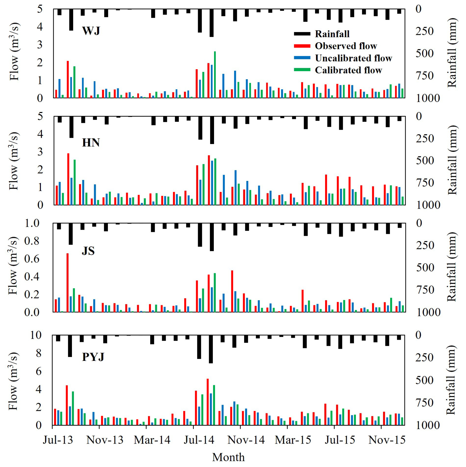
Figure 3 Comparison of monthly streamflow predicted using the mechanistic models (i.e., uncalibrated and calibrated SWAT models) and observed during the training period (12 July 2013 to 31 December 2015). The daily-scale comparisons can be found in the Supplement (Figs. S1–S4).

3 Results

3.1 Training data: Weather records and monitoring data

Sets of training data were prepared using the daily weather records, the watershed monitoring data, and SWAT modeling results (uncalibrated and calibrated outputs; Figs. 3 and S1–S4). The watersheds have four seasons, with relatively short springs and falls. The watersheds are fairly wet in the summer and dry in the spring. For example, the watersheds receive precipitation of 831–1333 mm annually, with more than half (59 % on average) of the precipitation occurring in the summer (from June to September). In spring, the stream might dry up due to the small amount of precipitation and warm air. In the case of the PYJ watershed, streamflow discharges can be large, with as much as 2.64 m³ s⁻¹ on average in summer, but they are limited (e.g., 1.21 m³ s⁻¹) enough to reveal the bottom of the stream in spring (from March to May).

The PYJ and JS watersheds had the largest and smallest average daily discharge of 1.69 and 0.16 m³ s⁻¹, respectively (Table S4). The JS watershed had relatively higher SS concentrations compared to the other watersheds as it includes large construction sites (Adeola-Fashae et al., 2019; Mendie, 2005; Pullanikkatil et al., 2015). In addition, the first flush effects of the urbanized watersheds (e.g., the JS watershed; Table S1) led to higher peak SS, TN, and TP concentrations (Chaudhary et al., 2022). The WJ and HN watersheds had relatively higher TN and TP concentrations, presumably due to agricultural management activities such as fertilizer application and livestock farming in their large agricultural areas (Liu et al., 2012; Table S4).

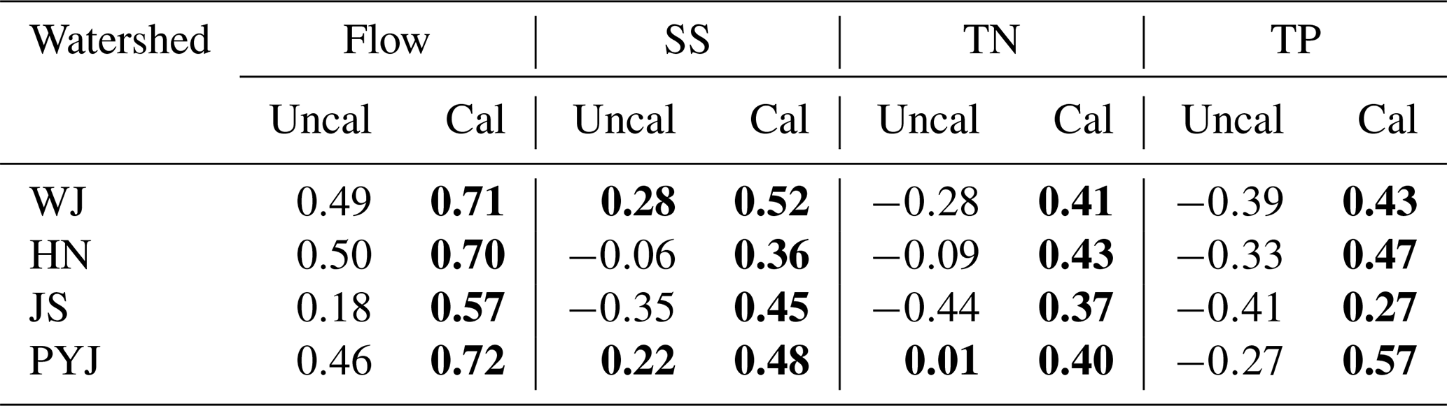
Table 2 Accuracy statistics (KGEs) of a theory-driven (or SWAT) model in the training period. The KGE scores that satisfy the acceptable accuracy criteria (i.e., 0.54 for flow, 0.17 for SS, −0.03 for TN $/$ TP) are in bold.

3.2 Training data: Outputs of the mechanistic modeling

The calibrated SWAT model provided acceptable performance in all watersheds (e.g., KGEs equal to or greater than 0.54 for flow, 0.17 for SS, and −0.03 for TN $/$ TP). The average KGE values for all watersheds were 0.68 for flow, 0.45 for SS, 0.40 for TN, and 0.44 for TP (Table 2). However, as expected, the uncalibrated model could not accurately predict the variables; average KGEs for all watersheds were less than 0.41 for flow, 0.02 for SS, −0.20 for TN, and −0.35 for TP. As such, the information quality of the outputs of the calibrated SWAT modeling may be greater than that of the uncalibrated modeling. The quantity and quality of information were evaluated with marginal and transfer entropies.

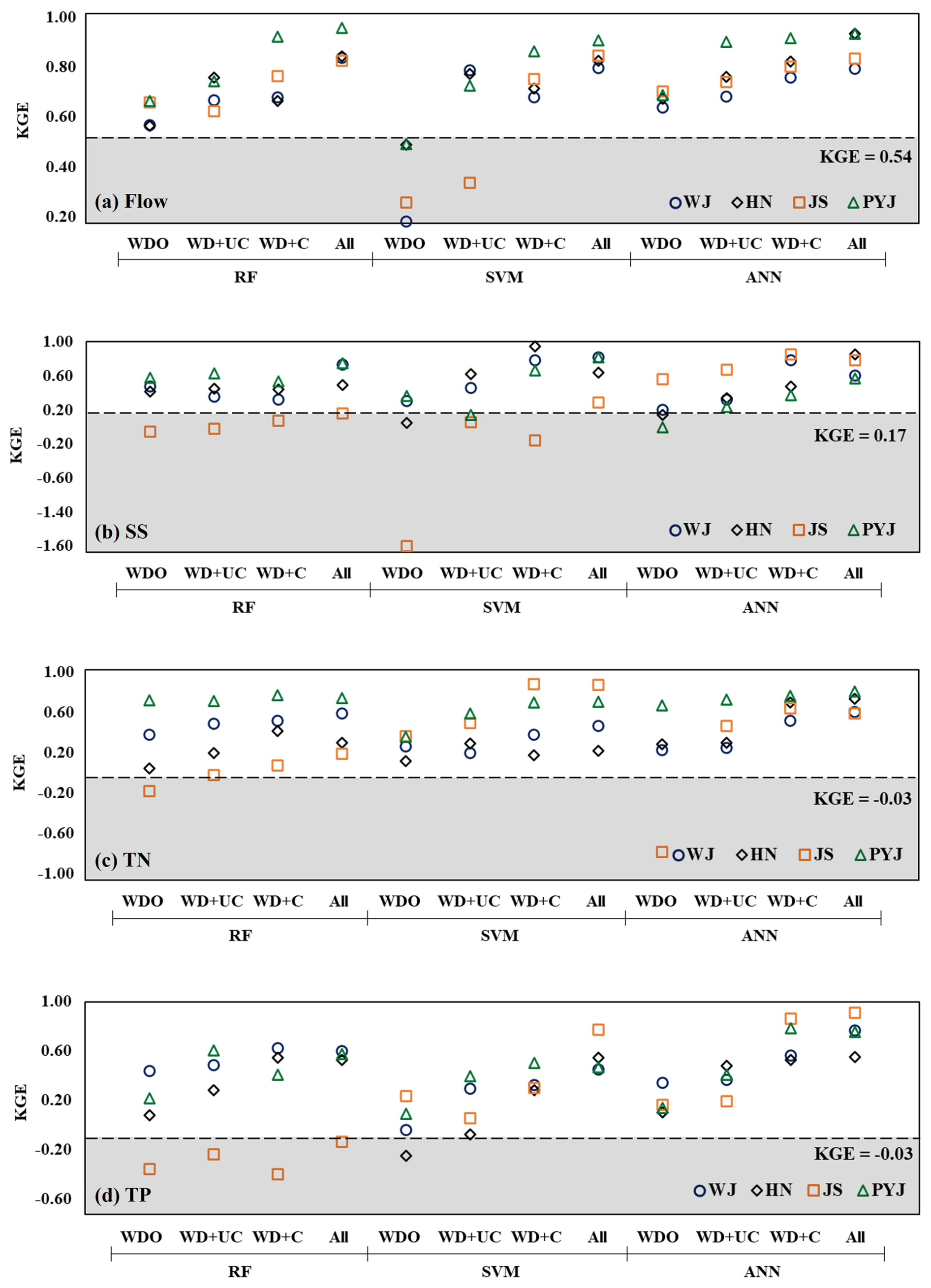
Figure 4 Prediction accuracy (KGE) of hydrological ML models trained with the different training data set combinations. The KGE values that do not satisfy the acceptable accuracy levels (e.g., i.e., 0.54 for flow, 0.17 for SS, and −0.03 for TN $/$ TP) are included in gray areas.

3.3 Prediction accuracy of machine learning modeling

The four ML models were trained with different sets of training data: weather data only (WDO), the uncalibrated SWAT modeling outputs added to WDO (WD + UC), the calibrated SWAT modeling outputs added to WDO (WD + C), and all training data (All or WD + UC + C). The trained ML models yielded unique performances in the predictions depending on the training data set types (Fig. 4). Overall, the ML models' prediction accuracy consistently improved as additional data sets were added to the training data, including WDO to WD + UC, WDO + C, and All (Fig. S5a). For example, the WDO case provided acceptable accuracy (KGE of 0.67 greater than the threshold of 0.54) in the prediction of flow using the RF algorithm at the outlet of the PYJ watershed. When the outputs of the uncalibrated and/or calibrated SWAT modeling were added to the training data, the accuracy of the ML modeling was increased to KGEs of 0.74 (11.6 % increase with WD + UC) and 0.91 (37.2 % increase with WD + C) in the case of using the RF model. The additional training data sets also improved the accuracy of the water quality ML modeling. However, ML models trained only using the weather data and uncalibrated mechanistic modeling outputs failed to meet the acceptable accuracy levels (i.e., 0.17 for SS and −0.03 for TN $/$ TP; Fig. 4). In Fig. 4, the KGE scores overall increase from left to right. Negative KGE scores are frequently found in the JS watershed, indicating the models relatively poorly performed for the watershed.

None of the ML models consistently provided more accurate predictions than the others (Figs. 4 and S5b). This finding aligns with other studies that identified no ML model that is universally applicable to all data sets or problems (Alzubi et al., 2018; Domingos, 2012). A study has demonstrated that the RF model is more accurate compared to the SVM and ANN models (Al-Mukhtar, 2019). Conversely, another study has determined that the SVM or ANN model outperform the RF model (Ahmad et al., 2018). In this study, the RF model provided relatively better accuracy than other ML models when predicting the streamflow of the PYJ watershed using all training data sets (the All case). The ANN model was the only one that could provide acceptable accuracy (KGE of 0.84, which is greater than the threshold of 0.17 for SS) in the prediction of SS loads in the JS watershed with the WD + C training data. The SVM model provided a relatively greater KGE score than the other models when predicting the SS loads of the HN watersheds using the WD + UC training data.

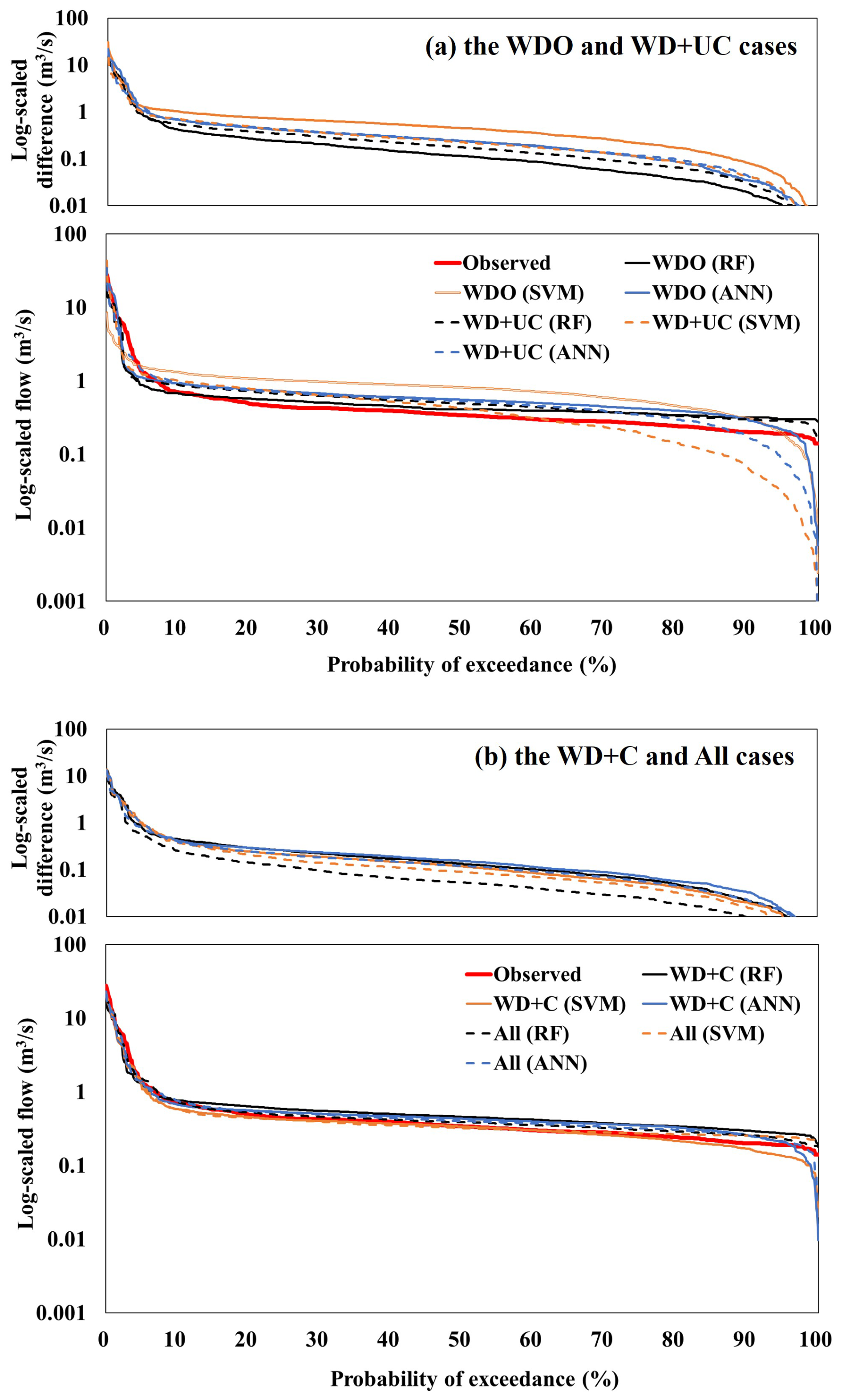
Figure 5 Comparison between observed and ML-predicted FDCs at the outlet of the WJ watershed.

A flow duration curve (FDC) provides a graphical way of investigating the frequency of extreme events, such as floods and droughts. The FDCs were derived from the observed and predicted flow hydrographs and compared to evaluate prediction accuracy in the frequency domain (Figs. 5 and S6). The FDCs created from flow predictions made using the ML models trained with all training data (the All case) were the closest to the observed FDC in both high (e.g., flooding) and low (e.g., drought) exceedance probability regions. The WDO and WD + UC cases created relatively large differences (under- and over-estimations) between the predicted and observed FDCs, especially for extreme events (i.e., flooding and drought). For example, the differences between the ANN predictions and observations for the 5 % (flooding) and 95 % (drought) exceedance probabilities of the WJ watershed were 18.1 % and 13.8 % in the All case respectively, and they increased to 28.8 % and 77.9 % in the WD + UC case. The findings indicate that the ML models trained with all available training data sets (the All case) can more accurately predict the extremes than the relatively less trained ML models (the WDO and WD + UC cases).

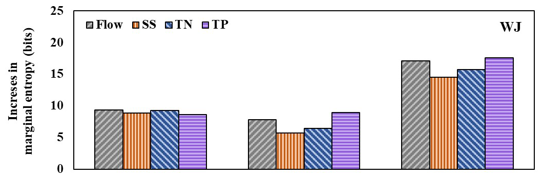
Figure 6 Increases in marginal entropy due to the addition of additional training data sets in the case of the WJ watershed. The WDO training data set serves as the baseline for this comparison.

3.4 Information quantity and quality

The amount and quality of information contained in the training data sets for the ML training were quantified using the marginal and transfer entropy concepts, respectively. Then, IUE scores were calculated to understand how efficiently information quantity and quality can improve the prediction accuracy of hydrological ML modeling. marginal entropy of the training data sets generally increased as additional data (i.e., the outputs of the uncalibrated and calibrated mechanistic or SWAT modeling) were added to the weather data (i.e., WDO case; Figs. 6 and S7–S8). In the case of predicting the flow of the WJ watershed, for example, marginal entropy increased by 7.8 to 17.1 bits when the uncalibrated and/or calibrated SWAT modeling outputs were added to the training data respectively, compared to the WDO case (Fig. 6). The All cases increased marginal entropy more substantially than the WD + UC and WD + C cases, regardless of the watersheds and variables. The WD + C cases did not always increase marginal entropy more than the WD + UC cases, and the marginal entropy increases were negligible even when they did occur (e.g., in the case of predicting TP loads); this confirms that marginal entropy does not consider the association between two variables (i.e., watershed responses observed and simulated using the calibrated mechanistic models) in the training data sets, which is one of the features that marginal entropy has. Thus, marginal entropy does not change depending on the types of ML models as marginal entropy only counts information in the training data.

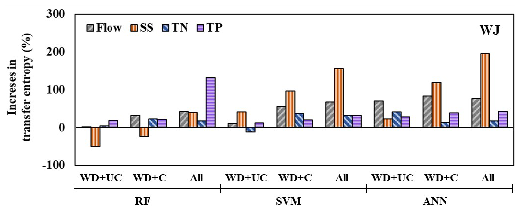
Figure 7 Increases in transfer entropy due to the addition of training data sets in the case of the WJ watershed. The WDO training data set serves as the baseline for this comparison.

Transfer entropy did not always increase with additional training data (Figs. 7 and S9, Table S6). For example, in the case of the RF modeling trained with the WDO data set for the WJ watershed, the transfer entropy of SS loads decreased from 0.385 to 0.190 and 0.294 when adding uncalibrated and calibrated mechanistic modeling outputs, respectively (Fig. 7); this indicates that a loss of information was commonly found in the target and training data sets when adding additional data, such as uncalibrated and calibrated modeling outputs, to the training data set. The amount of precipitation information (0.174 bits) was transferred to the SS prediction for the WJ watershed in the case of WDO. However, when adding the uncalibrated mechanistic (i.e., SWAT) modeling output to the training data set, the amount of transferred precipitation information decreased to 0.066 bits, whereas only 0.044 bits were transferred from the uncalibrated SWAT modeling output. Here, the information loss of 0.064 bits can be calculated by subtracting 0.110 bits (amount of information on precipitation and uncalibrated mechanistic modeling output when applying WD + UC training data set) from 0.174 bits. Transfer entropy quantifies the amount of information contained in the training data sets that is effectively transferred into the predictions made using the trained ML models. It captures not only the shared information between input and output variables but also the directional flow of information from one variable to another (Schreiber, 2000). Thus, transfer entropy depends on the types of training data sets, prediction variables, and ML models (Fig. S8 vs. S10).

3.5 Information use efficiency

The IUE represents the relative improvement of prediction accuracy compared to the baseline per unit change of information quantity (Eqs. 7 and 8). IUE was calculated by dividing the increases in KGEs (the WDO training data set serves as the baseline) by the differences between the amount of information quantified using marginal entropy (IUE-ME) or transfer entropy (IUE-TE) contained in the training data sets (Fig. 8).

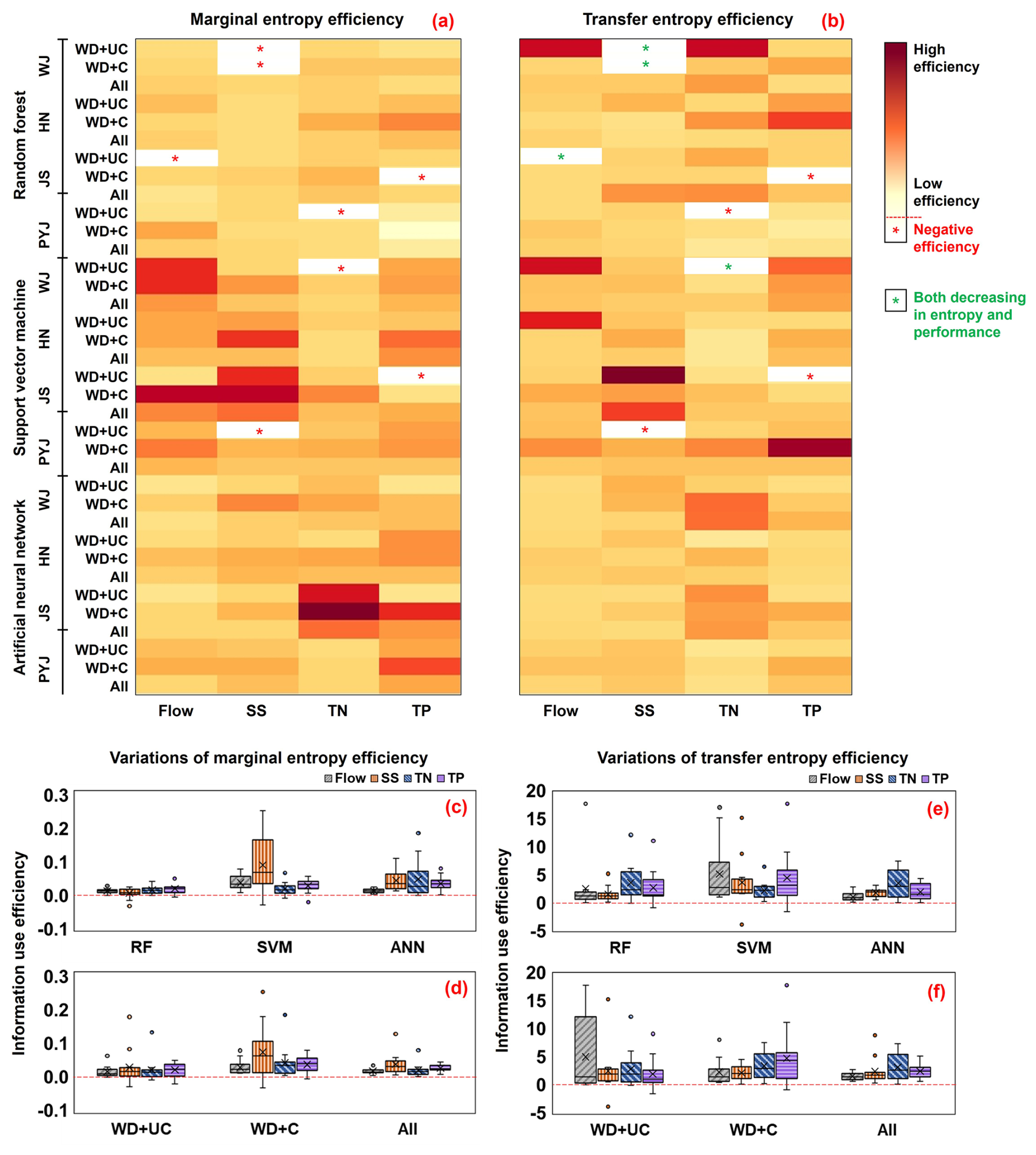
Figure 8 Comparison of changes in information use efficiency (IUE) calculated from the entropy (marginal and transfer entropies) and accuracy (KGE) statistics provided by using the different training sets. (a) and (b) exhibit relative changes in information use efficiency (IUE-ME and IUE-TE) across all factors, including the ML models, watersheds, training datasets, and predicted variables. Red asterisks marks represent “Negative efficiency” describing the case where prediction accuracy decreased with increases in entropy, and green asterisks marks indicate the cases where both IUE and KGE decrease. (c) and (d) summarize, with box-whisker plots, the variations of changes in IUE-ME for the watersheds and training datasets (c) and for the watersheds and ML models (d), respectively; (e) and (f) show the variations of changes in IUE-TE for the watersheds and training datasets (e) and for the watersheds and ML models (f), respectively.

The case of WD + C provided a relatively higher IUE-ME compared to the other training data cases (Fig. 8d and Table S5). This means that the prediction accuracy of ML modeling can be most efficiently improved when the outputs of the calibrated mechanistic modeling are added to the training data sets (i.e., WD + C). Interestingly, WD + C may be more efficient than the All case, which added the uncalibrated theory-driven modeling outputs to WD + C. This finding implies that information quality can more efficiently improve the prediction accuracy of hydrological ML modeling than information quantity. However, it is worth noting that the All case still provided the best prediction accuracy (or the highest KGE), but its IUE in increasing KGE scores was lower than that of WD + C when considering the relative accuracy improvement to the amount of added information.

IUE-ME were often negative, especially in the WD + UC case, indicating that prediction accuracy decreased even when entropy increased (red star in Fig. 8a); this is because marginal entropy always increases with additional input variables, regardless of their quality or association with the target variables. IUE-TE also showed negative efficiency, which means the KGE decreased with increases in the transfer entropy. Model performance might not necessarily relate to transfer entropy because of complicated associations among weather forcings, management practices, watershed feathers, and responses (Konapala et al., 2020). KGEs also decreased when transfer entropy decreased (green star in Fig. 8b), which implies that transfer entropy can capture the decrease in information flow between independent (i.e., weather data, uncalibrated and calibrated modeling outputs) and dependent (or target) variables that may lead to decreased prediction accuracy (or decreased KGEs). This inverse relationship was primarily detected when adding uncalibrated mechanistic modeling outputs to the training data set, demonstrating the role of information quality in ML modeling training.

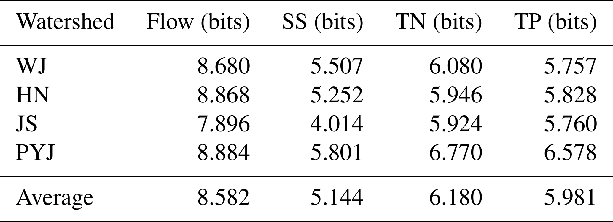
Table 3 Marginal entropy quantified for target variables observed at the watershed outlets in the training period.

4 Discussions

4.1 Influence of target variables and watershed characteristics on ML performance

The prediction accuracy of the ML models varied according to the variables of interest (flow, SS, TN, and TP). The RF, SVM, and ANN ML models were best at predicting the flow of the study watersheds compared to the other variables (Figs. 4 and S5). For example, the ML models provided KGEs of 0.557 (WDO) to 0.854 (All) when predicting flow versus KGEs of 0.093 (WDO) to 0.607 (All) for SS loads. This variance is presumably because of the previously described differences in the amount of information contained in the watershed responses or target variables. For example, the flow hydrographs commonly have relatively higher marginal entropies (8.582 on average) than the other variables' hydrographs (5.144 for SS, 6.180 for TN, and 5.981 for TP on average) for all study watersheds (Table 3). In the frequency domain, normalized SS load data have the most biased distributions toward low values (small SS loads) and the highest frequencies among the watershed responses or target variables, leading to relatively low entropy in the SS data (Fig. S11). The SS, TN, and TP concentrations observed at the watershed outlets have relatively small variations compared to the flow (Table S4), which might be attributed to the fact that water quality variables were much less frequently measured (or sampled) than flow (Table S4, the number of observations); thus, potentially large concentration variations might not be apparent in the observations. These comparison results imply that the frequency of water quality sampling can affect the amount of information in training data and the accuracy of hydrological ML model prediction.

The accuracy of the ML modeling also varied by the watersheds. Regardless of the training data sets, the ML models provided the best prediction accuracy for the PYJ watershed, which has the largest drainage area, while they did the worst for the JS watershed, which has the smallest drainage area; this implies the potential impact of watershed features and responses (flow, SS, TN, and TP) on ML prediction accuracy. For example, entropy in the watershed responses of the PYJ watershed was consistently higher than that of the JS watershed (Table 3). In the case of WDO, the amount of information contained in the independent variables (i.e., only weather records observed at a single station) of the training data set should be the same for the PYJ and JS watersheds. However, their responses (dependent or target variables) differ and thus have different entropy (or information) scores. The responses of the PYJ watershed are spread out over wide value ranges, which means relatively high entropies compared to those of the other watersheds, especially the JS watershed (Fig. S11). The flow observed at the outlet of the JS watershed are relatively highly biases toward low flow ranges. ML model prediction accuracy was found to be associated with the entropy in the watershed responses (Fig. 9). The results indicated that the KGE (i.e., prediction accuracy) scores of the ML models generally increased with increases in the amount of information contained in the target variables (Fig. 9).

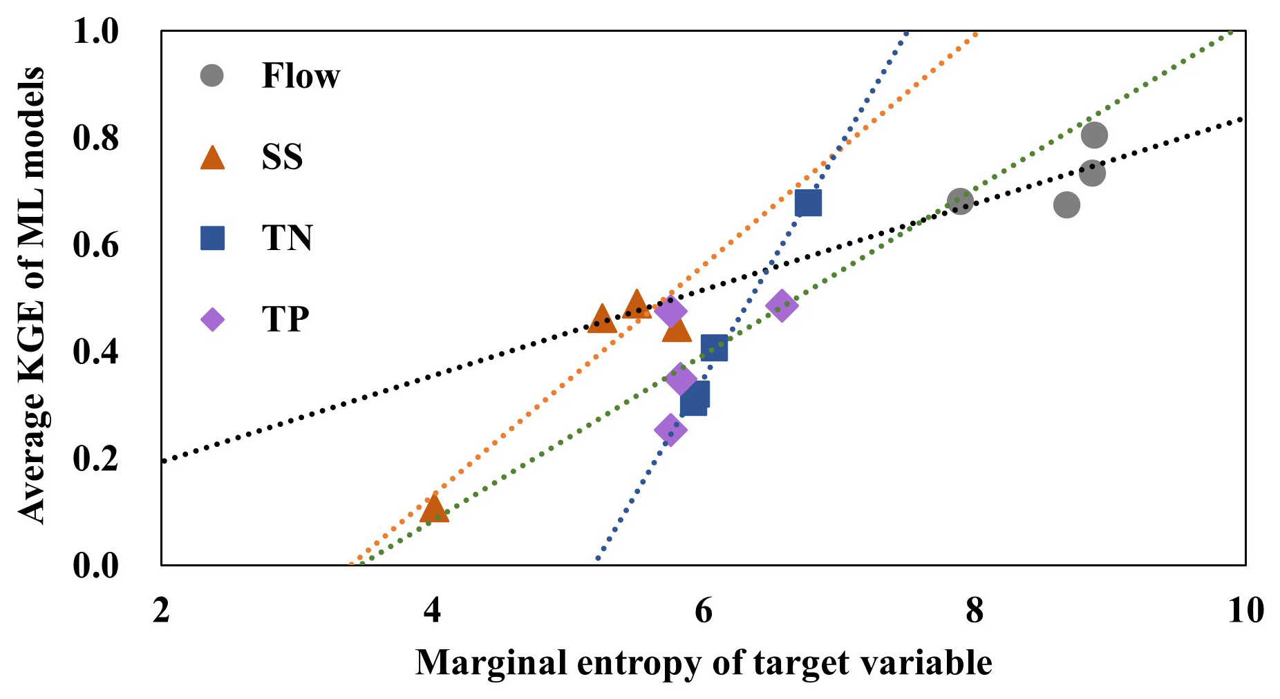
Figure 9 Linear relationship between the average KGE scores of three ML models trained using the four training data sets and the marginal entropy of the target variables.

4.2 Influence of model structure on ML performance across information quantity and quality

Despite being trained on identical datasets, ML models exhibited different predictive abilities in response to increases in information quantity and quality. The ANN and SVM models could improve their predictions more efficiently in terms of the amount of information (i.e., marginal entropy) added to the training data compared to the RF model (Fig. 8c). The RF model uses a random sampling method to select the feature subspace for each node in growing the trees (Breiman, 2001), which is a model parameter called the “number of variables”. Previous studies (Wang and Xia, 2016; Ye et al., 2013) have argued that when applying the random sampling method to a high-dimension data set, model may select many subspaces that do not include informative features and will increase error bounds for the RF model. This study agrees with previous studies: RF performed relatively poorly when dimension of a training data set was higher (i.e., the large number of independent variables) than SVM and ANN. A traditional ANN model with one or two hidden layers is known to suffer performance degradation due to its rapid growth in the number of connection weights (Krenker et al., 2011). However, one study demonstrated that a deep neural network that employs numerous hidden layers, such as the one used in this study, could yield promising performance with high-dimensional training data (Liu et al., 2017).

In addition, negative IUE-TE values were observed when watershed responses were predicted using RF and SVM models (red star in Fig. 8b), particularly in the WD + UC case, suggesting challenges in leveraging additional information from training data. While SVM models use kernel function to transform non-linear decision spaces into linear ones, and RF models employ non-linear decision boundaries, prior studies indicate that such methods are not always effective in resolving high-dimensionality issues, often sampling less informative features (Wang and Xia, 2016; Ye et al., 2013). Despite the radial basis kernel function and Bayesian optimization employed in this study to enhance SVM performance (Shawe-Taylor and Sun, 2011), the model's predictive accuracy remained inconsistent. Conversely, the ANN model avoided negative IUE scores, demonstrating its robustness by effectively exploiting additional information even when lower-quality data (WD + UC) were added to the training dataset (Fig. 8b and e). This indicates that the ANN model excels at handling high-dimensional, non-linear data, making it more effective than RF and SVM for this study's hydrological predictions. With diverse features such as precipitation, temperature, and watershed characteristics contributing to accurate predictions, the ANN model utilized the rich, high-dimensional data from calibrated and uncalibrated SWAT outputs to achieve strong performance. Unlike clustering methods, which primarily group data without a predictive function, neural networks improve prediction accuracy through learning from labelled data and adapting to input quality. The absence of negative IUE scores for ANN underscores its flexibility and robustness. These findings affirm the ANN model's suitability for high-dimensional hydrological modeling, highlighting its advantage over other methods in tasks requiring predictive precision and adaptability to data complexity.

4.3 Implications, limitations, and future directions for integrating ML with mechanistic models

The quantitative evaluation of data quality and quantity in relation to model performance provides actionable insights for future modeling efforts. Our findings highlight the importance of prioritizing high-quality, high-relevance inputs to improve prediction accuracy. This suggests feature selection techniques, informed by our results, could help identify the most impactful variables, reducing the risk of overfitting and computational inefficiencies. The demonstrated sensitivity of ML models to data quality suggests the need for rigorous preprocessing steps, such as outlier detection, imputation of missing data, and validation of sensor measurements. For example, ensuring consistent and accurate data collection at critical watershed locations can enhance model reliability. Our results could guide the development of benchmarks or thresholds for data quality metrics (e.g., measurement error limits) to ensure datasets meet the minimum requirements for effective modeling.

Our findings also have implications for hybrid modeling approaches, particularly guiding the integration of ML with mechanistic models. These results can help select variables where mechanistic models provide better physical realism (e.g., water and nutrient transport) while leveraging ML for complementary predictions (e.g., extreme event responses or data gap interpolation). Improving the quality of key inputs can also help reconcile discrepancies between data-driven and theory-driven predictions, enhancing overall model accuracy. Expanding beyond standalone ML applications, this study provides a foundation for adaptive modeling frameworks that dynamically assess and adjust data inputs based on their predictive contributions.

Future studies could build on our quantitative evaluation by applying these insights to develop guidelines or workflows for selecting and preparing datasets tailored to specific hydrological and water quality objectives. The study underscores the need to refine hydrological ML prediction models by emphasizing the connection between training data quantity, quality, and prediction accuracy. These results suggest that higher-quality training data improved the IUE of ML models, enabling them to maintain or improve prediction accuracy while using a reduced number of inputs. The integration of theory-driven and data-driven approaches will not only improve prediction accuracy but also streamline model training by ensuring that the data used contains both sufficient quantity and quality. Moreover, a deeper understanding of the interaction between different data types will inform more effective training strategies for ML models, leading to more accurate and reliable hydrological predictions.

While this study provides valuable insights into the relationship between ML prediction accuracy and the quality and quantity of input data in hydrological modeling, several limitations and uncertainties must be acknowledged. The study's findings are based on a specific set of watersheds with unique hydrological, climatic, and geographical characteristics. The variability in watershed conditions across different regions may limit the generalizability of the results. The study assumes that the available datasets accurately represent real-world hydrological processes. However, biases, errors, and inconsistencies in the input data, such as measurement inaccuracies or missing values, could influence the results. The study evaluates model performance at specific temporal and spatial scales. Fine temporal resolutions (e.g., daily predictions) may introduce additional complexities not captured in coarser scales (e.g., monthly or annual). Despite optimization efforts, ML models remain susceptible to overfitting, particularly when trained on small datasets or when irrelevant features are included. By acknowledging these limitations and uncertainties, this study provides a helpful starting point for future work to build upon, with the goal of enhancing the reliability of ML models in hydrological applications.

5 Conclusions

This study provides clear evidence that the predictive accuracy of hydrological ML models is intricately linked to both the quantity and the quality of information embedded within the training datasets. The highest overall accuracy was achieved when the full suite of available data sources was used to train the models (i.e., the All case). However, the most efficient improvements in predictive accuracy – relative to the amount of information added – were realized when high-quality outputs from calibrated mechanistic models were incorporated (i.e., the WD + C case).

To better characterize the nature of these improvements, we employed metrics from information theory, specifically marginal entropy and transfer entropy, to quantify the amount and relevance of information in each training dataset. Furthermore, we introduced IUE as a novel indicator to evaluate how effectively additional information contributes to gains in prediction accuracy.

The findings underscore the critical role of information quality in hydrological ML modeling. In particular, augmenting training datasets with low-relevance or low-accuracy data (as in the WD + UC case) did not necessarily improve – and in some cases degraded – model performance. This highlights the potential risks associated with increasing data volume without due consideration of informational relevance.

Importantly, the combined application of marginal entropy, transfer entropy, and IUE offers a robust and interpretable framework for evaluating and optimizing training data. These metrics facilitate a more rigorous assessment of how data characteristics influence model performance, providing actionable insights for both model development and data acquisition strategies. By leveraging this framework, hydrologists and modelers can more effectively select and structure training datasets that balance both informational quantity and quality, ultimately improving the robustness and generalizability of hydrological ML predictions.