Catchment transit time variability with different SAS function parameterizations for the unsaturated zone and groundwater

Preferential flow paths (e.g., macropores or subsurface pipe networks) in hydrological systems facilitate the rapid transmission of precipitation and solutes to streams, resulting in streamflow responses characterized by the release of younger water (i.e., recent precipitation) from the catchment and correspondingly short transit times (on the order of days). While preferential flow paths are documented in both the unsaturated zone and groundwater aquifers, it remains uncertain whether catchment-scale isotope-based transport models can adequately represent preferential flow using tracer measurements in streamflow. In this study, we hypothesize that the preferential release of young water from both the unsaturated zone and groundwater aquifers can be isolated from the streamflow tracer signal. This can be studied with StorAge Selection (SAS) functions, which describe how young or old water leaves a storage. We systematically compared multiple parameterizations of SAS functions describing how water of different ages is released from the unsaturated zone and groundwater aquifer within a single catchment-scale transport model using long-term measurements of hydrogen isotopes in water (δ²H) from two headwater catchments (the Hydrological Open Air Laboratory (HOAL) in Austria and the Wüstebach catchment in Germany). The results show that δ²H measurements in streamflow exhibited sufficient variability to isolate the preferential release of younger water through preferential flow paths in the unsaturated zone. In contrast, the variability of δ²H in streamflow was insufficient to isolate the preferential release of younger water from the groundwater aquifer, as any seasonal variations in pore water δ²H were largely damped by substantial passive groundwater storage (water that mixes with the tracer signal of the active groundwater volume). Consistent with this interpretation, the degree of attenuation in the simulated streamflow isotope signal increased with increasing passive groundwater storage volumes and became pronounced when passive storage was orders of magnitude larger than active groundwater storage. The size of passive groundwater storage, in combination with groundwater SAS function parametrizations, regulated the long tails ($\mathrm{100}<T<\mathrm{1000}$ d) of transit time distributions, resulting in considerable uncertainty (± 20 % for HOAL and ± 23 % for Wüstebach) in the fraction of streamflow older than 100 d. The findings demonstrate that stable water isotope measurements from streamflow outlets is insufficient to constrain preferential groundwater flow in the two study catchments and plausibly in similar catchments characterized by large passive groundwater storage. The variability in streamflow TTD estimates arising from different groundwater storage SAS function parametrizations is considerable. Reducing uncertainty in groundwater transit time estimates and preferential flow contributions to streamflow requires complementary data sources, including multiple tracers, high-frequency tracer analysis, and groundwater-level observations, to improve catchment-scale transit time modelling.

1 Introduction

Groundwater plays a crucial role in the hydrological cycle, sustaining streamflow during low-flow periods, and influencing the stream water age and quality (van der Velde et al., 2011; Hamilton, 2012; Kaandorp et al., 2018b). The movement of precipitation through the soil matrix into the groundwater and eventually to the stream spans a wide range of timescales: rather rapid responses of days to months (Kaandorp et al., 2018a) to slower contributions over years to decades (Visser et al., 2009; Stewart and Morgenstern, 2016; Wang et al., 2025). The variation in flow timescales across catchments is driven by many factors, including catchment topology and subsurface flow path heterogeneity, which, in turn, leads to spatial and temporal variability in stream water sources and chemical composition (McGuire and McDonnell, 2006; Hamilton, 2012; Kaandorp et al., 2018b). In light of these complexities, previous studies have long underscored that preferential flow pathways in both partially (Beven and Germann, 1982; Weiler et al., 2003; Klaus et al., 2013) and fully saturated porous media (Bianchi et al., 2011) lead to fast and localised water flow and solute transport. Such preferential flow is widely acknowledged in groundwater hydrology (Berkowitz et al., 2006; Hansen and Berkowitz, 2020a, b; Berkowitz and Zehe, 2020; Zehe et al., 2021), and typically referred to as “non-Fickian” or “anomalous” flow in the groundwater community (Berkowitz and Zehe, 2020; Hansen and Berkowitz, 2020a). While explicitly represented in many dedicated groundwater models (e.g., Berkowitz and Zehe, 2020), it remains uncertain whether conceptual catchment-scale isotope-based transport models can meaningfully represent preferential groundwater flow contributions to streamflow.

Water molecules entering at different locations within a catchment travel along distinct flow paths and take different times (transit time, TT) to exit the catchment via streamflow or evaporation. The distribution of transit times is referred to as the transit time distribution (TTD), which reflects key information about how quickly water moves through a control volume, such as a catchment (Beven, 2006; Rinaldo et al., 2015; Benettin and Bertuzzo, 2018); hence, how quickly solutes are transported from the surface, through the subsurface, and eventually to the stream. Despite the usefulness of TTs in studying water flow through catchments, TTs cannot be measured directly and are generally inferred using hydrologic models and measured tracer signals in streamflow, such as water stable isotopes (δ²H, δ¹⁸O).

Many studies have integrated hydrometeorological data and applied tracer-based modelling, using the TTD to infer flow processes and estimate transit times (e.g., Birkel et al., 2011; Kuppel et al., 2018; Benettin and Bertuzzo, 2018; Harman, 2019; Wang et al., 2023). These studies have shown that streamflow typically consists of water from a broad spectrum of ages, with TTDs spanning from days to decades, thereby highlighting the importance of both rapid transmission of precipitation to streams and its prolonged retention in catchments.

In recent years, studies have focused on time-variable transit time distributions by applying the StorAge Selection (SAS) function (Botter et al., 2011; van der Velde et al., 2012; Hrachowitz et al., 2016; Harman, 2019), combined with catchment-scale transport models to simulate both transport and flow simultaneously (Benettin et al., 2015a; Hrachowitz et al., 2021; Wang et al., 2023). The SAS function represents water age dynamics of storage and release in hydrological systems by defining the relationship between the distribution of water ages stored within the system at a given time (residence time distribution, RTD) and the distribution of water ages leaving the system as outflows (TTD) (Rinaldo et al., 2015). By applying SAS functions with multiple functional forms, such as beta (van der Velde et al., 2015), gamma (Harman, 2019), and piecewise linear (McMillan et al., 2012) distributions, and tracking modelled water fluxes, studies have shown that transport processes and age selection mechanisms can differ under contrasting conditions, such as between wet and dry periods (Benettin et al., 2015b; Harman, 2015; Kaandorp et al., 2018a). Moreover, using the SAS formulation and conceptualizing the catchment as a multi-bucket system, studies have emphasized the partial age mixing processes of recent precipitation contributing to different fluxes, including evapotranspiration (van der Velde et al., 2015) and macropore flow in the shallow subsurface (Hrachowitz et al., 2013). Such preferential flow of precipitation was found to become more prevalent with increasing soil wetness by bypassing smaller pore volumes and releasing younger water (Klaus et al., 2013) or is occasionally triggered by high precipitation intensities, leading to overland flow (Türk et al., 2025).

However, despite evidence of partial water age mixing in the unsaturated zone and indications of preferential release of younger water from groundwater, many SAS function applications simplify the age distribution of baseflow (groundwater contribution to streamflow) by assuming uniform mixing of stored ages (e.g., Benettin et al., 2015a; Birkel et al., 2015; Ala-Aho et al., 2017; Knighton et al., 2019; Hrachowitz et al., 2013, 2021; Salmon-Monviola et al., 2025), noting that SAS functions are not straightforward to parameterize given limited observational constraints. This simplification is typically adopted (i) to maintain model simplicity, (ii) due to the lack of robust characterization of subsurface heterogeneity and its induced mixing mechanisms, and (iii) due to the limited availability of detailed observations of groundwater flow processes, leaving gaps that must be filled by assumptions such as complete mixing of stored water ages. Nevertheless, Several studies highlight that TTD estimates are sensitive to mixing assumptions (e.g., complete mixing vs. partial mixing), which are reflected in the shape of the SAS function and lead to uncertainty in transport timescale estimates (van der Velde et al., 2012, 2015; Borriero et al., 2023) and recently found Reducing the complexity of groundwater storage representation by employing a single, uniform SAS function shape may, therefore, oversimplify actual groundwater flow and age selection mechanisms, potentially leading to erroneous conclusions in the estimation of water transit times.

Increasing evidence suggests that groundwater systems may not be completely mixed, and that preferential release of younger groundwater (e.g, recently recharged water) to streams may be a ubiquitous feature of groundwater in heterogeneous aquifers (Berkowitz and Zehe, 2020; Hansen and Berkowitz, 2020a) for several reasons: (i) time-variant hydrological and climatic conditions (Maxwell et al., 2016), (ii) generally low longitudinal and transversal dispersivities in groundwater systems, leading to little mixing, and (iii) complex structural heterogeneities influenced by geology, soil properties, and land use for very shallow groundwater (Janos et al., 2018). This evidence suggests that groundwater systems are often not completely mixed, and the preferential release of younger water may be common in heterogeneous aquifers. Therefore, SAS functions should be formulated to account for preferential release of younger water and the nonlinearities in groundwater contributions to streamflow.

Furthermore, instead of assuming a single mixed reservoir, groundwater can be described by considering the mixing of active (water that contributes to flow) and passive groundwater storage volumes (water that mixes with the tracer signal of the active water volume but does not contribute directly to flow) (Zuber, 1986; Fenicia et al., 2010; Birkel et al., 2011; Hrachowitz et al., 2015). Birkel et al. (2011) emphasised that the presence and extent of the passive storage can significantly influence the interpretation of tracer signals within a catchment. Yet, the extent to which the passive storage volumes and their associated mixing assumptions shape tracer signals and TTD estimations, particularly when combined with different SAS assumptions, still remains to some extent unknown.

Applying complex SAS parameterizations with additional parameters may exacerbate model uncertainty (van der Velde et al., 2012; Borriero et al., 2023), particularly given the limited availability of tracer data to constrain these parameters (Harman, 2019). Systematically testing alternative groundwater SAS function shapes against long-term tracer observations in streamflow is therefore critical for assessing whether explicitly representing preferential groundwater flow meaningfully improves the quantification of transit time distributions in catchment-scale isotope-based transport models.

The objective of this study was to test whether stable water isotope (δ²H) measurements in streamflow can be used within a simple, conceptual, catchment-scale transport modeling framework to implicitly represent preferential flow in the unsaturated root zone and groundwater aquifer, and to quantify their influence on transit time distributions. To this end, we evaluated how different parameterizations of SAS functions, which describe the release of younger versus older water from storage, affect modelled tracer signals in streamflow. By systematically comparing multiple parameterizations of SAS functions, we tested the hypothesis that the preferential release of younger groundwater contributes measurably to the streamflow tracer signal and should therefore be considered in catchment-scale transport models. Additionally, we examined whether, and how, the extent and mixing assumptions of passive groundwater storage influence the interpretation of tracer signals and the estimation of transit times.

We specifically addressed the following research questions:

1. Do precipitation and stream water tracer data have sufficient variability to identify and characterize preferential groundwater flow using different SAS function parameterizations , and if so, which SAS functions best represent preferential groundwater flow at the catchment scale?

2. Does explicitly accounting for the preferential release of younger water in groundwater aquifer, affect catchment-scale transit time distributions and modelled tracer signals in streamflow?

3. How and to what extent do different groundwater mixing assumptions, in combination with varying passive storage volumes, affect the fit measured streamflow tracer signals, and the estimation of transit time distributions?

To answer these questions, we used long-term hydrological and δ²H data from two contrasting headwater catchments. Each site exhibits distinct seasonal variability in streamflow δ²H signals: one catchment displays minor isotopic variations during baseflow and sharp event-based responses (a “flashy” catchment), while the other catchment exhibits pronounced isotopic seasonality even during baseflow conditions. We implemented a time-variable TTD modelling framework capable of representing various mixing scenarios within the unsaturated zone and the groundwater aquifer.

2 Materials and methods

2.1 Study sites

The sites for this study were the Hydrological Open Air Laboratory (HOAL) in Petzenkirchen (Fig. S2 in the Supplement), Lower Austria (Blöschl et al., 2016), and the Wüstebach headwater catchment (Fig. S1) in Germany's Eifel National Park (Bogena et al., 2015).

The HOAL covers 66 hectares and features a humid climate with a mean annual air temperature of around 9.5 °C. The mean annual precipitation and runoff are approximately 823 and 195 mm yr⁻¹, respectively. The elevation ranges from 268 to 323 m a.s.l., with a mean slope of 8 %. Predominant soil types in the HOAL catchment include Cambisols, Planosols, Kolluvisols, and Gleysols. The geology of the catchment consists of Tertiary fine sediments of the Molasse underlain by fractured siltstone. Land use primarily includes agriculture (commonly maize, winter wheat, and rapeseed) (87 %), supplemented by forest (6 %), pasture (5 %), and paved areas (2 %) (Blöschl et al., 2016).

The Wüstebach headwater catchment, part of the Lower Rhine/Eifel Observatory within the TERENO network, covers 38.5 ha. It is characterized by a humid climate, with an annual temperature of around 7 °C, mean annual precipitation of about 1200 mm yr⁻¹, and mean annual runoff of 700 mm yr⁻¹. The catchment's elevation ranges from 595 to 630 m a.s.l., with gentle hill slopes surrounding a relatively flat riparian area near the stream. The bedrock is primarily Devonian shales, interspersed with sandstone inclusions and overlaid by periglacial layers. The hillslopes predominantly comprise Cambisols, while the riparian area features Gleysols and Histosols. The land use is primarily spruce forest (Bogena et al., 2018).

2.2 Hydrological and tracer data

We used daily hydro-meteorological data from October 2013 to 2019 for the HOAL catchment (Fig. 1a, b) and from October 2009 to October 2013 for the Wüstebach catchment (Fig. 1c, d). For the Wüstebach catchment, partial deforestation in October 2013 led to changes in streamflow generation processes, affecting catchment travel time distributions and increasing young-water fractions in streamflow (Hrachowitz et al., 2021). Therefore, the time series after deforestation was not used for the analyses as it would introduce additional model constraints.

In the HOAL, precipitation data were recorded using a weighing rain gauge located 200 m from the catchment outlet, and stream discharge was measured at the catchment outlet using a calibrated H-flume. The precipitation samples for isotopic analysis were collected using an adapted Manning S-4040 automatic sampler located approximately 300 m south of the catchment. In addition to precipitation samples, weekly grab samples of streamflow were collected at the catchment outlet for isotopic analysis. Additionally, event-based streamflow samples were collected using an automatic sampler, with the frequency of sampling adjusted based on flow rate thresholds (without exceeding sampling bottle capacity). Isotopic measurements of δ¹⁸O and δ²H were conducted using cavity ring-down spectroscopy (Picarro L2130-i and L2140-i), with an analytical uncertainty of ±0.1 ‰ for δ¹⁸O and ±1.0 ‰ for δ²H.

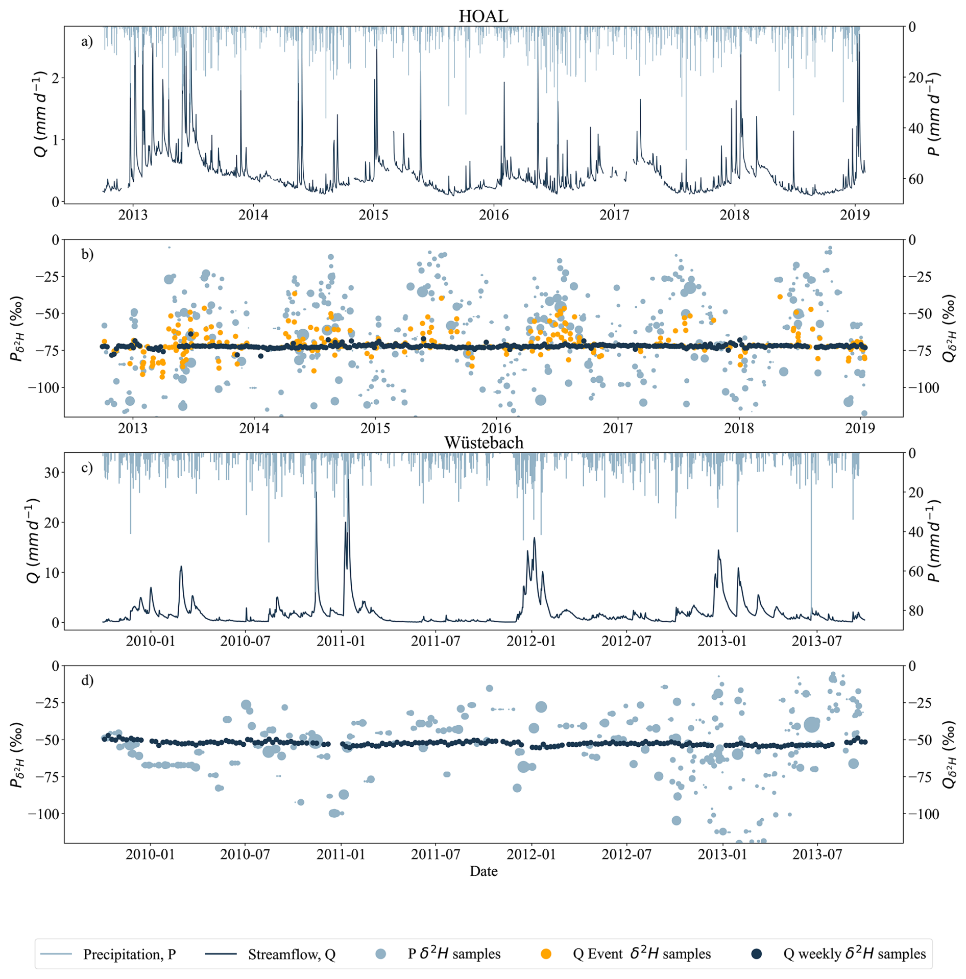
Figure 1 Hydrological and tracer data of the HOAL and Wüstebach catchments. (a, c) daily measured streamflow Q (mm d⁻¹) and precipitation P (mm d⁻¹), (b, d) precipitation δ²H signals (light blue) and streamflow δ²H signals (dark blue); the size of the dots indicates the relative precipitation volume. For the HOAL catchment, the δ²H data of streamflow were further shown as the weekly grab samples (b, dark blue dots) and event samples (b, orange dots). For the HOAL catchment, precipitation δ²H samples are in daily resolution, whereas for the Wüstebach catchment, beginning in September 2012, the sampling frequency for precipitation δ²H increased from weekly to daily (d).

In the Wüstebach catchment, precipitation data were obtained from a nearby meteorological station operated by the German Weather Service (Deutscher Wetterdienst, DWD station 3339), and stream discharge was measured using a V-notch weir for low flows and a Parshall flume for high flows (Bogena et al., 2015). The precipitation samples for isotopic analysis were collected at the Schöneseiffen meteorological station, located approximately 3 km northeast of the catchment at an elevation of 620 m a.s.l. Starting in June 2009, weekly precipitation samples were collected using a cooled storage rain gauge with 2.3 L HDPE bottles (Stockinger et al., 2014). From September 2012 onward, the sampling resolution was increased to daily intervals (Fig. 1d) using a cooled automated sampler (Eigenbrodt GmbH & Co. KG, Germany; 250 mL PE bottles). Stream water samples for isotopic analysis were collected weekly at the catchment outlet as grab samples. Cavity ring-down spectroscopy (Picarro L2120-i, L2130-i) was used for water isotope analyses, with an analytical uncertainty of ±0.1 ‰ for δ¹⁸O and ±1.0 ‰ for δ²H. All isotopic measurements are reported as per mil (‰) relative to Vienna Standard Mean Ocean Water (VSMOW).

2.3 Tracer transport model

We used a process-based tracer transport model (Türk et al., 2025) based on the previously developed dynamic mixing tank (DYNAMITE) modelling framework (Hrachowitz et al., 2014), which allows for the simultaneous representation of water fluxes and tracer transport (Hrachowitz et al., 2013) and includes the concept of storage-age selection functions (Rinaldo et al., 2015). Briefly, both the HOAL and Wüstebach catchments are conceptualised through five interconnected reservoirs: snow, canopy interception, unsaturated root zone, fast responding storage (shallow soil water), and groundwater with active and passive components (Fig. 2). The model hydrological fluxes are: total precipitation P (mm d⁻¹), precipitation as snow P_s (mm d⁻¹), precipitation as rain P_r (mm d⁻¹), snow-melt P_m (mm d⁻¹), throughfall P_e (mm d⁻¹), interception evaporation E_i (mm d⁻¹), evaporation from the root zone E_a (mm d⁻¹), preferential fast response R_f (mm d⁻¹), fast preferential recharge to the to groundwater R_fs (mm d⁻¹, preferential fast response R_ff (mm d⁻¹), infiltration-excess overland flow Q_o (mm d⁻¹), preferential fast response to the fast-responding bucket R_fn (mm d⁻¹), flow from the fast-responding reservoir Q_f (mm d⁻¹), saturation-excess overland flow from the fast-response bucket Q_of (mm d⁻¹), slow recharge to the groundwater reservoir R_s (mm d⁻¹), baseflow from the groundwater reservoir Q_s (mm d⁻¹), deep infiltration loss Q_l (mm d⁻¹), and the total discharge to the streamflow Q_tot (mm d⁻¹). Model calibration parameters are shown in red adjacent to the model component they are associated with (Fig. 2), and symbols are defined in Table S2 in the Supplement. All model equations are defined in Table S1.

To trace δ²H fluxes through the model, the SAS approach (Rinaldo et al., 2015; Harman, 2015) was integrated into the hydrological model. In this integrated framework, each storage defined within the hydrological model (e.g., S_r,S_f, Fig. 2), at any given time t, stores water of different ages, represented as T, which traces back to past precipitation and is ranked by their input time. The age distribution of a storage at time t is termed p_s(T,t), and is in its cumulative form S_T(T,t), also known as the cumulative residence time distribution (RTD). The output fluxes O (mm d⁻¹) (e.g., E_a,R_s, Fig. 2) are subsets of specific ages from the storage with water age distributions termed $p_{Q,T}(T,t)$, which are known in their respective cumulative form O_T(T,t) as cumulative transit time distributions (TTD). The relation between storage and output fluxes is formulated based on the SAS function ${\mathit{\omega }}_{O,m,j}$ that SAS defines as the likelihood of selecting water parcels of different ages for release from the storage, thereby translating the internal age structure of the storage into an age distribution of output fluxes. At each time t, the age-ranked water in storage is characterized by its tracer composition C_S(T,t), which reflects the signal of past precipitation inputs. The output fluxes are likewise described by their tracer distributions, C_O(T,t), derived from the selection of water ages leaving storage.

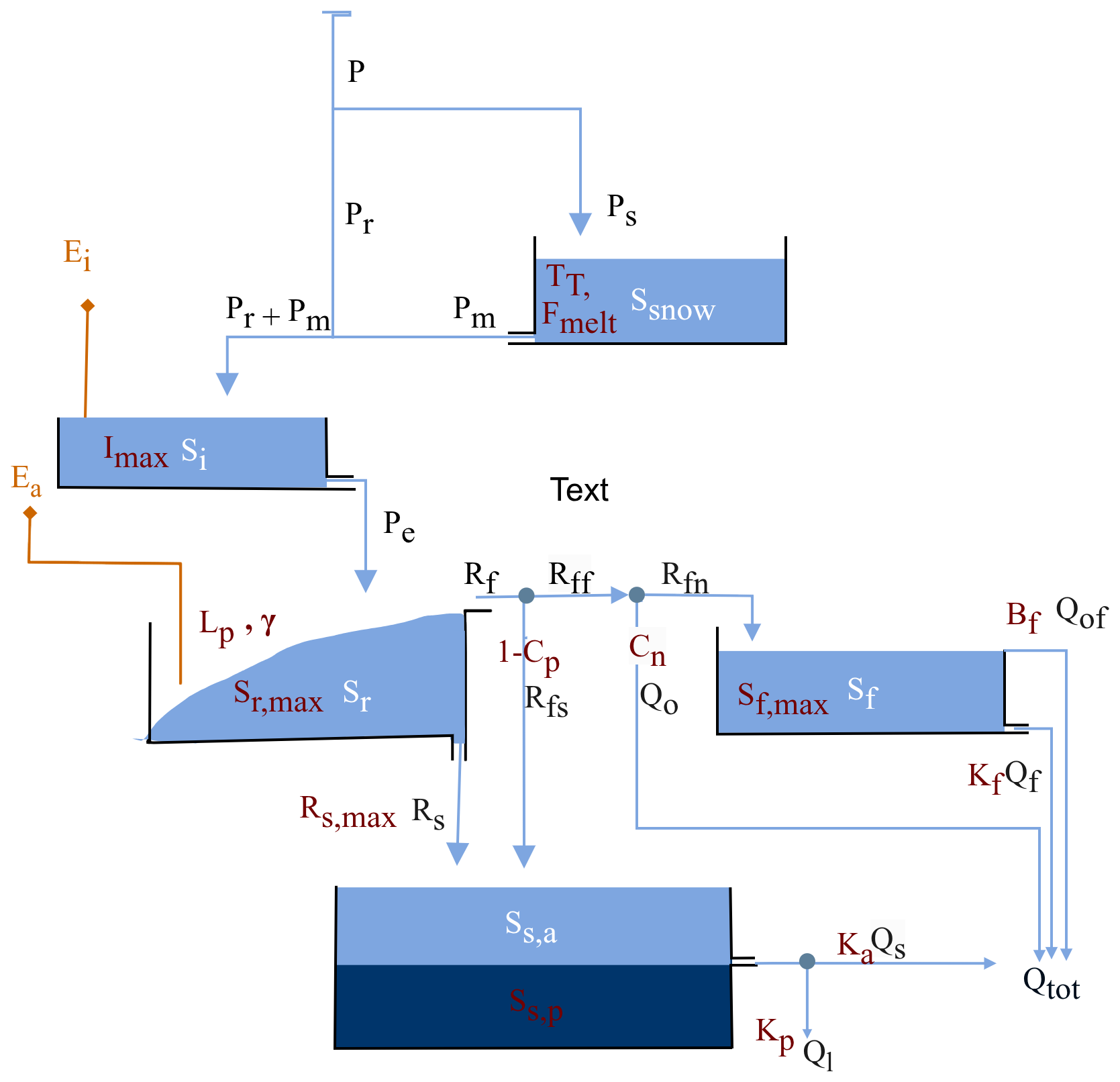
Figure 2 The model structure used to represent the HOAL and the Wüstebach catchment (adapted from Türk et al., 2025). Light blue boxes indicate the hydrologically active storage volumes that contribute to total discharge Q_tot: Snow storage (S_snow), canopy interception (S_i), fast response bucket (S_f), root zone storage (S_r), and “active” groundwater (S_s,a). The darker blue box (S_s,p) indicates a hydrologically “passive” groundwater volume. Blue lines indicate snow and water fluxes which are total precipitation P (mm d⁻¹), precipitation as snow P_s (mm d⁻¹), precipitation as rain P_r (mm d⁻¹), snow-melt P_m (mm d⁻¹), throughfall P_e (mm d⁻¹), preferential fast response R_f (mm d⁻¹), fast preferential recharge to the to groundwater R_fs (mm d⁻¹), preferential fast response R_ff (mm d⁻¹), infiltration-excess overland flow Q_o (mm d⁻¹), preferential fast response to the fast-responding bucket R_fn (mm d⁻¹), flow from the fast-responding reservoir Q_f (mm d⁻¹), saturation-excess overland flow from the fast-response bucket Q_of (mm d⁻¹), slow recharge to the groundwater reservoir R_s (mm d⁻¹), baseflow from the groundwater reservoir Q_s (mm d⁻¹), deep infiltration loss Q_l (mm d⁻¹), and the total discharge to the streamflow Q_tot (mm d⁻¹). Orange lines indicate water vapour fluxes; interception evaporation E_i (mm d⁻¹), evaporation from the root zone E_a (mm d⁻¹). Model parameters are shown in red adjacent to the model component they are associated with, and symbols are defined in Table S2. All model equations are defined in Table S1.

Then, the transport balance of the storage is built on water age conservation over time:

$$\begin{array}{}\text{(1)}& \begin{array}{rl}{\displaystyle \frac{\partial S_{T,j}(T,t)}{\partial t}}& +{\displaystyle \frac{\partial S_{T,j}(T,t)}{\partial T}}=\sum _{n=\mathrm{1}}^N{I}_{T,n,j}(T,t)\\ & -\sum _{m=\mathrm{1}}^M{O}_{T,m,j}(T,t)\end{array}\end{array}$$

where: $\frac{\partial S_{\mathrm{T}}(T,t)}{\partial t}$ is the rate of change of age-ranked storage with respect to time, $\frac{\partial S_{\mathrm{T}}(T,t)}{\partial T}$ represents the ageing of water within the storage (e.g., S_r,S_f) , $I_{T,n}(T,t)$ are the cumulative age-ranked inflows $O_{T,m,j}(T,t)$ are the cumulative age-ranked outflows. N and M denote the number of inflows and outflows from a given storage component (e.g., for the root zone, N would be P_e, and M is E_a, R_f, and R_s; see Fig. 2). Each age-ranked outflow $O_{T,m,j}(T,t)$ (Eq. 2) from a specific storage component j depends on the cumulative age distribution of that outflow $P_{O,m,j}(T,t)$ and outflow volume O_m,j(t), which is estimated by the hydrological balance component of the model.

$$\begin{array}{}\text{(2)}& O_{T,m,j}(T,t)=O_{m,j}\left(t\right)P_{O,m,j}(T,t),\end{array}$$

where O_m,j(t) is the total outflow rate, and

$$\begin{array}{}\text{(3)}& P_{O,m,j}(T,t)={\mathrm{\Omega }}_{o,m,j}\left(S_{T,j}\right(T,t),t)\end{array}$$

The cumulative age distribution $P_{O,m,j}(T,t)$ (Eq. 3) is the backward TTD of that outflow in cumulative form and depends on the age-ranked distribution of water in the storage component j at time t, $S_{T,j}(T,t)$, and the probability density function, which in this case is the SAS function ${\mathit{\omega }}_{O,m,j}$ (or O_T(T,t) in its cumulative form) of that flux.

From the cumulative age distribution, the associated probability density function can be derived according to

$$\begin{array}{}\text{(4)}& p_{o,m,j}(T,t)={\stackrel{\mathrm{‾}}{\mathit{\omega }}}_{o,m,j}\left(S_{T,j}\right(T,t),t){\displaystyle \frac{\partial S_{T,j}(T,t)}{\partial T}},\end{array}$$

where ${\mathit{\omega }}_{o,m,j}(S,t)$ is a probability density function of normalized rank storage $S_{T,\mathrm{norm},j}(T,t)$ (Eq. 5). Normalizing the age-ranked storage S_T(T,t) by its total volume S_j(t) constrains $S_{T,\mathrm{norm},j}$ to the interval [0,1] and holds mass balance without requiring rescaling of the SAS function at each time step.

$$\begin{array}{}\text{(5)}& S_{T,\mathrm{norm},j}(T,t)={\displaystyle \frac{S_{T,j}(T,t)}{S_j\left(t\right)}},\end{array}$$

so that $\mathrm{0}\le S_{T,\mathrm{norm},j}\le \mathrm{1}$.

Finally, the tracer composition of outflow m from compartment j is computed as:

$$\begin{array}{}\text{(6)}& C_{O,m,j}\left(t\right)=\underset{\mathrm{0}}{\overset{S_j}{\int }}{C}_{S,j}\left(S_{T,j}\right(T,t),t){\stackrel{\mathrm{‾}}{\mathit{\omega }}}_{O,m,j}\left(S_{T,j}\right(T,t),t)\mathrm{d}{S}_T\end{array}$$

where $C_{O,m,j}\left(t\right)$ is the tracer composition in outflow m from storage component j at time t, and C_S,j is the tracer composition in storage at time t. The model reproduces TTDs for all fluxes and storage components (Fig. 2) at each time step t. Further details on the model architecture and assumptions can be found in previous studies (Hrachowitz et al., 2014; Fovet et al., 2015). The water balance and flux equations for the two catchments in this study application are described in Türk et al. (2025) and provided in Table S1.

Similar to previous tracer transport studies for the HOAL (Türk et al., 2025) and Wüstebach (Hrachowitz et al., 2021) catchments, we used beta distributions to formulate the SAS functions. Beta distributions are defined by two shape parameters (α and β). When both parameters of the Beta distribution were equal to 1 ($\mathit{\alpha }=\mathit{\beta }=\mathrm{1}$), water is uniformly sampled from storage without any preference for specific ages. If α<β (or α>β), a selection preference for younger (or older) water existed, respectively. In this study, α was varied during calibration to represent different degrees of preferential selection of younger or older water, while β was fixed at 1 to reduce parameter dimensionality and avoid over-parametrization. Fixing β=1 follows previous applications of SAS functions (van der Velde et al., 2015; Hrachowitz et al., 2021) and provides a parsimonious way to explore age-selection behaviour by varying a single shape parameter, while still allowing deviations from uniform mixing. The time variability of the SAS function shape was then determined by the age-ranked storage and the shape parameter α, which was bounded between 0 and 1 to represent a preference for younger storage, and greater than 1 to represent a preference for older storage. Preferential release of older water (α>1) decreases the mean residence time of stored water, as older water is removed from storage. Conversely, preferential release of younger water (α<1) increases the mean residence time of stored water, as older water remains stored for longer periods.

In principle, the model has 16 hydrological fluxes (Fig. 2), and each of the fluxes (e.g., E_a,R_s) requires a separate SAS function parameter α to be calibrated. However, this is computationally infeasible and would introduce additional model parameter interactions. Therefore, for all modelled hydrological fluxes, α and β were fixed at 1, except those representing preferential flow from the unsaturated root zone (named as S_U,alpha Table S2) for model calibration.

In the Wüstebach catchment, previous studies (Wiekenkamp et al., 2016; Hrachowitz et al., 2021) showed that catchment soil wetness is the main driver for activating preferential flow pathways in the unsaturated zone, leading to the preferential release of younger water to the streamflow as soil wetness increases. Therefore, the SAS function shape parameter representing preferential flow from the unsaturated root zone (R_f, Fig. 2) was formulated as a time-variable function of relative soil wetness ($S_{\mathrm{r}}/S_{\mathrm{r},\max }$), where S_r is the water volume in the root zone at time t, and S_r,max is the maximum root-zone storage capacity (calibrated parameter). Equation (8) adopts an increasing probability of younger water release with increasing soil wetness through the time-dependent shape parameter α(t), reflecting changes in transport processes between wet and dry soil conditions.

In the HOAL catchment, previous studies have highlighted the non-linearity of preferential flow generation in the unsaturated zone, where both precipitation intensity and soil wetness control the activation of preferential flow pathways (Széles et al., 2020; Vreugdenhil et al., 2022). In addition to saturation excess overland flow (when $\frac{S_{\mathrm{r}}\left(t\right)}{S_{\mathrm{r},\max }}>\mathrm{1}$), infiltration excess overland flow also occurs when precipitation intensity exceeds a certain threshold, routing recent precipitation directly to the stream with minimal interaction with stored water (Türk et al., 2025). To account for the combined roles of soil wetness and precipitation intensity in the activation of preferential flow and the release of younger water in HOAL catchment, we parameterized the SAS function for preferential flow from the unsaturated root zone (R_f, Fig. 2) using a time-variable shape parameter α(t) defined as a function of both soil wetness state and precipitation intensity. Specifically, α(t) was formulated as a function of relative soil wetness (scaled by the maximum root-zone storage capacity, S_r,max) and precipitation intensity (P_I, mm d⁻¹), with a threshold parameter (P_thresh) controlling the onset of precipitation-driven preferential flow. This causal formulation was implemented to ensure that α(t) dynamically responds to both wetness conditions and event-scale precipitation forcing, allowing the model to capture the non-linear activation of preferential flow observed in the catchment. The dual dependence of α(t) on soil wetness and precipitation intensity, therefore, extends previous SAS applications by providing a more flexible representation of unsaturated zone preferential flow dynamics in HOAL.

For the HOAL catchment, the time variability of α for preferential flow in the unsaturated root zone was defined as:

$$\begin{array}{}\text{(7)}& \mathit{\alpha }\left(t\right)=\left\{\begin{array}{ll}{\mathit{\alpha }}_{\mathrm{0}},& \text{if }{P}_{\mathrm{r}}\left(t\right)\ge P_{\mathrm{thresh}}\\ \mathrm{1}-\frac{S_{\mathrm{r}}\left(t\right)}{S_{\mathrm{r},\max }}(\mathrm{1}-{\mathit{\alpha }}_{\mathrm{0}}),& \text{if }{P}_{\mathrm{r}}\left(t\right)<P_{\mathrm{thresh}}\end{array}\right.\end{array}$$

For the Wüstebach catchment, time variability of α for the preferential flow in the unsaturated root zone was defined as:

$$\begin{array}{}\text{(8)}& \mathit{\alpha }\left(t\right)=\mathrm{1}-\left({\displaystyle \frac{S_{\mathrm{r}}\left(t\right)}{S_{\text{r,max}}}}\right)(\mathrm{1}-{\mathit{\alpha }}_{\mathrm{0}})\end{array}$$

In both Eqs. (7) and (8), the time variable shape parameter α(t) controls the preferential release of younger water: values of $\mathrm{0}<\mathit{\alpha }\left(t\right)<\mathrm{1}$ indicate a bias towards younger water parcels, whereas α(t)=1 corresponds to uniform sampling. The α₀ is a calibration parameter representing the lower bound between 0 and 1, allowing α(t) to vary between α₀ and 1. When soil wetness is low (S_r(t)≪S_r,max), α(t) approaches 1, indicating uniform sampling. As soil wetness increases (S_r(t) approaches S_r,max), α(t) decreases towards α₀, reflecting a stronger preference for younger water. In Eq. (7), the lower bound α₀ is applied directly whenever precipitation intensity exceeds a certain threshold (P_thresh).

2.3.1 Model calibration and evaluation

We calibrated the model simultaneously against both streamflow and stable water isotopes to ensure that both hydrological and tracer information were integrated during parameter optimisation. We used daily time steps in the model parameter calibration for the period from October 2014 to 2019 for the HOAL catchment and for the period from October 2010 to October 2013 for the Wüstebach catchment to model streamflow Q (mm d⁻¹) and δ²H signature. The model spin-up period was one year for both catchments; i.e., from October 2013 to October 2014 for the HOAL catchment, and from October 2009 to October 2010 for the Wüstebach catchment.

For model parameter optimization, we used the Differential Evolution algorithm (Storn and Price, 1997) and an objective function that combined five performance criteria related to streamflow and δ²H dynamics. The objective function included the Nash-Sutcliffe efficiencies (NSE) of streamflow (to evaluate overall discharge dynamics), logarithmic streamflow (to match low-flow conditions), the flow duration curve (to capture the distribution of flows over time), the runoff coefficient averaged over three months (to ensure water balance consistency), and the NSE of the δ²H signal in streamflow (to constrain δ²H dynamics) (Table S3). These individual performance metrics were aggregated into the Euclidean distance D_E, with equal weights assigned to streamflow and the δ²H signature, according to:

$$\begin{array}{}\text{(9)}& D_{\mathrm{E}}=\sqrt{{\displaystyle \frac{\mathrm{1}}{\mathrm{2}}}({\displaystyle \frac{{\sum }_{i=m}^M(\mathrm{1}-E_{Q,m}{)}^{\mathrm{2}}}{M}}+{\displaystyle \frac{{\sum }_{i=n}^N(\mathrm{1}-E_{\mathrm{18}O,n}{)}^{\mathrm{2}}}{N}})}\end{array}$$

where M=4 is the number of performance metrics with respect to streamflow, N=1 is the number of performance metrics for tracers, and E is the evaluation matrix based on goodness-of-fit criteria. The Euclidean distance D_E to the “optimal model” (where D_E=0 indicates a perfect fit) was used to ensure that overall model performance remained balanced. Only solutions achieving D_E≤1 were accepted as feasible solutions for further analysis. The accepted solutions were then ranked in order of decreasing D_E, and the solution with the lowest D_E was selected as the parameter set for TTD estimations. Transit times were estimated up to a tracking period of 1000 d, limited by data availability, and the mean of the estimated TTD was compared between dry periods (streamflow below the 25th percentile, Q₂₅) and wet periods (streamflow above the 75th percentile, Q₇₅). In addition, the young-water fraction of daily streamflow (F_Q(T<90)) was calculated as the sum of streamflow fractions with transit times up to 90 d. Its monthly variability was then analyzed in relation to the corresponding monthly variability of soil wetness $\left(\frac{S_{\mathrm{r}}}{S_{\mathrm{r},\max }}\right)$ for both catchments.

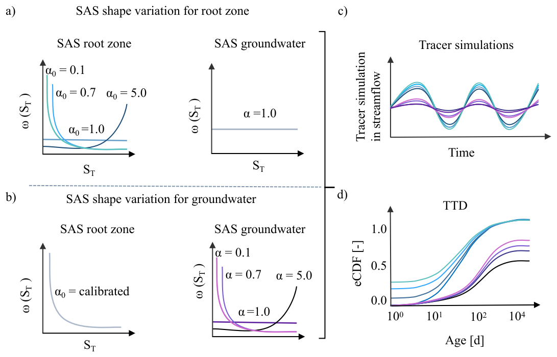
Figure 3 Conceptual representation of the sensitivity analysis illustrating how different SAS functions, formulated with the lower bound of the shape parameter α₀ for root-zone preferential flow and α for groundwater flow, affect the modelled tracer signals and inferred transit time distributions (TTDs). (a) The unsaturated root-zone SAS function shape parameter α₀ is varied from 0.1 (strong young-water preference, light blue line) to 5.0 (old-water preference, dark blue line), while the groundwater age selection remains uniform. (b) The root-zone SAS function shape parameter α₀ is fixed at its calibrated value, and the groundwater α is varied from 0.1 (strong young-water preference, light purple line) to 5.0 (old-water preference, dark purple line). (a, b) The x-axis, S_T, represents the age-ranked storage, and the y-axis, ω(S_T), denotes the relative probability of releasing water of that age. (c, d) Illustrate the modelled tracer time series based on the scenarios implemented in (a) and (b), and the corresponding empirical cumulative transit time distributions.

2.3.2 Sensitivity test of root zone and groundwater SAS functions

In this analysis, we systematically tested the sensitivity of the streamflow δ²H signal simulations and inferred transit times to changes in the StorAge Selection (SAS) function parameterization for both the unsaturated root zone and the groundwater compartments. We first tested the sensitivity of the streamflow δ²H signal to root-zone preferential flow by systematically varying the lower bound of the SAS shape parameter α₀ across four values: 0.1 (very young-water preference), 0.7 (young-water preference), 1.0 (uniform selection), and 5.0 (older-water preference), while keeping the groundwater SAS function uniform (i.e., α=1; Fig. 3a). This approach assesses whether different parametrizations of the SAS function for root-zone preferential pathways alone could reveal a strong impact on the modelled streamflow δ²H time series and the inferred transit times. Next, we tested the sensitivity of the δ²H signal to changes in the groundwater SAS function (Fig. 3b) by varying α across the same range – 0.1, 0.7, 1.0, and 5.0 – by using the previously calibrated optimized α₀ value for the root-zone preferential flow. Here, α (rather than α₀) is used because, in the groundwater (saturated) zone, relative wetness is assumed to be constant and equal to one; consequently, the SAS shape parameter is not time-variable. This second test was designed to show if (and how) different parametrizations of the SAS function for groundwater flow influence the modelled streamflow δ²H and time series transit time distributions. We evaluated the model’s performance in simulating δ²H using Spearman rank correlation, NSE${}_{{\mathit{\delta }}^{\mathrm{2}}\mathrm{H}}$, and MAE${}_{{\mathit{\delta }}^{\mathrm{2}}\mathrm{H}}$. Finally, we calculated daily cumulative TTDs and compared how their means changed across all scenarios to quantify the impact of SAS function shape on modelled water age distributions. The SAS formulation can only indicate whether preferential release of younger water occurs. It does not capture the physical processes driving this behavior, such as soil hydraulic properties, macropore flow, or transient groundwater connectivity.

To isolate the effect of the SAS function shape on the modelled streamflow δ²H signal and on the estimated transit time distributions (TTDs), all hydrological model parameters (e.g., maximum percolation rate, storage capacities, and flow path configurations) were kept identical to the individually calibrated values for the HOAL and Wüstebach catchments. By using the same calibrated parameters while testing different SAS parameterizations for HOAL and Wüstebach, any differences in the modelled δ²H signals or TTDs can therefore be attributed solely to changes in the SAS function parameterization.

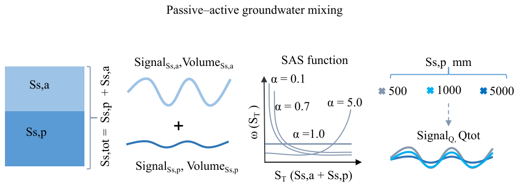
Figure 4 Conceptual representation of the sensitivity analysis illustrating how different passive storage volumes ($S_{\mathrm{s},\mathrm{p}}=\mathrm{500}$, 1000, and 5000 mm) interact with the active storage volume (S_s,a) under various groundwater SAS function shapes affecting tracer simulations in streamflow. The groundwater SAS function parameter α is varied from 0.1 (strong young-water preference) to 5.0 (old-water preference). For the SAS function, the x-axis, S_T, represents the age-ranked total groundwater storage, and the y-axis, ω(S_T), denotes the relative probability of releasing water of that age.

2.4 Passive groundwater storage volumes and mixing assumptions with the active groundwater storage

In this analysis, we tested whether and to what extent the mixing of the passive groundwater storage with the active groundwater modulates the δ²H signal in streamflow and, consequently, influences model performance and inferred transit times. We extended the stepwise analysis (Fig. 3b) by varying passive storage volumes (Fig. 4). In the model setup, groundwater storage was represented as an active component (S_s,a) and a hydrologically passive component (S_s,p, mm). The passive groundwater storage (S_s,p) does not contribute to the quantity of baseflow; it exchanges older water with the active groundwater storage (S_s,a), thereby influencing the age composition and isotopic signature of the baseflow (Q_s, Fig. 2) that contributes to streamflow. For the SAS formulation, total groundwater storage was defined as the sum of active and passive components ($S_{\mathrm{s},\mathrm{tot}}=S_{\mathrm{s},\mathrm{a}}+S_{\mathrm{s},\mathrm{p}}$), such that the age-ranked total storage (S_s,tot) represents the combined influence of active and passive storage on the age composition of baseflow and thereby on the age composition streamflow (Fig. 4)

We applied three different passive storage volumes ($S_{\mathrm{s},\mathrm{p}}=\mathrm{500}$, 1000, and 5000 mm) based on the values reported for comparable headwater catchments (Birkel et al., 2011; Benettin et al., 2015a; Hrachowitz et al., 2021). To isolate the effect of passive storage and age-selection parameterization on streamflow δ²H dynamics and TTD estimations, we kept all hydrological model parameters (e.g., maximum percolation rate, storage capacities, and flow path configurations) identical to the individually calibrated values for the HOAL and Wüstebach catchments. Similar to Fig. 3b, four different groundwater SAS parameterizations were tested (Fig. 4): a strong preference for younger water (α=0.1), a preference for younger water (α=0.7), uniform selection (α=1.0), and a preference for older water (α=5.0). We evaluated model performance in simulating streamflow δ²H by comparing measured and modelled isotope signals using ${\mathrm{NSE}}_{{\mathit{\delta }}^{\mathrm{2}}\mathrm{H}}$ and ${\mathrm{MAE}}_{{\mathit{\delta }}^{\mathrm{2}}\mathrm{H}}$. In addition, we calculated daily cumulative TTDs and compared the means of these distributions across different passive storage volumes and SAS parametrizations.

3 Results

3.1 Variation of δ²H in precipitation and streamflow

In the HOAL catchment, δ²H values in precipitation ranged from −3.0 ‰ to −150.0 ‰ (Fig. 1b), with a volume-weighted mean of $-\mathrm{67.7}\mathrm{‰}\pm \mathrm{31.9}\mathrm{‰}$. Event-based streamflow δ²H samples ranged from −26.2 ‰ to −108.0 ‰ (Fig. 1b), while weekly streamflow δ²H samples ranged from −73.2 ‰ to −75.2 ‰. The overall volume-weighted mean of stream samples was $-\mathrm{71.6}\mathrm{‰}\pm \mathrm{6.1}\mathrm{‰}$.

In the Wüstebach catchment, δ²H values in precipitation ranged from −4.3 ‰ to −163.2 ‰ (Fig. 1d, light blue dots), with a volume-weighted mean of $-\mathrm{52.2}\mathrm{‰}\pm \mathrm{21.4}\mathrm{‰}$. Weekly streamflow δ²H values exhibited smaller variations, ranging from −45.6 ‰ to −57.1 ‰ (Fig. 1d). The volume-weighted mean of stream samples was $-\mathrm{53.2}\mathrm{‰}\pm \mathrm{1.4}\mathrm{‰}$.

Overall, δ²H in precipitation exhibited large variability in both catchments; however, this signal was attenuated in streamflow. In the HOAL catchment, event-based streamflow δ²H samples reflected how precipitation inputs were rapidly transmitted to the stream, whereas weekly samples alone would have masked this variability. This highlights the importance of event-based sampling for detecting preferential flow signals, which may remain obscured with weekly data alone. This applies to the Wüstebach catchment, where only weekly streamflow δ²H measurements were available, which may have prevented the detection of such rapid responses.

3.2 Model calibration

Model calibration resulted in 55 feasible (acceptable model performance with DE <1) parameter solutions for HOAL (Fig. S3) and 190 feasible parameter solutions for the Wüstebach catchment (Fig. S4). The model reproduced the main features (e.g the rise and recession limbs) of the hydrograph and captured both the timing and magnitude of high and low flow events for the simulation period from October 2014 to 2019 for HOAL (Fig. S5a, d) and from October 2010 to October 2013 for the Wüstebach catchment (Fig. S5e, h).

For the HOAL catchment, the mean Nash-Sutcliffe efficiency of streamflow (NSE_Q) for the 55 solutions was 0.60 (Fig. S6). Minor dissimilarities occurred during the spring of 2016, when low flows were overestimated (Fig. S5a). Nevertheless, the model modelled most other observed flow signatures reasonably well (Fig. S6). Among the 55 solutions, the mean NSE for low flows (NSE_log Q) was 0.65, for the flow duration curve (NSE_FDC) was 0.53, and for the three-month averaged runoff ratio (NSE_RC) it was 0.85. For several rain events, the model captured δ²H fluctuations during high flows and maintained a stable δ²H signal during low flows, with a mean ${\text{NSE}}_{{\mathit{\delta }}^{\mathrm{2}}\text{H}}$ of 0.51. Overall, the Euclidean distance (D_E) for these 55 solutions ranged from 0.60 to 0.33 (Fig. S6).

For the Wüstebach catchment, the mean NSE of streamflow (NSE_Q) for the 190 solutions was 0.78 (Fig. S6). Minor dissimilarities occurred during the spring of 2012, when low flows were overestimated, and the winter of 2012, when peak flows were underestimated (Fig. S5e). Among the 190 solutions, the mean NSE for low flows (NSE_log Q) was 0.65, for the flow duration curve (NSE_FDC) it was 0.93, and for the three-month averaged runoff ratio (NSE_RC) it was 0.91. For several rain events, the model captured δ²H fluctuations during high flows and maintained a stable δ²H signal during low flows, with a mean ${\text{NSE}}_{{\mathit{\delta }}^{\mathrm{2}}\text{H}}$ of 0.58. Overall, the Euclidean distance (D_E) for these 190 solutions ranged from 0.62 to 0.32 (Fig. S6).

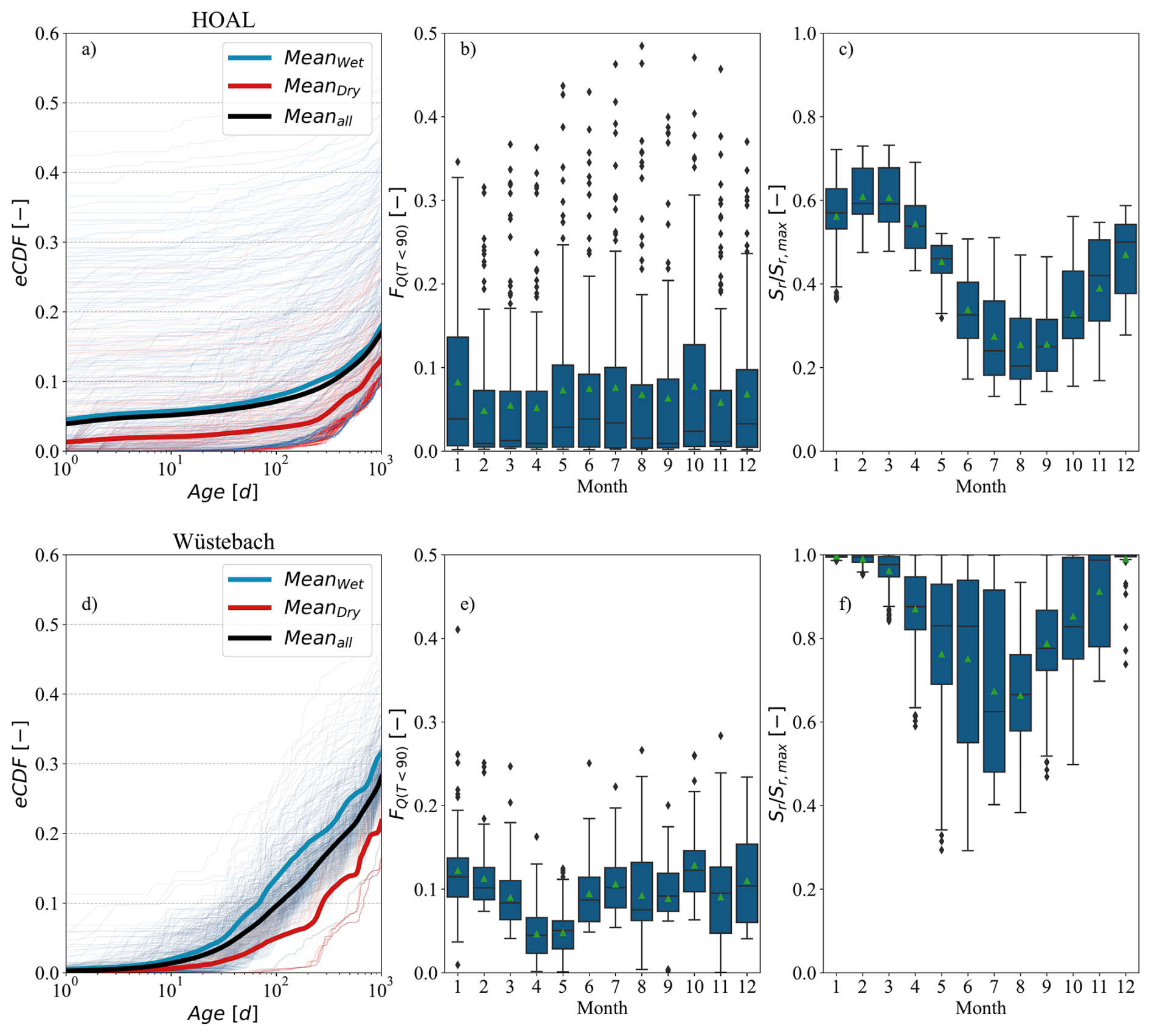
Figure 5 Modelled empirical cumulative transit time distributions (TTDs) for daily streamflow in the (a) HOAL and (d) Wüstebach catchments. The colour of the lines corresponds to the wetness state, where dark blue indicates a wet period and dark red indicates a dry period. In panels (a) and (d), the mean of the empirical cumulative TTDs is shown for the entire tracking period (black line), the dry period (red line), and the wet period (dark blue line). The fraction of streamflow younger than 90 d, F_Q(T<90), grouped by month of the year, is shown in panels (b) and (e) for the HOAL and Wüstebach catchments, respectively. modelled relative soil wetness $\left(\frac{S_{\mathrm{r}}}{S_{\mathrm{r},\max }}\right)$, also grouped by month of the year, is shown in panels (c) and (f) for the HOAL and Wüstebach catchments, respectively. Green triangles in panels (b), (c), (e), and (f) show the mean values.

3.3 Modelled catchment transit times

Figure 5 presents the transit time distributions (TTDs) estimated from the initial model calibration, conducted before the sensitivity analysis. For TTD estimations, we used the model-calibrated parameter set that yielded the lowest D_E. The results presented hereafter are conditional on the underlying model assumptions and should be interpreted in light of the associated uncertainties. In the HOAL catchment, the fraction of streamflow younger than 1000 d exhibited considerable variability, ranging from 5 % to 50 % (Fig. 5a). The mean fraction of discharge younger than 1000 d was 13 %; it increased to 15 % during wet periods and decreased to 10 % during dry periods (Fig. 5a). The value of the fraction of streamflow younger than 90 d, F_Q(T<90 d), varied widely within the same calendar month, ranging from 2 % to 45 %; however, the mean F_Q(T<90 d) across months did not exhibit pronounced seasonal patterns (Fig. 5b). The mean value of modelled relative soil saturation ($S_{\mathrm{r}}/S_{\mathrm{r},\max }$) varied from 0.25 to 0.60 (Fig. 5c).

In the Wüstebach catchment, the mean fraction of discharge younger than 1000 d was 27 %, increasing to 35 % during wet periods and decreasing to 20 % during dry periods (Fig. 5d). The value of the fraction of streamflow younger than 90 d, F_Q(T<90 d) within the same calendar month ranged between 5 % and 30 % (Fig. 5e), with mean values exhibiting seasonal patterns. The monthly mean of modelled relative soil saturation ($S_{\mathrm{r}}/S_{\mathrm{r},\max }$) ranged from approximately 0.60 to 0.98 (Fig. 5f).

3.4 Sensitivity of δ²H simulations and TTD estimation to different SAS functions in the root zone

In the HOAL catchment, the calibrated lower limit of the SAS shape parameter (α₀=0.14) for the root-zone indicated a strong preference for very younger water through unsaturated root-zone preferential flow pathways. These reflected the SAS formulation (Eq. 7) on the dual dependence of α(t) on soil wetness and precipitation intensity. Under high-intensity precipitation, α(t) takes a value of 0.14, indicating that rapid activation of preferential pathways occurs, allowing precipitation inputs to reach the stream with minimal mixing with stored water. In contrast, under wetter antecedent conditions, α(t) increases toward 1, indicating greater mixing within the root zone and contributions of relatively older (i.e., older than recent precipitation inputs) water to streamflow.

In the Wüstebach catchment, the calibrated t lower limit of the SAS shape parameter (α₀=0.98) for root-zone suggested only a slight preference for younger water. Here, α(t) varied between 0.98 and 1 depending on the soil wetness state (Eq. 8). Under wetter antecedent conditions, established preferential flow pathways facilitated more mixing compared to overland flow, leading to relatively older (i.e., older than recent precipitation) water contributions.

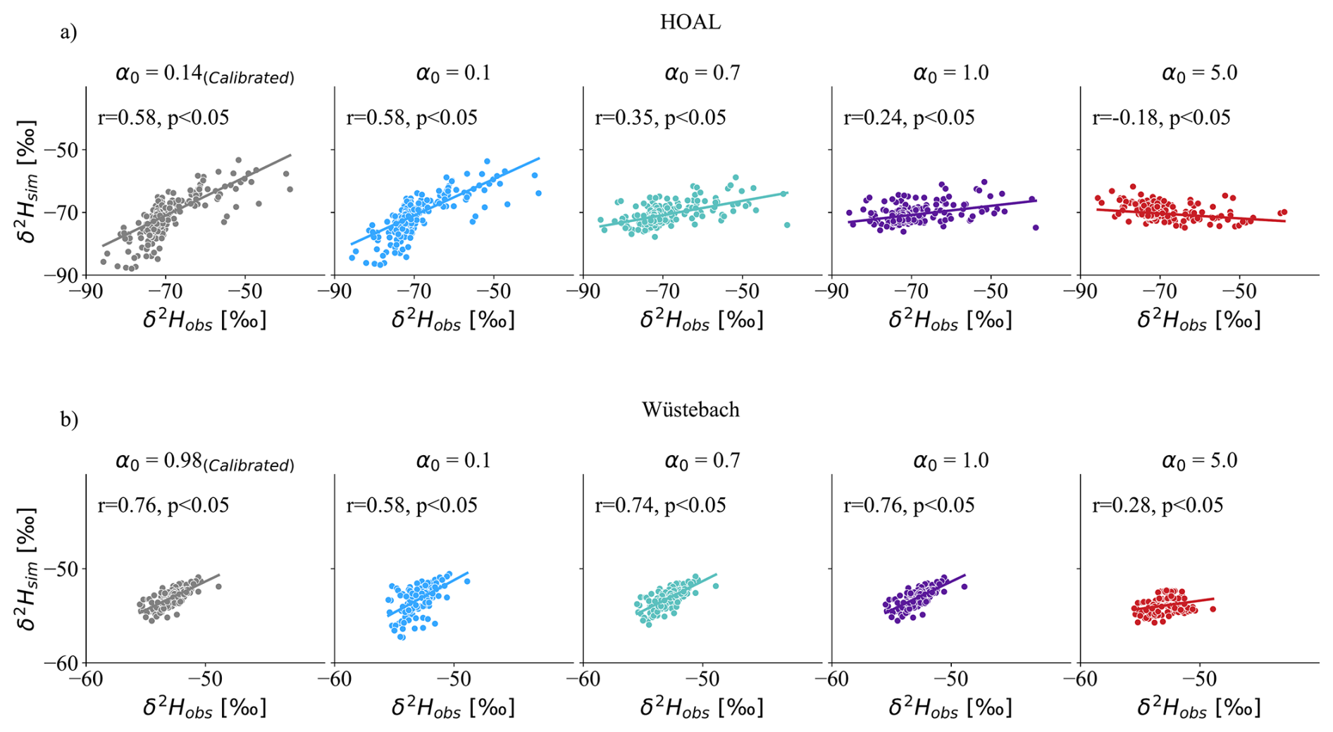
Figure 6 Spearman rank correlations between modelled (y-axis) and observed (x-axis) δ²H signals in streamflow based on varying the SAS shape parameter α₀ [–] in the root zone for (a) HOAL and (b) Wüstebach. The simulations range from very young preference (${\mathit{\alpha }}_{\mathrm{0}}=\mathrm{0}.$1) to old water preference (α₀=5) for the unsaturated root zone preferential flow, while the groundwater flow was uniformly sampled (α=1).

For both catchments, root-zone preferential flow SAS functions ranging from a strong young water preference (α₀=0.1) to uniform sampling (α₀=1.0) produced high (positive) Spearman rank correlations (r) between modelled and observed δ²H. In contrast, an old-water preference (α₀=5.0) yielded negative or weak correlations, indicating a poor fit to the observed tracer signals. In HOAL, the r values ranged between 0.58, and −0.18 for values of α₀ between 0.1 and 5.0 (Fig. 6a). The corresponding Nash-Sutcliffe efficiencies (NSE${}_{{\mathit{\delta }}^{\mathrm{2}}\mathrm{H}}$) ranged between 0.56, and −0.25 (Table 1). In Wüstebach, the r values for modelled δ²H ranged between 0.58, and 0.28 for values of α₀ between 0.1 and 5.0 (Fig. 6b). The corresponding NSE${}_{{\mathit{\delta }}^{\mathrm{2}}\mathrm{H}}$ ranged beetwe 0.51 and −0.14 (Table 1).

The Spearman rank correlations (r) between observed and modelled δ²H were lower in HOAL compared to Wüstebach, which can be attributed in part to differences in temporal resolution and the variability of isotope sampling. In HOAL, streamflow δ²H was sampled on an event basis, with values ranging from −26.2 ‰ to −108.0 ‰ (Fig. 1b). In contrast, the Wüstebach catchment weekly to biweekly sampling scheme yielded streamflow δ²H values between −45.6 ‰ and −57.1 ‰ (Fig. 1b).

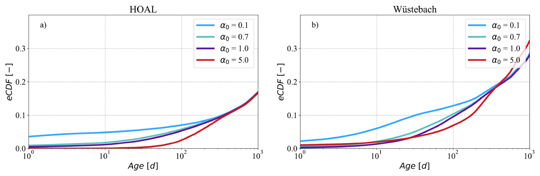
Figure 7 The mean of empirical cumulative distribution functions (eCDFs) of modelled transit times of daily discharge for the (a) HOAL and (b) Wüstebach catchments under varying SAS shape parameters in the unsaturated root zone (${\mathit{\alpha }}_{\mathrm{0}}=\mathrm{0.1},\mathrm{0.7},\mathrm{1.0},\mathrm{5.0}$). (a, b) The simulations range from very young preference (α₀=0.1) to old water preference (α₀=5) for the unsaturated root zone preferential flow, while the groundwater flow was uniformly sampled (α=1).

For both catchments, root-zone preferential flow SAS functions from a preference for younger water (α₀=0.1) to old water (α₀=5.0) influenced the TTD for ages up to 300 d (T<300) (Fig. 7a, b). This is consistent with root-zone storage residence times being predominantly shorter than 300 d (Fig. S8a, c). Consequently, increasing α₀ from 0.1 to 5.0 and thus reducing the relative contribution of younger flows (Fig. 7a, b), shifted the empirical cumulative distribution functions (eCDFs) toward older water within the first 300 d. In the HOAL, the mean fraction of streamflow with T<300 d reached about 10 % (Fig. 7a,) for all root-zone SAS formulations, whereas in Wüstebach, it was about 20 % (Fig. 7b). Overall, these results indicated that root-zone SAS functions with young-water preferences improved the fit to observed streamflow isotopes, highlighting the importance of preferential flow pathways in shaping short transit times and streams δ²H interpretations.

Table 1 Performance metrics for δ²H simulation results under various SAS parameter scenarios for the HOAL and Wüstebach catchments. The table includes the Nash- Sutcliffe efficiency (NSE${}_{{\mathit{\delta }}^{\mathrm{2}}\mathrm{H}}$) and mean absolute error (MAE${}_{{\mathit{\delta }}^{\mathrm{2}}\mathrm{H}}$), and Spearman rank correlation coefficients ($r_{{\mathit{\delta }}^{\mathrm{2}}\mathrm{H}}$) based on SAS shape parameters (α₀) variations in the root zone and groundwater SAS shape parameters (α). Scenarios tested represent preferences for very young water (α=0.1), young water (α=0.7), uniform selection (α=1.0), and old water (α=5.0). For simulations testing SAS function variations in the root zone, the groundwater SAS function was kept uniform. Conversely, when testing groundwater SAS function variations, the root zone compartment was assigned its calibrated shape factor (α₀=0.14 for HOAL and α₀=0.98 for Wüstebach).

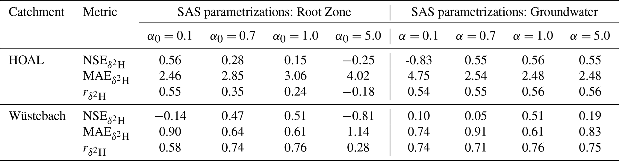
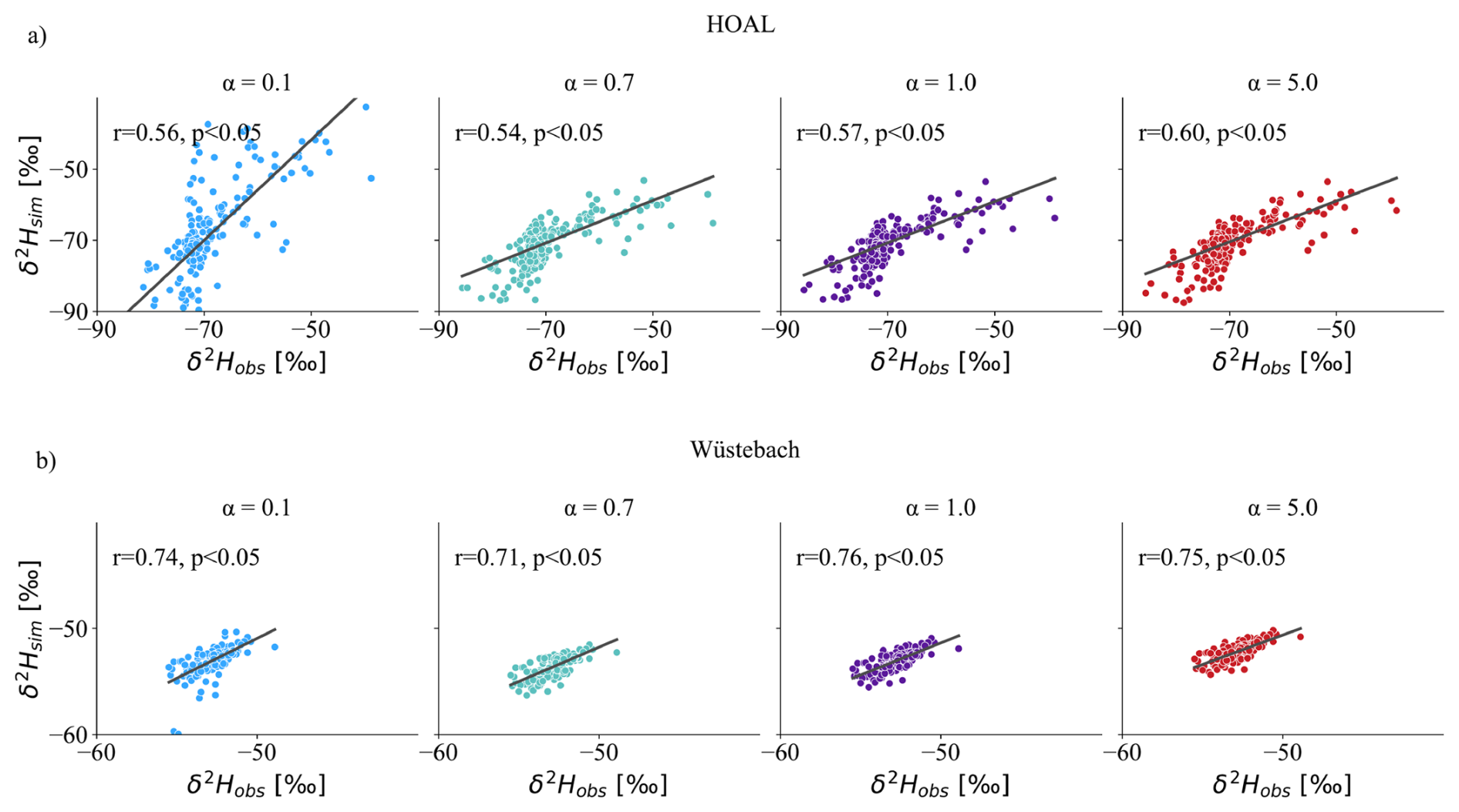
Figure 8 Spearman rank correlations between modelled (y-axis) and observed (x-axis) δ²H signals in streamflow based on varying the SAS shape parameter α [–] in groundwater for (a) HOAL and (b) Wüstebach. The simulations ranged from very young water preference (α=0.1) to old water preference (α=5) for the groundwater, while for the root zone compartment, a calibrated value was used (α₀=0.14 for HOAL and 0.98 for Wüstebach).

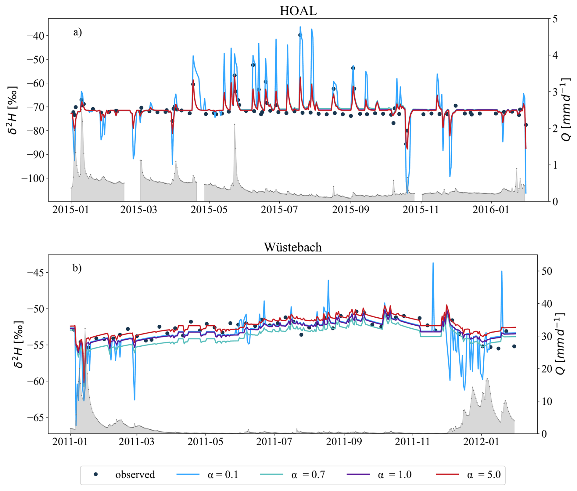
Figure 9 Simulation of δ²H in streamflow based on varying SAS shape parameter α [–] in groundwater for (a) HOAL shown for 2015 and (b) Wüstebach shown for 2011. Simulations over the full tracking period are provided in Fig. S9. The simulations ranged from very young water preference (α=0.1) to old water preference (α=5) for the groundwater, while for the root zone compartment, a calibrated value was used (α₀=0.14, for HOAL and 0.98 for Wüstebach). The modelled δ²H signals from the model are illustrated with blue, turquoise, purple, and red lines corresponding to α values of 0.1, 0.7, 1.0, and 5.0, respectively. The grey-shaded area shows the measured streamflow (Q, mm d⁻¹) for both catchments.

3.5 Sensitivity of δ²H simulation and TTD estimation to different SAS functions for groundwater

The Spearman rank correlation coefficients (r) between modelled and observed δ²H signals in streamflow, obtained by varying the SAS shape parameter α in groundwater, are shown in Fig. 8. For the HOAL catchment, r values ranged from 0.54 to 0.60, indicating that, in contrast to the root-zone, changes in the groundwater SAS function had minimal impact on the fit between modelled and observed δ²H signals (Fig. 8a). In the Wüstebach catchment, r values only slightly increased from 0.71 (α=0.1) to 0.76 (α=1.0) before decreasing slightly at α=5.0 to 0.75. In both catchments, the correlations remained consistently strong across all α values tested (Fig. 8a, b).

A stronger preference for young water (α=0.1) led to approximately 25 % of streamflow being younger than 1000 d in the HOAL (Fig. 10a) and 35 % in the Wüstebach (Fig. 10b). In contrast, an older-water preference (α=5.0) shifted the distribution and reduced the proportion of streamflow being younger than 1000 d to 5 % in the HOAL and to 12 % in the Wüstebach. This shift, resulting from changing the SAS function parameter α from 0.1 to 5.0, produced a variability of approximately 20 % in HOAL and 23 % in Wüstebach in the proportion of streamflow composed of water younger than 1000 d (Fig. 10a, b).

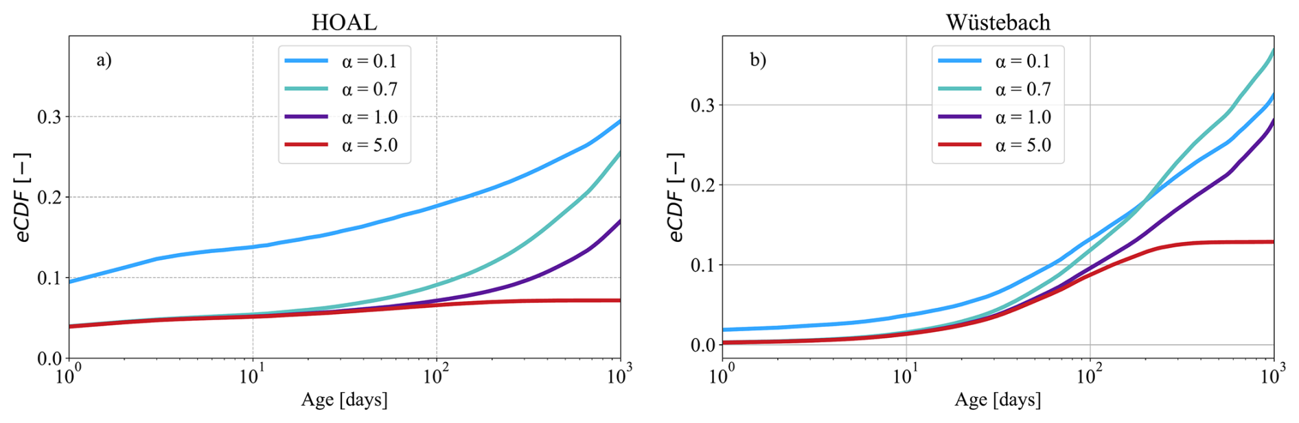
Figure 10 The mean of empirical cumulative distribution functions (eCDFs) of modelled transit times of daily discharge for the (a) HOAL and (b) Wüstebach catchments under varying SAS shape parameters ($\mathit{\alpha }=\mathrm{0.1},\mathrm{0.7},\mathrm{1.0},\mathrm{5.0}$) for groundwater. Lower α values favour younger water, producing younger transit time distributions, while higher α values shift the distribution toward older water. The mean of inferred TTD lines are illustrated with blue, turquoise, purple, and red lines corresponding to α values of 0.1, 0.7, 1.0, and 5.0, respectively. The simulations ranged from very young water preference (α=0.1) to old water preference (α=5) for the groundwater, while for the root zone compartment, a calibrated value was used (α₀=0.14, for HOAL and 0.98 for Wüstebach).

3.6 Variation in the streamflow tracer signal and TTD estimations under different passive groundwater storage volumes and mixing assumptions

The results addressing the extent to which passive storage volume and associated mixing assumptions influence the representation of preferential groundwater flow, the estimated transit time distributions, and the interpretation of tracer signals at the catchment scale, are presented in Figs. 11 and 12. Briefly, the findings show that increasing the passive storage volume dampens the contribution of younger water, shifts the overall transit time distribution towards older ages, and reduces variability in the δ²H signal variability in streamflow.

In both catchments, an active storage volume equivalent to approximately 1 % of the passive storage volume was needed to attenuate the modelled tracer signal in line with observations in streamflow. In the HOAL, a passive storage volume of $S_{\mathrm{S},\mathrm{p}}=\mathrm{500}$ mm (Fig. S10a) was sufficient to attenuate the modelled tracer signal, while in Wüstebach, a much larger volume of $S_{\mathrm{S},\mathrm{p}}=\mathrm{5000}$ mm was necessary (Fig. S10b). SAS shape parameters indicating a young-water preference (α=0.1) resulted in variable δ²H signals in streamflow, whereas an older-water preference (α=5.0) led to stronger dampening (Figs. 11, 12).

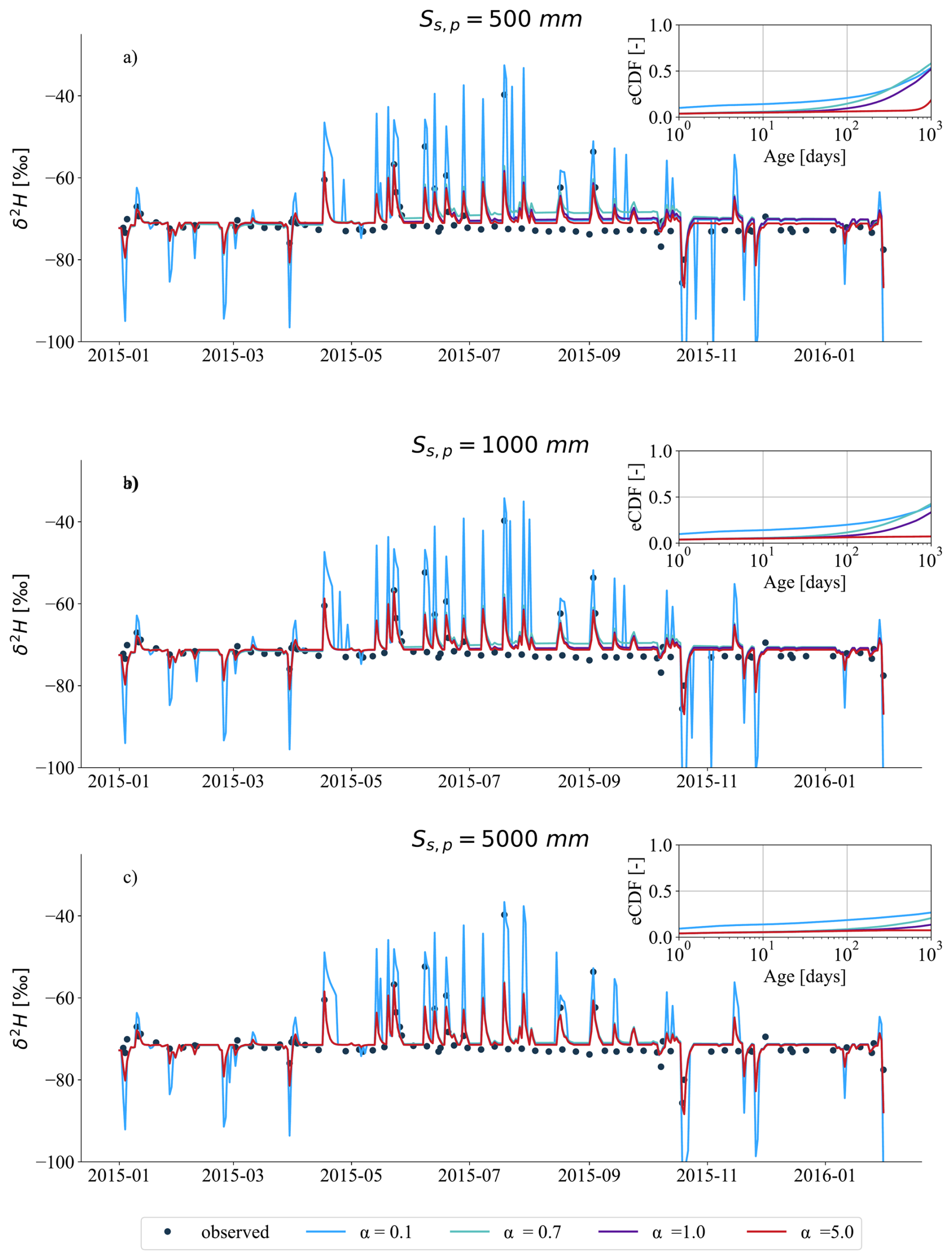
Figure 11 modelled δ²H signals in streamflow (Q; mm d⁻¹) for the HOAL catchment in the year 2015, based on varying passive groundwater storage volumes ($S_{\mathrm{S},\mathrm{p}}=\mathrm{500}$, 1000, and 5000 mm) and different mixing assumptions defined by SAS function shape parameters (α=0.1, 0.7, 1.0, and 5.0). (a–c) Each plot shows results for one S_S,p value, with black dots indicating observed grab samples of streamflow δ²H, and coloured lines representing modelled δ²H under the different α values. The inset in each plot shows the mean empirical cumulative distribution functions (CDF) of modelled daily streamflow transit times during the tracking period (2015–2019); line colours correspond to α values: blue for 0.1, turquoise for 0.7, purple for 1.0, and red for 5.0. Simulations over the full tracking period (2015–2019) are provided in the Fig. S11.

Once the volume ratio between active and passive storage fell below 1 %, further increases in S_S,p had little effect on model performance (Table 2). The NSE remained relatively stable across different S_S,p values, with moderate improvements for α=0.7, 1.0, and 5.0. In contrast, simulations with α=0.1 yielded negative NSE values (Table 2). The highest NSE${}_{{\mathit{\delta }}^{\mathrm{2}}\mathrm{H}}$ values, approximately 0.55, were achieved with α=1.0 and α=5.0 for the HOAL catchment. The results in the Wüstebach catchment exhibited a wider range of NSE values, from −11.25 to 0.22, as S_S,p increased, suggesting that model performance was more sensitive to the size of the passive storage volume than to the shape factor α.

In both catchments, increased passive storage volumes influenced the old tail of transit times ($\mathrm{100}<T<\mathrm{1000}$ d). Increasing S_S,p increased the probability of older water contributing to streamflow (Figs. 11, 12) and reduced the fraction of streamflow younger than 1000 d substantially. The range of differences in the fraction of streamflow younger than 1000 d varied across different mixing assumptions, yet remained consistent overall. In the HOAL catchment (Fig. 11a–c), under the uniform sampling assumption, the fraction of streamflow younger than 1000 d decreased from 50 % to 5 % as S_S,p increased from 500 to 5000 mm. Given that model performance remained similar across these scenarios (Table 2), this implies a variability of approximately 45 % in TTD estimation attributable to uncertainties in passive storage volumes. In the Wüstebach catchment (Fig. 12a–c), the corresponding fraction declined from 80 % to 45 %. None of the simulations with S_S,p less than 5000 mm adequately reproduced the observed δ²H signal, suggesting that at least 50 % of stream water in Wüstebach is older than 1000 d.

Table 2 Performance metrics for modelled δ²H values in the HOAL (from 2015 to 2019) and Wüstebach (from 2011 to 2013) catchments under varying passive groundwater storage volumes (S_s,p) and groundwater SAS function shape parameters (α). For each S_s,p volume (500, 1000, and 5000 mm), simulations were run with α values representing a range from very young-water preference (α=0.1) to old-water preference (α=5.0). The root zone SAS function was fixed at its calibrated value for each catchment (α₀=0.14 for HOAL and 0.98 for Wüstebach). Performance was evaluated using the Nash-Sutcliffe Efficiency (NSE${}_{{\mathit{\delta }}^{\mathrm{2}}\mathrm{H}}$) and Mean Absolute Error (MAE${}_{{\mathit{\delta }}^{\mathrm{2}}\mathrm{H}}$) between observed and modelled streamflow δ²H signals.

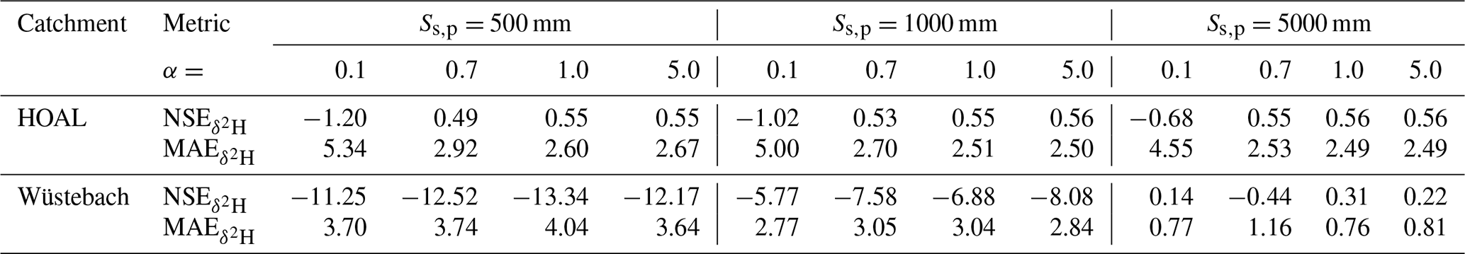
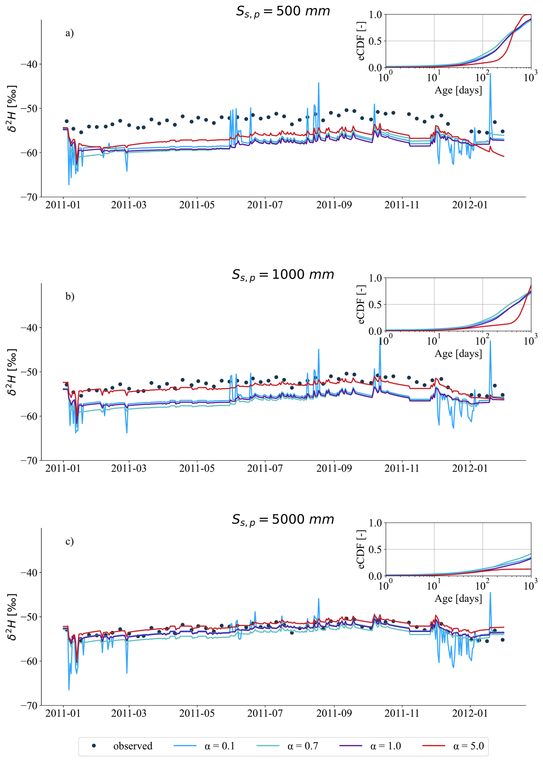
Figure 12 Modelled δ²H signals in streamflow (Q, mm d⁻¹) for the Wüstebach catchment in the year 2011, based on varying passive groundwater storage volumes ($S_{\mathrm{S},\mathrm{p}}=\mathrm{500}$, 1000, and 5000 mm) and different mixing assumptions defined by SAS function shape parameters (α=0.1, 0.7, 1.0, and 5.0). (a–c) Each plot shows results for one S_S,p value, with black dots indicating observed grab samples of streamflow δ²H, and coloured lines representing modelled δ²H under the different α values. The inset in each plot shows the mean empirical cumulative distribution functions (eCDFs) of modelled daily streamflow transit times during the tracking period. Line colours correspond to α values: blue for 0.1, turquoise for 0.7, purple for 1.0, and red for 5.0. Simulations over the full tracking period (2011–2013) are provided in the Fig. S12.

4 Discussion

4.1 Comparison of catchment transit times

The inferred transit times in HOAL (13 % of streamwater younger than 1000 d) and Wüstebach (27 % of streamwater younger than 1000 d) indicated that, in both catchments, the majority of water contributing to streamflow was relatively old, consistent with findings from many other catchments (Kirchner et al., 2023; Floriancic et al., 2024; Wang et al., 2025). During wet periods, the fraction of water T<1000 d was 15 % in HOAL and 33 % in Wüstebach; in dry periods, these values dropped to 10 % and 22 %, respectively. This variation indicated a greater release of younger water under wetter conditions, consistent with other studies (Klaus et al., 2013; Angermann et al., 2017; Loritz et al., 2017). In Wüstebach, relatively high soil wetness and high monthly mean young-water fractions ranging from 5 % to 15 % (Fig. 5e, f) pointed to wet-soil promotion of preferential flow which has been observed previously (Wiekenkamp et al., 2016; Stockinger et al., 2014; Hrachowitz et al., 2021; Hövel et al., 2024). By contrast, HOAL’s younger-water release did not depend on soil wetness only; instead, rapid flow pathways (e.g. infiltration-excess overland flow, macropores, tile drains) as known for this catchment (Exner-Kittridge et al., 2016; Pavlin et al., 2021; Vreugdenhil et al., 2022) allowed water to bypass much of the soil matrix and reach the stream quickly, even under dry conditions, which was discussed in previous findings (Türk et al., 2025; Széles et al., 2020). The consistency of our results with prior tracer-based modeling and SAS applications in both HOAL (Széles et al., 2020; Türk et al., 2025) and Wüstebach (Stockinger et al., 2019; Hrachowitz et al., 2021) provides confidence in the applied model configurations. However, we acknowledge that such consistency alone cannot exclude the possibility of shared assumptions. Therefore, we use these results as supporting evidence that the model setups are reasonable for testing the research hypotheses, while recognizing the need for further validation with complementary data and approaches.

4.2 Do stream water tracer data have sufficient variability to identify preferential flow in the unsaturated root zone and in groundwater using different SAS functions?

Positive correlations between modelled and observed streamflow tracer signals (Fig. 6a, b), together with high model-efficiency metrics at lower α₀ values (indicating a preference for younger water; Table 1), show that streamflow tracer data were sufficiently sensitive to the SAS parameterization of preferential flow in the unsaturated zone for both the HOAL and Wüstebach catchments. This suggests rapid transport of precipitation through preferential flow pathways in both catchments, consistent with previous findings (Wiekenkamp et al., 2016; Stockinger et al., 2014; Széles et al., 2020). Specifically, changing the root-zone SAS shape parameter α₀ produced clear differences in modelled streamflow δ²H signals (Fig. 6), demonstrating tracer-data sensitivity to younger-water release. The results quantitatively demonstrated that streamflow isotope data can reflect the activation of preferential flow in the unsaturated zone. While previous studies have identified preferential flow through field observations (Vreugdenhil et al., 2022; Pavlin et al., 2021; Wiekenkamp et al., 2016), our results demonstrate that they can also be captured and interpreted using catchment-scale tracer modelling.

Nevertheless, the two catchments exhibited distinct processes controlling preferential flow in the unsaturated root zone. The calibrated lower boundary of the SAS function shape parameter, α₀, differed markedly (α₀=0.14 for HOAL and α₀=0.98 for Wüstebach), reflecting contrasting storage-discharge relationships and preferential flow activation mechanisms in the unsaturated zone. In HOAL, the low α₀ value indicated rapid, direct water transmission through preferential flow paths driven by intense rainfall, consistent with previous hydrometric analyses and field observations (Pavlin et al., 2021; Vreugdenhil et al., 2022). This suggests younger water to reach the stream with limited mixing with stored water. This was further facilitated by the formation of soil crusts and cracking of the clay-rich topsoil during the dry summer months, creating direct preferential pathways that accelerate water transmission through the catchment (Exner-Kittridge et al., 2016). In contrast, the higher α₀ value in Wüstebach (α₀=0.98) indicated that under wetter antecedent conditions, established preferential flow pathways promoted greater subsurface mixing, leading to relatively older water contributions to streamflow. This likely reflects the influence of forest cover in Wüstebach, where enhanced infiltration promotes deeper and more uniform mixing (Wiekenkamp et al., 2016) than in HOAL. Despite contrasting site characteristics, both catchments showed responses consistent with previous studies that documented the role of macropores and preferential flow pathways in the unsaturated zone, where water frequently bypasses matrix storage and exchange processes (Zehe et al., 2006; Angermann et al., 2017; Sprenger et al., 2016; Klaus et al., 2013; Loritz et al., 2017).

On the other hand, streamflow tracer δ²H showed limited sensitivity to variations in groundwater SAS function parametrizations (Fig. 8, Table 1), suggesting that isotope data alone may not provide sufficient variability to resolve preferential groundwater flow contributions to streamflow. This is supported by the small variation in correlation coefficient for different α values (r=0.54–0.60 in the HOAL catchment and r=0.71–0.76 in Wüstebach). We attributed this limited variability to the large passive groundwater storage volumes (estimated as 500 mm in HOAL and 5000 mm in Wüstebach;) formulated within the model. The estimated passive groundwater storage volumes should be interpreted as volumes effectively buffering δ²H simulations, rather than their actual physical magnitude. In our and many other catchment scale modelling approaches (Benettin et al., 2015a; Hrachowitz et al., 2013; Wang et al., 2023, 2025), groundwater (Q_S) age selection is formulated based on age samples from the total groundwater storage (S_S,tot), combining contributions from both active (S_S,a) and passive (S_S,p) compartments (Zuber, 1986; Hrachowitz et al., 2015). Thus, the age-ranked groundwater storage (S_T,S,tot) inherently reflected a mixture of these storage volumes. Although the model explicitly allowed preferential recharge of younger groundwater (e.g, R_fs, Fig. 2), the passive storage, characterized by long residence times, buffers the isotopic signals in streamflow (Birkel et al., 2011), result in comparable model performance (Table 2), thereby masking the distinct signatures of preferential groundwater flow. Consequently, uncertainty in estimating passive storage volumes in modelling leads to uncertainty in transit time estimation and contaminant transport time scales, with critical implications for assessing water-quality risks. For water-quality modelling, this implies that rapid contaminant transport through preferential flow paths can occur in response to hydrological events; however, stable water isotope data alone are insufficient to capture these dynamics in catchments with substantial passive groundwater storage.

The Spearman rank correlations (r) between observed and modelled δ²H were lower in HOAL compared to Wüstebach, which can be attributed to differences in temporal resolution and the variability of isotope sampling (Fig. 1a, b). Although model performance metrics, such as NSE or correlation coefficients, quantify the agreement between modelled and observed isotope time series, they can result in seemingly good fits in the presence of sparse or irregular data sampling. In such cases, deceptively high NSE values may still occur even when key groundwater age-selection parameters (e.g., preference for young vs. old water) remain poorly constrained, thereby affecting transit time estimations (Stockinger et al., 2016).

4.3 Does accounting for preferential flow described by a SAS function affect catchment-scale transit time distributions?

Different groundwater SAS function parameterizations yielded similar isotope model fits (Table 2), except for the case with a strong young-water preference (α=0.1) in the HOAL catchment, indicating that good tracer model performance does not necessarily imply well-constrained groundwater age selection. For example, assuming a strong young-water preference (α=0.1) yielded fractions of streamflow younger than 1000 d of approximately 25, % in HOAL and 35, % in Wüstebach, whereas an older-water preference (α=5.0) reduced these fractions to around 5 % and 12 %, respectively (Fig. 10). This spread of 20 % in HOAL and 23 % in Wüstebach for T<1000 d highlights a key limitation of isotope-based model calibration: transit time estimates remain highly uncertain when groundwater mixing processes and SAS function formulations are weakly constrained. This uncertainty is particularly relevant for contaminant transport prediction, as poorly constrained groundwater age distributions can lead to inaccurate estimates of contaminant travel times and the timing of water-quality improvements following reductions in contaminant inputs. Consistent with previous studies (van der Velde et al., 2012; Borriero et al., 2023), our results show that inferred transit times are sensitive to how SAS functions are conceptualized and parameterized, underscoring the need for additional constraints or complementary tracers when interpreting groundwater transit times and their implications for catchment functioning and water-quality assessment.

4.4 How groundwater mixing assumptions and passive storage volumes influence tracer simulation and transit time estimation at the catchment scale?

In both the HOAL and Wüstebach catchments, streamflow isotope signals were attenuated when the volume ratio between active and passive storage ($S_{\mathrm{S},\mathrm{a}}/S_{\mathrm{S},\mathrm{p}}$) was less than 1 % (Figs. 11, 12), indicating that passive groundwater storage volumes orders of magnitude larger than active groundwater storage are required to significantly dampen isotope variability in streamflow, consistent with findings by Birkel et al. (2011).

In HOAL, model performance remained comparable across a wide range of passive storage volumes exceeding 500 mm (e.g., ${\mathrm{NSE}}_{{\mathit{\delta }}^{\mathrm{2}}\mathrm{H}}\approx \mathrm{0.55}$), suggesting uncertainty in the upper bound of passive storage, as model performance became insensitive to further increases once the $S_{\mathrm{S},\mathrm{a}}/S_{\mathrm{S},\mathrm{p}}$ ratio dropped below 1 %. In contrast, model performance in Wüstebach systematically improved with increasing passive storage volumes (Table 2), consistent with previous findings by Hrachowitz et al. (2021), who proposed substantial groundwater storage (∼ 8000 mm) to reproduce observed isotope damping. Nevertheless, the sensitivity analysis demonstrated that similar performance (${\mathrm{NSE}}_{{\mathit{\delta }}^{\mathrm{2}}\mathrm{H}}=\mathrm{0.31}$) could also be achieved with $S_{\mathrm{S},\mathrm{p}}=\mathrm{5000}$ mm under uniform mixing, reinforcing the large uncertainty in constraining the upper range of passive storage volumes in catchment-scale models.

Given these uncertainties in passive storage parameters, it is therefore crucial to assess how passive groundwater storage, in combination with active storage, influences estimated TTDs. In both catchments, a clear negative correlation emerged between passive storage volume and the fraction of streamflow younger than 1000 d (Figs. 11, 12). Because the groundwater storage SAS function was formulated based on the sum of active and passive groundwater storage ($S_{S,\mathrm{tot}}=S_{\mathrm{S},\mathrm{a}}+S_{\mathrm{S},\mathrm{p}}$), increasing passive storage volumes systematically increased the likelihood of older water contributions to streamflow, thereby extending the tails of the transit time distributions (TTDs; $\mathrm{100}<T<\mathrm{1000}$ d). These results underscore that passive groundwater storage is a dominant control on catchment memory (the retention of past hydrological inputs in streamflow due to long residence and transit times), substantially masking young-water contributions and promoting delayed solute and pollutant transport at the catchment scale.

4.5 Implications and limitations

The sensitivity analyses of streamflow tracer signals and transit time estimates to SAS function parameterizations offered a systematic approach that could be adapted to other regions and TTD studies. Nonetheless, the uncertainty resulting from the specific model setup and parameter choices used in this study cannot be directly generalised across diverse catchments or hydrological conditions. Reducing uncertainty in transit time estimates and enhancing the reliability of SAS-based modelling requires improving the spatial and temporal resolution of isotope and hydrological data, integrating additional tracers such as tritium (³H), and refining model representations of subsurface processes.

At the catchment scale, isotope-based modelling proved useful in capturing preferential flow in the unsaturated zone but was limited in doing so in groundwater due to the damping of water stable isotope signals by large passive groundwater storage volumes. This damping does not necessarily indicate the absence of preferential flow; rather, it implies that when isotope variability in streamflow is strongly attenuated, groundwater age mixing will be difficult to constrain using isotopes alone. This limitation is relevant for water-quality applications, as catchments with large passive groundwater storage may still exhibit rapid contaminant responses during hydrological events through preferential flow pathways, despite long mean transit times. Consequently, applying this modelling approach to other catchments requires careful consideration of active-passive groundwater storage dynamics, the parametrization of the SAS function.

While the SAS formulation identifies the statistical signatures of preferential flow in tracer-based modelling, it does not explicitly resolve the physical mechanisms that induce preferential flow. Therefore, isotope data alone, when used within a catchment-scale conceptual model framework, may be insufficient to distinguish between a true absence of preferential flow and a limited model sensitivity to detect it. This limitation of relying on stable isotope data alone is especially critical for water-quality prediction, where preferential flow paths can rapidly mobilize nutrients or contaminants during hydrological events, even in systems characterized by large storage and long mean transit times.

In the HOAL catchment, Exner-Kittridge et al. (2016) showed that alternating contributions from shallow and deep aquifers throughout the year were the main cause of the seasonal variability in nitrate concentrations in streamflow. These alternating contributions, together with extensive tile drainage and heterogeneous clay-rich soils, create rapid and spatially variable flow pathways (Exner-Kittridge et al., 2016; Pavlin et al., 2021).Such features, combined with overland flow in the HOAL catchment (Blöschl et al., 2016), likely favour the activation of preferential flow. For the Wüstebach catchment, field studies indicated that soil and groundwater dynamics are coupled. Bogena et al. (2015) and Graf et al. (2014) showed that soil water variability decreases with depth due to lower porosity and root water uptake in shallow depth, while groundwater fluctuations closely follow soil moisture dynamics (Bogena et al., 2015), reflecting high infiltration and storage capacity in forest soils. This soil-groundwater coupling contrasts with the results obtained in the HOAL catchment, suggesting a more uniform subsurface mixing in Wüstebach.

Although the physical mechanisms underlying preferential flow and subsurface mixing remain beyond the explicit resolution of conceptual, isotope-based transport models, the SAS framework enables delineation of the hydrological conditions under which preferential flow effects become detectable. This capability of the SAS functions is particularly important for identifying when fast flow paths control solute export during extreme events or periods of high hydrological connectivity. Future research should combine stable isotopes with complementary tracers (e.g., tritium, chloride, or major ions) and higher-frequency sampling to enhance the diagnostic power of tracer-aided models. Furthermore, linking SAS function shapes to measurable catchment attributes could enable a priori parameterization, thereby reducing dependence on calibration. At the lysimeter pedon scale, Asadollahi et al. (2020) showed that SAS functions can approximate the analytical solution of the advection-dispersion equation; however, extending such mechanistic relationships to the catchment scale remains challenging within conceptual modelling frameworks.

While our study focused on a conceptual catchment-scale framework, the results highlighted the need to advance toward more distributed models that can more directly link spatial heterogeneity in soils, slopes, and storage to preferential flow dynamics. Addressing these challenges represents a key step toward integrating empirical SAS modelling with a process-based interpretation of preferential flow and improving predictions of solute transport and water-quality responses, particularly under event-driven activation of preferential flow in the subsurface.

5 Conclusions

In this study, we evaluated whether stream water isotope data contain sufficient variability to simulate preferential flow in the unsaturated zone and in groundwater aquifers. By testing various StorAge Selection (SAS) function parametrizations within a catchment-scale transport model, we analysed the effects of explicitly representing preferential root-zone and groundwater flow on the estimation of transit time distributions (TTDs). The findings indicated that streamflow tracer data were sufficiently sensitive to the SAS parameterization of preferential flow in the shallow unsaturated zone; however, they were insufficient to constrain SAS parameterizations for groundwater due to the strong damping effect of passive groundwater storage on isotopic variability, leading to uncertainty in catchment TTD estimates. The main findings of our study are:

• Streamflow isotope (δ²H) data were sensitive enough to characterise preferential flow processes in the unsaturated root zone, confirming that such processes significantly shape catchment isotope signatures and transit time distributions at short timescales (up to 300 d).

• Streamflow isotope data alone were insufficient to differentiate among groundwater SAS function shapes for the two tested catchments. Large passive groundwater storage volumes significantly dampened isotopic variations, making it impossible to isolate preferential flow in groundwater.

• The variability in groundwater TTD estimates arising from varying SAS function shapes for groundwater was considerable (20 % for HOAL and 23 % for Wustebach across tested SAS parameterizations), highlighting that TTD estimates are sensitive to how SAS functions are conceptualised and parameterised within the model.

• The size of the passive groundwater storage exerts a dominant control on catchment transit time estimates, particularly influencing the longer tails (T>100 d) of the distributions, thereby introducing uncertainties in the timing of solute and contaminant transport.

These findings have implications for solute and contaminant transport timescales within catchments, in addition to the estimation of water transit times. Large passive groundwater storage volumes imply prolonged retention times, potentially delaying the transport and release of pollutants. The uncertainty in estimating passive groundwater storage volumes translates into uncertainty in contaminant transport predictions, with critical implications for assessing water-quality risks. Additional or complementary datasets, such as direct groundwater measurements or higher-frequency tracer sampling, are likely required to characterise preferential groundwater flow using conceptual, catchment-scale transport models. Improved characterisation of passive groundwater storage volumes, potentially through complementary observations (e.g., groundwater level monitoring or high-frequency isotope sampling), is essential to reduce uncertainties and enhance reliability in transit time and solute transport modelling at the catchment scale.