The importance of model horizontal resolution for improved estimation of snow water equivalent in a mountainous region of western Canada

Accurate estimation of snow water equivalent (SWE) over high mountainous regions is essential to support water resource management. Due to the sparse distribution of in situ observations in these regions, weather forecast models have been used to estimate SWE. However, the influence of horizontal resolution on the accuracy of the snow simulation remains poorly understood. The objective of this study is to evaluate the potential of the Weather Research and Forecasting (WRF) model run at horizontal resolutions of 9, 3, and 1 km to estimate the daily values of SWE over the mountainous South Saskatchewan River Basin (SSRB) in western Canada for a representative water year, 2017–2018. Special focus is given to investigating the impact of the WRF model grid cell size on accurate estimation of the peak time and value of SWE across the watershed. Observations from manual snow surveys show an accumulation period from October 2017 to the annual peak in April 2018, followed by a melting period to the end of water year. All WRF simulations underestimated the annual SWE. The largest errors occurred in two conditions: at higher elevations and when using coarser horizontal resolution. These biases reached up to 58 kg m⁻² (24 % relative error). The two higher-resolution simulations capture the magnitude (and timing) of peak SWE very accurately, with only a 3 % to 6 % low bias for 1 and 3 km simulations, respectively. This demonstrates that a 1 km resolution may be appropriate for estimating SWE accumulation across the region. A relationship is identified between model elevation bias and SWE biases, suggesting that the smoothing of topographic features at lower horizontal resolution leads to lower grid cell elevations, warmer temperatures, and lower SWE. Overall, this study indicates that high-resolution WRF simulations can provide reliable SWE values as an accurate input for hydrologic modeling over a sparsely monitored mountainous catchment.

1 Introduction

On average, almost 65 % of Canada's landmass is covered by annual snow cover for more than 6 months of the year (ECCC, 2025). Melting snow in spring is a critical component of the water cycle to determine water supplies and flood risk; however, estimating the effect of snowmelt on flooding depends on a reliable estimate of snow water equivalent (SWE) (Dozier et al., 2016; Wrzesien et al., 2017; Vionnet et al., 2020). SWE is defined as the product of snowpack depth and bulk density and is a key environmental variable for understanding climate (Brown et al., 2019). It represents the vertical depth of water that would be obtained if all the snow cover melted completely (WMO, 2018). The value of SWE shows the amount of liquid water which is produced from a melting snowpack.

The distribution of SWE across space and time is especially important in northern regions and at high elevations. This distribution determines how much water will be available during spring and summer runoff periods (Barnett et al., 2005; King et al., 2020). Due to the sparse distribution of in situ observations globally, regional weather forecast models have been used recently to estimate the amount of SWE (Klehmet et al., 2013; Wrzesien et al., 2017; Raparelli et al., 2023). Reliable and accurate estimation of SWE has been required to improve management and analyses of water resources. It is also essential for other applications, including global change analysis and risk assessment (Taheri and Mohammadian, 2022). Although many studies have evaluated temperature and precipitation simulations over North America (Diaconescu et al., 2016; Xu et al., 2019; Holtzman et al., 2020), few studies have been performed regionally to validate the model estimation of the spatial and temporal patterns in SWE (e.g., Alonso-González et al., 2018; Mortezapour et al., 2020). There is ample evidence from previous studies that model horizontal resolution is one of the key factors that should be improved to increase the accuracy of a simulated snowpack (Blöschl, 1999; Leung et al., 2003). Regional climate simulations using a coarse horizontal grid spacing typically underestimate the snowfall compared to the observations. One specific example showed that reducing the MM5 model (fifth-generation Penn State–NCAR Mesoscale Model) grid spacing to 13 km led to an improved estimation of the snowpack for the western United States (Leung and Qian, 2003). Garvert et al. (2007) found that a high-resolution mesoscale model is required to appropriately simulate the snowfall over a complex terrain and to produce updraft and downdrafts that had a significant impact on the snowfall patterns. WRF (Weather Research and Forecasting) model simulations at 2 km grid spacing for the Colorado Rocky Mountains are analyzed by Rasmussen et al. (2011). The estimations are verified using Snowpack Telemetry (SNOTEL) data. Their results show that the model successfully simulated spatial and temporal patterns of SWE over the region.

The Rocky Mountains in the USA and Canada stretch from the northernmost part of western Canada to northern New Mexico in the southwestern United States. The eastern slopes of the Canadian Rocky Mountains make up a complex region, and several factors such as season, vegetation, and topography control the discharge of headwater streams from high-elevation catchments to valley bottoms (Hauer et al., 1997). Our study region comprises the eastern foothills region of the Rocky Mountains and the mountain headwaters region of the South Saskatchewan River Basin (SSRB) (see Fig. 1) and it is more focused on the western SSRB region, which includes mountainous areas of the SSRB. The SSRB in western Canada is a major agricultural basin of Canada with a semi-arid climate that is highly dependent on surface water (Martz et al., 2007), which mainly comes from the spring snowmelt (Tanzeeba and Gan, 2012). The SSRB is a major sub-basin of the Nelson River Basin of Canada, rising from the Rocky Mountains in the west and extending eastward through southern Alberta (Tanzeeba and Gan, 2012). The watershed has a sub-humid to semi-arid continental climate. Temperatures can reach 40 °C during the summer and −40 °C during winter (Martz et al., 2007). During the wintertime, precipitation is principally in the form of snow. Most of the annual runoff (around 70 %) of the rivers in this region is supplied from the Rocky Mountains and the foothills (Ashmore and Church, 2001). Annually SSRB accounts for nearly 57 % of the total water allocated in Alberta. The surface water supply in SSRB region mainly comes from the spring snowmelt (Tanzeeba and Gan, 2012), which makes it highly suitable to study the variability of SWE and its potential hydrologic impact.

The main objective of this paper is to evaluate the potential of Weather Research and Forecasting (WRF) model run at various resolutions to correctly simulate the daily values of snow water equivalent (SWE) over the SSRB region. To pursue this objective, in situ observations of snow using the Canadian historical Snow Water Equivalent (CanSWE) dataset are used to evaluate the potential of WRF to detect the variability in SWE. Particular attention is paid to investigating the role of the WRF model's grid cell size in the accurate estimation of peak SWE timing and value across the watershed. The impact of elevation has been also examined by evaluating several statistical diagnostics.

This paper is organized as follows. Section 2 includes the details about the study region as well as an introduction to the WRF model, ERA5, ERA5-Land, and the CanSWE dataset. Section 3.1 analyzes the area-averaged temporal evaluation of WRF SWE and quantifies bias and errors between WRF, ERA5, ERA5-Land, and the CanSWE dataset throughout the study period. Section 3.2 presents WRF SWE spatial evaluations for individual stations using statistical metrics to provide insights into the probable impact of elevation on biases, which is studied in Sect. 3.3. A summary and conclusions are provided in Sect. 4.

2 Data and methodology

2.1 CanSWE dataset

In situ observation of SWE has been widely used in many applications including water and flood forecasting, climate studies, and evaluation of numerical weather prediction models. SWE can be measured manually or automatically as the mathematical product of snow depth and density. The methods that are widely used to measure SWE include snow cores, snow pits, and snow pillows (Elder et al., 1998; Andreadis and Lettenmaier, 2006; Dixon and Boon, 2012). Snow pits and snow courses are manual methods and rely on interpolation to characterize snow depth. This may lead to some errors if snow depth is variable (López-Moreno et al., 2011). However, snow pillows, measuring SWE by weighing the mass of a snow column, are the most common automatic method for continuous monitoring of SWE at a fixed location. They provide valuable time series of snow, despite the fact that they are spatially sparse and expensive to install and maintain (Johnson and Marks, 2004).

The Canadian historical Snow Water Equivalent dataset (CanSWE) combines manual (snow surveys) and automated (includes snow pillows and passive gamma sensors) pan-Canadian SWE observations (Vionnet et al., 2021). This new dataset replaces the Canadian Historical Snow Survey (CHSSD) dataset (Brown et al., 2019) by correcting the metadata, removing duplicate observations, and controlling the quality of the records. In Canada, the majority of in situ SWE measurements are collected by provincial or territorial governments and hydropower companies and their partners. CanSWE dataset was compiled from 15 different sources and includes SWE information for all provinces and territories measuring SWE from 2607 locations across Canada over the period from 1928 to 2020. More details on this dataset are provided by Vionnet et al. (2021).

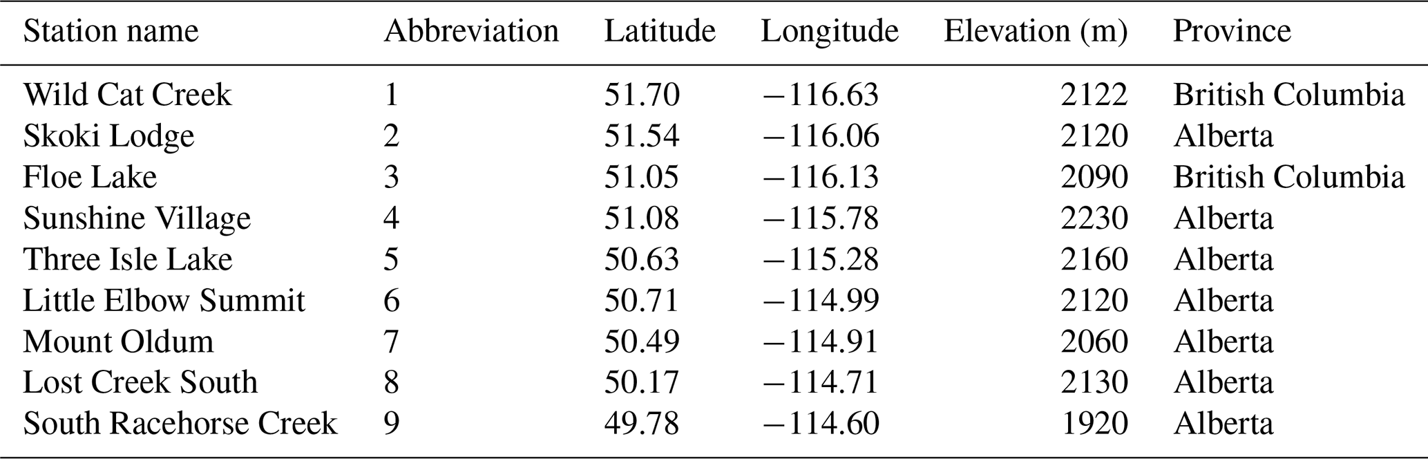
Table 1 shows the location of stations selected to evaluate WRF model performance. Nine weather stations, equipped with automated snow pillows, have been selected based on the availability of daily SWE data with minimal data gaps during the study period. These stations were located over the area represented by the innermost WRF model domain. The evaluation was conducted from 1 October 2017 to 1 October 2018, as the 2018 water year. Our preliminary investigation shows that the 2018 water year had approximately average SWE values during 1984 to 2021 according to the CanSWE stations. Therefore, 2018 can be representative of the region's climate over the past 38 years. Statistical metrics were considered to evaluate the model simulations against CanSWE data: root mean squared error (RMSE), mean bias (MB), mean absolute error (MAE), and standard deviation (SD). The evaluation has been done for each station as well as the aggregate of the stations by examining SWE time series and their annual and spatial distribution.

Table 1 Location of the stations from CanSWE in British Columbia and Alberta.

2.2 WRF model configuration

The Weather Research and Forecasting (WRF) model was developed by the National Center for Atmospheric Research (NCAR) to support both operational weather forecasting and atmospheric research. Detailed documentation of the WRF model can be found in Skamarock (2008). In this study, the Advanced Research WRF (ARW) version 4.3.2 is used with three one-way nested domains, each with progressively finer horizontal resolution. The outer domain has a resolution of 9 km and covers most of western Canada (Fig. 1). The middle domain, with a resolution of 3 km, extends over British Columbia and parts of Alberta. The innermost domain has the highest horizontal resolution of 1 km and covers the western part of the southern Saskatchewan River Basin (Fig. 1). This version of WRF runs with 38 vertical levels between the Earth's surface and a model top at 50 hPa, which is the same for all domains. For the remainder of this paper, the WRF simulations at 9, 3, and 1 km resolutions will be referred to as WRF9K, WRF3K, and WRF1K, respectively. The initial and lateral boundary conditions are derived from the 3-hourly and 0.25° resolution ERA5 reanalysis (Hersbach et al., 2020) from the European Centre for Medium-Range Weather Forecasts (ECMWF). Simulation results are output at a 6 h time step, which is aggregated to daily frequency for direct comparison with observations.

The physical parameterization schemes are selected based on previous studies that employ the WRF model to evaluate the simulation of terrestrial snow accumulation over the Northern Hemisphere (e.g., Niu et al., 2011; Wrzesien et al., 2015; Liu et al., 2017; Li and Li, 2021). In particular, the Thompson et al. (2008) cloud microphysics scheme, the rapid radiative transfer model longwave scheme (Mlawer et al., 1997), the Dudhia shortwave scheme (Dudhia, 1989), the Yonsei University planetary boundary layer scheme (Hong et al., 2006), the modified Kain–Fritsch convective parameterization for the outer domain (Kain and Fritsch, 1990, 1993; Kain, 2004), and the Noah LSM with multi-parameterization (Noah-MP) option (Niu et al., 2011) are used here. Previous studies show that Noah-MP simulates snow more accurately at finer resolution than previous versions of the Noah land surface model (e.g., Wrzesien et al., 2015). Simulated values were extracted at the nearest grid cell corresponding to the location of each station, assuming that the in situ observation is representative of a model gridded area. It is acknowledged that such point comparisons of SWE are inherently challenging due to the heterogeneity in elevation, aspect, and land cover (Cui et al., 2023). However, given the reasonably representative station density within the innermost WRF domain (Fig. 1), we attempt to mitigate these issues by also comparing simulated and observed spatial mean SWE using a spatial mean taken over all stations.

The evaluation of WRF results in the current study has been focused on a discussion of the innermost domain that includes the eastern foothills region of the Rocky Mountains and the mountain headwaters region of the SSRB (Fig. 1). We emphasize that this innermost domain is simulated at all three resolutions; in other words, at each resolution the model produces output over its entire domain, not just the outer part.

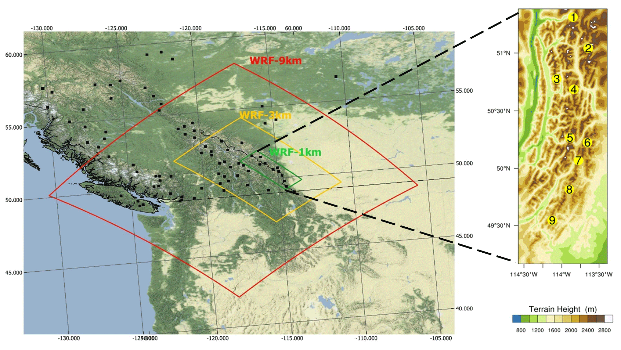
Figure 1 WRF model domains over western Canada and the terrain height for the inner domain. The outer boundaries of the 9 km (red), 3 km (yellow), and 1 km (green) domains are indicated by rectangles. Black squares indicate the location of CanSWE automated stations in British Columbia and Alberta. The topography of the 1 km domain is shown magnified on the right with the CanSWE stations from Table 1 indicated by yellow circles (NCAR Command language version 6.6.2 was used to generate the figure; http://www.ncl.ucar.edu/, last access: January 2025).

2.3 ERA5 and ERA5-L

The datasets used in this study also included ERA5 and ERA5-Land (hereafter, ERA-L) to explore the consistency of the ERA5 and ERA5-L reanalysis datasets in the SWE estimation. As mentioned in Sect. 2.2, the 0.25° resolution ERA5 reanalysis has been also used as the initial and lateral boundary conditions for the WRF run. ERA5 is the fifth-generation ECMWF atmospheric reanalysis (Hersbach et al., 2020) and has a grid resolution of 31 km. This is higher resolution than in the older ERA-Interim of 80 km. ERA5 is based on advanced modeling and data assimilation systems, i.e., the Integrated Forecasting System (IFS) Cycle 41r2, and combines large numbers of historical observations into global estimates. It provides hourly fields for all variables. ERA5 assimilates snow properties from several SYNOP stations, and from the year 2004 onwards, it also uses Interactive Multisensor Snow and Ice Mapping System (IMS) data over the NH (Hersbach et al., 2020). On the other hand, ERA5-L is the land component from ERA5 with a finer spatial resolution of 9 km. It is produced with the land model H_TESSEL and without coupling the atmospheric module without data assimilation (Muñoz-Sabater et al., 2021). These reanalysis data are used to evaluate their SWE values and to understand the role of resolution in SWE estimation over the region.

3 Results

3.1 Evaluation of the spatial mean SWE

The time series of daily SWE values from CanSWE, ERA5, ERA5-L, and WRF simulations averaged over the inner domain of the SSRB are presented in Fig. 2. The results suggest that, on average, improved resolution improves SWE estimation. The seasonal cycle of SWE in observations shows a clear accumulation period from 1 October to peak SWE (648 mm) in late April and a melting period from late April until late June. In general, this seasonal evolution of the snowpack is well represented by the WRF simulations at all three resolutions as well as the reanalysis ERA5 and ERA5-L. However, in agreement with previous studies (e.g., Wrzesien et al., 2018), our results confirm that the reanalysis products significantly underestimate mountain SWE. The ERA5-L SWE at 9 km resolution performs worse than the WRF9K simulation. The peak SWE occurs on the same day, 22 April, for all WRF resolutions and the CanSWE observations, indicating that the WRF model is conserving the primary details of the meteorological lateral boundary forcing required for snow accumulation and melt. The two higher-resolution simulations (3 and 1 km) capture the magnitude of peak SWE very accurately, with only a 3 % to 6 % low bias for WRF1K and WRF3K over the accumulation period, respectively. This demonstrates that both simulations may have value for providing accurate estimates of average SWE accumulation across the study region. The disparity between the CanSWE-SD and estimated-SD of each dataset highlights their inconsistency (Fig. 2). The lowest SDs were associated with WRF1K, which indicates a relatively smaller spread between the WRF1K and CanSWE dataset, suggesting relative consistency and less variability in their values. The WRF9K simulation displays a systematic low bias of about 108 mm (31 %) in SWE throughout the accumulation period, suggesting that either there is too little total precipitation reaching the surface at this resolution, or a temperature bias is causing a lower proportion of precipitation to fall as snow. We examined how temperature and precipitation affect SWE simulations at different resolutions. Temperature values were very similar across all three resolutions (Fig. 3a). However, the WRF9K consistently showed lower precipitation values than expected (Fig. 3b). This suggests that the underestimation of precipitation, rather than temperature differences, is the main cause of SWE bias in the lowest-resolution model. The WRF simulations are configured using a 3-hourly ERA5 forcing at the lateral boundary (i.e., the boundary of the 9 km domain). Therefore, the fact that the WRF9K produces lower total accumulated precipitation than the two higher-resolution simulations over a mountainous region strongly suggests that the cause is orographic enhancement of precipitation within WRF. Interestingly, given that all three of our domains have higher resolutions than ERA5 itself (27 km), this implies that underestimated orographic enhancement may be contributing to a low bias in precipitation at high elevations in ERA5, which in turn leads to a low bias in SWE (Fig. 2).

Figure 2 also shows that the WRF simulation at all three resolutions estimates the melting period in two phases: a rapid phase from April to early June and then a more gradual phase until late June. Also, the difference in melt rate between the two phases is most apparent at the lower resolutions, indicating that melt processes may be more accurately represented at higher resolution based on the melting rate.

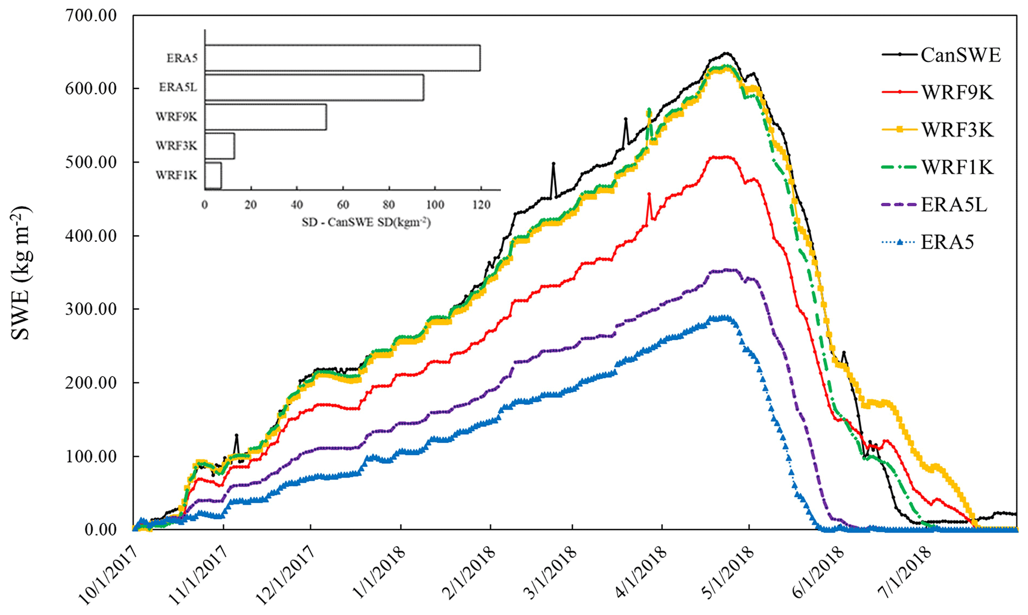
Figure 2 Temporal variation of SWE from CanSWE data, WRF model resolutions, ERA5L, and ERA5 over the SSRB region. The SWE data are aggregated for all stations inside the innermost domain. The spikes in the graph correspond to snowfall events, indicating the accumulation and subsequent melting of snow. The difference between CanSWE SD and the SD of each dataset is shown in the upper left.

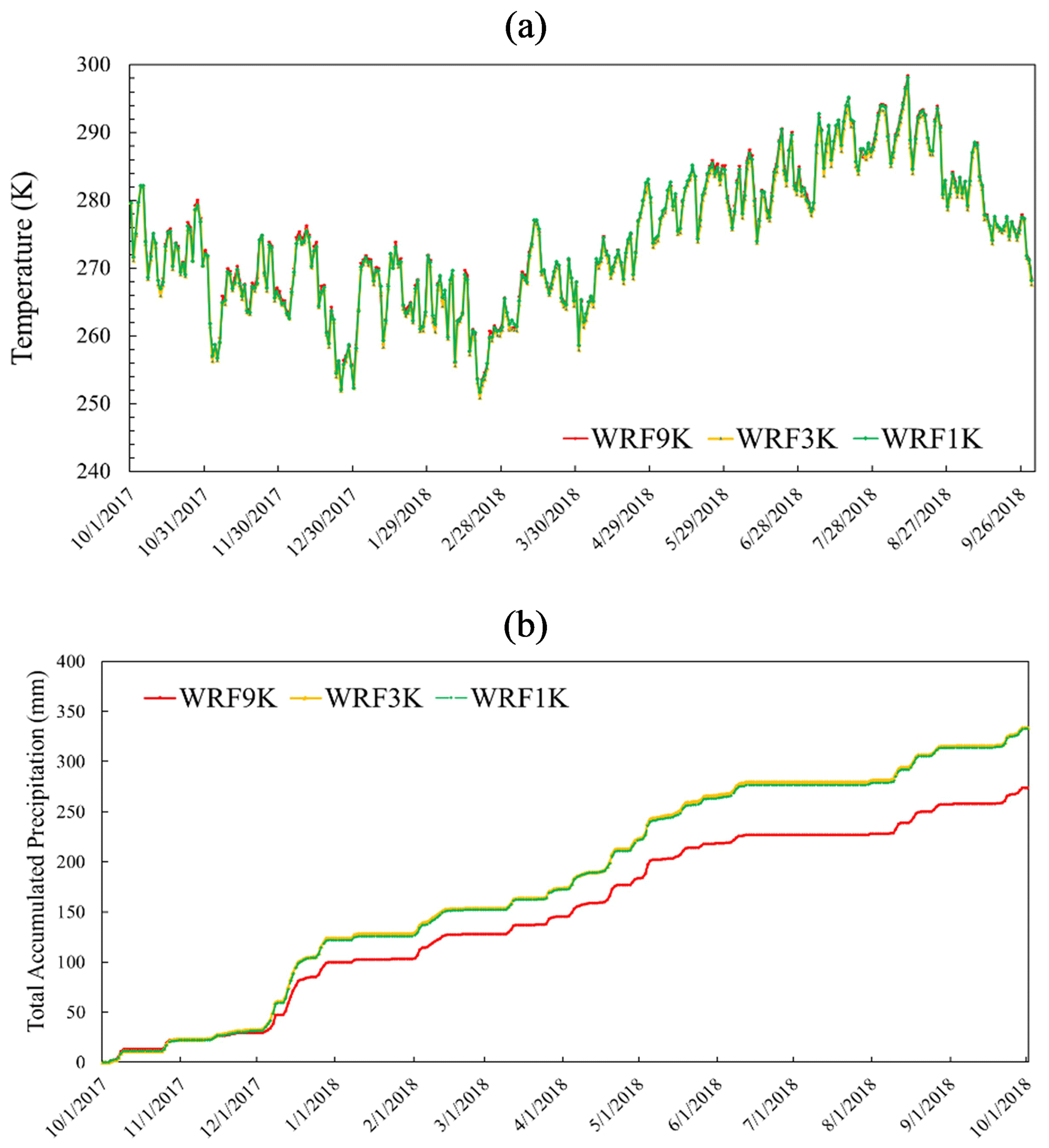
Figure 3 Temporal variation of 2 m temperature (a) and precipitation (b) from the three WRF model resolutions over the SSRB region for the innermost domain.

Summary statistics for the melting and accumulation period are shown in Fig. 4 for RMSE, MB, MAE, and SD over the region. Generally, Fig. 4 suggests that there is tendency for RMSE, MB, MAE, and SD to decrease at finer resolutions. Following ERA5 with 27 km and ERA5-L with 9 km resolution, the coarsest model run shows a high value for RMSE, especially during the accumulation period. WRF9K underestimates SWE values more than the other two finer resolutions during both understudied periods, perhaps due to the incapability of WRF9K to simulate the processes that are responsible for snow redistribution and deposition in mountainous areas that are characterized by heterogeneous snow distribution. Lower error metrics in WRF3K and WRF1K show the effect of the model's scale on the estimation of SWE, leading to biases in SWE simulation. The standard deviation values indicate that, overall, the variance of the estimation differs from the observations; however, there is a trend of decreasing SD with finer resolution, such as in WRF3K and WRF1K. The decrease in SD aligns with lower MAE, RMSE, and bias in WRF1K SWE estimation.

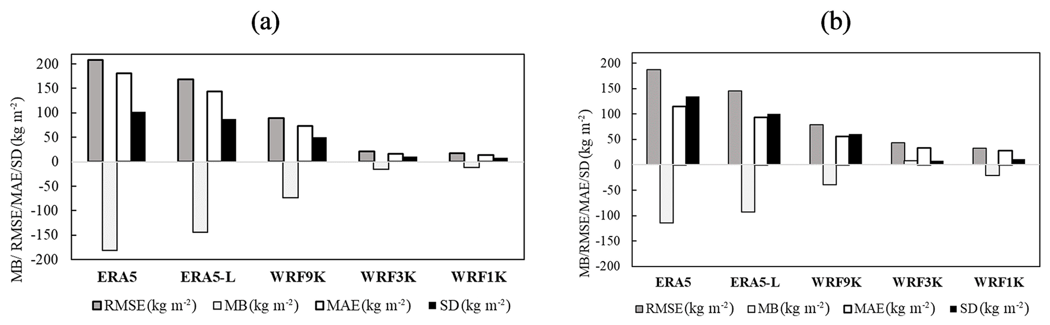
Figure 4 SWE evaluation during the (a) accumulation period (1 October 2017–22 April 2018) and (b) melting period (23 April 2018 to 1 October 2018) over the inner WRF model domain using RMSE, MB, MAE, and SD.

3.2 Evaluation of spatially varying SWE

In this section, the representation of spatial heterogeneity of SWE in the WRF simulations is evaluated by comparing observed and simulated SWE at individual stations within the inner domain. It is important to highlight that the point-to-grid data comparison may introduce uncertainties in the verification results for individual stations. In this context, the emphasis is on the spatial heterogeneity of SWE estimation rather than asserting WRF's accuracy in estimating SWE at a specific point scale. To evaluate the SWE spatial variability, time series for each individual station are depicted in Fig. 5. Moreover, the elevation at each station and the estimated elevation by WRF simulation at all three resolutions are summarized in Table 2. Mostly at the stations on the leeward side of the mountains, including the four southern stations, there is an underestimation of SWE for all runs. At most stations, the WRF run with the finest resolution shows the best performance. SWE experiences significant changes in both space and time; therefore, the accumulation and the snowpack melting are variable because of the complex topography. During the accumulation period, the difference is more pronounced at each station. Comparison between Figs. 2 and 5 shows that aggregation of the stations may smooth the differences between estimations and observations. This effect that is previously introduced by Blöschl (1999) as aggregation filtering may be caused by the change of scale due to the aggregation.

Figure 5 Estimation of SWE using WRF compared to the CanSWE data for stations 1 to 9.

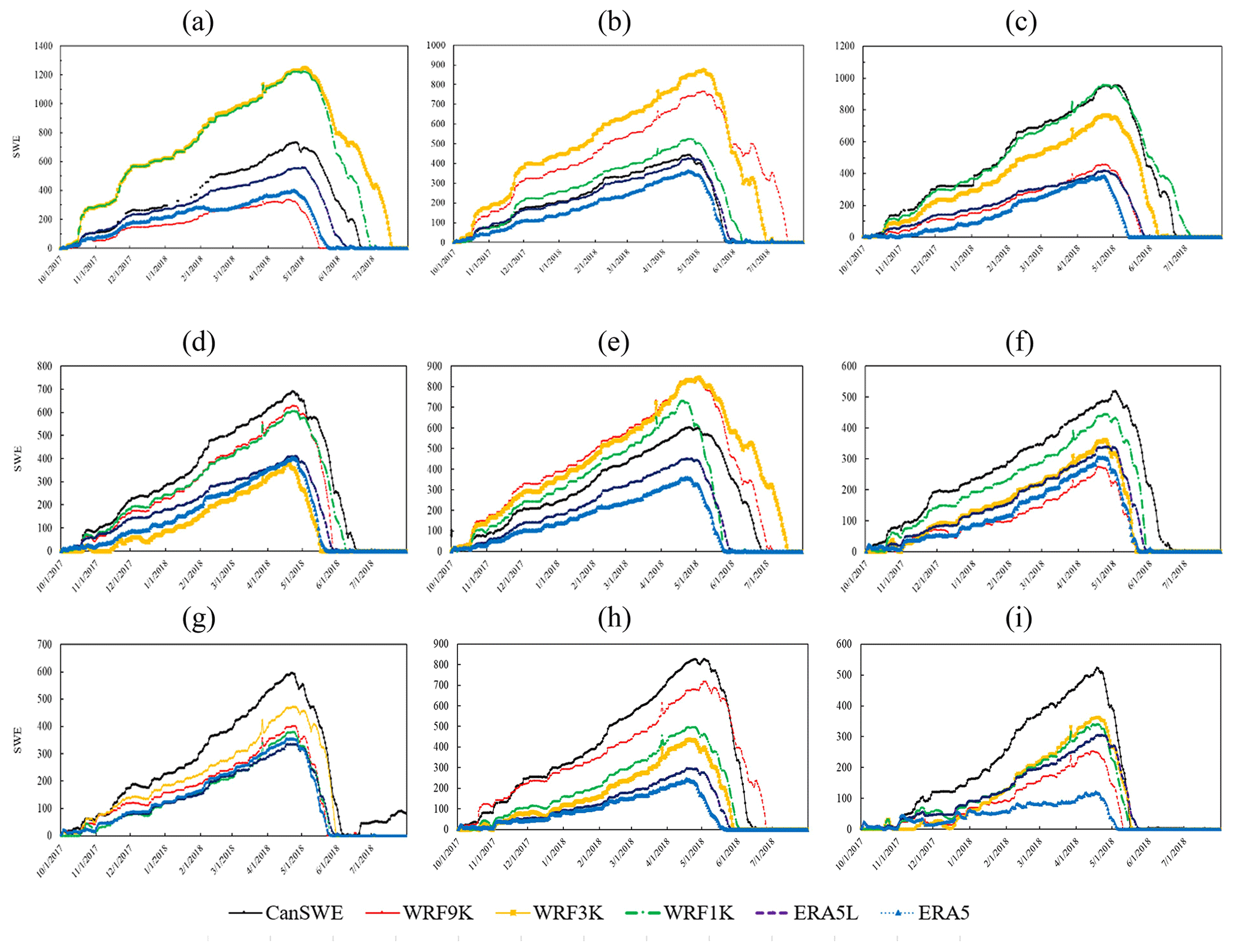
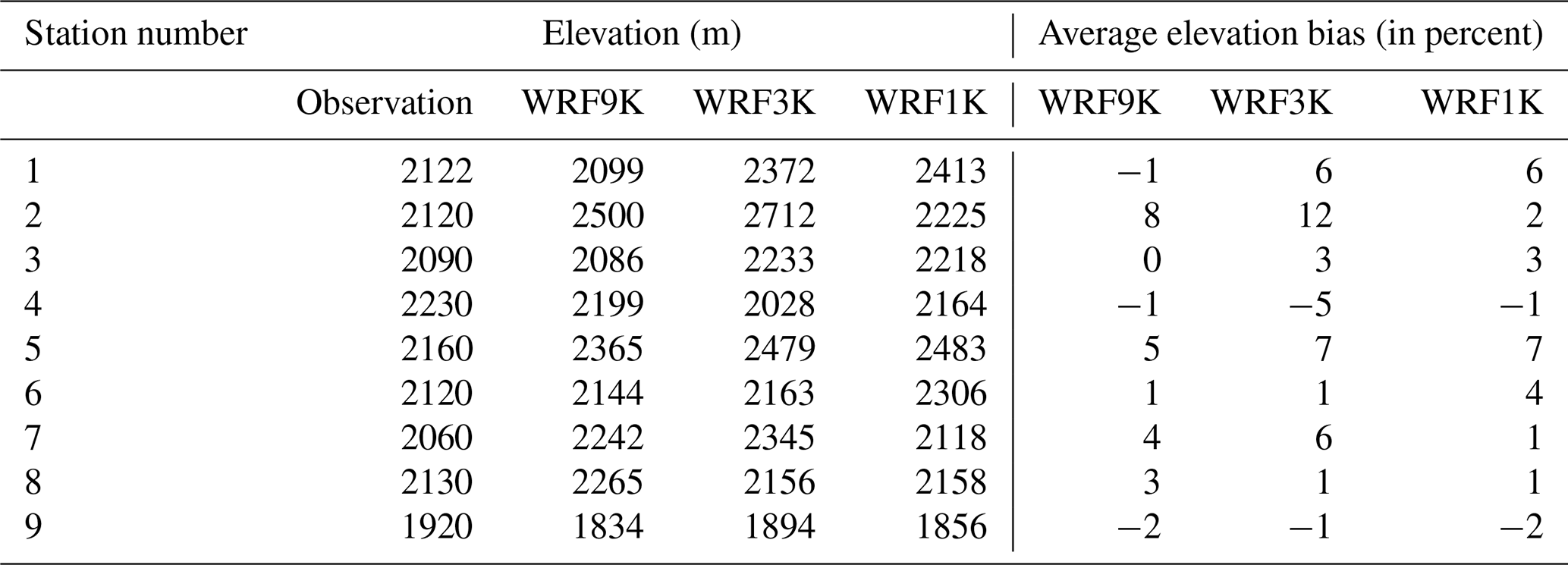
Table 2 Observed elevation of each station vs. the estimated elevation by WRF. Average elevation bias is presented in percent.

The spatial distribution and extent of the SWE for each WRF horizontal resolution are shown in Fig. 6a–f for the accumulation and melting period. As shown in Sect. 3.1, snow accumulates in the mountains from October through April, and snowmelt usually begins in May. The spatial variability in SWE is influenced by various processes occurring across different spatial scales. For example, spatial variability in snow accumulation in mountainous regions may result from the preferential deposition of snow in microscale topographic depressions (Clark et al., 2011). Winds cause the redistribution of snow in the alpine zone, with scouring on the windward side of ridges and deposition on the leeward side (Clow et al., 2012). Both periods show similar spatial distribution of SWE; however, the impact of resolution is obvious. There is a maximum in SWE value in all three simulations over northern parts of the domain for both the accumulation and melting period. During the accumulation period, WRF1K has larger SWE values compared with WRF9K in most areas.

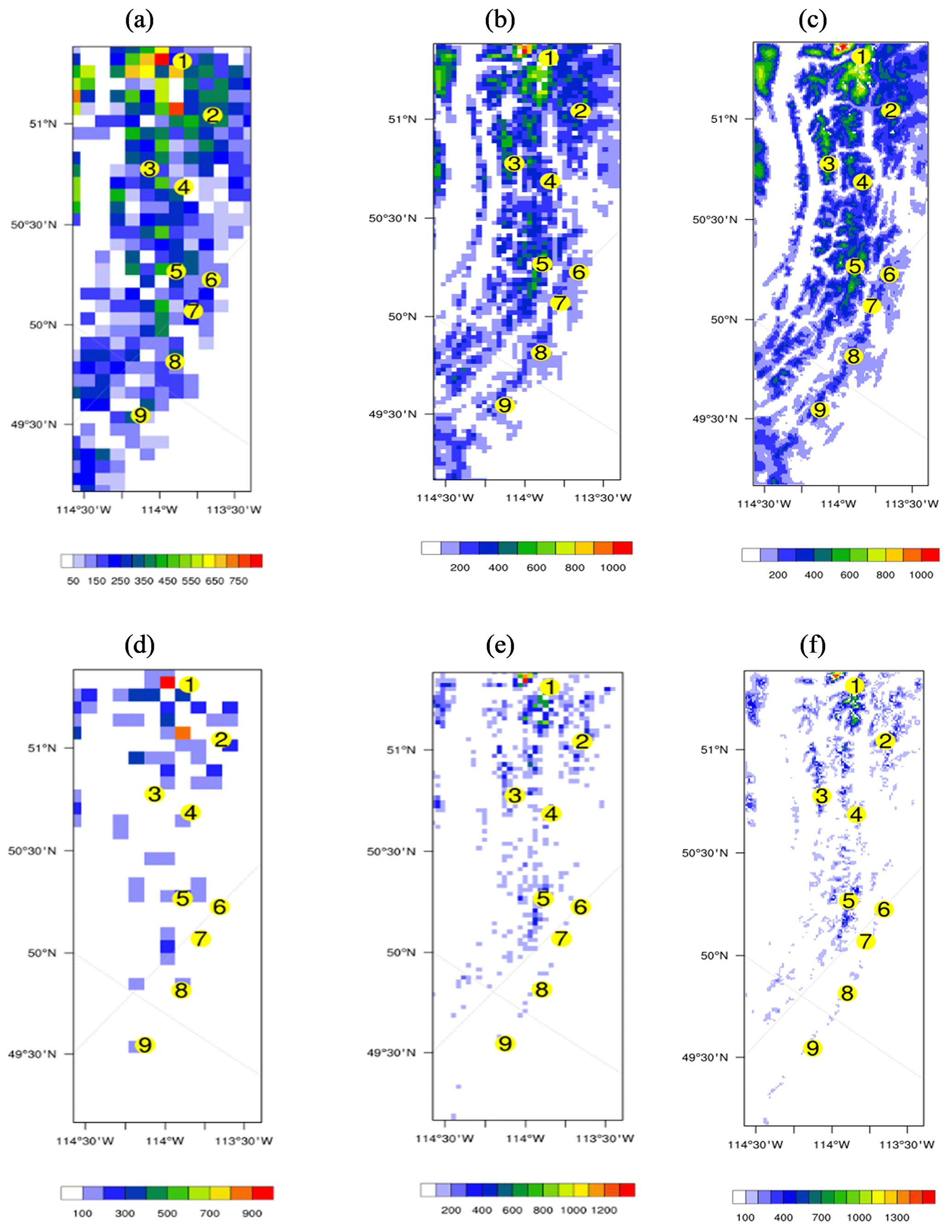
Figure 6 Simulated mean SWE (kg m⁻²) during the accumulation (1 October 2017–22 April 2018) and melting (23 April 2018 to 1 October 2018) period for WRF9K (a, d), WRF3K (b, e), and WRF1K (c, f) over the inner model domain.

To show the errors of the estimates spatially, RMSE, bias, MAE, and SD for each station are compared in Fig. 7 for the accumulation and melting periods. This indicates a geographic sensitivity to bias and errors. Both rms and mean absolute errors show that the estimates are more accurate in the southern portion of the domain, where there is also a negative bias. Result implies that during the melting period, model horizontal resolution becomes critical and there is a substantial SWE underestimation with coarser resolution. Large differences in SD occurred during the melting season; however, at most of the stations WRF1K performs better than the other two resolutions. Factors such as snow drifting, wind scour, and falling debris may also affect patterns and produce different melt rates during the melting period (Dressler et al., 2006).

There are a number of factors that complicate SWE estimation spatially. Spatial variability of the environment, including elevation, slope of the mountain, and boundary roughness, changes continuously from place to place and therefore greatly affects the SWE estimation (Blöschl, 1999; Rice and Bales, 2010). In the following section, results are analyzed to investigate the role of the terrain elevation in explaining the model errors and biases in SWE simulation.

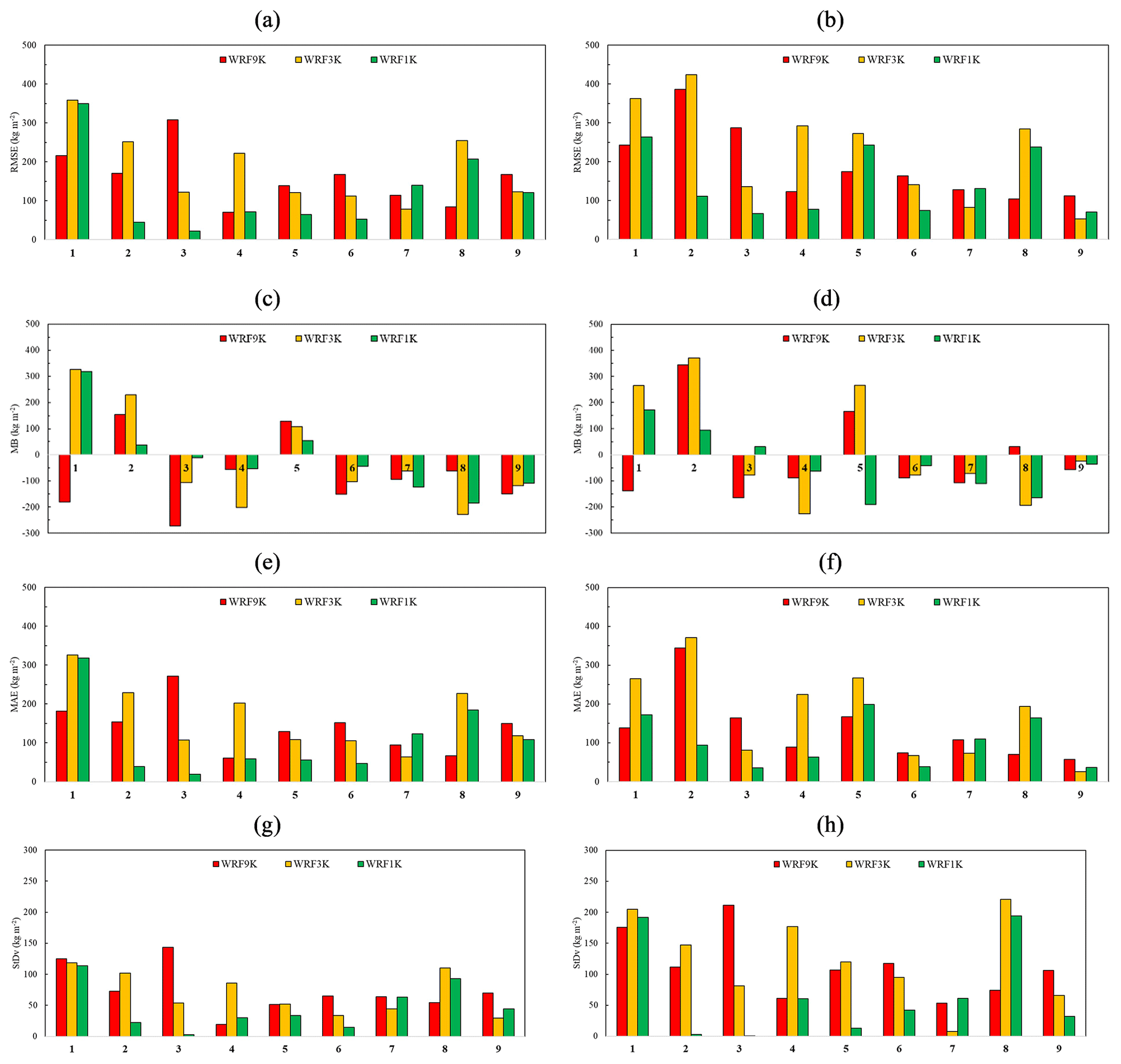
Figure 7 Evaluation metrics for each station including RMSE (a, b), MB (c, d), MAE (e, f), and SD (g, h) for the accumulation (a, c, e) and melting (b, d, f) period.

To study the ability of the WRF model to estimate the date and the value of peak SWE at each station, Table 3 and Fig. 8 evaluate the estimated peak SWE date and values, respectively. Late April to early May 2018 is an approximate estimation of the peak SWE date over the region according to the observations (Table 3). Across the nine stations there is an approximately 2-week spread in the observed dates of peak SWE between 18 April and 3 May, and the magnitude of the peak appears to be unrelated to its date. The coarse resolution may affect the predicted peak SWE, which is the consequence of averaging snow-free features into larger snow-covered cells. WRF1K is in good agreement with CanSWE for the date and value of peak SWE at most stations.

Table 3 Comparison between the date of maximum SWE in CanSWE and anomalies in estimated peak SWE date by WRF at each station during 1 October 2017–2018. The anomaly shows the number of days that peak SWE occurs before (denoted by a minus sign) and after CanSWE.

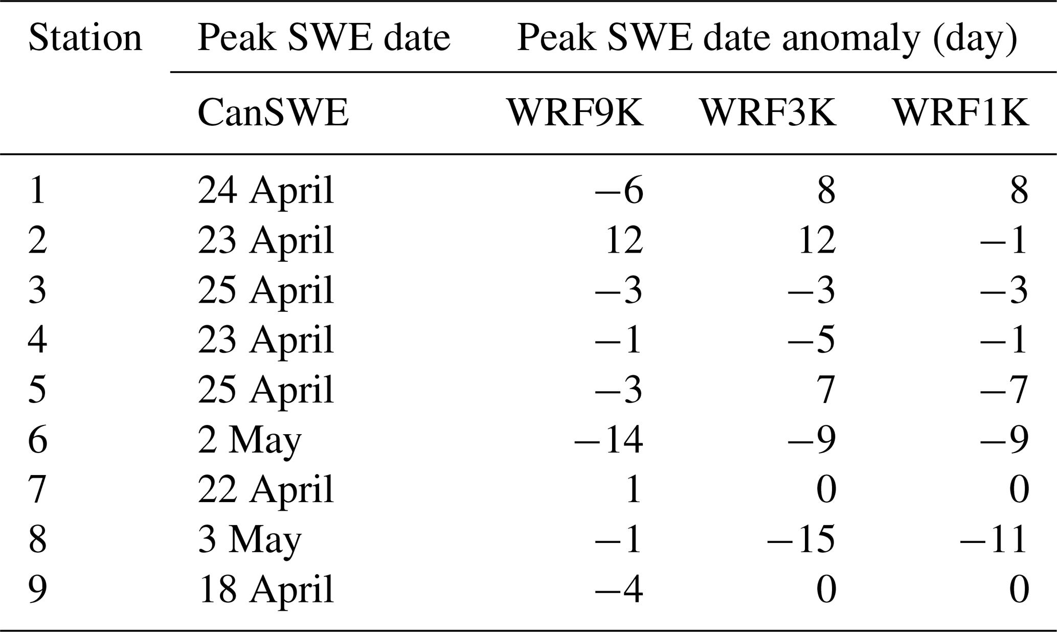
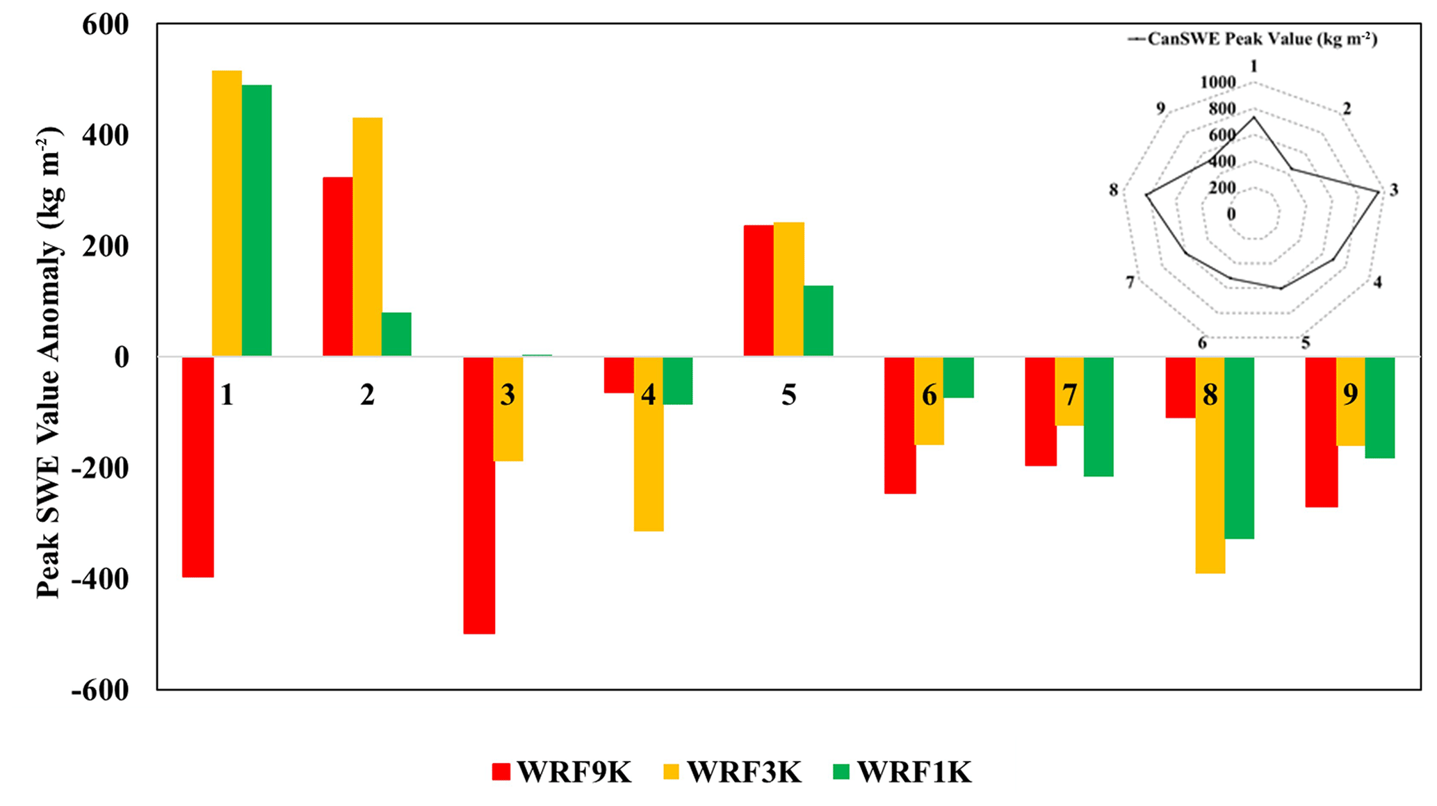
Figure 8 The anomalies in the WRF maximum SWE estimation for each station during 1 October 2017–2018. The anomaly shows how much the value of SWE is estimated more or less at each resolution (1 to 9). The value of maximum SWE for CanSWE at each station is shown in the upper right.

Although the timing of the peak SWE is quite similar across all stations, there are differences in the estimated magnitude of maximum SWE at each WRF resolution (Fig. 8). For most stations, WRF underestimates the value of the peak SWE; however, it tends to overestimate the value of the peak SWE at the two northern stations.

3.3 The role of elevation

There are clear differences in the surface terrain height imposed as the lower boundary condition for the three resolutions of WRF (Fig. 9), which suggests a possible role for elevation in the errors in simulated SWE. As is common, the spatial variability in elevation is more pronounced in the highest-resolution simulation (Fig. 9c) and becomes smoother with decreasing the spatial resolution (Fig. 9a, b). In the northern portion of the domain, where the simulated SWE estimates are less accurate, the elevation is higher and more variable than the southern areas. Because of the larger spacing of the data in WRF9K, the small-scale variability in features may not be captured. A potential explanation for the SWE biases is that WRF9K was not fine enough to resolve the localized peaks in the mountainous topography that experience a cooler mean climate and, typically, higher mean SWE.

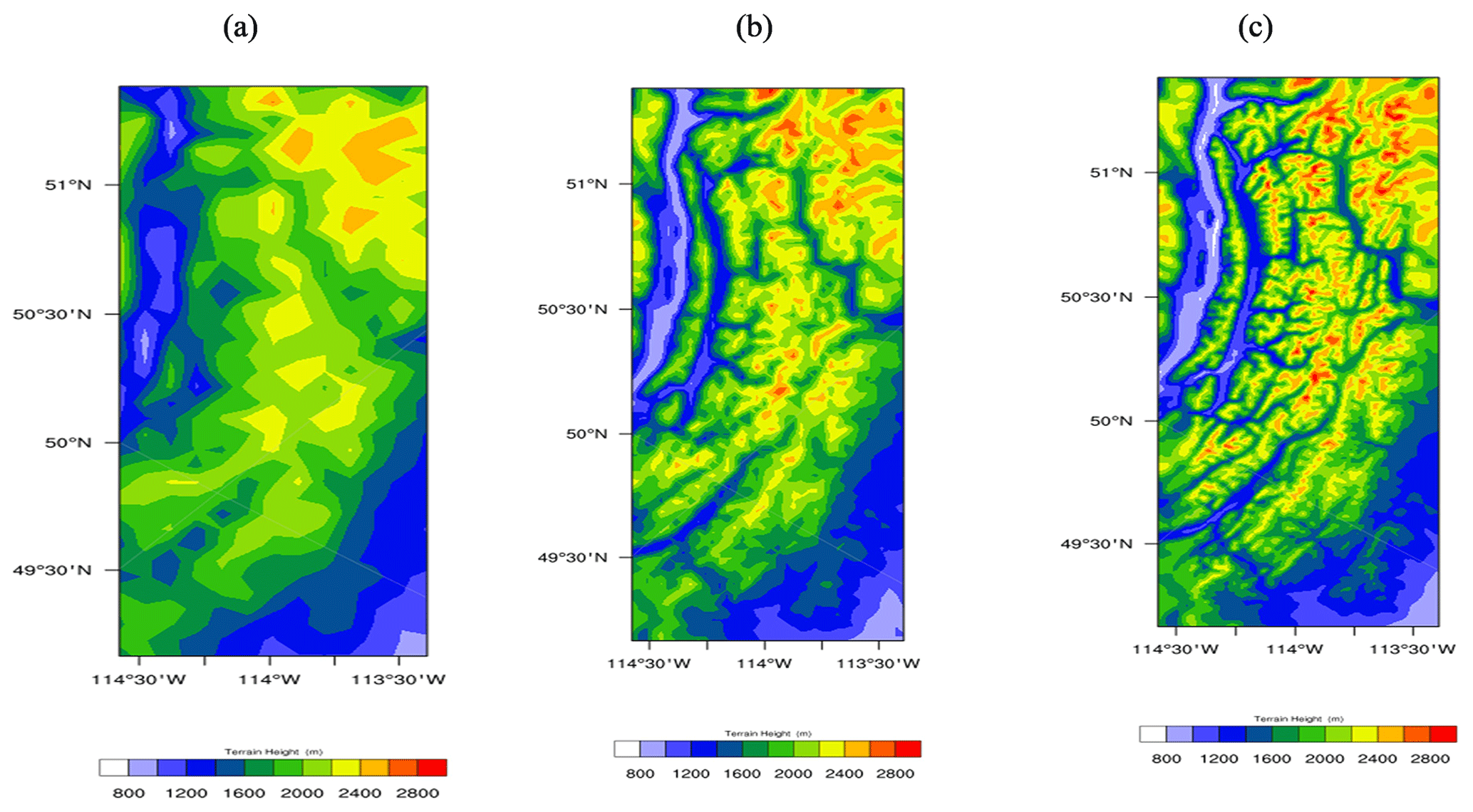
Figure 9 Spatial distribution of terrain height for WRF9K (a), WRF3K (b), and WRF1K (c) during the 2018 water year.

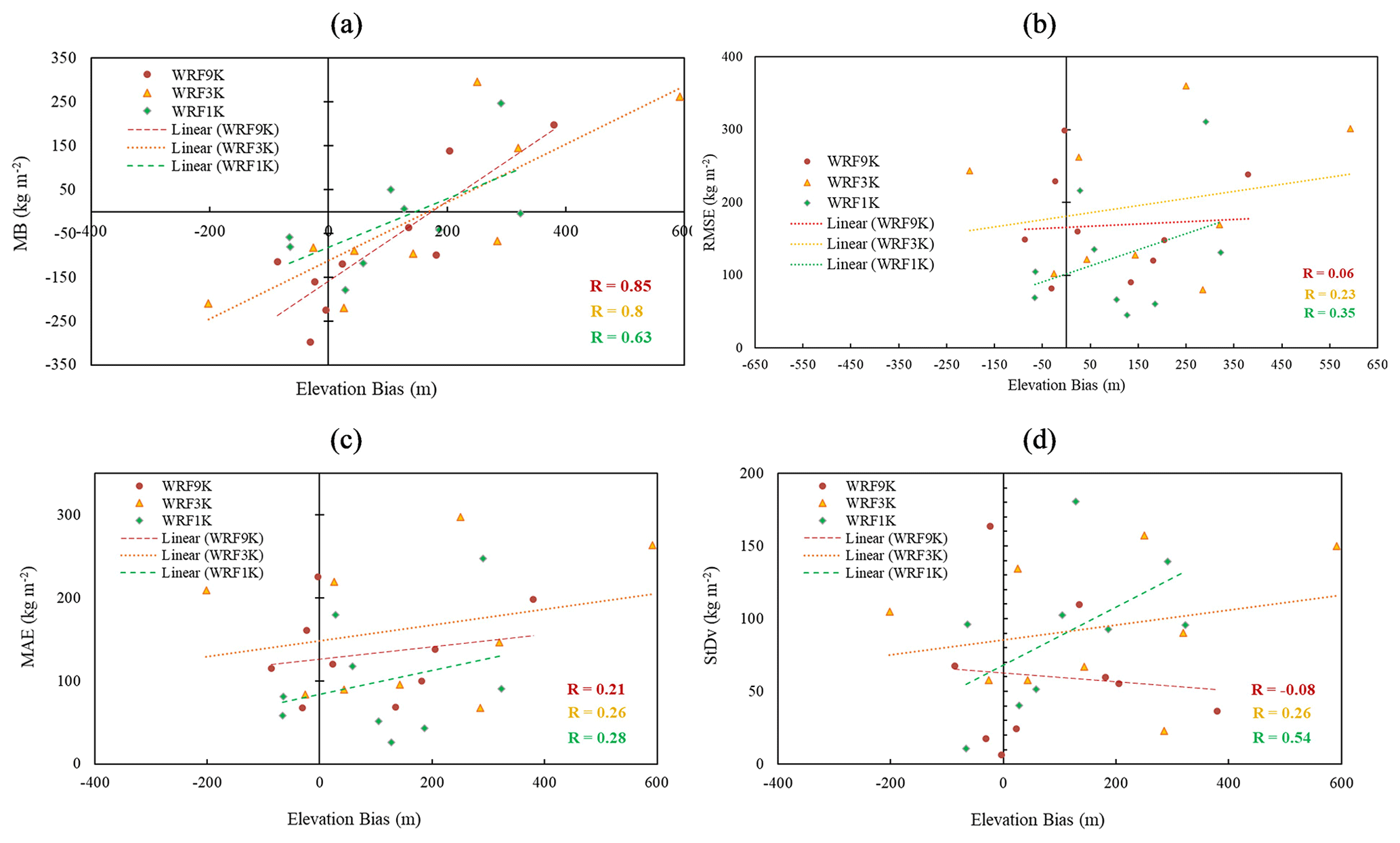
Correlation analysis shows that the absolute grid cell elevation is not correlated with SWE MB, RMSE, or MAE (not shown); however, the elevation bias – the difference between the station's actual elevation and the elevation estimated by the model in a grid cell – does appear to play a significant role. Elevation bias shows a strong positive correlation with MB at all resolutions (Fig. 10a), but an important finding is that the correlation becomes weaker at higher resolutions. In other words, when the elevation biases are large, they are a better indicator of the bias in SWE, and when elevation biases are small, they do not contribute as much to SWE errors. Therefore, it can be deduced that all WRF estimations include uncertainties and biases in simulating SWE, and one important source is biases in the grid cell elevation. On the other hand, elevation bias is not significantly correlated with the other understudied error metrics at any resolution; however, the value of the correlation coefficient becomes stronger at finer resolutions. This implies that error likely depends on atmospheric variables other than elevation. Previous research highlighted measurement inaccuracies due to instrumentation sensitivities and equipment issues like ice bridging in mountainous areas when using snow pillows (Dressler et al., 2006). Therefore, additional perspectives could be considered in future work to better understand the mechanisms and potential cause of uncertainties in SWE estimations over the mountains.

Figure 10 Elevation bias against MB (a), RMSE (b), MAE (c), and SD (d) of SWE estimation.

4 Discussion and conclusions

The objective of this study is to evaluate the potential of the high-resolution Weather Research and Forecasting (WRF) model to detect the daily values of snow water equivalent (SWE) over the South Saskatchewan River Basin (SSRB) in western Canada. Three nested domains with fine horizontal resolution of 9, 3, and 1 km are used. The Canadian historical Snow Water Equivalent (CanSWE) dataset is used to evaluate the potential of WRF to detect the spatiotemporal variability in SWE. The evaluation was conducted from 1 October 2017 to 1 October 2018, as the 2018 water year, with average SWE values during 1984 to 2021. Special focus is given to investigating the role of the WRF model grid cell size in the accurate estimation of peak SWE time and value across the watershed. Although it is acknowledged that the use of point data for the evaluation of WRF gridded SWE is problematic and introduces uncertainties because of scaling issues, we attempt to mitigate these issues by using a spatial mean taken over all stations. However, earlier studies also showed that the small-scale SWE can be representative of the grid mean value (e.g., Pan et al., 2003) for local SWE evaluation.

In general, our initial results over the averaged area show that all WRF runs behave nearly similarly and show a high value of correlation with CanSWE data, though there is a slight difference between the accumulation and melting period. All WRF estimations mainly tend to underestimate SWE over the whole year, with the largest negative bias at the coarsest resolutions. Results show that WRF fine resolution (at 3 and 1 km) significantly improves the simulations of SWE during the year over an averaged area. The coarsest run shows less accuracy during accumulation period, which is likely caused by a systematic bias in accumulated precipitation at 9 km. The underestimated precipitation over the mountainous regions at coarse resolutions has been shown by Li et al. (2019). The WRF9K model shows large errors, primarily because of its resolution limitations. At 9 km resolution, the model cannot accurately capture two key processes in mountainous areas: snow redistribution and snow deposition. These processes are especially important in mountains because snow distribution varies greatly over short distances (Mott et al., 2018; Raparelli et al., 2023). Over the whole region, there is an obvious tendency for RMSE, MB, MAE, and SD to decrease at finer resolutions, therefore decreasing the horizontal grid spacing within WRF, leading to reliable SWE estimates over the SSRB region. So, it can be concluded that the accuracy of SWE is closely related to the horizontal resolution. Earlier studies also revealed that there is a dependence of snow estimation on NWP model resolution in capturing the orographic processes over western Canada and the US (Pavelsky et al., 2011; Schirmer and Jamieson, 2015; Wrzesien et al., 2015).

The spatial variability in SWE is influenced by various processes including variability in snow accumulation that result from the preferential deposition of snow in microscale topographic depressions. Evaluation of the SWE for individual stations showed that there is less snow on the windward side of ridges and snow deposition on the leeward side. Mostly on the leeward side of the mountains, there is an underestimation of SWE for all WRF performances. There is a maximum in the SWE value in all three simulations over northern parts of the domain for both the accumulation and melting period. Low temperatures and high cyclonic activity over the northern part of the domain may cause long snow duration and high values of SWE. Local characteristics of each station, including the terrain and land cover characteristics, as well as the interactions with the local wind, would play a major role in SWE variability over the region.

Investigating the ability of the WRF model to estimate the date and the value of peak SWE for each station reveals that there is an approximately 2-week spread in the observed dates of peak SWE between late April and early May, in accordance with the observations. Although the timing of the peak SWE is quite similar across all stations, there are differences in the estimated magnitude of maximum SWE at each WRF resolution. At most stations, the value of the peak SWE is underestimated, which is consistent with the findings of previous studies (e.g., Jin and Wen, 2012; Wrzesien et al., 2018; He et al., 2019); however, WRF1K is in good agreement with CanSWE for the date and value of peak SWE. Overall, WRF can also provide reliable data for peak SWE date and value, especially at fine horizontal resolution.

Analysis of the role of elevation shows that elevation itself does not show any correlation with MB, MAE, and RMSE; however, the elevation bias shows a strong positive correlation with MB at all resolutions, which becomes weaker at higher resolutions and would be a better indicator of the bias in SWE at coarse resolution. This result highlights an important consideration when comparing point observations to output from a model grid cell, namely that the agreement in elevation between any individual station and the model's mean elevation in a grid cell will be closer, on average, for a 1 km grid cell compared to a 9 km grid cell. This is because the actual topography and associated elevation will typically be much more variable over an area of 81 km² than over 1 km². Another way to frame this is that an individual station is significantly less representative of the actual variations in elevation, precipitation, and SWE within a 9 km grid cell than a 1 km grid cell, so one might find better agreement between the model and a distributed network of stations within the grid cell. Unresolved topography contributes to the inaccurate SWE estimation at the coarse resolution. The bias in elevation, meaning the lower or upper mountains, affects the condensation of water vapor, precipitation, and topography-related temperature and therefore the amount of estimated SWE over the region. An earlier study also showed that increasing resolution in regional models resolves more small-scale features (Xu et al., 2019) and therefore improves SWE estimation. Apart from the influence of the elevation bias on MB, it does not directly affect RMSE, MAE, and SD at any resolution. Consequently, it is likely that the errors are influenced by atmospheric variables other than elevation. Therefore, additional perspectives could be considered in future work to better understand the mechanisms and potential cause of uncertainties in SWE estimations over the mountains.

To the end, this study has shown that high-resolution WRF can provide reliable and reasonable estimates of SWE values as input data for accurate hydrologic modeling, which is required for runoff forecasts. The analysis presented in this paper revealed that WRF's high resolution can represent spatiotemporal variability of SWE over the mountainous region, and it is expected to be helpful for flood forecasting in mountainous regions. However, further work is needed to remove the biases and capture the accurate value of SWE over western Canada.