Training deep learning models with a multi-station approach and static aquifer attributes for groundwater level simulation: what is the best way to leverage regionalised information?

In this study, we use deep learning models with advanced variants of recurrent neural networks, specifically long short-term memory (LSTM), gated recurrent unit (GRU), and bidirectional LSTM (BiLSTM), to simulate large-scale groundwater level (GWL) fluctuations in northern France. We develop multi-station collective training for GWL simulations, using dynamic variables (i.e. climatic) and static basin characteristics. This large-scale approach can incorporate dynamic and static features to cover more reservoir heterogeneities in the study area. Further, we investigated the performance of relevant feature extraction techniques such as clustering and wavelet transform decomposition to simplify network learning using regionalised information. Several modelling performance tests were conducted. Models specifically trained on different types of GWL, clustered based on the spectral properties, performed significantly better than models trained on the whole dataset. Clustering-based modelling reduces complexity in the training data and targets relevant information more efficiently. Applying multi-station models without prior clustering can lead the models to preferentially learn the dominant behaviour, ignoring unique local variations. In this respect, wavelet pre-processing was found to partially compensate for clustering, bringing out common temporal and spectral characteristics shared by all available GWL time series even when these characteristics are “hidden” (e.g. if their amplitude is too small). When employed along with prior clustering, using wavelet decomposition as a pre-processing technique significantly improves model performances, particularly for GWLs dominated by low-frequency interannual to decadal variations. This study advances our understanding of GWL simulation using deep learning, highlighting the importance of different model training approaches, the potential of wavelet pre-processing, and the value of incorporating static attributes.

1 Introduction

Understanding the large-scale hydrological functioning of a hydrological system is the best approach for grasping a global view of water reserves and implementing appropriate long-term management strategies (Kingston et al., 2020; Massei et al., 2020; Muñoz-Carpena et al., 2023). However, this approach typically requires constructing a large-scale hydrological model capable of capturing interactions over large areas, while respecting hydraulic continuity across the hydrological system. The model must be able to analyse and test, for example, the effects of different modes of exploitation or any other human interventions, as well as the effects of climate change over the long term. Building a large-scale model implies collecting and processing a massive database to accurately capture all the geological, oceanic, climatic, and anthropogenic forcings that drive groundwater flow. In addition, the numerical, physics-based representation of all hydrological processes occurring between the surface, sub-surface, and groundwater remains extremely complex, particularly in large-scale modelling (Paniconi and Putti, 2015). For these reasons, although progress has been made in this field, applications of physics-based models are still mainly focused on aquifers in relatively small watersheds (Massei et al., 2020; Muñoz-Carpena et al., 2023).

Under these conditions, data-driven tools have emerged as a valuable, or complements, for capturing the complex interactions across various spatio-temporal scales. These tools leverage large datasets without relying on physical representations of the non-linear processes linking climatic and hydrological signals (Hauswirth et al., 2021). Instead, they approximate these processes using simple weight matrices that replicate observed hydrological signals, whether at the scale of an aquifer or a river (Vu et al., 2023). Notably, the application of artificial intelligence (AI) algorithms, especially deep learning (DL), is expanding in hydrological sciences (Nourani et al., 2014, 2023; Rajaee et al., 2019), a trend driven by increased computational resources and the growing availability of global datasets covering hydrological and catchment attributes (Addor et al., 2017; Kratzert et al., 2023). Recent studies further highlight the potential of DL for hydrological modelling (Fang et al., 2022; Klotz et al., 2022; Kratzert et al., 2019, 2021; Nourani et al., 2021) and forecasting (Jahangir et al., 2023; Momeneh and Nourani, 2022; Jahangir and Quilty, 2023; Vu et al., 2023).

Data-driven approaches have been widely applied to rainfall-runoff modelling due to the availability of extensive runoff data. However, their application in groundwater studies is more challenging. The high cost of installing piezometers and the geological complexity of underground reservoirs, which exhibit diverse hydrodynamic behaviours across scales, make it difficult to obtain representative data. Additionally, linking groundwater data to specific locations is challenging, as aquifer delineation is more complex than catchment delineation for surface water. Groundwater systems also respond more slowly to changes, often requiring long-term data series, and are uniquely sensitive to human activities, such as pumping, which differ from influences on runoff, like river straightening or dam construction. Consequently, deep learning (DL) applications in groundwater modelling are generally limited to local scales, often using single-station data for simulation or forecasting (Chidepudi et al., 2023b; Bai and Tahmasebi, 2023; Vu et al., 2023).

In groundwater studies, the term “global models” is sometimes used to describe models trained on data from multiple wells or stations. However, this can be misleading, as it implies a broader scope than is usually intended. In the present study, we use the term “multi-station approach” to more accurately describe models that integrate data from various wells alongside external input variables. Although some studies have explored multi-station approaches for groundwater level (GWL) simulations, they are typically limited to forecasting or reconstruction using data from nearby wells. For example, Vu et al. (2021) reconstructed GWLs at single stations based on nearby station data, and Patra et al. (2023) developed “global models” focused on GWL forecasting. In another study, Gholizadeh et al. (2023) demonstrated the potential of LSTM combined with static attributes to simulate both streamflow and GWL.

Furthermore, clustering methods have shown promise in groundwater modelling, often used in hybrid models alongside AI techniques such as self-organising maps (Nourani et al., 2015, 2016; Wunsch et al., 2022b), K-means (Ahmadi et al., 2022; Kardan Moghaddam et al., 2021; Kayhomayoon et al., 2021, 2022; Nourani et al., 2023), and fuzzy C-means (Jafari et al., 2021; Nourani and Komasi, 2013; Rajaee et al., 2019; Zare and Koch, 2018). However, most of these studies focus on autoregressive approaches that depend on past GWL data. The regionalisation of GWLs through clustering and non-autoregressive DL models, which learn from comprehensive datasets with external variables, remains underexplored. Multi-station approaches that integrate both static and dynamic data or incorporate clustering have shown potential for runoff modelling (Fang et al., 2022; Hashemi et al., 2022; Klotz et al., 2022), but their utility for GWL simulations across varied hydrogeological settings requires further investigation.

To address these gaps, this study aims to provide a comprehensive evaluation of regional modelling approaches for GWL simulations compared with local models, guided by the following research questions:

• a.

  How do generalised (multi-station) models compare with specialised (single-station) models in simulating GWLs?

• b.

  Can wavelet pre-processing improve the performance of models trained on data from multiple stations across different types of GWLs?

• c.

  To what extent do static attributes or one-hot encoding techniques enhance model generalisation across varied GWL behaviours, and is their combined use more effective than individual applications? How do these models compare to those trained on stations grouped by similar spectral and temporal characteristics?

• d.

  What are the key variables influencing model learning, particularly for capturing low-frequency variability within high-frequency-dominated explanatory signals?

By investigating these questions, this study seeks to advance the understanding of regional GWL modelling and to compare multi-station and local approaches. This study focuses on “simulation” rather than “forecasting” in the context of DL applications in groundwater modelling, following the framework developed by Beven and Young (2013), where “simulation” aims to reproduce system behaviour without observed outputs, and “forecasting” predicts future states based on past observations. Our approach centres on simulating GWL dynamics to improve understanding rather than forecasting future levels. To this end, we evaluate multi-station models, incorporating static attributes and wavelet pre-processing, and compare results with local models. All experiments are conducted in a gauged setting, similar to Li et al. (2022).

The remainder of this paper is structured as follows: Sect. 2 presents the study area along with the datasets used, and Sect. 3 outlines the methodology and experimental design. Section 4 assesses the models' ability to capture variations in GWLs under different scenarios, followed by discussions on result interpretability. Section 5 presents our main conclusions and future perspectives.

2 Study area and data

The study area is approximately 80 000 km² of northern France, as depicted in Fig. 1. The available GWLs of climate-sensitive wells (i.e. not strongly affected by human activities) were obtained between 1968 and 2022 from the ADES (Accès aux Données sur les Eaux Souterraines) database (https://ades.eaufrance.fr/, last access: 8 September 2023; Winckel et al., 2022). The dataset consists of 35 mixed, 23 inertial, and 18 annual stations. All the wells considered in the study are in unconfined aquifers. In addition, the GWL data were clustered into three different types following the methodology outlined by Baulon et al. (2022b), which is based on spectral properties (i.e. characteristic timescales of variability inherent to each cluster). These clusters are identified as annual, mixed, and inertial, as depicted in Fig. 1. Specifically, the first cluster exhibits a GWL pattern predominantly influenced by the annual cycle, indicating an annual behaviour. The second cluster, the mixed, shows characteristics of both annual and interannual GWL variability. The third cluster, the inertial, is mainly characterised by its low-frequency GWL variability. In this study, low frequency refers to interannual to decadal timescales; from now in this paper, the term low frequency will be used to refer to such timescales. A comprehensive list of all analysed wells, including their identifiers, GWL types, and coordinates, is available in the Supplement (Table S1).

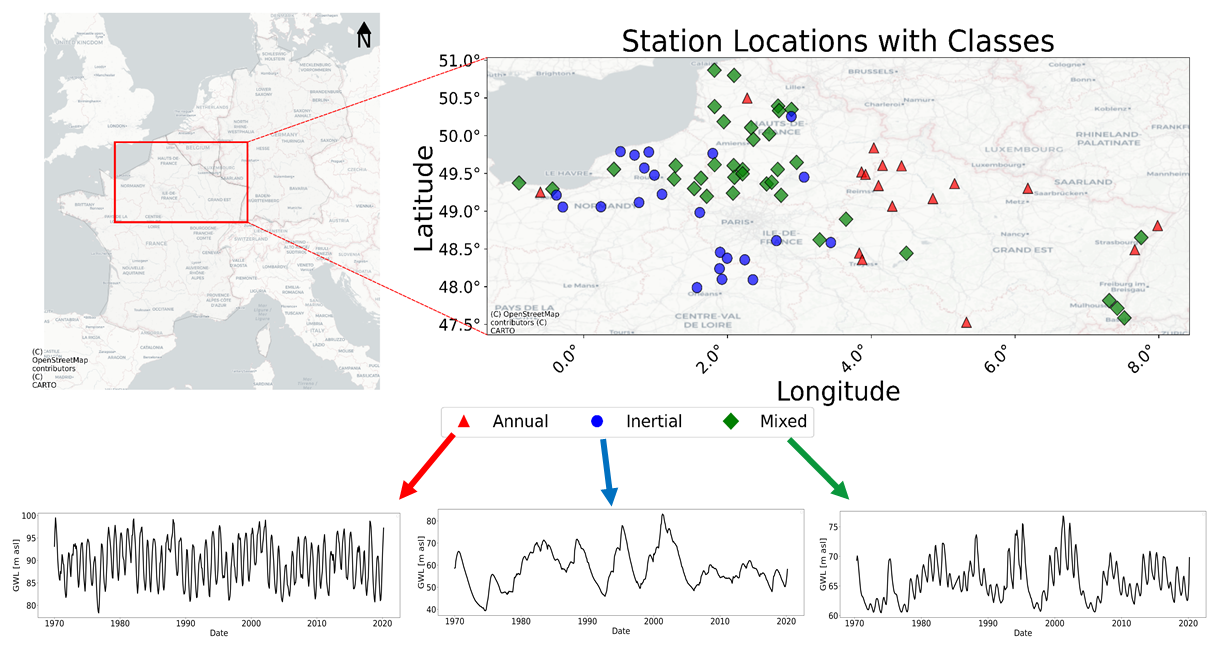
Figure 1 Clustering of GWL time series data (background layer: © OpenStreetMap contributors 2023. Distributed under the Open Data Commons Open Database License (ODbL) v1.0.) based on the spectral statistical properties (Baulon et al., 2022b): station locations (top) and representative GWL time series for each groundwater type (bottom).

We used the forcing data from ERA5, with a spatial resolution of 0.25°, to obtain the dynamic climate variables (Hersbach et al., 2020). In particular, we extract seven atmospheric variables: 10 m zonal (W–E) u-wind component (u10), 10 m meridional (S–N) v-wind component (v10), 2 m air temperature (t2m), evaporation (e), mean sea level pressure (msl), surface net solar radiation (ssr), and total precipitation (tp). These variables are among the most commonly used inputs for hydrological and land surface models, representing atmospheric conditions, circulation, moisture fluxes and radiative forcing (Kratzert et al., 2023). ERA5 is the best available global reanalysis with the data available from 1940 and is generally considered adequate for capturing regional and global hydrometeorological variations (Chidepudi et al., 2024). Addressing the uncertainty issue of ERA5 is beyond the scope of this paper and can be considered a complete research work. ERA5 Reanalysis data have uncertainty related to potential regional biases; this and their use for hydrological modelling is still ongoing research. Particularly in “large-sample hydrology”, precipitation is considered to have more bias than temperature (Clerc-Schwarzenbach et al., 2024). Nevertheless, studies conducted recently concluded that ERA5 temperature and precipitation biases had been consistently reduced compared to ERA-Interim and were found to be quite accurate for hydrological modelling, for instance, in the case of the conterminous US (Tarek et al., 2020). Gualtieri (2022) highlighted that ERA5 uncertainties are greatest in mountainous and coastal locations (in the study presented herein, only 1 station out of 76 is located within the 10–15 km from the coast). Finally, one recent study concluded that the use of ERA5 precipitation was recommended for all extra-tropical regions (Lavers et al., 2022). Nevertheless, we evaluated different alternative reanalysis products, such as the SAFRAN (Système d'Analyse Fournissant des Renseignements Atmosphériques à la Neige) reanalysis developed specifically for France (Vidal et al., 2010). ERA5 and SAFRAN precipitation appeared to have the same low-frequency timescales of variability as our GWL time series, as displayed in Fig. 3 (this paper) and in Fig. 11 in Chidepudi et al. (2023b). ERA 5, then, is suitable for our purpose.

Table 1 Summary of the static attributes used in the current study. A comprehensive explanation of all descriptions can be found at the URLs provided in the third column.

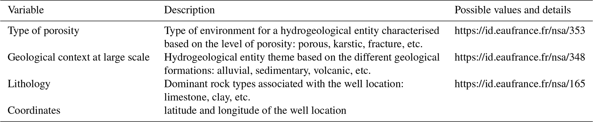
All links in this table were accessed on 19 July 2023.

Figure 2 Distribution of geological features by class.

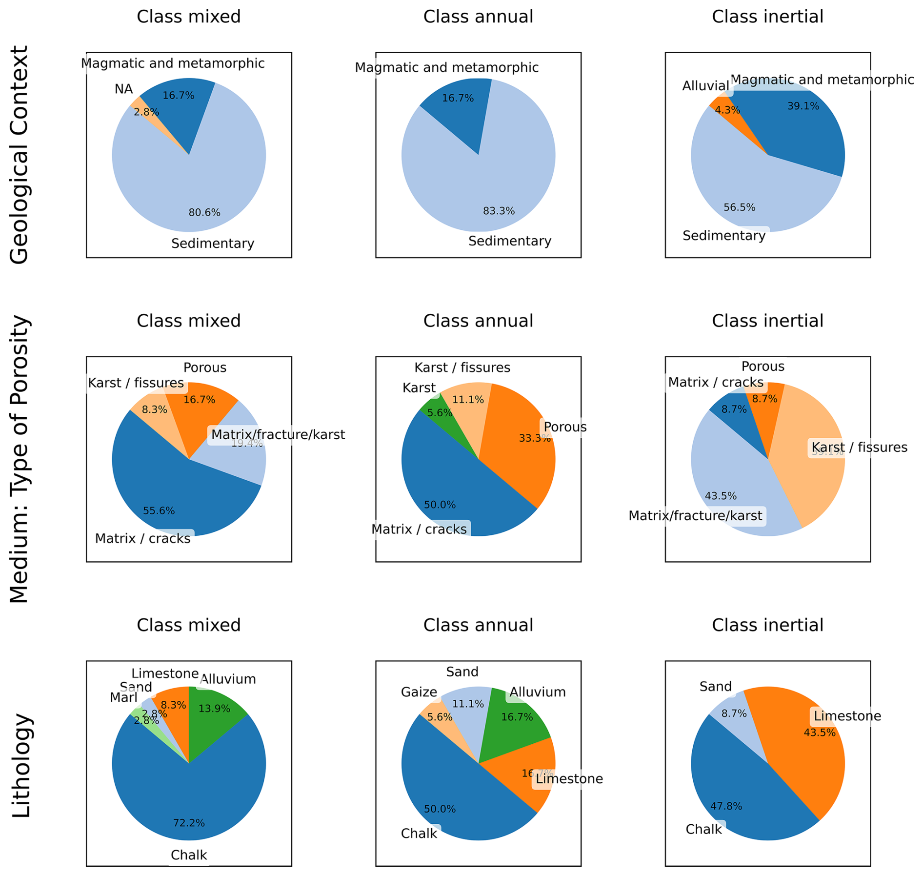
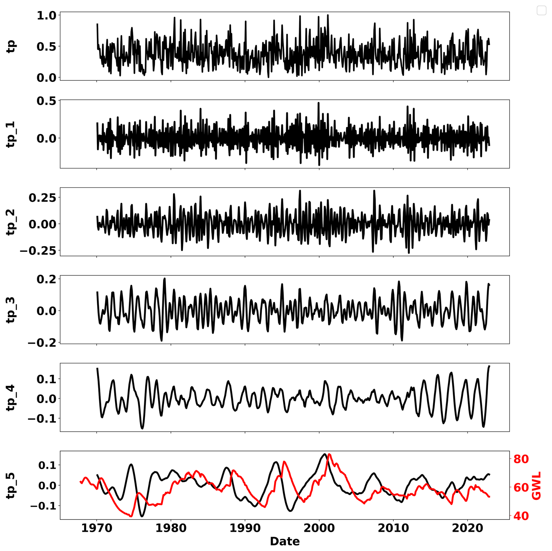
Figure 3 Total precipitation (tp) and its wavelet components: high (tp_1) to low frequency (tp_5) and GWL (in red).

In this work, we also included static attributes (Table 1 and Fig. 2) to assess whether such informative data would help to better represent small differences between GWL time series owing to different contexts (e.g. type of porosity, overall geological context, lithology, location). Static attributes are available for different ranges of aquifer classes with different resolutions. We took the static attribute's value corresponding to each well's location. Static attributes were extracted from the BDLISA (Base de Donnée des Limites des Systèmes Aquifères) (https://bdlisa.eaufrance.fr/, last access: 19 July 2023) database, which provides point-scale information. BDLISA is based on a mix of information from geological maps, piezometric maps, and hydrochemistry at a scale of 25 km. For our study, we kept information coming from BDLISA at its original scale (25 km), which means aquifer static attributes have a resolution of 25 km. This information from BDLISA should be understood as a local–regional description of aquifers. Exact details of static attributes for each GWL station can be found in Table S1.

The decision to include the relevant static attributes comes from a trade-off between the transposability of models and the availability of attributes, as we need to ensure that all those variables are widely available at the required resolution. For instance, hydraulic conductivity might not be easily available everywhere, and high spatial heterogeneity that would not be accounted for owing to available spatial resolution may lead to inconsistent results (a 25 km resolution might not be relevant when aquifers are highly heterogeneous). Exploring the role of static attributes in more detail would require much further work than what was conducted in this study.

3 Methodology: from single-station to multi-station training

3.1 Theoretical modelling background

In the present study, we explored the use of recurrent-based deep learning models to simulate GWLs across multiple stations using different approaches as described in Sect. 3.2. We apply three types of recurrent neural networks: long short-term memory (LSTM; Hochreiter and Schmidhuber, 1997), gated recurrent unit (GRU; Cho et al., 2014), and bidirectional LSTM (BiLSTM; Graves and Schmidhuber, 2005), alongside a wavelet pre-processing strategy (BC-MODWT). Each of these methods is designed to process data that changes over time, capturing patterns and dependencies that occur over extended periods. In brief, LSTM has a single memory cell and three gates (forget, input, and output) to manage the flow of information. GRU simplifies this design, with only two gates (reset and update), to increase computational efficiency by reducing the number of parameters compared to LSTM. BiLSTM further optimises data analysis by simultaneously processing sequences in both forward and backward directions. These models are particularly good at identifying various patterns in data sequences, making them ideal for simulating GWLs that change over time (Vu et al., 2023).

We also explored the potential of wavelet decomposition (BC-MODWT) to decompose the data into components of varying frequencies (Fig. 3), from high to low, to provide more detailed input to the DL models to better simulate the GWLs. As explained in Chidepudi et al. (2023b), decomposition depth (i.e. the choice of the number of components) was constrained by the trade-off between (1) achieving a sufficient high level of decomposition to ensure the low-frequency variability is properly reached and (2) keeping the number of coefficients affected by boundary conditions as low as possible since these have to be ultimately removed from the input time series. All input time series were decomposed using BC-MODWT, with a decomposition depth of 4 as in Chidepudi et al. (2023b). Figure 3 illustrates the decomposition result for the precipitation time series. A four-level decomposition efficiently extracted the first four so-called wavelet details (tp_1 to tp_4), while the last fifth (so-called smooth) tp_5 component remains of sufficiently low frequency. It is visible that tp_5, almost invisible in the original tp precipitation time series, corresponds well to the variability of the most inertial GWL types (Fig. 3, in red, with a few months' time lag with respect to tp).

3.1.1 Model training and evaluation

To maintain consistent comparison criteria across all methods evaluated in the study, Bayesian optimisation was used for hyperparameter tuning. Details of the range of hyperparameters used are shown in Table 2. Furthermore, the range of hyperparameters used for optimisation was standardised across all methods, following the best practices outlined for both standalone and wavelet-assisted models, as detailed in Chidepudi et al. (2023b) and Quilty and Adamowski (2018).

Table 2 Hyperparameter details (modified and adapted from Chidepudi et al., 2023b).

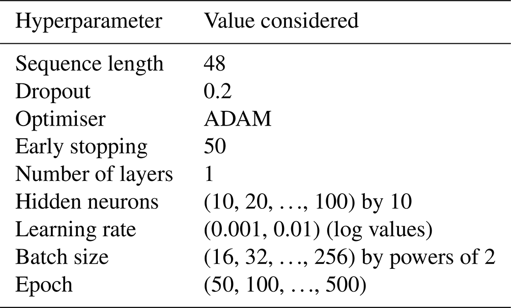
Figure 4 Comparison of performance of single-layer DL models (a, c, e) and multiple-layer DL models (b, d, f) with respect to single-station models as a reference. SA represents standalone models, while Wav represents wavelet-assisted models.

However, we made an important update to the model architecture by setting the number of layers to one for all models, rather than optimising it. This decision was based on findings from Fig. 4, which suggested that optimising the number of layers did not significantly improve performance, in line with recent studies in related fields like rainfall-runoff modelling (Kratzert et al., 2019, 2021). Other adjustments included reducing the number of initialisations to 10 and setting the number of trials in the Bayesian optimisation to 30. These changes were aimed at reducing the computational requirements of our approach, making it more efficient without significantly affecting the quality of our results, and are consistent with recent studies (Wunsch et al., 2022a).

The intricacies and specific technical details of the architectures of these models are well documented in the existing body of deep learning research applied to hydrological simulations, as detailed in several studies (Chidepudi et al., 2023b, 2024; Fang et al., 2022; Kratzert et al., 2021; Li et al., 2022; Vu et al., 2023).

To further interpret and decrypt the results, we used the SHAP or Shapley Additive Explanations approach (Lundberg and Lee, 2017), which is an increasingly popular game-centric approach for explaining the outcomes of deep learning models. SHAP explains how each input feature influences the model's simulations. It does this by highlighting two key aspects: the importance of each variable, where a higher mean absolute SHAP value indicates a greater impact, and the nature of that impact, whether positive or negative.

3.2 Experimental design

This section details the experimental design used to assess the effectiveness of training models using data from all available stations. Our study uses different strategies to incorporate numerical and categorical data into the models. The aim is to improve the accuracy of GWL simulations by exploring ways of incorporating regional variability into the models. The experimental setup is structured to test different modelling strategies, as described below and visualised in Figs. 5 and 6.

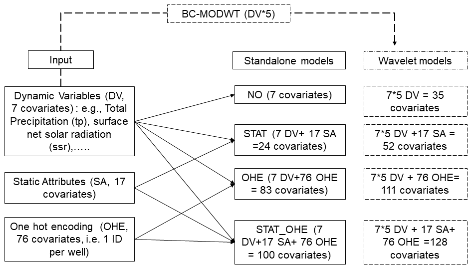
Figure 5 Construction of the different multi-station approaches for standalone and wavelet models and associated covariates (input features).

Figure 6 Comparison of different approaches adopted in the current study: single station (top), multi-station without clustering (middle), and multi-station with clustering based on spectral properties (bottom). (Background layer: © OpenStreetMap contributors 2023. Distributed under the Open Data Commons Open Database License (ODbL) v1.0.)

1. Single-station or local models (models trained and tested individually per station). These models are trained and evaluated on data from individual stations. As a baseline, their performance provides a benchmark for evaluating the effectiveness of more generalised models. This approach is dominant in developing data-driven models for GWL simulations and is discussed in detail in Chidepudi et al. (2023b, 2024). The optimal hyperparameters for all standalone and wavelet models in the single-station approach are presented in Tables S3 and S4.

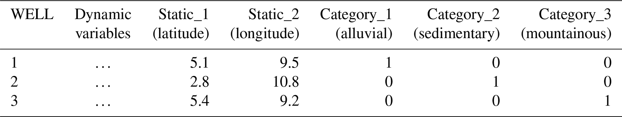
2. Multi-station models (models trained and tested together on many stations). These models are trained using data aggregated from multiple stations and tested with different input configurations. In the first configuration (NO), models are trained on all stations using dynamic variables only, excluding static attributes and one-hot encoding. In the second configuration (OHE), models are trained using one-hot encoding to represent individual station ID information as binary vectors to ensure that the specific information is obtained from collective training. Li et al. (2022) also showed that one-hot vector (one-hot encoding using basin ID) could produce similar results to using catchment attributes in gauged basin scenarios. One-hot encoding serves as an alternative to incorporating static attributes directly into the model (Table 3). In the third configuration (STAT: static attributes and dynamic variables), models include both static attributes (e.g. latitude, longitude) and dynamic variables as inputs, with categorical variables encoded similarly to one-hot encoding but represented in separate columns for each unique value or class (Table 4). In the fourth configuration (STAT_OHE), we combine static attributes, one-hot encoding for well IDs, and dynamic variables to provide a comprehensive dataset for model training. In other words, it is a combination of the two input strategies above. The covariates and input shapes for various multi-station approaches are summarised in Fig. 5, and the exact shapes of 3D tensors are provided in Table S5.

Table 3 Example of one-hot encoding based on different wells. The ellipses denote the usual time series data of dynamic variables.

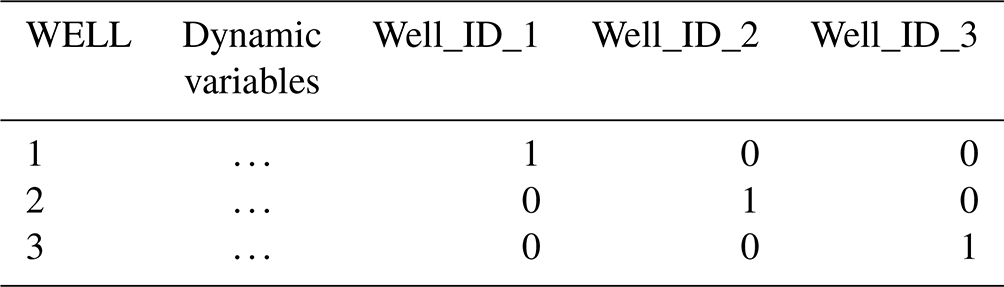
Table 4 Example with static attributes of numeric and categorical types.

In addition to these configurations, we investigated the performance of multi-station models trained on GWLs with similar spectral statistical properties. This approach assesses the effectiveness of models tailored to specific GWL behaviours compared to more generalised models using the aforementioned strategies. For validation purposes, in this study, the Kling–Gupta efficiency (KGE; Gupta et al., 2009) is preferred over the Nash–Sutcliffe efficiency (NSE) and other metrics because it offers a more comprehensive evaluation by integrating three aspects of model error: correlation, bias, and the ratio of standard deviations.

For the single-station approach, the data were split into training (80 %) and testing sets (20 %) as described in Chidepudi et al. (2023b). Furthermore, to facilitate hyperparameter tuning, the last 20 % of the training data were used as a validation set. For the multi-station approach, the train–test split was also performed at each station, following the same procedure as the single-station approach. However, the data from all stations were then collectively combined during the training. The rationale behind the specific train–test split is to ensure that the models capture the multi-annual to decadal variability in observed GWLs. To achieve this, data spanning a minimum of 34 years (1970–2014) were used for training, while data spanning the most recent 8.66 years (January 2015–August 2023) were reserved for testing. The testing period was chosen to be the most recent years, allowing for an evaluation of the model's performance on the latest available data. The specific dates and periods used for training and testing at each station are detailed in Table S2.

Our methodology for comparing single-station and multi-station approaches, both with and without prior clustering based on spectral properties, is consistent with the research conducted in rainfall-runoff modelling by Hashemi et al. (2022), where the catchments were divided into five subsets according to hydrological regimes. This comprehensive experimental design aims to identify the most effective strategies for using multi-station data in the simulation of groundwater level variations. Detailed hyperparameters for all the multi-station standalone and wavelet models can be found in Tables S6–S9.

4 Capabilities, performances, and interpretability of multi-station approaches

4.1 Different strategies for multi-station approach

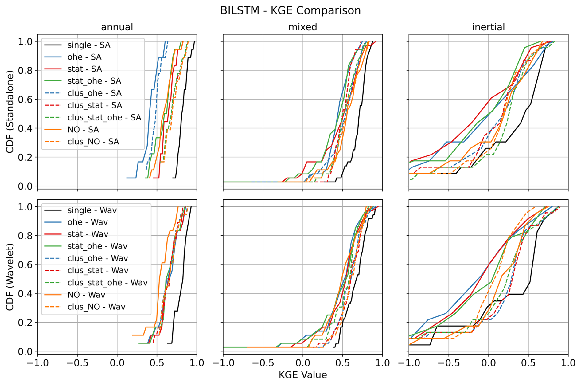
All models tested in the case of this study performed more or less equivalently and eventually yielded very satisfactory results. This can be attested by the performance comparison shown in Fig. 4 (comparison of the three model types in single-station mode) and by comparing Fig. 7 (GRU multi-station) with Figs. A1 (LSTM multi-station) and A2 (BiLSTM multi-station). We finally decided to favour the GRU architecture, owing to its recognised computational efficiency over more traditional LSTM-based architectures (Cho et al., 2014; Cai et al., 2021; Chidepudi et al., 2023b, 2024)

Figure 7 CDF comparison of KGE values of the GRU with different approaches and GWL types.

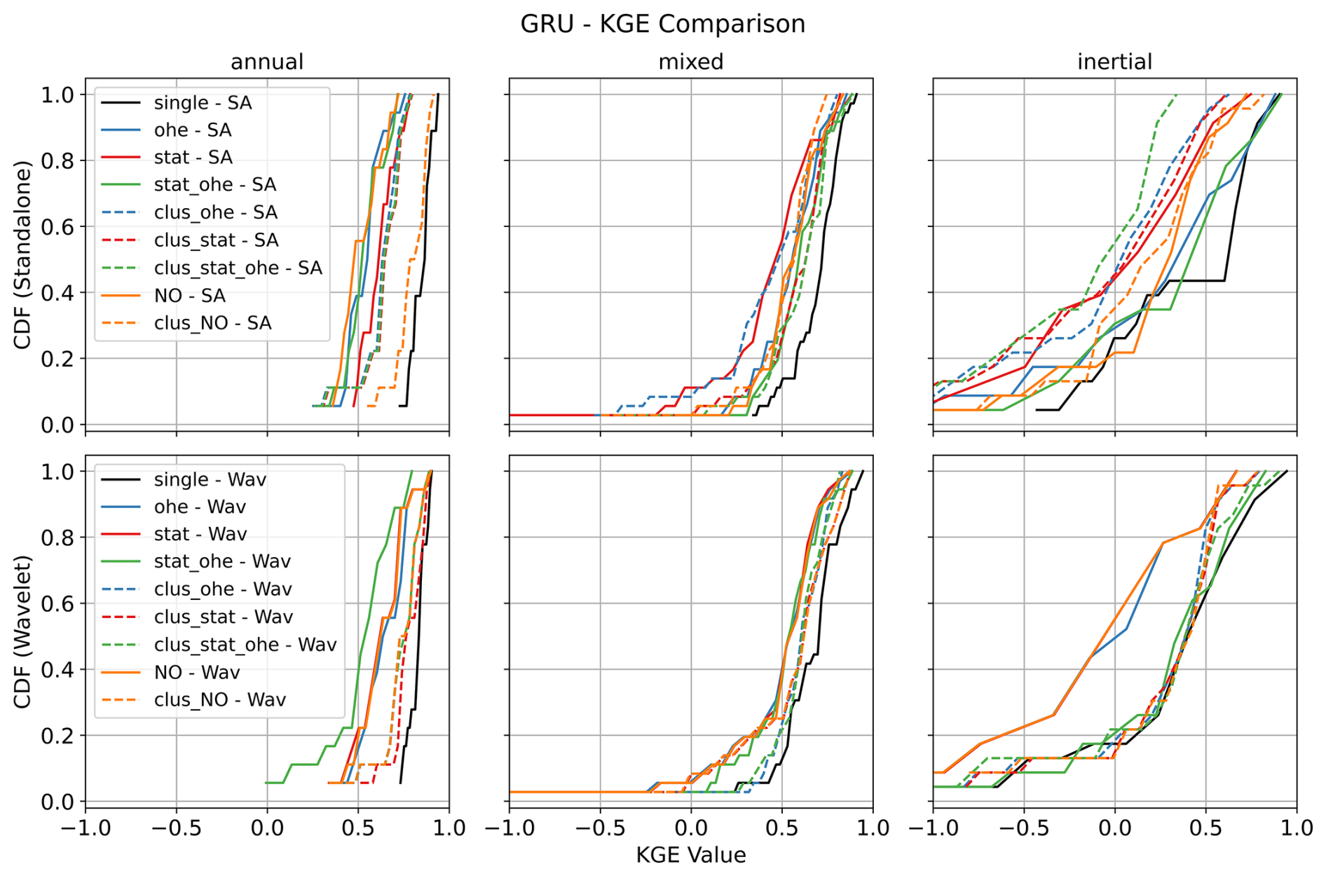
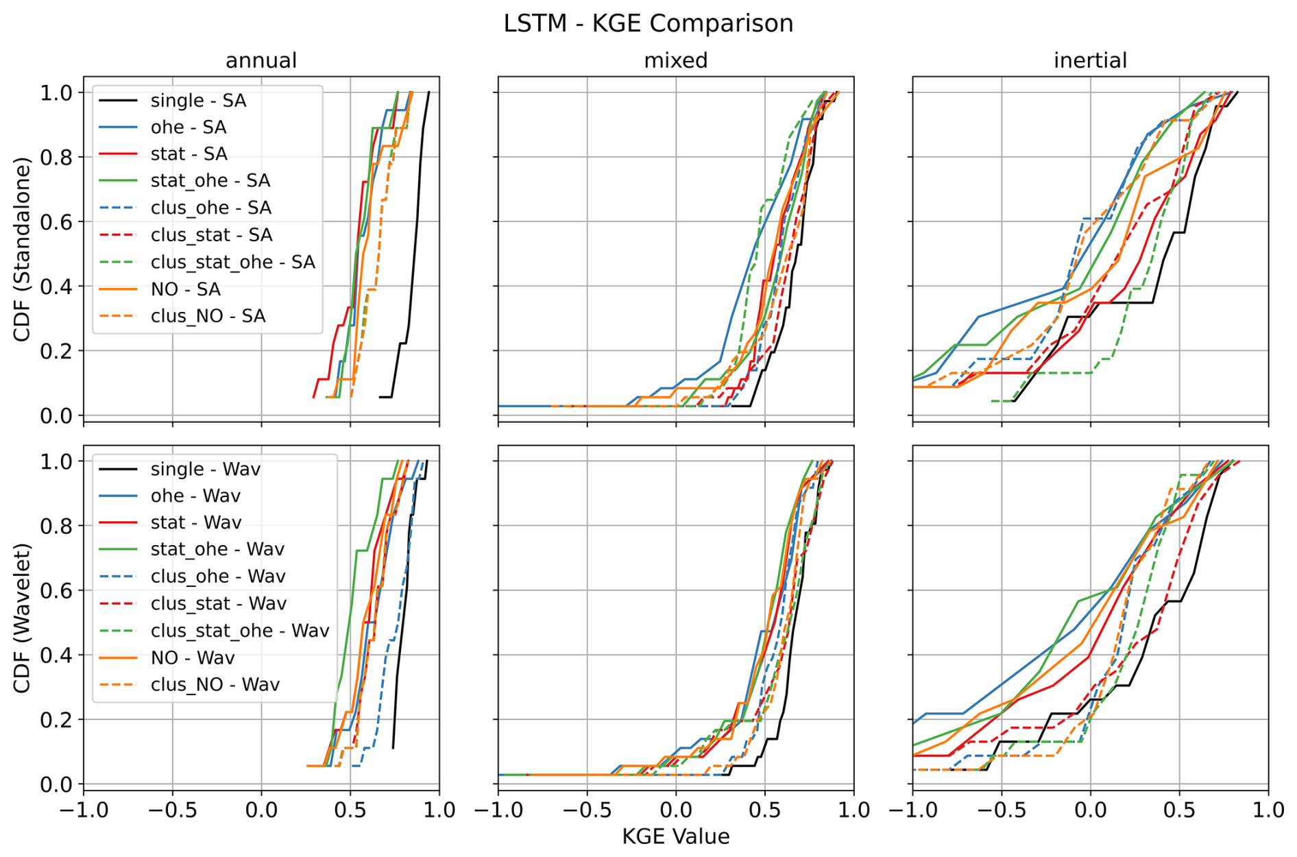
Figure 7 shows the results of different GRU model configurations for simulating GWLs. The first row shows the performance of the standalone GRU model for different GWL categories, while the second row shows the wavelet-assisted GRU results.

Several observations can be made from Fig. 7. Wavelet pre-processing generally improves model performance, especially in the inertial GWL category, where cumulative distribution functions (CDFs) are steeper and shifted to the right, indicating a higher proportion of simulations with high performance. This is in line with previous findings as already reported in our previous works (Chidepudi et al., 2023a, 2024). This demonstrates the wavelet decomposition ability to extract “hidden” inertial dynamics features which facilitate their assimilation by the model in the learning process. In other words, the improvement attributed to wavelet pre-processing becomes more pronounced as we move from annual to mixed and then further to inertial behaviour. This is because in the case of annual-type GWL, the dominant variability (annual cycle) is already well expressed in several input variables (e.g. t2m, msl, ssr). In the case of mixed- and inertial GWL types, the dominant low-frequency variability, while also present, is barely expressed, almost “hidden”, in the input data and becomes prominent in GWL due to the low-pass filtering action of aquifers (Baulon et al., 2022a; Schuite et al., 2019). Wavelet decomposition allows the unravelling of such hidden information, helping the neural networks to reach it for enhanced learning. This is illustrated in Fig. 3 with the low-frequency component of precipitation (tp5) matching the variations of one inertial-type GWL (in red, with a few months' lag time), whereas it is masked by other higher-frequency components in the original precipitation time series (tp). The combination of static attributes and OHE gives competitive results, particularly in the inertial category, demonstrating the effectiveness of this method without the need for prior clustering of GWL behaviour. Multi-station models, when trained separately for each GWL cluster, generally outperform those trained on aggregated data. This is reflected in higher KGE values for cluster-specific models, suggesting a better representation of the unique characteristics of each GWL type. However, this advantage diminishes for mixed GWLs, which are the majority in the study area. Although single-station models perform best for all GWL types, some multi-station models approach or match their performance, highlighting their potential for regional-scale GWL simulations. For the annual GWL category, models trained on mixed GWL data without wavelet pre-processing and relying solely on static attributes do not show significant performance improvements, suggesting that static features alone may not adequately represent the dynamic nature of groundwater behaviour.

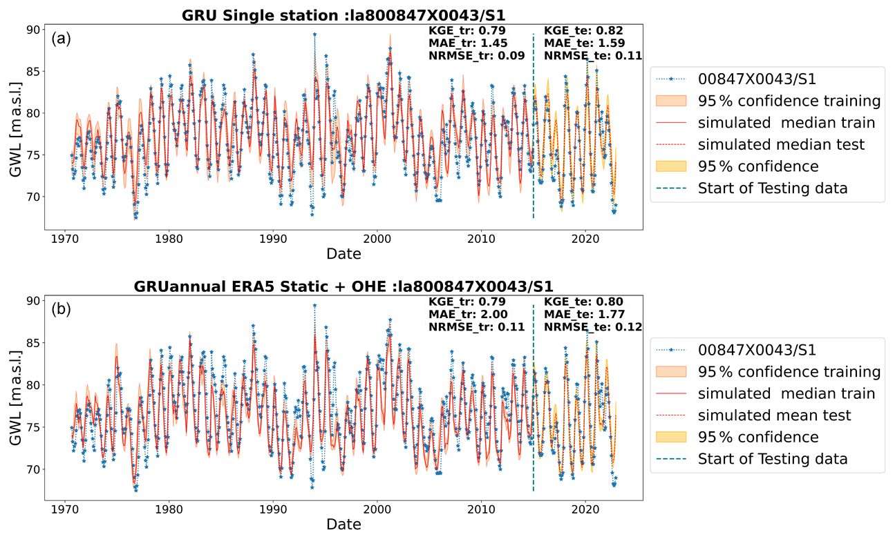
Figure 8 Results with wavelet-assisted GRU in the annual type of GWLs through (a) single-station and (b) multi-station models trained on the annual type of GWLs with static attributes and OHE.

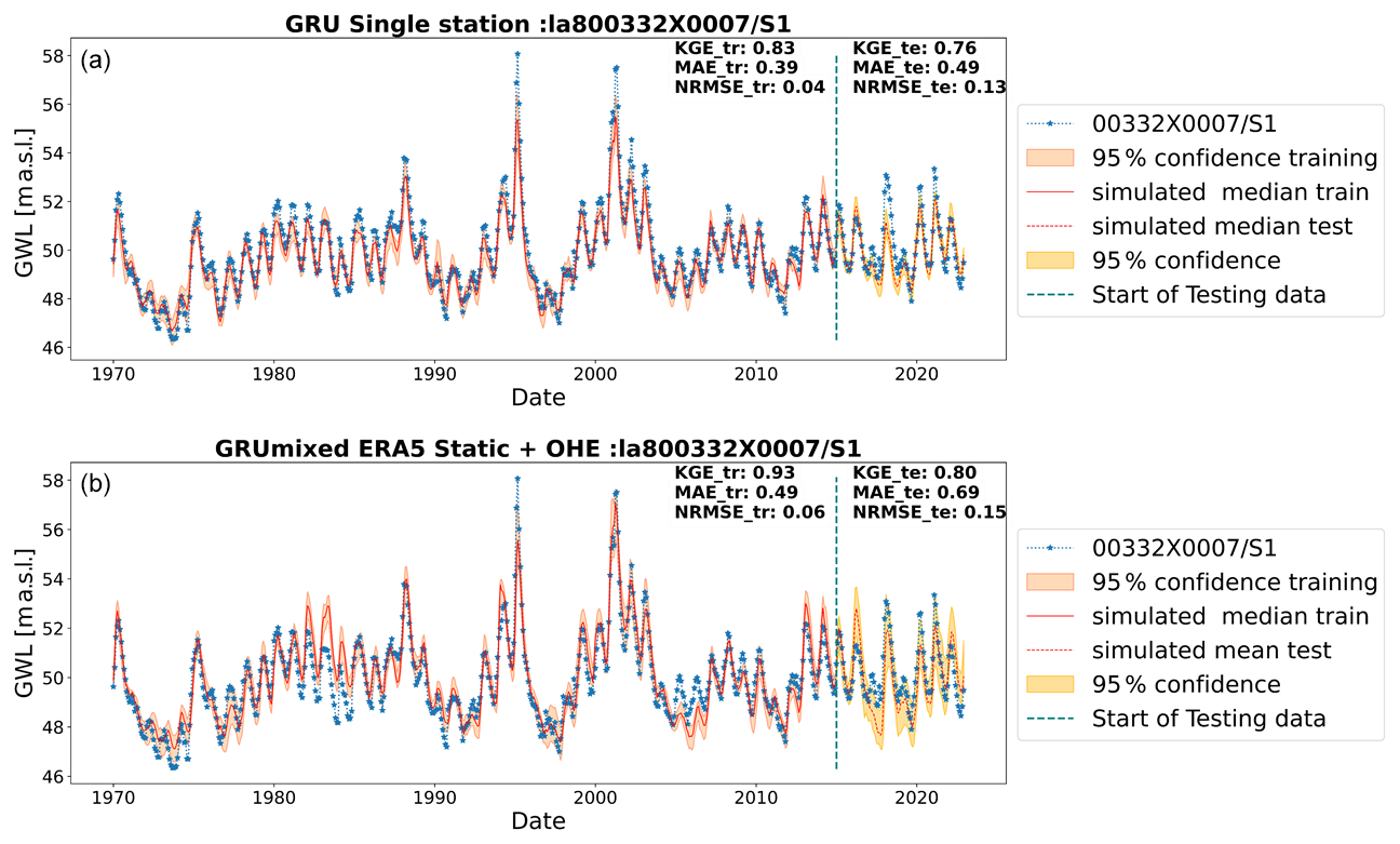
Figure 9 Results with wavelet-assisted GRU in the mixed type of GWLs through (a) single-station and (b) multi-station models trained on the mixed type of GWLs with static attributes and OHE.

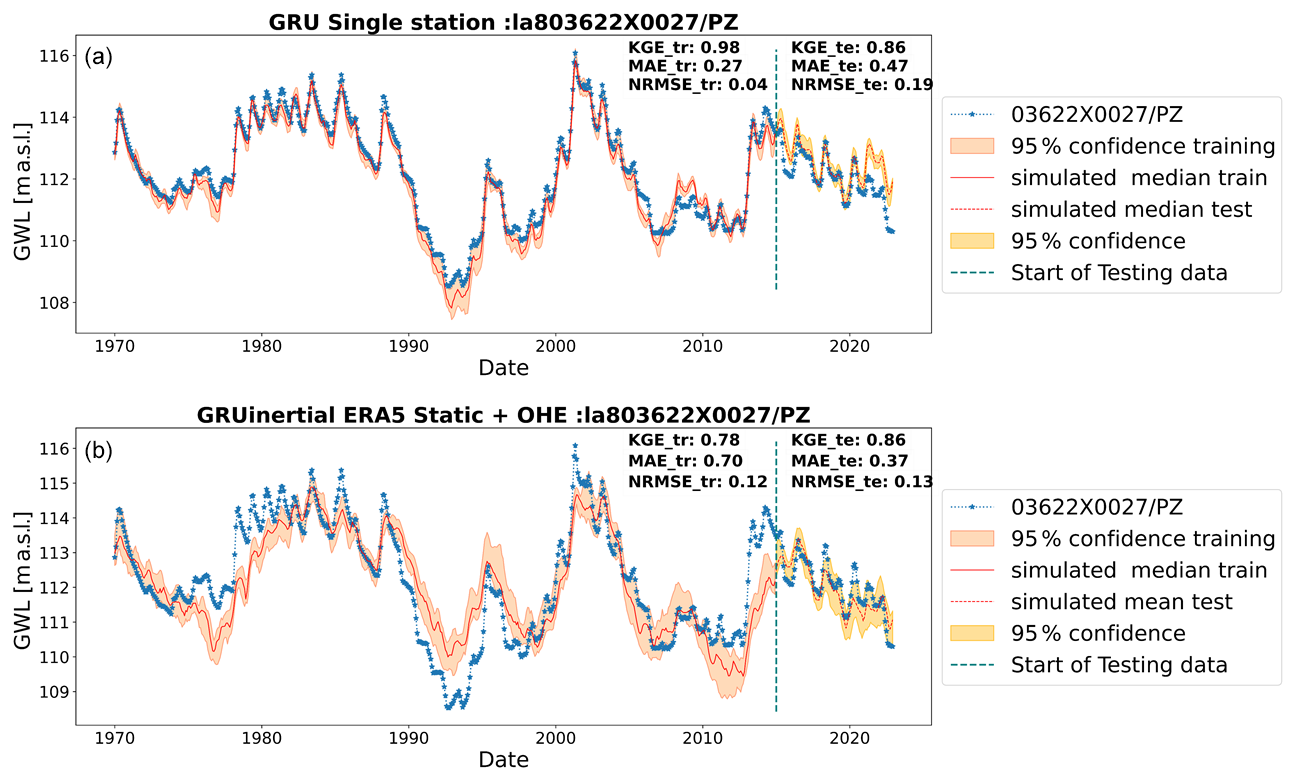
Figure 10 Results with wavelet-assisted GRU in the inertial type of GWLs through (a) single-station and (b) multi-station models trained inertial type of GWLs with static attributes and OHE.

Figures 8–10 show the best GWL simulations obtained of different types (annual, mixed, and inertial) for single and multi-station models. For those particular cases, both approaches perform similarly and lead to good performance. However, the single-station modelling seems to perform best for inertial GWL type for training by simple visual assessment, and it is clear from the comparison of KGE values of all stations (Fig. 7) that the more specialised single-station models generally gave the best results overall, although not significantly. This is more specifically true for inertial GWL, where regional model performances reach the same level as single-station models. While single-station models perform well, multi-station models are valuable when single-station modelling is impractical due to data limitations or computational requirements. For instance, for inertial types where the length of training data might be an issue (e.g. Chidepudi et al., 2024), the performance of the wavelet multi-station models was completely comparable to single-station models (Fig. 7, wavelet models/inertial types), showing that in the case of data limitation, the regional approach seems to compensate for the lack of temporal depth of available time series.

In summary, wavelet-assisted GRU models are particularly effective, especially for low-frequency dominated GWL behaviour, and multi-station models designed for specific GWL types (i.e. training over specific pre-clustered datasets) generally outperform generalised models. The multi-station approach is sensitive to the dominant GWL type in the training dataset, with the best results identified in models trained for the predominant mixed GWL type. To address the issue of models learning dominant behaviour in the collective training of multi-station approaches, future investigations may involve generating synthetic time series with randomised amplitude changes of constituting frequencies to increase the dataset while balancing all the important behaviours. This could also help in understanding the influence of the size of the dataset on using multi-station approaches.

4.2 Understanding GWL simulations through SHAP interpretability

This section deals with a deeper understanding of the simulations from the insights obtained from the SHAP analysis on the model's interpretability. Here, we investigated the key contributing factors for GWL simulations in different approaches that were previously evaluated above in terms of accuracy.

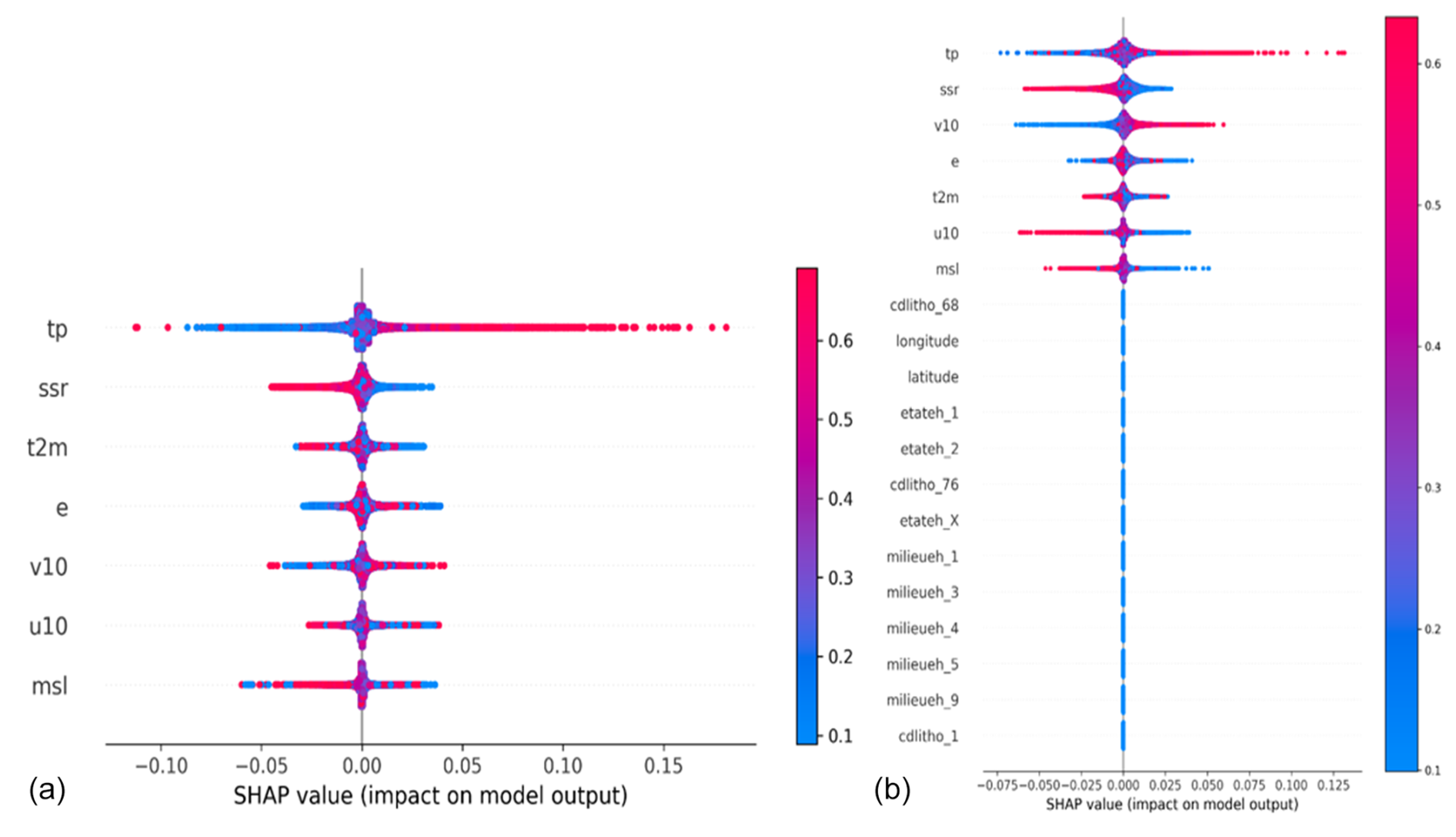
Figure 11 SHAP summary plot examples for single-station models (a) and multi-station models with static attributes (b). The colour bar shows the range of feature values, with red depicting larger values and blue referring to smaller ones.

Figure 11a shows the SHAP representative summary plot for the standalone models using a single-station approach. These plots highlight the influence of different variables/attributes on the final simulation. In particular, the distribution of data points on the SHAP diagram indicates either a positive (right side on the x axis) or negative (left side on the x axis) impact on the output variable. In contrast, the colour scale indicates the range of feature values in which red represents large values, and blue represents small ones of the corresponding feature. Features (input variables) are organised from the most to the least influencing, from top to bottom, based on each feature's mean absolute SHAP values. For instance, in Fig. 11a, total precipitation (tp) is the most influencing feature on the GWL output, and the large feature values on the right (red) correspond to a positive influence on GWL (high GWL with high total precipitation). On the left side, negative tp SHAP values indicate lower precipitation values contributing to the low GWLs.

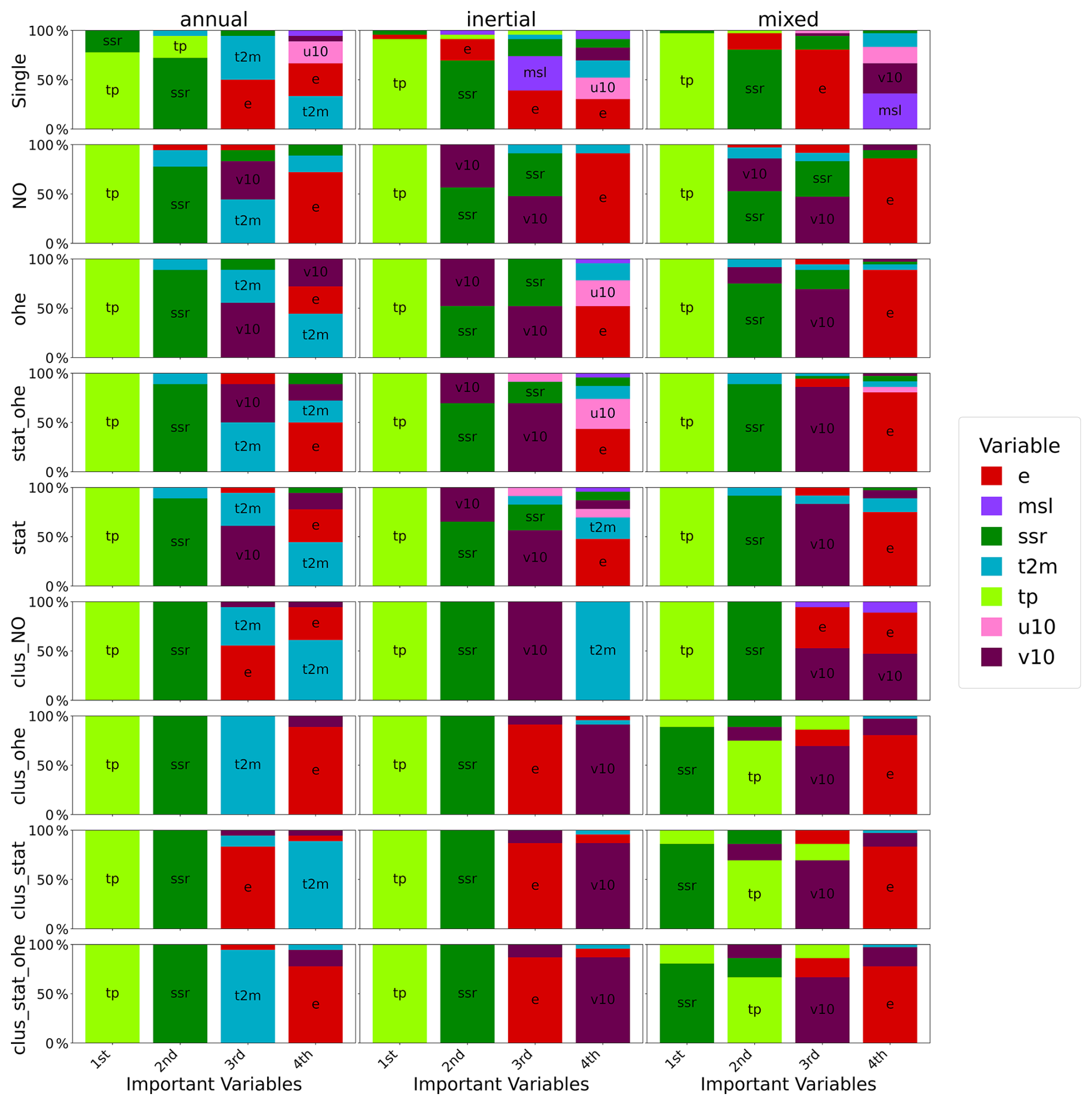
Figure 12 Top four important variables by cluster for standalone GRU models with different approaches. On the y axis, percentage of stations for each variable within the cluster.

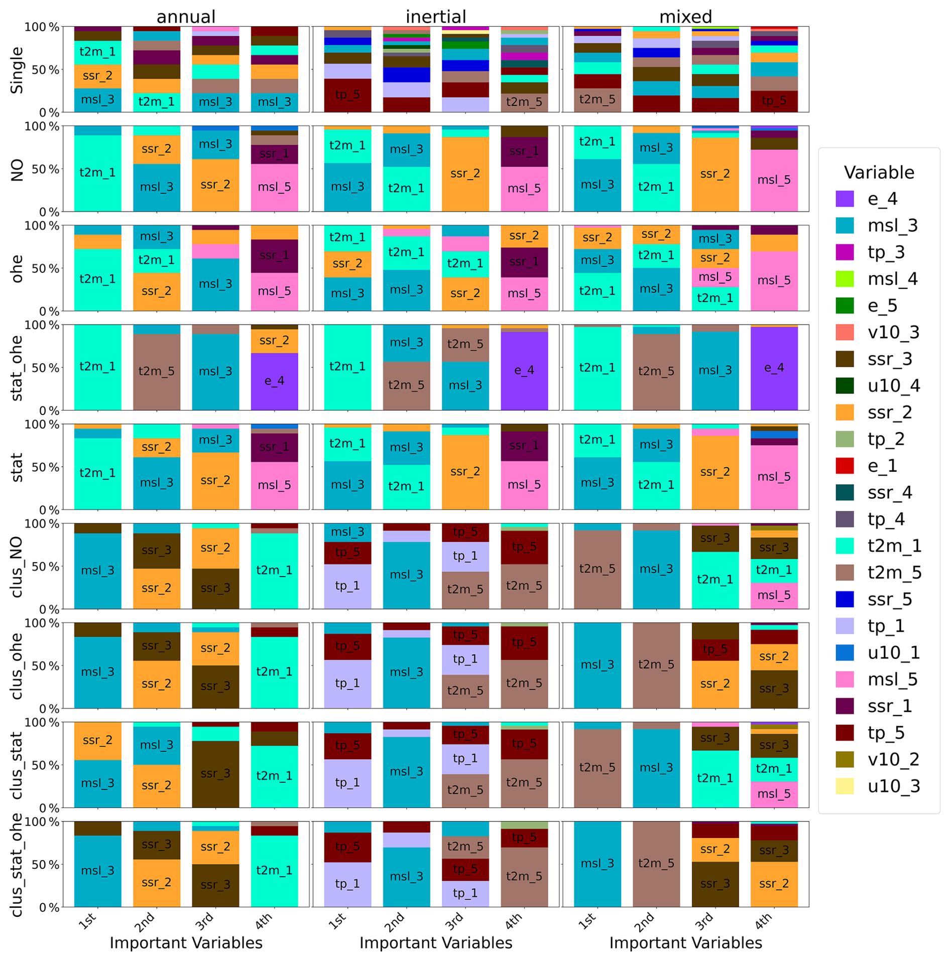
Figure 13 Top four important variables in regional GRU wavelet-assisted models trained with different approaches for different classes: wavelet components of each variable are denoted by the numbers 1 to 5, where 1 represents highest frequency and 5 represents the lowest.

From the analysis of Figs. 12 and 13, several notable patterns emerge regarding the contribution of different variables to GWL simulations using standalone models and those with wavelet pre-processing and the impact of clustering as well as pre-clustering based on spectral statistical properties.

In single-station standalone models, SHAP analysis shows that certain variables consistently influence GWL simulations, although their order of importance can change. Total precipitation (tp) emerges as the key factor, with surface net solar radiation (SSR) occasionally overtaking tp in importance, particularly in mixed GWL clusters. This is especially evident in models trained on clusters, along with static features, or one-hot encoding (OHE). Nonetheless, tp and SSR are the primary drivers in these simulations.

In multi-station standalone models without clustering, tp and SSR lead in importance among all variables, followed by wind speed at 10 m (v10), evaporation (e), and air temperature close to the ground (2 m temperature, t2m), which vary in their influence. Notably, v10 plays a bigger role in models in multi-station approaches. When models are trained on clusters, evaporation becomes more significant, yet the impact of clustering on variable importance is generally minor.

The spectral statistical characteristics (amplitude of high and low frequencies) were used for the pre-clustering of GWLs. These characteristics are related to the filtering of the input signal by the physical properties of the hydrological system. This highlights the importance of pre-clustering in capturing the physical characteristics of basins and suggests that it may be preferable to cluster based on these properties rather than relying on static attributes, especially when the relevance of static attributes is uncertain.

SHAP analyses show that standalone models maintain similar variable importance rankings even after clustering with static attributes and OHE. However, wavelet pre-processing shifts the importance towards dynamic components, reducing the contributions of static features or OHE. When clustering is combined with wavelet pre-processing, low-frequency precipitation components emerge as key contributors, improving model performance.

When models are trained after clustering, low-frequency components (e.g. tp_5, t2m_5) are prioritised in mixed and inertial clusters: components not seen without clustering. Annual types prioritise relevant frequencies (1 to 3), consistent with single-station model patterns. The addition of static attributes to the OHE does not significantly alter the contributions, suggesting a dominance of dynamic variables after decomposition. Also, differences among multi-station approaches after clustering are minimal for both standalone and wavelet models.

Wavelet pre-processing performs a similar function to pre-clustering based on spectral properties by revealing information across all frequencies, including low-amplitude frequencies that may be obscured. The order of best approaches is based on the results: wavelet and pre-clustering, followed by pre-clustering only, then wavelet only, and finally standalone, highlighting the effectiveness of this approach.

There is a clear pattern when clustering is applied; without clustering the high-frequency component of the 2 m temperature (T2m_1) is dominant. Multi-station models show less diversity in variable contributions than single-station models. The exception is the Stat_OHE without clustering approach, which uniquely captures low-frequency information from T2m_5 and e_4. Otherwise, the static and NO approaches gave similar results.

The influence of static attributes or OHE appears to be minimal, possibly due to the high dimensionality introduced by numerous dynamic and static attributes. This observation suggests that future research could investigate alternative methods, such as target encoding, to address this dimensionality issue. It is also true that deeper investigation on the most relevant static attributes linked to hydrologic response could be conducted. Yet the purpose of this study was not to determine the forcing factors of GWL variations; in this aim, a more comprehensive evaluation of such links would require specific approaches that have been undertaken and presented in several previous works (Lee et al., 2019; Heudorfer et al., 2019; Liesch and Wunsch, 2019; Haaf et al., 2020; Giese et al., 2020). In some of our previous works (albeit for the Normandy region only), the linkages between GWL variability and potential forcing factors, such as the thickness and lithology of surficial formations, aquifer thickness, vadose zone thickness, upstream/downstream location along the flow path, distance to the river, and presence of karst, were investigated using dedicated approaches combining multivariate analysis, clustering, and spectral analysis of GWL time series (Slimani et al., 2009; El Janyani et al., 2012, 2014). These studies showed that GWL dynamics could be related to some basin and aquifer properties, although these relationships remained rather complex. In a recent study, Haaf et al. (2023) developed an innovative methodological approach for modelling GWL at unmonitored locations using basin properties and machine learning on a daily time-step basis for alluvial aquifers with hydraulic conductivity that is quite high overall (median around 10⁻² m s⁻¹). Their models performed quite well in representing GWL variations at both intra- and interannual timescales using physiographic, land cover and geological characteristics. However, the amplitude of low-frequency, interannual to decadal variability of the dataset used in their study was much lower than what could be encountered in our monthly time-step database. The specific type of aquifer that Haaf et al. (2023) investigated likely explains their high sensitivity to many surface processes. In our study, alluvial aquifers only represented approximately 10 % of the GWL stations (8 over 76 stations) and were only of annual (3 stations) or mixed (4 stations) types. Almost all other wells were located in chalk or limestones.

In the framework of our study, we decided to exclude characteristics such as vadose or saturated zone thickness. Such variables have been used in previous studies (El Janyani et al., 2012, 2014; Haaf et al., 2023) and considered static (averaged over long periods of time) to investigate the impact of (hydro)geological and geomorphologic characteristics on GWL behaviours. However, in our study, it was not relevant to consider such characteristics as “static” since they are linked to the varying GWL which we aim to simulate. Other types of static characteristics reflecting the hydraulic properties of the aquifers, such as hydraulic conductivity, transmissivity, porosity, or storativity, were also discarded. While informative in terms of hydrological knowledge, it is likely that (1) their availability may not be guaranteed over large areas, hence limiting their usefulness, and (2) their representativeness as numeric values might be questionable in contexts where spatial heterogeneity is high: in such cases, more general qualitative descriptors such as “fissured” or “porous” might be preferable, as using precise values of hydraulic conductivity, etc., would likely make the models very sensitive to hydraulic heterogeneity, which can not be accounted for so precisely. In addition, in a recent and relevant study on “entity-aware deep learning models with static attributes,” Heudorfer et al. (2024) highlighted that the models developed did not actually show any entity awareness and eventually utilised static attributes as simple identifiers (almost similar to the OHE approach presented herein), meaning that the models did not make use of relevant and precise (hydro)geological information.

Although the added value of static variables was found to be marginal in the present study, they may prove useful in settings where no measurement is available. Further research is required to determine their utility in simulating such ungauged hydro systems. The approaches presented (except OHE) may apply to ungauged aquifers but require validation in a pseudo-ungauged environment. The use of data from multiple stations can enrich the dataset, improving the representation of groundwater systems and the robustness of the models. This multi-station approach also allows the model to be applied to areas without GWL monitoring, thereby capturing regional dynamics. However, single-station modelling remains important for understanding local interactions. The choice of method should, therefore, be guided by research objectives, data availability, and the hydrogeological context. Where clustering results in too many groups, future studies should consider fine-tuning the general model for each cluster, following the approach of Anderson and Radić (2022).

5 Concluding remarks

This study has explored different multi-station approaches to GWL simulations with emphasis on the use of static attributes, one-hot encoding, and the combination of both while training on all available data or by training on each GWL type based on the clustering. Our results highlight the potential of these approaches compared to the traditional single-station approach with and without the use of BC-MODWT. Key findings from this research highlight the advantages of clustering based on spectral properties, which significantly improve the results of multi-station models, surpassing those of general models. As highlighted above, clustering should be preferred over the use of static attributes, as the use of static attributes alone may not be sufficient to effectively distinguish different behaviours. Wavelet pre-processing is very effective at extracting relevant information at all timescales, allowing low-frequency dominated GWLs to be handled with increased accuracy. The combination of clustering and wavelet pre-processing produced the most accurate simulations, indicating that wavelet pre-processing likely captured key information needed for accurate modelling.

The study also showed that a multi-station approach, without clustering, should be used cautiously, as models tend to adopt dominant behaviour, which may not always be desirable. In scenarios where wavelet pre-processing is not applied, the combination of static attributes and OHE demonstrated promising results, particularly for GWLs dominated by low-frequency variability. However, the minimal effect of static attributes or OHE observed in wavelet-assisted models may be due to the high-dimensional nature of these variables (due to wavelet decomposition that increases the number of covariates), suggesting a potential avenue for future research to explore alternative encoding strategies, such as target encoding. SHAP analyses consistently identified key contributors across models, with clustered models highlighting the pivotal role of low-frequency components, especially precipitation and temperature, in achieving superior simulations for inertial and mixed types of GWL.

In this article, we introduced the following question: “what is the best way to leverage regionalised information?”. Our results suggest that this is highly dependent on the specific characteristics of the dataset, particularly the quantity and types of static attributes. It is generally expected that a much higher number of static attribute types would allow for a much better improvement of the multi-station simulation approach. However, our findings indicate that the most significant improvements in multi-station simulation approaches come from wavelet analysis and clustering techniques. The inclusion of static attributes provides minor additional enhancements, which can be valuable but are not the primary drivers of improvement. These findings align with those of Heudorfer et al. (2024), who found no substantial improvements using around 28 static features (including 18 environmental and 10 time-series-based). Also, as pointed out by these authors, employing static attributes for model training might be more relevant in applications involving larger scales (i.e. a spatial case that compasses variety of geological contexts as in continental or global) and/or more extensive datasets. Moreover, one must remember that a trade-off must be found between the number of static attributes required and data availability, especially for applications at ungauged sites. However, the use of static attributes and OHE yielded similar results in the gauged scenario and proved efficient in accounting for local station information, which aligns with the findings of Heudorfer et al. (2024). On the other hand, in the study presented herein, wavelet pre-processing allowed for deciphering the “hidden” dynamic components of GWL variability (i.e. by separating low-frequency variations from annual or intra-annual variability), which eventually corresponded to taking into account the influence of (hydro)geological, geomorphological and physiographic properties. Ultimately, the latter, which varies across the study region, operates a differential filtering effect of the input signals. Pre-clustering the dataset also yielded significant improvements that were even more noticeable when combined with wavelet pre-processing. However, owing to its capability of leveraging pre-processing the different frequency components in the time series of the whole dataset, wavelet pre-processing somehow acts in the same way as pre-clustering, which consists of grouping inertial (i.e. low-frequency dominated), mixed, and annual time series in different clusters.

In summary, although the study has led to a better understanding of GWL simulation approaches with limited static attributes, further research is needed to explore the potential influence of other physical basin properties, such as the thickness of overlying formations, altitude, and distance from the sea. It should also be pointed out that clustering can be a source of information on the physical properties of the basin. Indeed, the three groups determined in this study based on spectral properties indirectly carry information on the modalities of water transfer in the shallow formations and aquifer, which are controlled by the hydraulic properties of the basin. The study of the importance of using static data in groundwater modelling using deep learning tools needs to be extended to cover level prediction at sites with no piezometers. The insights gained here pave the way for future efforts to simulate GWLs in unmonitored or new locations, taking advantage of the robustness offered by multi-station models while recognising the value of single-station models for capturing local-scale interactions. Finally, it is noticeable through our study that the overall approach is compatible with a frugal AI approach (keeping in mind that our datasets are very small compared to classical big datasets from other fields like natural language processing): compact networks were tested and preferred (one layer), and Bayesian optimisation was used instead of grid search for hyperparameter tuning. In addition, multi-station approaches pave the way for transfer learning, reducing the need for specialised models and retraining new models. The way forward is clear: to improve the GWL simulations efficiently, we may need to adopt a nuanced mix of efficient input signal pre-processing, potentially new encoding strategies or a more straightforward way like physics-informed neural networks to incorporate all possible additional knowledge of the system, and possibly clustering. Yet, we would recommend using advanced pre-processing over clustering, which would allow for leveraging the same type of information while preventing the dataset from being separated and its size from being reduced.

Appendix A: Results from LSTM and BiLSTM

Figure A1 CDF comparison of KGE values of the LSTM with different approaches and GWL types.

Figure A2 CDF comparison of KGE values of the BiLSTM with different approaches and GWL types.