High-resolution snow water equivalent estimation: a data-driven method for localized downscaling of climate data

Estimating high-resolution daily snow water equivalent (SWE) in mountainous regions is challenging due to geographical complexity and the irregular availability of high-resolution meteorological data. This study introduces a method for downscaling SWE based on low-resolution climate models. It is based on the dependence between climate estimators and SWE. Although SWE changes rapidly, patterns often repeat under similar meteorological conditions. We implement this principle to downscale SWE to a 500 m resolution using a k-nearest neighbor algorithm with a customized distance metric.

To evaluate the performance of our approach, we conducted tests for California's Sierra Nevada and Colorado's Upper Colorado River Basin in the western United States using different low-resolution climate models (ec-earth3-veg, mpi-esm1-2, and cnrm-esm2-1) at both 100 and 9 km scales. We performed a cross-validation analysis and compared our results with commonly used gridded SWE datasets, as well as with point-scale time series. The results demonstrate that our approach enables the generation of downscaled SWE, which closely matches reanalysis data in terms of statistical properties. The outputs demonstrate that, for each region, performance depends on the choice and accuracy of the climate model inputs, such as precipitation and temperature data. Overall, the cnrm-esm2-1 model demonstrates superior accuracy in Colorado, outperforming other models at both the 100 and 9 km resolutions. Conversely, the ec-earth3-veg model achieves the best performance in California with 9 km resolution climate data. Across models, a 9 km resolution typically provides slightly better accuracy compared to a 100 km resolution. This opens up possibilities for applications in regions with limited in situ or meteorological measurements. The approach also has the potential to recreate unmeasured historical SWE values.

1 Introduction

The snowpack in high-elevation regions serves as a primary source of streamflow, particularly during the spring and summer seasons (Bales et al., 2006). Rapidly changing weather conditions (Ranzi et al., 2024) and extreme events, such as atmospheric rivers, can lead to significant snowmelt and generate extreme runoff, posing threats to both water supply and infrastructure (Henn et al., 2020). Understanding snow and its role in the hydrological cycle is not merely a scientific question. It also has economic significance as it directly relates to water resources, agriculture, and energy production (Sturm et al., 2017). Therefore, accurate and detailed information on snow water equivalent (SWE) at a high temporal and spatial resolution is crucial for effective water resource management and decision-making (Bales et al., 2006; Fiddes et al., 2019; Siirila-Woodburn et al., 2021b).

Although ground stations are valuable for collecting SWE data, their limited presence in certain regions affects their representativeness. Moreover, variations in topography, land cover, and environmental conditions in mountainous areas render point-scale data insufficient for capturing the overall spatial characteristics of a watershed (Bales et al., 2006; Alonso-González et al., 2023). To address this lack of data, physically based snow models utilize an energy balance approach to estimate snowmelt. These models range in complexity, with more advanced models integrating detailed processes such as wind-induced snow transport, interactions with topography, and vegetation impacts. While complex models, such as those incorporating advection–diffusion equations or three-dimensional wind fields, more accurately represent snow properties, they often require extensive input data, which may not always be available (Liston and Sturm, 1998; Lehning et al., 2006; Vionnet et al., 2014). Simpler models, in contrast, may fail to capture critical aspects of snow dynamics (Bair et al., 2016; Clow et al., 2012). Moreover, to achieve high-resolution SWE (HR-SWE) estimates using these models, it is necessary to use meteorological and land-cover-related data that match the desired SWE output resolution. However, obtaining high-resolution data in mountainous regions remains challenging (Wundram and Löffler, 2008). Although generating HR-SWE using physical models can be time-consuming, recent studies have focused on reducing this computational burden. For instance, advances in SWE modeling have been achieved by implementing parallelized versions of snow models. This approach maintains the integrity of physical processes while utilizing parallelization to manage the computational demands of fine-resolution datasets over large domains (Mower et al., 2024). However, it is important to clarify that computational expenses become significant when operating at high spatial and temporal resolutions, particularly in an ensemble context, which is often required for robust meteorological predictions. Additionally, regardless of computational aspects, generating high-resolution snow data using physical models typically necessitates high-resolution meteorological inputs, such as temperature and precipitation fields, to ensure the quality of the downscaled outputs.

Given these challenges in obtaining high-resolution meteorological data, remote sensing has become increasingly important for monitoring and predicting snowpack conditions and their impacts on water resources (USBR, 2021). Satellites equipped with optical sensors, such as MODIS and Landsat, provide data on snow cover (Dietz et al., 2012; Painter et al., 2012; Largeron et al., 2020; Wu et al., 2021) and temperature (Lundquist et al., 2018), while lidar and microwave sensors (Tsang et al., 2022; Saberi et al., 2020) offer insights into snow depth or SWE (Lievens et al., 2019; Shi and Dozier, 2000; Pflug et al., 2024; Ma et al., 2023) and wetness (Shi and Dozier, 1995; Snapir et al., 2019). However, limitations such as revisit time and cloud cover restrict the availability of daily data.

To overcome the limitations of models and observations, data assimilation has emerged as a promising approach, because it capitalizes on the strengths of both observations and models, minimizing their respective uncertainties. It has proven useful in improving the accuracy of snow state estimates, snow physics, model parameters, and identifying sources of uncertainty. Data assimilation is particularly effective in harmonizing the different temporal and spatial resolutions of in situ and remotely sensed observations and bridging the scale gap between observations and models. In general, the assimilation of satellite and airborne observations leads to enhanced estimates of seasonal snow and related variables (Fang et al., 2022a; Margulis et al., 2016). However, a major shortcoming of snow data assimilation is its inability to provide observationally constrained daily HR-SWE for periods without satellite data. Key areas of ongoing research include understanding the impact of underlying spatial error correlations in data assimilation to improve the spatial estimates of SWE and the potential integration of multiple observations to boost snow modeling accuracy. Despite these challenges, the snow science community continues to improve the accuracy of seasonal snow estimations (Girotto et al., 2020).

Acknowledging the complexities involved in modeling snow processes and assimilating diverse datasets, we propose a localized climate data downscaling method to estimate HR-SWE. Statistical downscaling methods have demonstrated their capability to act as a bridge between large-scale climate forecasts and local-scale climate impacts (Abatzoglou and Brown, 2012; Tabari et al., 2021; Rettie et al., 2023). One of the statistical downscaling methods is bias-correction spatial disaggregation (BCSD) (Wood et al., 2004), which effectively reduces uncertainties in climate model outputs by adjusting biases using high-resolution observational data. These methods are particularly useful in non-mountainous regions, where data availability is typically higher. Their primary strength lies in their ability to correct model outputs while capturing local variability. However, their reliance on high-quality in situ data significantly restricts their applicability in remote or data-scarce areas. In contrast, our method overcomes these limitations by utilizing low-resolution climate data without requiring ground-based observations, making it well-suited for a wider range of conditions, including regions with limited data availability.

Some other widely used statistical downscaling methods in climatology, known as analog methods, are based on pattern recognition (Zorita and Von Storch, 1999). These methods are used to identify patterns in historical data that closely match the patterns simulated by atmosphere–ocean general circulation models. The observed surface climate conditions corresponding to these historical matches are then used as downscaled predictions. Analog methods have seen extensive application. For example, Abatzoglou and Brown (2012) demonstrate the effectiveness of the multivariate adapted constructed analog for wildfire assessments and show that it outperforms traditional spatial downscaling methods. Similarly, Pons et al. (2010) utilized analog-based downscaling to analyze snow trends in Northern Spain, successfully replicating observed variability and trends for seasonal and climate change projections. Caillouet et al. (2016) similarly demonstrated the utility of probabilistic downscaling in reconstructing high-resolution precipitation and temperature fields over France, effectively addressing seasonal biases. The AtmoSwing software by Horton (2019) demonstrates the flexibility of analog methods for operational forecasting and climate impact studies.

An analog-type method, named nearest neighbor resampling, also used by Lall and Sharma (1996), relies on identifying patterns in historical-point-based time series data and resampling them using a nearest neighbor approach to preserve the serial dependence structure of the data. The k-nearest neighbors (k-NN) algorithm is a simple, non-parametric machine-learning technique commonly used for classification and regression (Cover and Hart, 1967). It works by identifying the “k” most similar data points (neighbors) to a target data point based on a chosen distance metric, such as the Manhattan distance. The k-NN downscaling by Gangopadhyay et al. (2005) extends the analog method by weighting several similar historical analogs to create predictive ensembles, adding further flexibility to this approach. Building on this concept, Rajagopalan and Lall (1999) extended the methodology to multivariate weather simulations, incorporating variables such as precipitation, temperature, and wind speed to simulate daily weather sequences. Later, Yates et al. (2003) used an adapted version of these methods to generate daily weather sequences and alternative climate scenarios. In the weather generator models based on k-NN, in general, the day directly succeeding the identified analog day is selected as the next day in the generated sequence, and this process continues iteratively (Gangopadhyay et al., 2005). Similarly, recent advancements, such as the study by Yiou and Déandréis (2019), have extended analog methods to ensemble-based probabilistic forecasts, which were shown to demonstrate skill in predicting variables like the NAO index and temperature measurements at European stations. These innovations highlight the adaptability and growing utility of analog-based and k-NN approaches in climate and hydrological modeling.

Recognizing the potential for snow spatiotemporal patterns to repeat on days with similar climatological characteristics (Zakeri and Mariethoz, 2024; Pflug and Lundquist, 2020), this study aims to provide daily high-spatial-resolution SWE data based on climate predictors. Our proposed approach is based on establishing a statistical relationship between daily global low-resolution climate data, such as temperature, precipitation, low-resolution SWE (LR-SWE), and local reanalysis HR-SWE images as a training dataset. Then, based on this learned relationship, embedded in a k-NN algorithm, a unique daily HR-SWE dataset is obtained for the historical period (1950 to present) based on low-resolution climate data.

This method offers several key advancements over existing k-NN downscaling techniques. First, the adaptation made to the k-NN downscaling method, specifically by introducing far and near temporal intervals of climate data, is highly flexible to dynamic variables undergoing significant changes due to climate variability. Second, unlike most analog methods that restrict analog candidates to a specific temporal window near the query date, this approach does not impose such limitations. This flexibility is crucial for three reasons: (1) the inclusion of far and near temporal intervals makes such restrictions unnecessary, as the most suitable candidates are selected based on their match within the temporal window; (2) it plays a potentially important role in preserving extreme events, as restricting candidates to a narrow date range risks losing matches that represent rare but important extreme events; and (3) it can enable downscaling for periods where exact analogs may not exist in the historical record within a specific date range. However, suitable analogs may still be found in historical observations but on different dates. For example, with climate change, a specific snow day in winter may no longer match the query day, but an analog might be found in another season, such as fall or spring, due to warmer climatic conditions.

Moreover, the method can reconstruct HR-SWE data for historical periods where only low-resolution climate data are available, providing valuable insights into past snow conditions. Additionally, the method excels at capturing fine-scale SWE patterns in complex terrains, such as mountainous regions, significantly improving upon traditional statistical downscaling models that often struggle in such environments. Finally, our method does not require high-resolution climate input data. This substantially reduces computational demands compared to physical snow models.

The paper is structured as follows: Sect. 2 details the methodology; Sect. 3 describes the study area, database, and parameters; Sects. 4 and 5 present the evaluation approaches and the results; and Sects. 6 and 7 conclude with discussions and conclusions.

2 Methodology

2.1 Overview of the algorithm

The algorithm involves two primary datasets: training and target. The training dataset consists of HR-SWE images, low-resolution (LR) climate data, and LR-SWE. In contrast, the target dataset includes LR-SWE images alongside LR climate data, for which we aim to estimate HR-SWE images.

The fundamental strategy of the proposed method involves ranking the training data to estimate an HR-SWE image for a given target date. This ranking is based on the Manhattan distance between each date in the training dataset and the selected target date, as detailed in Sect. 2.3. The Manhattan distance is chosen, as it is more robust against outliers and often computationally less expensive than the Euclidean distance. Then, the algorithm estimates the downscaled SWE for the target date based on the k-nearest SWE candidates. As detailed in the recent work by Zakeri and Mariethoz (2024), this approach was initially designed to create synthetic satellite snow cover images for dates with no satellite data, based on the relationship between meteorological estimators from the ERA5-Land reanalysis dataset (Muñoz Sabater, 2019) and available clear sky Landsat/Sentinel-2 snow cover images. Here, we adapted this approach to downscale SWE. The innovation lies in the downscaling of the LR daily SWE data at the spatial scale of climate model simulations to produce much higher-resolution daily SWE estimates. This output is particularly important in areas with complex terrain, such as the western United States, where global models face challenges in accurately representing the regional climate. Indeed, on the one hand, the resolution of global climate simulations is often insufficient for capturing local influences (e.g., topography or vegetation) on SWE patterns. On the other hand, physical models are computationally expensive. Therefore, developing a tool to estimate HR-SWE that closely aligns with established regional HR-SWE reanalysis is essential for scientific and management purposes, offering a faster and less computationally demanding solution. Further details on the proposed methodology are provided in the subsequent sections.

2.2 Input data and preprocessing

2.2.1 Definition of temporal intervals for climate variables

SWE, representing the amount of water stored in the snowpack, is influenced by various factors, which can be classified into two main categories: climatic variables (including temperature, precipitation, and surface downwelling shortwave radiation) and environmental variables (including land cover, topography, and the presence of topography shadows). While environmental variables can impact SWE distribution and accumulation, their effects are assumed to be consistent and not subject to significant temporal variations within the specified regions. It is worth noting that the effects of environmental variables such as terrain shading may vary, driven by the Sun's position throughout the year; these can be captured in the baseline SWE models used to generate training data. In contrast, climatic variables exhibit significant temporal and spatial variability, making them primary drivers of SWE dynamics. Consequently, the downscaled SWE estimation focuses primarily on climatic variables. Their dominant influence ensures that the proposed model can capture the spatiotemporal variability essential for SWE estimation. The effects of environmental variables, while excluded from the direct downscaling process, can be accounted for in the baseline SWE models that provide the training data.

SWE is also affected by preceding meteorological conditions, such as temperature and precipitation patterns on previous days. For instance, the amount of SWE today may vary depending on the conditions experienced in the preceding days. To represent this, we introduce two distinct climate temporal intervals: a near interval and a far interval (as shown in Fig. 1). These intervals consider climate variables including minimum temperature, maximum temperature, precipitation, and surface downwelling shortwave radiation. Considering both far- and near-term variations allows accounting for complex relationships between climate dynamics and snow accumulation and melting. By incorporating these intervals, we can capture the influence of climate variables over different timescales and enhance SWE estimation accuracy. The specific lengths of these near and far climate intervals are determined through an optimization procedure outlined in Sect. 2.4.1.

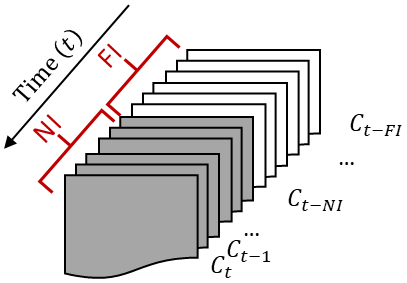
Figure 1 Illustration of the definition of near (shown in grey) and far (shown in white) daily intervals for climate variables, highlighting the far temporal interval (FI) and near temporal interval (NI) of climate data at a specific time (C_t).

2.2.2 Input climate variables

The downscaling process relies on low-resolution climate information and LR-SWE data obtained from global or regional climate models that provide the predictors for our k-NN framework. As a result, the downscaling procedure can be described by Eq. (1):

$$\begin{array}{}\text{(1)}& \begin{array}{rl}{\widehat{\mathrm{SWE}}}_{\mathrm{HR}}\left(t\right)& \approx f(T_{\min ,\mathrm{LR}}^{\mathrm{FI}},T_{\min ,\mathrm{LR}}^{\mathrm{NI}},T_{\max ,\mathrm{LR}}^{\mathrm{FI}},T_{\max ,\mathrm{LR}}^{\mathrm{NI}},\\ & P_{\mathrm{LR}}^{\mathrm{FI}},P_{\mathrm{LR}}^{\mathrm{NI}},{\mathrm{RSDS}}_{\mathrm{LR}}^{\mathrm{FI}},{\mathrm{RSDS}}_{\mathrm{LR}}^{\mathrm{NI}},{\mathrm{SWE}}_{\mathrm{LR}}\left(t\right))\end{array}\end{array}$$

Here, ${\widehat{\mathrm{SWE}}}_{\mathrm{HR}}\left(t\right)$, and SWE_LR(t) are the downscaled SWE and the LR-SWE, both at the query time (t). T_min and T_max represent the minimum and maximum temperatures, while P and RSDS denote precipitation and surface downwelling shortwave radiation. The superscript “FI” or “NI” indicates the far or near temporal intervals introduced in Fig. 1. The subscript notation (“LR”, “HR”) explicitly indicates the resolution (low resolution or high resolution). All the climate variables (T_min, T_max, P, RSDS, and SWE) are daily measurements. To ensure compatibility among datasets with varying units, all input data are rescaled to a range of 0–1 based on the absolute minimum and maximum values observed in the training dates. Hereafter, $\widehat{\mathrm{SWE}}$ refers to downscaled SWE. Details on the experiments conducted to identify the most effective climate predictors within these datasets are available in the Supplement (Table S1 and Fig. S1).

2.3 Downscaled SWE estimation

Estimating $\widehat{\mathrm{SWE}}$ for a date when HR-SWE data are not available relies on the existing HR-SWE data from the training dates. For each training date, the input variables described in Eq. (1) and their corresponding HR-SWE images are used. By utilizing a vector of inputs, we estimate $\widehat{\mathrm{SWE}}$ by selecting the k-nearest candidates in the input space.

In this study, the k-NN algorithm is applied to downscale low-resolution climate data to HR-SWE estimates by selecting training days with similar climate conditions. The flowchart (Fig. 2) illustrates the proposed downscaling method for estimating HR-SWE, and the steps are as follows:

1. Gather the input variables, including the far and near intervals of temperature, precipitation, shortwave radiation, and LR-SWE for both the target date and the training dates.

2. Calculate the distance between the input vector of the target date and the input vectors of the training dates.

3. Select the k-nearest training dates based on their proximity to the target date in the input space.

4. Retrieve the corresponding HR-SWE images associated with the selected k-nearest training dates.

5. Aggregate the retrieved HR-SWE images to estimate $\widehat{\mathrm{SWE}}$ for the target date.

The metric used to identify the nearest neighbors between a given target date (t₁) and a training date (t₂) is the multivariate Manhattan distance, described in Eq. (2):

$$\begin{array}{}\text{(2)}& d\left\{t_{\mathrm{1}},t_{\mathrm{2}}\right\}=\sum _{i=\mathrm{1}}^E{\mathit{\alpha }}_i\left|x_i\left(t_{\mathrm{2}}\right)-x_i\left(t_{\mathrm{1}}\right)\right|\end{array}$$

The weights α_i assigned to the input variables sum to 1 and are used to balance their influence in the selection of the k-nearest observations. The determination of optimal weights is further discussed in Sect. 2.4.2. Here, x_i represents each of the E estimators introduced in Eq. (1). Unlike Euclidean distance, which calculates the shortest straight-line distance, Manhattan distance computes the sum of the absolute differences between variables. This makes it more robust against outliers and better suited to handling high-dimensional datasets, such as those containing multiple climate variables. In our method, the distance is used to rank training dates according to their similarity to the target date.

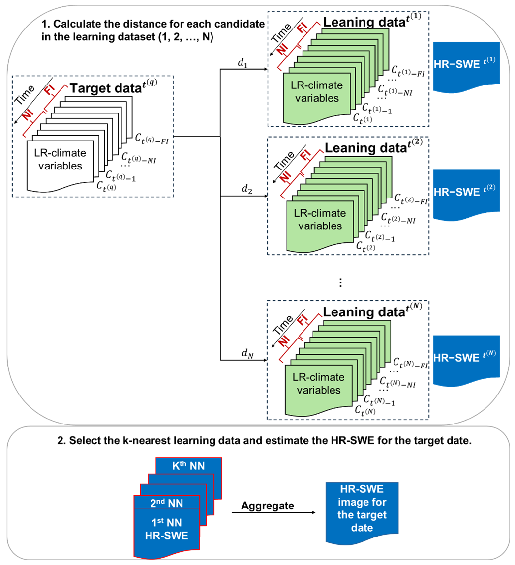
Figure 2 Flowchart depicting the proposed downscaling algorithm for estimating high-resolution snow water equivalent (HR-SWE) on a target date using low-resolution (LR) climate data: (1) gather input variables: collect the input variables, including near (NI) and far (FI) temporal intervals of climate data (e.g., temperature, precipitation) for both the target date and the training dataset. (2) Calculate distances: compute the distance (d) between the input vector of the target date and the input vectors of each candidate in the training dataset using a defined distance metric (Manhattan distance). (3) Identify k-nearest neighbors (k-NNs): rank the training data in order of increasing distances to identify the k-nearest neighbors. (4) Aggregate HR-SWE images: retrieve the HR-SWE images corresponding to the k-NNs and aggregate them to estimate the HR-SWE for the target date.

2.4 Estimating parameters and weights

To optimize parameter estimation and ensure better convergence, the parameters are estimated either using sensitivity analysis or an optimization algorithm. In this paper, the far and near intervals (FI and NI) for climate variables (Fig. 1), as well as the number of k-nearest observations, are determined using a sensitivity analysis. The weights assigned to the input features are established using an optimization algorithm.

2.4.1 Parameter sensitivity analysis

Dissimilarity, denoted as ε, is critical for determining the optimal near (NI) and far (FI) temporal intervals, as well as the optimal number of nearest observations (K), for estimating $\widehat{\mathrm{SWE}}$. This dissimilarity is quantified using the root mean squared error (RMSE), a standard measure of accuracy that reflects the average magnitude of the square of errors between the estimated and observed values. The RMSE is defined as follows:

$$\begin{array}{}\text{(3)}& \mathrm{RMSE}=\sqrt{{\displaystyle \frac{{\sum }_{i=\mathrm{1}}^N{\left({\widehat{\mathrm{SWE}}}_i-{\mathrm{SWE}}_i\right)}^{\mathrm{2}}}{N}}}\end{array}$$

where ${\widehat{\mathrm{SWE}}}_i$ is the downscaled SWE at the ith pixel, SWE_i is the reference HR-SWE at the ith pixel, and N is the total number of pixels. This formula underpins the evaluation of ε across different configurations of temporal intervals and k-nearest observation counts.

To identify the optimal temporal intervals (NI^∗ and FI^∗), we conduct a sensitivity analysis within predefined ranges, set by $\mathrm{NI}\in \left[\mathrm{1},\mathrm{7}\right]$ d and $\mathrm{FI}\in \left[\mathrm{1},\mathrm{90}\right]$ d, aiming to minimize ε. Similarly, the optimal number of nearest observations (K^∗) is determined by evaluating ε as a function of K, ranging from 1 to the maximum number of available training dates ($K\in \left[\mathrm{1},K_{\max }\right]$) to identify the configuration that yields the smallest dissimilarity between $\widehat{\mathrm{SWE}}$ and the reference HR-SWE. The maximum number of available training dates (K_max) can vary for each case study from a few days to several months.

Mathematically, the optimization processes are represented as:

$$\begin{array}{}\text{(4)}& \begin{array}{rl}& {\mathrm{NI}}^{\ast }=\underset{\mathrm{NI}}{\mathrm{argmin}}{\mathit{\epsilon }}_{\mathrm{NI}}\\ & {\mathrm{FI}}^{\ast }=\underset{\mathrm{FI}}{\mathrm{argmin}}{\mathit{\epsilon }}_{\mathrm{FI}}\\ & K^{\ast }=\underset{K}{\mathrm{argmin}}{\mathit{\epsilon }}_K\end{array}\end{array}$$

where ε_FI, ε_NI, and ε_K are the sum of RMSEs for the respective configurations, reflecting the dissimilarity between $\widehat{\mathrm{SWE}}$ (using different sizes of NI, FI, and K) and the reference HR-SWE. The only distinction between RMSE_FI, RMSE_NI, and RMSE_K is based on the varying elements (FI, NI, or K), illustrating how each influences the $\widehat{\mathrm{SWE}}$ estimate. Determining these optimal parameters enables the refinement of our SWE estimation model, enhancing its accuracy by minimizing ε.

The parameters are selected through a sensitivity analysis to minimize ε, but they do not necessarily correspond to a global optimum. This means that while they perform well in the studied regions, they may not generalize well to other locations or climatic conditions. Therefore, we recommend performing a sensitivity analysis for each region. Additionally, the sensitivity analysis assumes that the influence of these intervals is consistent across different temporal scales, which may not always be valid, particularly in regions with highly variable climate patterns. Despite these assumptions, the chosen parameters strike a balance between computational efficiency and accuracy for the downscaling task. Moreover, the subsequent weight optimization can further reduce the impact of non-global optimal parameter selection.

2.4.2 Weights optimization

The weights α_i defined in Eq. (2) are determined by minimizing the RMSE between the $\widehat{\mathrm{SWE}}$ and the reference HR-SWE using Bayesian optimization. In this model-based optimization, the global maximum or minimum of an unknown objective function is found sequentially (Shahriari et al., 2015; Snoek et al., 2012). The key aspect of this approach is the use of a probabilistic model of the response function, which is evaluated at a minimal cost through the acquisition function. The Bayesian optimization framework employs a Gaussian process prior over the objective function and iteratively refines the model through Bayesian posterior updating to determine the optimal solution.

3 Study areas, datasets, and parameters

3.1 Study areas

To evaluate the effectiveness of the proposed methodology, we selected two regions in the western United States, as indicated in Fig. 3: the California Sierra Nevada region (referred to as California) and the Upper Colorado River Basin (referred to as Colorado). These regions are heavily dependent on snowmelt as a vital source of water resources (Dawadi and Ahmad, 2012; Siirila-Woodburn et al., 2021a).

Figure 3 (a) Map of elevation (in meters) across the western United States, highlighting two regions of interest (red squares). (b) Map of the elevation and locations of in situ sites in Sierra Nevada, California. (c) Map of the elevation and locations of in situ sites in the Upper Colorado River Basin, Colorado.

In the California region, elevation ranges from a minimum of 1200 m to a maximum of 3700 m, with an average elevation of 2200 m. In the Colorado region, elevation ranges from a minimum of 1900 m to a maximum of 4300 m, with an average elevation of 3000 m. By focusing on these specific regions, we can assess the performance and applicability of the proposed methodology in other areas where snow water resources are an important component of the hydrology system.

The California Sierra Nevada snowpack plays a critical role in water resource management, contributing approximately 30 % of the state's water supply through snowmelt. However, its sensitivity to warming temperatures is evident, with the 2015 SWE on 1 April dropping to just 5 % of historical averages. This dramatic decline underscores the combined effects of reduced precipitation and higher temperatures, which exacerbate drought severity and shift the timing of water availability (Belmecheri et al., 2016).

In the Upper Colorado River Basin, snowmelt accounts for 70 %–90 % of annual streamflow, making snowpack dynamics essential to hydrological processes and water management. Heldmyer et al. (2023) identify three snow drought types, “warm”, “dry”, and “warm-and-dry”, which affect SWE and streamflow timing. Warm droughts tend to reduce SWE at lower elevations, while dry conditions cause uniform SWE reductions across elevations. These droughts advance peak streamflow timing by 7–13 d, emphasizing the region's sensitivity to climatic changes in temperature and precipitation (Heldmyer et al., 2023).

3.2 Datasets

The reference HR-SWE data, which this study aims to produce, comes from the reanalyzed SWE dataset for the western United States (Fang et al., 2022a). This dataset, captured at a 16 arcsec (∼ 500 m) resolution, covers the period from the water year (i.e., 1 October to 30 September) 1984 to 2021 and is updated daily. It combines high-resolution remotely-sensed data with a Bayesian data assimilation (Margulis et al., 2019, 2015, 2016) framework. The dataset is derived from Landsat-based fractional snow-covered area observations, is updated daily, and incorporates a land surface model to estimate SWE and snow depth. This approach enables spatially and temporally continuous SWE estimates, which are verified against in situ and lidar-derived SWE measurements for accuracy. It offers ensemble median values of SWE, calculated from a discrete probability distribution of posterior weights, thus providing an extensive and detailed view of the snow water content over the years. The dataset can be accessed at https://doi.org/10.5067/PP7T2GBI52I2 (Fang et al., 2022b). Hereafter, we refer to this dataset as the UCLA SWE. It is used as the reference dataset for training and validating our model outputs.

To obtain the necessary climatic estimators, including daily minimum and maximum air temperature, daily total precipitation, and shortwave radiation, we utilize two distinct sources: the Coupled Model Intercomparison Project (CMIP) version 6 simulations (Meehl et al., 2014; Eyring et al., 2016) and the downscaled CMIP6 over the western United States using the Weather Research and Forecasting (WRF) model (Skamarock et al., 2019) datasets (referred to as WRF-CMIP6) (Rahimi et al., 2024, 2022). The CMIP6 simulations provide daily climate data at a spatial resolution of 100 km, while the WRF-CMIP6 datasets offer high-resolution daily climate simulations at different resolutions for the western United States. In this study, we use WRF-CMIP6 dataset at a 9 km resolution. Importantly, WRF-CMIP6 and CMIP6 are used solely as sources for input climatological variables, which are used as predictors in our statistical downscaling model.

Rahimi et al. (2024) produced high-resolution regional climate projections by dynamically downscaling outputs from different CMIP6 global climate models using the WRF model. The WRF configuration was previously optimized and evaluated using ERA5 reanalysis data in Rahimi et al. (2022), which was used as a benchmark for assessing model performance under historical conditions.

While CMIP6 global models provide valuable information on large-scale climate variability and long-term trends, their coarse spatial resolution limits their ability to resolve regional weather patterns and localized climate processes. The WRF-CMIP6 dataset addresses this by dynamically downscaling CMIP6 model outputs to a 9 km grid, enhancing the simulation of regional climate variability across the western United States. This high-resolution framework offers improved regional climate projections. Utilizing both CMIP6 and WRF-CMIP6 at different resolutions enables us to investigate how using a regional configuration of a climate model that dynamically downscales CMIP6 data, and a global climate model with different spatial resolutions, affects in the accuracy of our approach.

To illustrate the effect of resolution on SWE image accuracy, Fig. 4 depicts the UCLA SWE, WRF-CMIP6, and CMIP6 images for a day in the California region.

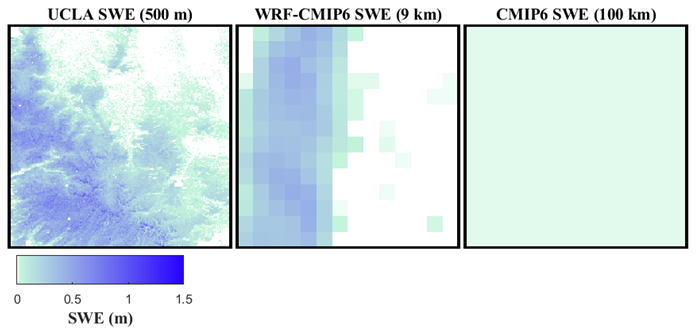
Figure 4 Comparative illustration of SWE images highlighting the effect of spatial resolution on accuracy. Displayed from left to right are the UCLA SWE, WRF-CMIP6, and CMIP6 images captured over the California region (Fig. 3b, lon: −120 to −119, lat: 38 to 39) on 8 January 1995. Distinct variations between these images underscore the influence of scaling on image accuracy.

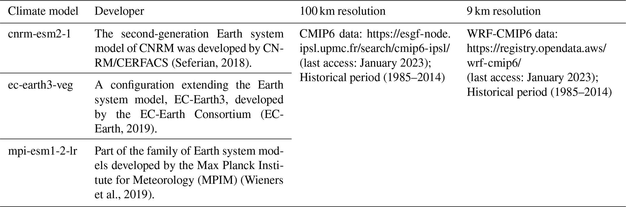
Among the available models with resolutions of both 9 and 100 km, we have selected three models for testing our methodology (Table 1). These models have been utilized in other studies (Thrasher et al., 2022; Kouki et al., 2022). Although our methodology is not limited to these models, they were selected merely as examples. Hereafter, we will refer to them as cnrm-esm2-1, ec-earth3-veg, and mpi-esm1-2.

Table 1 The climate models that are used in this study.

To ensure that the test period is not influenced by the training period, the periods 1985–2004 and 2011–2014 are designated for training dates, while the years 2005–2010 are allocated for testing. Additionally, to confirm that our testing dates are not grouped into nearly identical wet or dry categories, we employed the CONUS Drought Indices dataset (Abatzoglou, 2013). This includes drought indices derived from the 4 km daily Gridded Surface Meteorological (GRIDMET) dataset. The Standardized Precipitation Evapotranspiration Index (SPEI) is the specific drought index used in our analysis. We calculated the average aggregated SPEI for each year across each region to categorize the testing and training years in Supplement Table S2. The testing years are different in terms of the drought index.

3.3 Parameters for both case studies

Through a sensitivity analysis, we determine the NI^∗ and FI^∗ using Eq. (4). This analysis is carried out for both datasets: CMIP6 (100 km) and WRF-CMIP6 (9 km). The results of this analysis are presented in the Supplement Figs. S2 to S5, indicating that a FI^∗ of 60 d and a NI^∗ of 4 d are sufficient for accurate SWE estimation in all examined scenarios. Even though these values might not represent a global optimum, potential suboptimal effects can be considered negligible. Furthermore, these effects can also be reduced in subsequent optimization stages when determining weights.

Next, we conduct a sensitivity analysis for the parameter K^∗, the number of nearest observations, using the methodology described in Sect. 2.4.1 and Eq. (4). Figures S6 and S7 illustrate that, on average, a value of $K^{\ast }=\mathrm{130}$ is appropriate for both the California and Colorado regions. Considering the relatively small variations in accuracy, we decided not to optimize K for each dataset. Note that the value of 130 nearest observations is high. This suggests the presence of frequently repeating situations or patterns within the data. This is particularly advantageous for statistical analysis, as it provides a large number of data points, thereby improving the robustness and reliability of the results.

The optimized weights α obtained from the Bayesian optimization algorithm after 500 iterations are summarized in Table 2. Both regions exhibit similar weight patterns, with relatively high weights assigned to variables $T_{\min ,\mathrm{LR}}^{\mathrm{NI}}$, $P_{\mathrm{LR}}^{\mathrm{NI}}$, SWE_LR, and $P_{\mathrm{LR}}^{\mathrm{FI}}$.

Table 2 Weight optimization (α, in Eq. 2) results using Bayesian optimization. The numbers greater than 0.1 are highlighted in bold. This value, 0.1, is chosen because it almost represents the scenario where weights are distributed equally. “cnrm” refers to cnrm-esm2-1, “earth3” to ec-earth3-veg, and “mpi” to mpi-esm1-2.

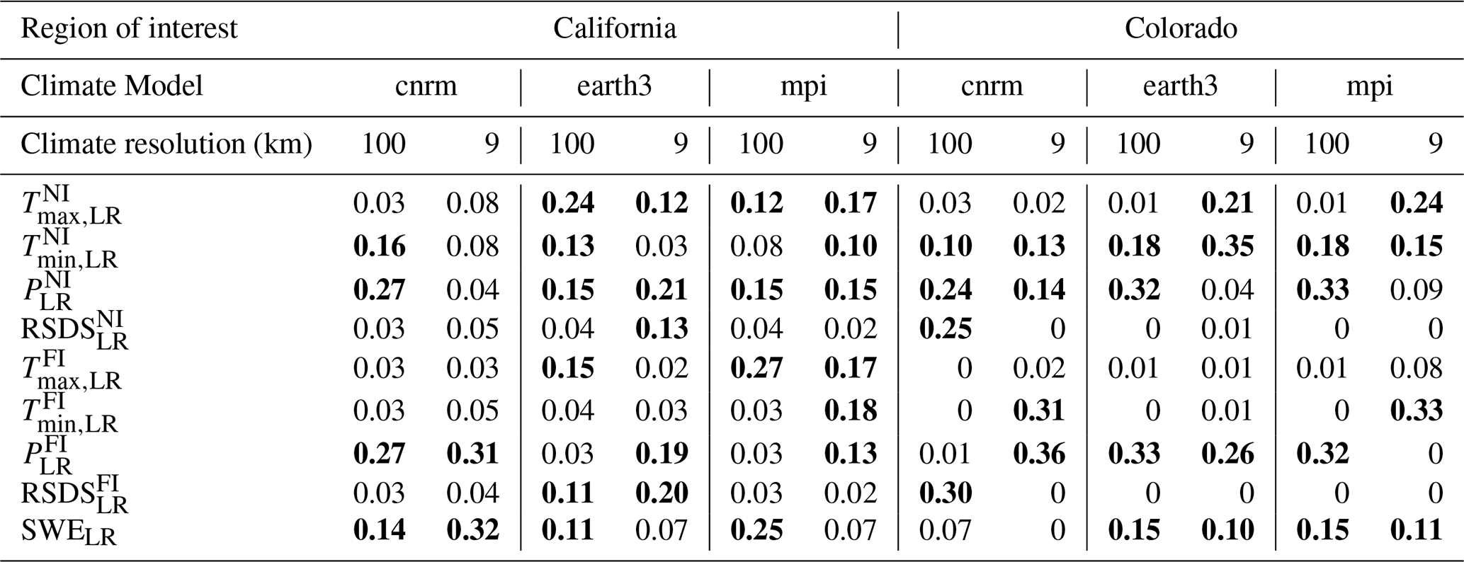
From a physical perspective, this weighting aligns with the processes governing SWE distribution and dynamics. Minimum temperature ($T_{\min ,\mathrm{LR}}^{\mathrm{NI}}$) significantly influences freezing and melting thresholds, which are critical for snowpack accumulation or reduction. Precipitation variables, both near and far intervals ($P_{\mathrm{LR}}^{\mathrm{NI}}$, $P_{\mathrm{LR}}^{\mathrm{FI}}$), directly contribute to SWE through their impact on snowfall volume. Meanwhile, the inclusion of SWE_LR as a relatively highly weighted variable can highlight its importance as an indicator.

4 Evaluation approach

Our method is evaluated through various accuracy metrics and independent datasets. First, we generate two quality metrics in conjunction with the $\widehat{\mathrm{SWE}}$ images. These metrics provide a quick assessment of the quality of the $\widehat{\mathrm{SWE}}$ products. For each target date, two quality metrics are provided: the average and the standard deviation of the similarity metric across the k best-selected SWE candidates. The lower the average and standard deviation of the similarity metric, the more accurate the $\widehat{\mathrm{SWE}}$ estimation.

4.1 Time series visualization

To further demonstrate the efficacy of our method, we showcase some SWE time series spanning 6 years at in situ locations from the Snow Telemetry (SNOTEL) network (https://www.wcc.nrcs.usda.gov/snow/, last access: January 2023). First, the pixels nearest the in situ locations are identified. Then, the SWE values at these locations in both the UCLA SWE data and other well-established SWE datasets (explained in Sect. 4.3) in the western United States are compared with the $\widehat{\mathrm{SWE}}$ values. We also present scatter plots colored by density (density scatter plots), illustrating the correlation between the reference (UCLA SWE) and $\widehat{\mathrm{SWE}}$ values at in situ locations. As in Fang et al. (2022a)'s study, SWE values below 10 mm are excluded from the comparison. This screening is done because very small SWE values (less than 10 mm) can be the result of measurement errors, minimal snow presence, or other factors that may not yield meaningful insights.

While the SNOTEL network provided the spatial locations for these comparisons, we did not use direct in situ SNOTEL SWE measurements in this analysis. The UCLA SWE dataset has been previously validated against in situ observations, including SNOTEL, and has been widely recognized as a benchmark for SWE validation in subsequent studies. For example, Ma et al. (2023) used the UCLA SWE dataset as a reference to assess the performance of machine learning approaches for estimating spatiotemporally continuous SWE. Similarly, Fang et al. (2023) used the UCLA SWE dataset as a baseline for evaluating snow water storage uncertainty. These applications highlight the dataset's reliability and its critical role in advancing snow hydrology research.

4.2 Cross-validation

We also validate our results using cross-validation. This involves removing 6 years of the UCLA SWE from the training dataset. We estimate $\widehat{\mathrm{SWE}}$ based on the remaining training data and compare the results with the reference UCLA SWE image using correlation, mean difference, and RMSE as evaluation criteria. These assessment metrics are summarized in Table S3.

In our quantitative comparison, we calculate the accuracy metrics at different elevation bands (elevation < 2000, 2000 < elevation < 3000 m, and elevation > 3000 m) and across various land cover types, including forest and non-forest areas. We utilize the MODIS Land Cover Type (MCD12Q1) Version 6.1 data for land cover information (https://lpdaac.usgs.gov, last access: January 2023, Friedl and Sulla-Menashe, 2022). This data, as of 2018, is maintained by the NASA EOSDIS Land Processes Distributed Active Archive Center (LP DAAC) at the USGS Earth Resources Observation and Science (EROS) Center in Sioux Falls, South Dakota. Elevations are derived from NASA SRTM Digital Elevation 30 m data (Farr et al., 2007).

4.3 Comparison with independent SWE datasets

To enhance the reliability of $\widehat{\mathrm{SWE}}$, additional verification is performed through comparisons with the following three independent SWE datasets. These comparisons are essential for validating the accuracy and consistency of our $\widehat{\mathrm{SWE}}$ images, using the evaluation criteria detailed in Table S3.

4.3.1 SNODAS 1 km SWE product

The first independent dataset includes the 1 km SWE data from the Snow Data Assimilation System (SNODAS), developed by the NOAA National Weather Service's National Operational Hydrologic Remote Sensing Center (NOHRSC) (Center, 2004). SNODAS is a comprehensive modeling and data assimilation system designed to provide estimates of snow cover that are crucial for hydrologic modeling and analysis. The dataset covers the period from 28 September 2003 to the present.

We first resample the $\widehat{\mathrm{SWE}}$ images by aggregating the values of all the pixels that intersect each 1 km SNODAS pixel. This ensures that both datasets have the same spatial resolution. Subsequently, we compare the SNODAS SWE products with the $\widehat{\mathrm{SWE}}$ images using the evaluation criteria introduced in Table S3. SWE pixel values less than 10 mm are not included in the comparison.

4.3.2 Daymet 1 km SWE product

The second independent dataset includes the 1 km SWE data from the Daymet V4 dataset: Daily Surface Weather and Climatological Summaries (Thornton et al., 2022). Daymet provides gridded estimates of daily weather parameters for North America, including minimum and maximum temperatures, precipitation, and SWE, with data spanning from 1 January 1980. We follow a similar procedure as in the comparison with the SNODAS SWE products.

4.3.3 University of Arizona (UA) 4 km SWE product

The third independent dataset is the 4 km SWE data provided by the University of Arizona (UA) (Broxton et al., 2019; Zeng et al., 2018). It assimilates in situ snow measurements from the SNOTEL and Cooperative Observer Network (COOP) networks (Fleming et al., 2023; National Research Council, 1998), incorporating detailed snowpack measurements. It also integrates modeled, gridded temperature and precipitation data, providing a comprehensive representation of SWE over the conterminous United States since 1981. For this comparison, we employ a similar procedure to that used in the comparisons with the previous two independent SWE products.

5 Results

5.1 Time series visualizations

To showcase the effectiveness of the proposed technique, SWE time series for a 6-year duration at the three highest-elevation in situ locations (see Table 3) in California are presented in Fig. 5 (and Supplement Fig. S8 for Colorado). These time series visually represent $\widehat{\mathrm{SWE}}$ values over time, enabling a comparison between the $\widehat{\mathrm{SWE}}$ values and the UCLA SWE, Daymet, SNODAS, and UA SWE data. The red line, representing our estimated values, generally tracks the blue line (UCLA SWE) well across the 6-year period for the three high-elevation locations. However, in some years and locations, such as at the “Leavitt Lake” and “Lobdell Lake” stations in 2005, the red line diverges slightly from the blue line, indicating variability in the accuracy of the estimates across different time periods. Nevertheless, even in 2005, our estimation is still within the range of other well-established SWE estimations. Moreover, in 2005, the other datasets do not align on the amount of SWE, indicating that this year is intrinsically challenging. This demonstrates that the proposed method can closely estimate the UCLA SWE on a point scale in most years.

Table 3 Names and locations of in situ sites.

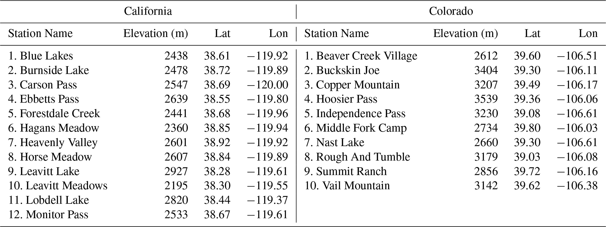
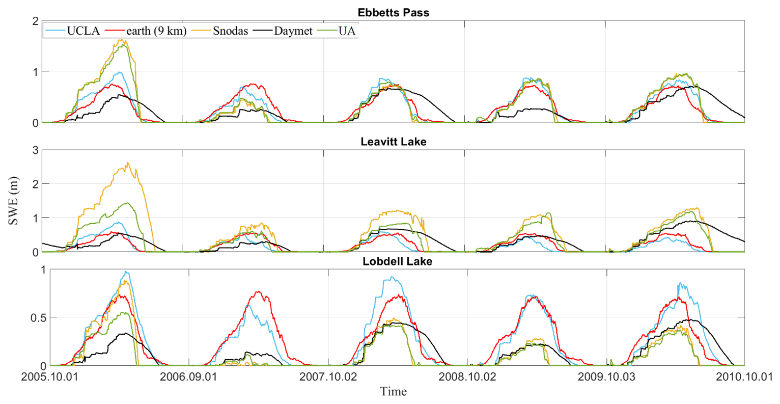
Figure 5 The SWE time series spans a 6-year period at the three highest-elevation in situ locations (Table 3) in California. “UA” represents the University of Arizona SWE datasets. The downscaled SWE ($\widehat{\mathrm{SWE}}$) results were obtained from ec-earth3-veg climate data at a 9 km resolution.

Additionally, density scatter plots are obtained using the “dscatter” function (Henson, 2024) and are illustrated in Fig. 6 for California (and Supplement Fig. S9 for Colorado), depicting the relationship between UCLA SWE and $\widehat{\mathrm{SWE}}$ values at in situ locations (see Table 3) obtained from three climate models as estimators: ec-earth3-veg, mpi-esm1-2, and cnrm-esm2-1 at both 9 and 100 km resolution.

Referencing Fig. 6, using ec-earth3-veg at a 9 km resolution as an estimator, the derived $\widehat{\mathrm{SWE}}$ in California shows a stronger correlation with the UCLA SWE at in situ locations, achieving an R value of approximately 0.87. This model also demonstrates improved accuracy, with a lower RMSE and MD (approximately 0.14 (m) for RMSE and about 0.02 (m) for MD). In contrast, as shown in Supplement Fig. S9, using cnrm-esm2-1 at a 100 km resolution as an estimator, the derived $\widehat{\mathrm{SWE}}$ in Colorado exhibits a stronger correlation with the UCLA SWE at in situ locations, marked by an R value close to 0.85, and the RMSE estimated at around 0.09 m.

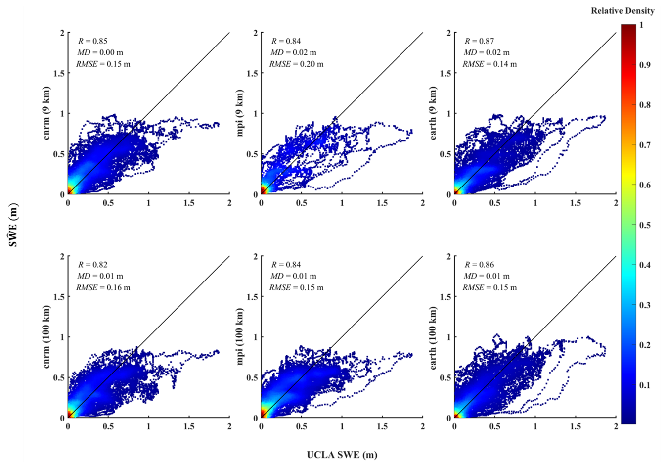
Figure 6 A density scatter plot in California from 2005 to 2010 compares in situ data locations (Table 3) from UCLA SWE images with the downscaled SWE ($\widehat{\mathrm{SWE}}$) values. The solid black line represents the 1:1 line. The displayed metrics include the correlation coefficient (R), mean difference (MD), and root mean squared error (RMSE). Only data with SWE values greater than 10 mm are included in the comparison.

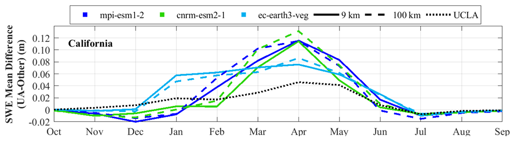
Figure 7 presents a comparison of the mean $\widehat{\mathrm{SWE}}$ and mean UCLA SWE over a 6-year period in California and Colorado. Among the models, cnrm-esm2-1 at 100 km resolution, in most months, outperforms ec-earth3-veg and mpi-esm1-2 in Colorado. In contrast, in California, ec-earth3-veg mostly exhibits superior performance at both the 9 and 100 km resolutions. However, all the models underestimate SWE in California, suggesting that testing other climate models for this region may be beneficial. Collectively, these findings emphasize the significance of selecting an appropriate model and its optimal resolution for SWE estimation.

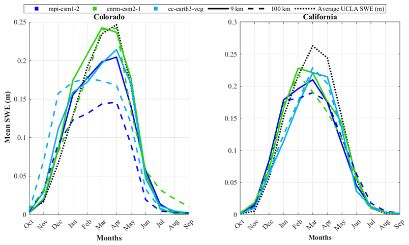
Figure 7 The average of the UCLA SWE (black dotted line, reference) and the downscaled SWEs ($\widehat{\mathrm{SWE}}$; blue and green lines) for each area over the 6-year period from 2005 to 2010 are shown. The three climate models used in the downscaling are represented by different colors: light blue for ec-earth3-veg, green for cnrm-esm2-1, and dark blue for mpi-esm1-2. Line styles indicate the spatial resolution of the climate data: solid lines correspond to results based on a 9 km resolution, and dashed lines represent results based on a 100 km resolution. The dotted black line represents the average UCLA SWE, which is the reference.

Additionally, two videos (one for each study region) have been created to showcase a side-by-side comparison of UCLA SWE and $\widehat{\mathrm{SWE}}$ images: California ($\widehat{\mathrm{SWE}}$ obtained from ec-earth3-veg at 100 km), Colorado ($\widehat{\mathrm{SWE}}$ obtained from cnrm-esm2-1 at 9 km).

Several factors explain why certain models outperform others in specific locations. While a detailed comparison of model performances across various regions is beyond the scope of this study, other studies have explored this area. For example, Kouki et al. (2022) evaluated the ability of CMIP6 models to estimate SWE across the Northern Hemisphere and found that different models perform variably in specific regions based on their ability to simulate particular climatic and geographical conditions. In terms of the contribution of temperature and precipitation to SWE biases, precipitation plays a more dominant role, especially in winter. However, temperature becomes more significant during spring, when snowmelt occurs. In regions where temperatures are closer to 0 °C, biases in temperature can substantially affect snowmelt modeling. Overall, the results underscore that precipitation is the primary driver of SWE biases in winter. However, temperature plays a crucial role during the snowmelt season in spring, particularly in regions with more temperate climates, such as the southern parts of North America and Europe.

5.2 Cross-validation

Cross-validation accuracy assessments of $\widehat{\mathrm{SWE}}$ are outlined in Supplement Tables S4 and S5. Figures 8 and 9, and Figs. S10 and S11 in the Supplement further present these assessments, considering variations in elevation and land cover for California and Colorado. Overall, for most months, using climate data with a higher resolution (9 km) as an estimator yields only slightly higher or identical accuracies compared to climate data with a lower resolution (100 km). In a broad comparison across resolutions in Colorado and California, the cnrm-esm2-1 and ec-earth3-veg models generally exhibit the best performance. Nonetheless, it is crucial to recognize variability in model performance across different regions. For instance, in both California and Colorado, all models generally perform better or comparably at higher elevations (elevation > 3000 m) compared to medium elevations (2000 m < elevation < 3000 m). While RMSE values tend to be smaller at lower elevations due to lower SWE magnitudes, accuracy at higher elevations is more hydrologically significant, as these zones contribute the majority of seasonal snowmelt runoff.

In Colorado, all models exhibit comparable performance in both forested and non-forested areas. In contrast, in California, models tend to perform slightly better in non-forested areas. Moreover, Figs. 9 and S11 illustrate the average spatial error in March and May, respectively, for California and Colorado. In California, $\widehat{\mathrm{SWE}}$ underestimates reference SWE, with the extent of underestimation varying across different climate models. For instance, in California, cnrm-esm2-1 at 9 km achieves the lowest underestimation. In general, the cnrm-esm2-1 model at 9 km performs better as an estimator for Colorado, with a mean RMSE of 0.07 m and a standard deviation of 0.05 m. Conversely, for California, the ec-earth3-veg model at 9 km provides the highest accuracy, yielding a mean RMSE of 0.13 m and a standard deviation of 0.1 m.

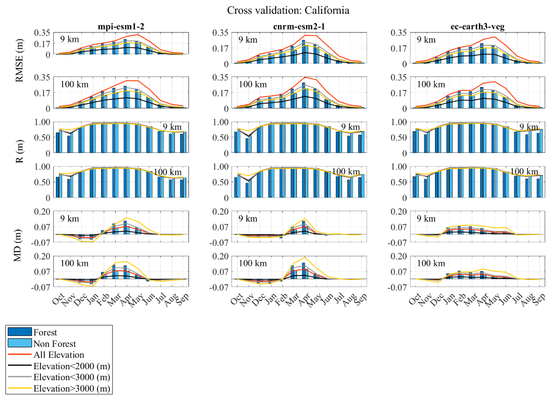
Figure 8 Accuracy assessment of downscaling cross-validation over the 6-year period from 2005 to 2010, conducted in California. Column titles indicate the results for the downscaled SWE ($\widehat{\mathrm{SWE}}$) using the respective climate models as estimators. “9 km” and “100 km” refer to the resolutions of the climate data. The evaluation metrics include the correlation coefficient (R), mean difference (MD), and root mean squared error (RMSE). These metrics are considered in different elevation values and different land covers. In the legend, 2000 m < elevation < 3000 m is shown as elevation < 3000 m.

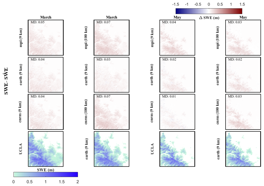
Figure 9 Spatial assessment of the downscaling. The first three rows represent the mean difference between the UCLA SWE and downscaled SWE (SWE − $\widehat{\mathrm{SWE}}$) over California throughout the 6-year testing period (2005–2010) for two months (March and May). The last row represents the averaged reference SWE (UCLA SWE) or averaged downscaled SWE ($\widehat{\mathrm{SWE}}$) throughout the 6-year testing period (2005–2010) for two different months (March and May). The evaluation metric includes mean difference (MD).

5.3 Comparison with 1 km SWE SNODAS dataset

The comparison of the UCLA SWE and $\widehat{\mathrm{SWE}}$ with the 1 km resolution SNODAS dataset is presented in Supplement Table S6, Figs. 10 and 11, and Figs. S12 and S13.

In California, during the snowiest months, the ec-earth3-veg estimator excels in terms of RMSE, correlation, and mean difference at both resolutions. In Colorado, the mpi-esm1-2 estimator mostly demonstrates superior performance. Interestingly, in Colorado, the 100 km resolution slightly outperforms the 9 km resolution across some models, but in others, the 9 km resolution marginally surpasses the 100 km resolution. In other words, in our experiments, SWE downscaling performance using 100 km CMIP6 inputs was in some cases comparable to using 9 km WRF-CMIP6 climate predictors, though higher resolution inputs typically offered modest improvements. According to Figs. 11 and S12, generally, in California, the ec-earth3-veg model outperforms others at both 9 and 100 km resolutions in both March and May, although it tends to underestimate SWE. In contrast, in Colorado, the mpi-esm1-2 model at 9 km performs better in March and May, and it mostly overestimates SWE. In general, in Colorado, the mpi-esm1-2 model at 100 km showed the most favorable results, with a mean RMSE of 0.08 m and a standard deviation of 0.07 m. In California, the ec-earth3-veg model at 9 km achieved the best performance, with a mean RMSE of 0.23 m and a standard deviation of 0.20 m.

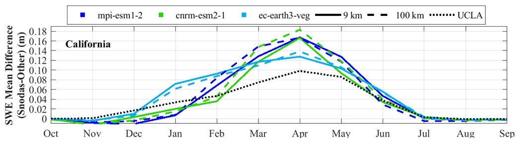
Figure 10 The average mean difference of SWE over California for the 6-year testing period (2005–2010) compares UCLA SWE (black dotted line) and downscaled SWE ($\widehat{\mathrm{SWE}}$) data (blue and green lines) against SNODAS. The $\widehat{\mathrm{SWE}}$ data, derived from different climate models, are represented by distinct colors: light blue for ec-earth3-veg, green for cnrm-esm2-1, and dark blue for mpi-esm1-2. Solid lines indicate estimates at a 9 km resolution, while dashed lines correspond to a 100 km resolution, distinguishing the spatial resolutions of the climate data.

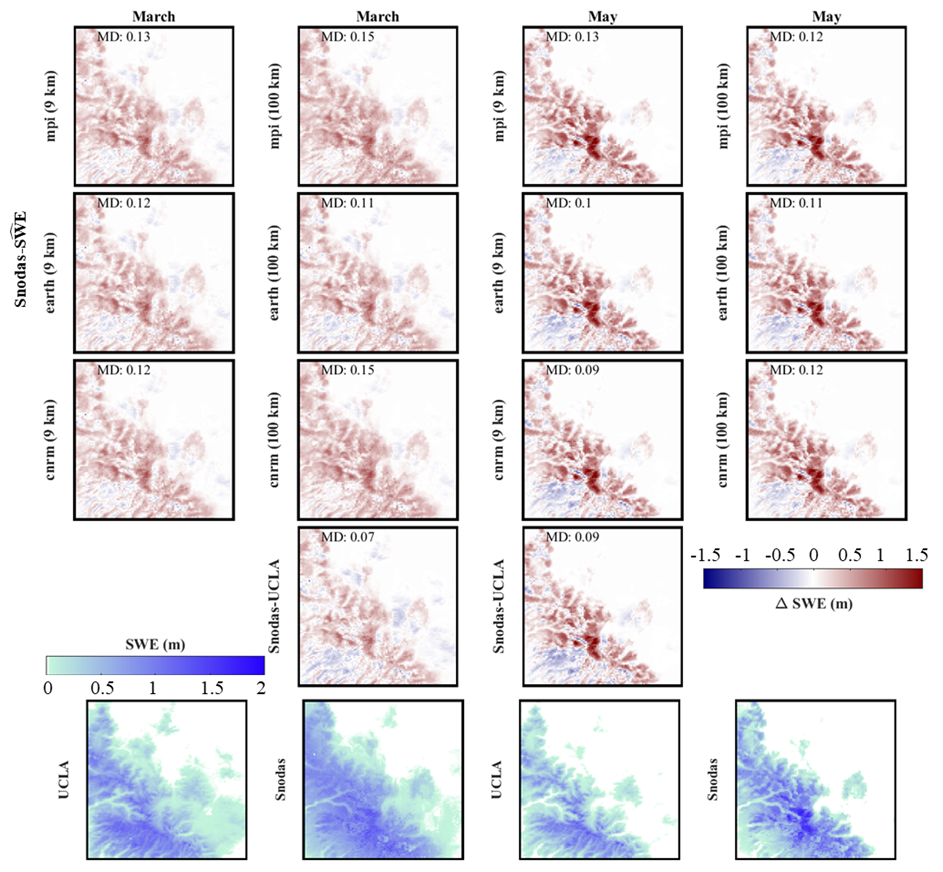
Figure 11 Comparison with SNODAS data. The first four rows present the average difference between SNODAS and downscaled SWE ($\widehat{\mathrm{SWE}}$) or UCLA SWE (SNODAS-$\widehat{\mathrm{SWE}}$ or SNODAS-UCLA) over California for March and May during the 6-year testing period (2005–2010). The last row compares the average UCLA SWE or SNODAS SWE over California for March and May during the same 6-year testing period (2005–2010). The evaluation metric includes mean difference (MD).

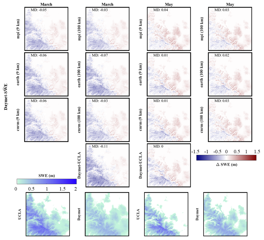
5.4 Comparison with 1 km SWE Daymet dataset

This section presents a comparison of $\widehat{\mathrm{SWE}}$ from the three climate models with the 1 km SWE data from the Daymet dataset. Supplement Table S7, along with Figs. 12 and 13,and Figs. S14 and S15 present the comparison of UCLA SWE and $\widehat{\mathrm{SWE}}$ against the 1 km SWE Daymet dataset.

In California, the ec-earth3-veg model leads in performance at both the 9 and 100 km resolutions, boasting the lowest RMSE and highest correlation. For Colorado, the cnrm-esm2-1 estimator predominantly demonstrates superior performance. When comparing both the UCLA SWE and $\widehat{\mathrm{SWE}}$ to the 1 km SWE Daymet dataset, the results indicate a close alignment between the two datasets . Figures 13 and S13 demonstrate that in California and Colorado, during the months of March and May, the cnrm-esm2-1 estimator yields the best results. In both regions, this model tends to overestimate SWE in March and underestimate it in May. In general, the cnrm-esm2-1 estimator at 100 km is the most accurate for Colorado, presenting a mean RMSE of 0.11 m and a standard deviation of 0.04 m. For California, the mpi-esm1-2 model at 100 km performs best, with a mean RMSE of 0.19 m and a standard deviation of 0.06 m. However, ec-earth3-veg achieves the same mean RMSE, with a standard deviation of 0.07 m.

Figure 12 Same as Fig. 10, but for comparison against the Daymet data.

Figure 13 Same as Fig. 11, but for comparison against the Daymet data.

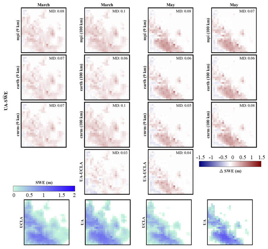
5.5 Comparison with 4 km SWE from the University of Arizona dataset

This section compares the $\widehat{\mathrm{SWE}}$ from three models against the 4 km SWE data from the University of Arizona (UA). Supplement Table S8, Figs. 14 and 15, and Figs. S16 and S17 present the comparison of UCLA SWE and $\widehat{\mathrm{SWE}}$ with the 4 km SWE data from the UA dataset.

A deeper analysis of model performance highlights differences. In Colorado, the cnrm-esm2-1 estimator stands out at both 9 and 100 km resolutions. Meanwhile, in California, the ec-earth3-veg model mostly surpasses other models, achieving the lowest mean RMSE at both resolutions.

Overall, the 9 km resolution slightly outperforms the 100 km resolution in both states. This suggests that a finer resolution might yield slightly more precise $\widehat{\mathrm{SWE}}$ estimates. Additionally, when comparing UCLA SWE and $\widehat{\mathrm{SWE}}$ to the 4 km UA SWE, the results demonstrate a tight congruence between the two datasets. Furthermore, Figs. 15 and S15 show that in California, for March and May, the ec-earth3-veg model at a 100 km resolution performs better. Meanwhile, in Colorado, the cnrm-esm2-1 estimator performs best in these two months. The ec-earth3-veg model tends to underestimate SWE in California, while in Colorado, cnrm-esm2-1 generally overestimates SWE in May. In general, the cnrm-esm2-1 estimator at the 9 km scale provides the best results for Colorado, having a mean RMSE of 0.07 m and a standard deviation of 0.05 m. In California, the ec-earth3-veg estimator at the 9 km scale is the most precise, with a mean RMSE of 0.14 m and a standard deviation of 0.13 m.

Figure 14 Same as Fig. 10, but for comparison against University of Arizona (UA) data.

Figure 15 Same as Fig. 11, but for comparison against University of Arizona (UA) data.

6 Discussion

In general, using the cnrm-esm2-1 model as an estimator results in better accuracy in Colorado at both the 100 and 9 km resolutions compared to other models. For instance, in Colorado, the use of the cnrm-esm2-1 model at a 9 km resolution demonstrated close agreement with the observed SWE, with an average RMSE of 0.07 m. This performance highlights the model's strong compatibility with the climatic and geographical complexities of Colorado. Conversely, in California, the ec-earth3-veg model excels at a 9 km resolution, providing the most accurate results with an average RMSE of 0.13 m compared to the reference datasets. This suggests that its higher resolution better captures the region's complex environmental and topographical variations.

It also appears that the finer resolution of 9 km provides slightly better accuracy than the 100 km resolution across all models, although the difference is not substantial. However, the difference between 9 and 100 km inputs can vary by region and model.

This underscores the importance of selecting an appropriate climate model for SWE estimation, beyond merely choosing a higher-resolution model. Moreover, CMIP6 models are designed for long-term climate projections and capture broad climate trends rather than predicting specific weather events. Despite this, the downscaled SWE using the proposed approach based on CMIP6 inputs, in some cases, can be comparable to those using WRF-CMIP6 climate predictors, which dynamically downscale CMIP6. This can be largely because the proposed methodology relies on long-term climate data through the use of far and near temporal intervals, and CMIP6 effectively captures broad climatic trends and seasonality, including changes in temperature and precipitation patterns. This comparison emphasizes that model selection and input quality are key drivers for SWE estimation performance, sometimes more than input resolution alone. Accordingly, achieving an accurate HR-SWE estimation relies significantly on the choice and accuracy of the climate model inputs, such as precipitation and temperature data. As a result, the accuracy of the downscaled SWE remains highly sensitive to biases in these input variables. For example, precipitation biases can be a dominant factor influencing SWE estimation errors, and temperature biases can become more significant during transitional periods, such as the spring melt season. While we test both CMIP6 and WRF-CMIP6 climate variables as inputs, a full comparison to downscale SWE is beyond the scope of this study.

The following comparison provides a broader perspective on how our proposed method compares with other statistical downscaling techniques. BCSD methods are effective in reducing uncertainties in climate model outputs by adjusting model biases using high-resolution observations. These methods are particularly valuable for ensuring that model outputs align with observed climatology and capture local variability. However, they depend heavily on the availability of high-quality in situ data, which limits their application in remote or data-sparse regions. In contrast, our method excels in areas with sparse data, as it uses low-resolution climate data without requiring ground observations, making it adaptable to a broader range of conditions.

Analog-type statistical downscaling approaches offer a simple, computationally efficient way to project high-resolution data based on historical relationships between large-scale climate patterns and local climate variables. These methods are useful in regions where historical climate patterns are stable and well-documented. On the other hand, our method introduces several key improvements over traditional k-NN downscaling techniques. First, the adaptation of the k-NN approach through the incorporation of far and near temporal intervals of climate data enhances its ability to handle dynamic variables such as snow, which are subject to significant changes due to climate variability. Unlike conventional analog methods, which constrain analog candidates to a specific temporal window near the query date, this method eliminates such restrictions.

This flexibility is crucial for three reasons: (1) the inclusion of far and near temporal intervals allows the selection of the most suitable candidates across a broader temporal range, eliminating the need for narrow constraints; (2) this flexibility may help preserve rare but important extreme events in the downscaled data, since restricting candidates to a narrow temporal window increases the risk of excluding suitable analogs.; and (3) it facilitates downscaling for the periods where no exact analogs exist in the historical record within a specific date range. Instead, suitable analogs may still be found in the historical data, but during different periods. For instance, as climate change progresses, a day in winter may no longer have a match on the same calendar day in the past. Instead, an analog might be found on another calendar day, such as in a warmer season like fall or spring.

Using very low-resolution climate data as input reduces both memory requirements and computation time compared to physical snow models, which also require high-resolution climate data as input to estimate HR-SWE. This efficiency enables the generation of HR-SWE estimates over large spatial domains with reduced computational overhead. This is particularly beneficial when applying the method to large areas, long temporal scales, or ensembles of climate data.

7 Conclusion

This research proposes a methodology to downscale low-resolution daily snow water equivalent (LR-SWE) by utilizing low-resolution daily climate data to produce daily, high-resolution SWE (HR-SWE) data, covering the period from 1950 to the present. We test our approach in two distinct areas (California and Colorado) in the western United States. Utilizing existing low-resolution climate factors obtained from global CMIP6 climate data (100 km), downscaled CMIP6 for the western United States (WRF-CMIP6, 9 km), and available 500-meter HR-SWE images from 1984 to 2021 (UCLA SWE dataset) for the western United States, we implement a downscaling algorithm to estimate HR-SWE images. WRF-CMIP6 is a regional configuration of a climate model that dynamically downscales CMIP6 data to enhance spatial resolution. Utilizing both CMIP6 and WRF-CMIP6 at different resolutions as input estimators for our k-NN statistical downscaling framework enables us to assess the impact of using a regional climate model that dynamically downscales CMIP6 data, alongside a global climate model with different spatial resolutions, on the accuracy of our approach. We also select three climate models (ec-earth3-veg, mpi-esm1-2, and cnrm-esm2-1) for testing the proposed method using different models.

To perform a comprehensive accuracy assessment, we compared the downscaled SWE ($\widehat{\mathrm{SWE}}$) with established datasets like the 1 km SWE Daymet, 1 km SWE SNODAS, and the 4 km SWE from the University of Arizona. Moreover, we performed cross-validation accuracy assessments. Our $\widehat{\mathrm{SWE}}$ data closely mirrored reference HR-SWE conditions. Even when using lower-resolution climate datasets like CMIP6 (100 km), the method in some cases remained robust, leveraging recurring SWE patterns and climate data to generate more detailed SWE images.

A comprehensive analysis over all months reveals notable patterns in the performance of various climate models at different resolutions in California and Colorado. Overall, the cnrm-esm2-1 model tends to provide higher accuracy in Colorado when used as an estimator, outperforming other models at both the 100 and 9 km resolutions. In contrast, the ec-earth3-veg model performs best in California at a 9 km resolution. A finer resolution (9 km) generally offers slightly better accuracy than a 100 km resolution across models, though the difference is modest, emphasizing the importance of model selection over merely increasing resolution. However, the difference between the 9 and 100 km climate inputs can vary by region and model.

Ongoing research will focus on applying our downscaling framework to predict HR-SWE based on future climate predictions. The data generated could be invaluable not only in climate change studies but also for water resources management. This underscores the need for precise model selection and the potential for applying our findings to future climate scenarios, improving water resource management amid climate change. Moreover, our approach may be applicable in regions where high-resolution SWE data are available for certain years, but high-resolution meteorological data are limited or unavailable. However, it would require region-specific sensitivity analysis and weight optimization.