Enhancing physically based and distributed hydrological model calibration through internal state variable constraints

Accurately representing hydrological processes remains a major challenge in hydrological modeling. Recent studies have demonstrated the benefits of multi-variable calibration, which integrates additional hydrological variables such as evapotranspiration and soil moisture alongside streamflow to improve model realism. However, groundwater recharge as a calibration variable remains relatively underexplored.

This study evaluates how incorporating groundwater recharge into the calibration of the Water Balance Simulation Model (WaSiM) affects hydrological variables representation. Three configurations were tested: Baseline (BL) with streamflow-only calibration, Physical Groundwater Model (GW) with physically-based groundwater flow, and Physical Groundwater with Recharge Calibration (GW-RC), which further constrains groundwater recharge during calibration. The models were calibrated and applied to 34 catchments in Southern Québec. Their performance was evaluated using the Kling-Gupta Efficiency (KGE) for streamflow and spatial estimates of groundwater recharge derived from a previous research project conducted in the same region.

Results indicate that while calibrating on streamflow alone produces high KGE values (median KGE = 0.83 for GW and 0.82 for BL), but it comes at the cost of misrepresenting subsurface hydrological processes. Adding groundwater recharge constraints (GW-RC) reduce streamflow performance, with a median KGE of 0.77 for GW-RC, but improves hydrological variable representation, especially in seasonal runoff patterns, where it better captures the balance between surface runoff and interflow during snowmelt. Additionally, GW-RC showed the smallest differences with the groundwater recharge estimates.

These findings illustrate the consequence of equifinality in streamflow-based calibration, where multiple parameter sets can yield similar streamflow outputs while misrepresenting internal hydrological processes. Incorporating groundwater recharge constraints improves the representation of internal hydrological processes while maintaining strong streamflow simulation performance, which could ultimately enhance reliability of climate change adaptation and water resource management strategies.

1 Introduction

Accurately representing watershed processes under climate change remains a central challenge in the evolving field of hydrology (Persaud et al., 2020). Recent advances in hydrological modeling have offered valuable insights into water resource management and climate adaptation strategies (Xu et al., 2005; Chen et al., 2011; Wang et al., 2023). However, the complexity of watershed dynamics, especially in snow dominated catchments, necessitates models that can accurately simulate both surface and subsurface hydrological processes (Chu and Shirmohammadi, 2004; Farjad et al., 2016).

The need for detailed, physically based hydrological modeling goes beyond immediate concerns of water management and climate impact assessments. Groundwater dynamics are crucial for forest health (Le Maitre et al., 1999; Jacobs, 2003), as stable water availability supports ecosystem resilience (Cunningham et al., 2011; Orellana et al., 2012). By enhancing the accuracy of groundwater simulation and recharge calibration, we can improve our ability to forecast forest growth and resilience under changing climatic conditions (Ford et al., 2011; Grant et al., 2013). This linkage underscores the importance of detailed hydrological modeling and aligns with broader environmental, economic, and ecological management goals aimed at sustaining forest productivity in the face of environmental change. This approach helps forest managers make informed decisions, supporting the long-term health and sustainability of forest ecosystems (Vose et al., 2011; Sun et al., 2023).

The Water balance Simulation Model (WaSiM) (Schulla, 2021) is a distributed and physically based hydrological model. It stands out for its complexity, fine spatial resolution and comprehensive approach to modeling hydrological processes. This makes the model especially useful for analyzing intermediate hydrological variables with greater reliability. Several studies exemplify the application of WaSiM for examining internal hydrological variables across diverse geographic settings and scenarios. For example, Jasper et al. (2006) analyzed summer soil water pattern shifts due to climatic changes, demonstrating that WaSiM could effectively model the substantial alterations in hydrological responses to varying climate scenarios. Natkhin et al. (2012) used WaSiM to differentiate the impacts of climate change and forest growth dynamics on groundwater recharge in Northeast Germany. Similarly, two separate studies (Rößler and Löffler, 2010; Rössler et al., 2012) analyzed soil moisture dynamics using WaSiM, discussing the modeling potentials and limitations in high mountain catchments and the broader impact of climate on soil moisture. Bormann and Elfert (2010) investigated how land use changes influence various runoff generation processes such as surface runoff, interflow, and baseflow. Furthermore, Förster et al. (2017, 2018) conducted detailed comparisons of internal state variables with actual forest measurements, including meteorological variables and snow cover dynamics, highlighting the refined capabilities of WaSiM to model complex interactions like snow cover and canopy interception. These studies collectively demonstrate the model's utility in capturing a wide range of hydrological variables.

Despite recent advances, hydrological modeling still faces challenges in representing watershed dynamics. These challenges are especially evident when calibration relies only on streamflow data (Mei et al., 2023; Schäfer et al., 2023; De Lima Ferreira and da Paz, 2024; Pool et al., 2024). While streamflow is a key indicator for capturing temporal fluctuations in water systems, it offers limited insights into the internal hydrological processes (Rajib et al., 2018). This reliance on streamflow can result in models that perform well in reproducing observed flows but misrepresent underlying processes. This phenomenon, known as equifinality, occurs when different parameter sets produce the same outputs but for the wrong reasons (Kirchner, 2006; Yassin et al., 2017; Acero Triana et al., 2019; Mei et al., 2023). Therefore, focusing only on streamflow in model calibration can hide important differences in how hydrological processes are represented.

In pursuit of better representing hydrological processes at the catchment scale, several studies have explored hydrologic scaling and parameter transferability (Samaniego et al., 2010, 2017; Mizukami et al., 2017; Imhoff et al., 2020). Notably, Samaniego et al. (2010) introduced the multiscale parameter regionalization to tackle overparameterization and the non-transferability of parameters across different scales. Ficchì et al. (2019) also proposed a model structure that considers flow accuracy and fluxes match on different modelling timesteps, adjusting the structure and parameters to ensure robust simulation across various time scales. Additionally, Peters-Lidard et al. (2017) advocated for adopting the fourth paradigm of data-intensive science in hydrology, which leverages emerging datasets to refine our understanding of hydrological models and processes. This paradigm suggests that advancements in computational science represent a new methodological branch alongside empiricism, theory, and computational simulation. By enabling the intensive use of data, these advancements can revolutionize science by facilitating the discovery and testing of theories and models. This approach emphasizes the integration of comprehensive datasets and computational tools into conventional scientific workflows, thereby enhancing the capacity for scientific innovation and synthesis in hydrology.

Recent studies have advocated for a shift towards integrating additional hydrological variables and data sources, such as remote sensing products and in-situ measurements, into the calibration process (Dembélé et al., 2020; Meyer Oliveira et al., 2021; Liu et al., 2022; Mei et al., 2023; Schäfer et al., 2023; De Lima Ferreira and da Paz, 2024; Pool et al., 2024). Mei et al. (2023) found that including gridded soil moisture alongside gauged streamflow improved evapotranspiration simulations across 20 catchments in the Lake Michigan watershed. Schäfer et al. (2023) used WaSiM to simulate the water balance of a forested catchment in Germany, showing that including plant-available water and evapotranspiration data significantly enhanced model accuracy. De Lima Ferreira and da Paz (2024) similarly improved model performance by incorporating actual evapotranspiration estimates into a hydrological model of a Brazilian semi-arid basin, highlighting the benefits of multi-variable calibration and the need to test distinct data sources.

Although many studies have successfully used variables such as soil moisture, evapotranspiration, and groundwater head in model calibration, there remains a gap in understanding how other variables, like groundwater recharge, can improve the representation of hydrological processes. Addressing this gap is important for both the theoretical advancement of hydrological sciences and the practical applications of water resource management, flood risk assessment, and climate change mitigation (Pradhan and Indu, 2019). By adopting a calibration approach that integrates a more holistic view of watershed processes, models become more reflective of complex hydrological interactions and gain robustness in the face of non-stationary climate conditions (Wang et al., 2023). This enhanced process representation and strengthens confidence in model projections, making them more reliable for future applications.

In this study, we implement three distinct model configurations of the WaSiM hydrological model: Baseline (BL), which follows a traditional streamflow-based calibration; Physical Groundwater Model (GW), which introduces physically based groundwater flow processes; and Physical Groundwater with Recharge Calibration (GW-RC), which further constrains groundwater recharge during calibration. The objective is to investigate how different calibration strategies and levels of model complexity influence the representation of hydrological processes over a set of 34 catchments in snowy catchment conditions. Through comparative analysis of these configurations, we aim to expose the nuances in model performance and hydrological variable representation, contributing to the ongoing debate on the best practices for hydrological model calibration.

2 Methods

2.1 Study area

This study examines 34 catchments in Southern Quebec, Canada, each with distinct physiographic and hydrometeorological features. The catchments range in size from 525 to 6840 km² (see Fig. 1). These catchments were selected based on several key criteria to ensure robust model calibration and validation. Specifically, they were selected based on the availability of comprehensive streamflow data from 1981 to 2010. Additionally, catchments were selected to represent the region's geographical and hydrological diversity to capture a range of climatic conditions across the study area. Where possible, catchments covered by the PACES project (see detail in Sect. 2.2.5) were prioritized to ensure data consistency and facilitate comparisons of groundwater recharge estimates. To preserve the natural integrity of hydrological processes under study, selected catchments needed to be free from dams and reservoirs and located away from major urban areas to minimize anthropogenic influences.

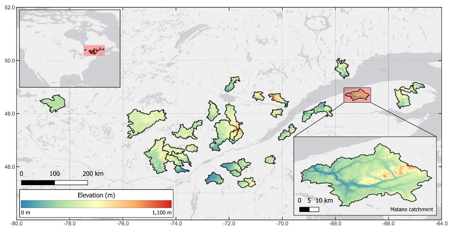
Figure 1 Elevation map of study catchments in southern Quebec. Base map created using ArcGIS^® software by Esri (©Esri, all rights reserved).

The Köppen-Geiger Climate Classification designates most of the study area (28 catchments) as belonging to class Dfb (humid continental mild summer, wet all year), except a small part (six catchments) located in the northern portion that belongs to class Dfc (subarctic with cool summers and year-round precipitation) (Beck et al., 2018). The region experiences four distinct seasons. Winters are characterized by frequent sub-freezing temperature and significant snowfall. As spring arrives, temperatures gradually rise, leading to significant snowmelt which, along with increasing rainfall, influences streamflow and water availability. Summer brings warmer temperatures, peaking in July, with rainfall remaining relatively high. Fall sees a gradual cooling and a transition from rain to increasing snowfall, setting the stage for another winter cycle. This climatic diversity induces complex hydrological processes at catchment scale, as the interplay between snowmelt and precipitation patterns has a significant influence on streamflow and water availability. These patterns are not unique to Québec but are indicative of broader hydrological changes occurring across boreal regions globally under climate change.

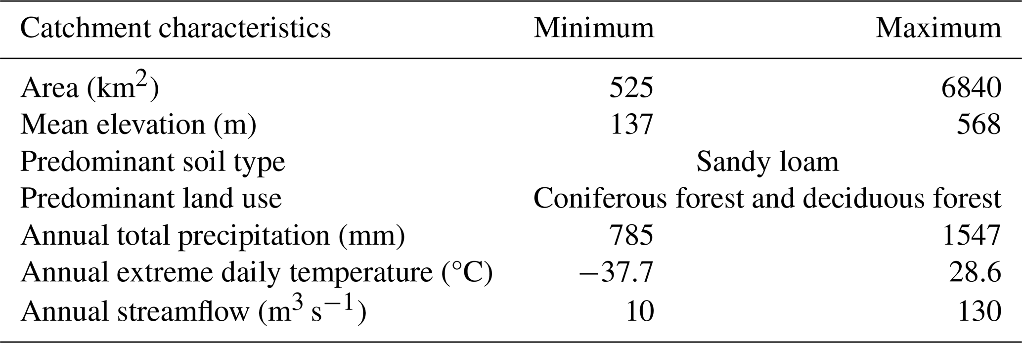
To contextualize the environmental and hydrological setting of the selected catchments, Table 1 presents a synthesis of key descriptors. The table shows the minimum and maximum values for a set of hydrological and geophysical characteristics for each catchment, providing an at-a-glance perspective of the environmental variation within the study area.

Table 1 Hydrological and geophysical characteristics of the study catchments.

2.2 Data

2.2.1 Hydrometeorological data

This study utilizes meteorological data, specifically total precipitation and mean temperature on a daily time step, sourced from ECMWF's Reanalysis v5 (ERA5) (Hersbach et al., 2020). While ERA5 is known to underestimate winter precipitation and exhibit biases in convective precipitation, studies such as Tarek et al. (2020) have demonstrated that ERA5-driven hydrological simulations perform comparably to those using ground-based observational data across Eastern Canada. Their evaluation of 3138 North American catchments found that ERA5-based simulations achieved similar accuracy levels to traditional meteorological observations in hydrological modeling, particularly in Eastern Canada. While observational data can offer higher local accuracy, it also comes with gaps and inconsistencies due to station distribution and measurement errors. ERA5 provided gridded and consistent meteorological inputs across all study catchments, reducing potential biases from heterogeneous station networks. The collected meteorological data spans the period from 1981 to 2020.

Observed streamflow data from 1981 to 2010 was used, recorded at a daily resolution. This data was obtained from the Hydroclimatic Atlas of Southern Québec (MDDELCC, 2022). The dataset contains occasional gaps, primarily during winter months when ice cover and ice jams can significantly distort river flow measurements. To ensure the accuracy of the study, these periods were excluded from the dataset.

2.2.2 Elevation data

A hydrologically conditioned digital surface model was derived from the NASA Shuttle Radar Topography Mission version 3.0 Global 1 (SRTM-DSM) to account for terrain elevation. The SRTM-DSM, originally having a spatial resolution of 30 m at the equator, underwent resampling to 50 m resolution and filtering using multiple moving average windows to mitigate the impact of local noise, which could lead to erroneous hydrological behaviours (MacMillan et al., 2000). To ensure hydrological consistency, we applied hydrological corrections based on data from provincial agencies (Géobase du réseau hydrographique du Québec (GRHQ) – Données Québec, 2016). To maintain hydrological consistency, we adjusted elevation values along streams by lowering them by 5 m using the SAGA GIS software (Conrad et al., 2015). The resulting DSM accurately captures the hydrological characteristics of the study area and is used for catchment delineation. Additionally, the DSM was resampled to spatial resolutions of 250 and 1000 m. This resampling process was conducted to optimize computational efficiency while preserving the essential characteristics of the catchments. The minimum value resampling method was used to preserve hydrological connectivity within the study area.

Following this, the Tanalys software (Schulla, 2021) was used to generate key topographic layers, including slope, aspect, and river depth, all formatted for hydrological modeling within WaSiM.

2.2.3 Soil type data

To capture the spatial variability of soil hydraulic properties, we utilized the SIIGSOL 100 m database (Sylvain et al., 2021), which provides information on soil composition. The SIIGSOL database provides detailed descriptions of the proportions of sand, clay, and silt within the soil profile (MRNF, 2020). In this study, we converted the reported proportions of sand, silt, and clay layers into soil texture classes based on the classification system of the United States Department of Agriculture (USDA). The USDA soil classification system categorizes soils into various texture classes such as loam, clay, sand, silt, and combinations thereof, which are determined based on the percentage composition of each type. This classification aids in understanding the soil's physical characteristics which are crucial factors in hydrological modeling and in predicting soil-water interactions in the studied catchments (Weil and Brady, 2008).

We derived soil hydraulic properties from generated soil type maps, using established relationships between soil texture classes and hydraulic parameters. For the soil type maps, WaSiM generates soil layers of specified thickness based on the control file settings. By default, if there is only one soil type present in the catchment, the soil depth is uniformly distributed throughout the entire area. To account for soil depth variability, we divided soil types into three distinct sections based on their relative elevation within catchment: narrow, normal, and deep. Pixels with elevations below the 33rd percentile were classified as deep, while those with elevations above the 66th percentile were classified as shallow. The remaining soil type rasters fell into the normal category. This classification was based on the imperfect but useful hypothesis that higher elevations correspond to a closer proximity of bedrock to the surface, while lower elevations indicate a greater depth of soil cover in a post-glacial landscape (Akumu et al., 2016; Jeong et al., 2022).

2.2.4 Land use data

For land use attribution, we used the 2015 North American Land Change Monitoring System (NALCMS) 30 m land cover dataset (Latifovic et al., 2012; Commission for Environmental Cooperation, 2015). The classification scheme used in this map adheres to the widely recognized Land Cover Classification System (LCCS) standard established by the Food and Agriculture Organization (FAO) of the United Nations. This standardized approach ensures the consistency and comparability of land cover information, enabling meaningful regional scale assessments and studies. The nearest neighbor resampling method was employed to align land use maps with the other raster maps used in WaSiM. Land use exerts a substantial influence on various hydrological parameters, and more specifically for the context of this study, it significantly affects parameters such as root distribution, vegetation cover fraction (VCF), roughness length (Z0), and albedo within the hydrological model. The distribution and characteristics of land cover types, ranging from forests to urban areas, directly impact these parameters, thereby influencing processes such as evapotranspiration, runoff, and infiltration.

2.2.5 Groundwater recharge data

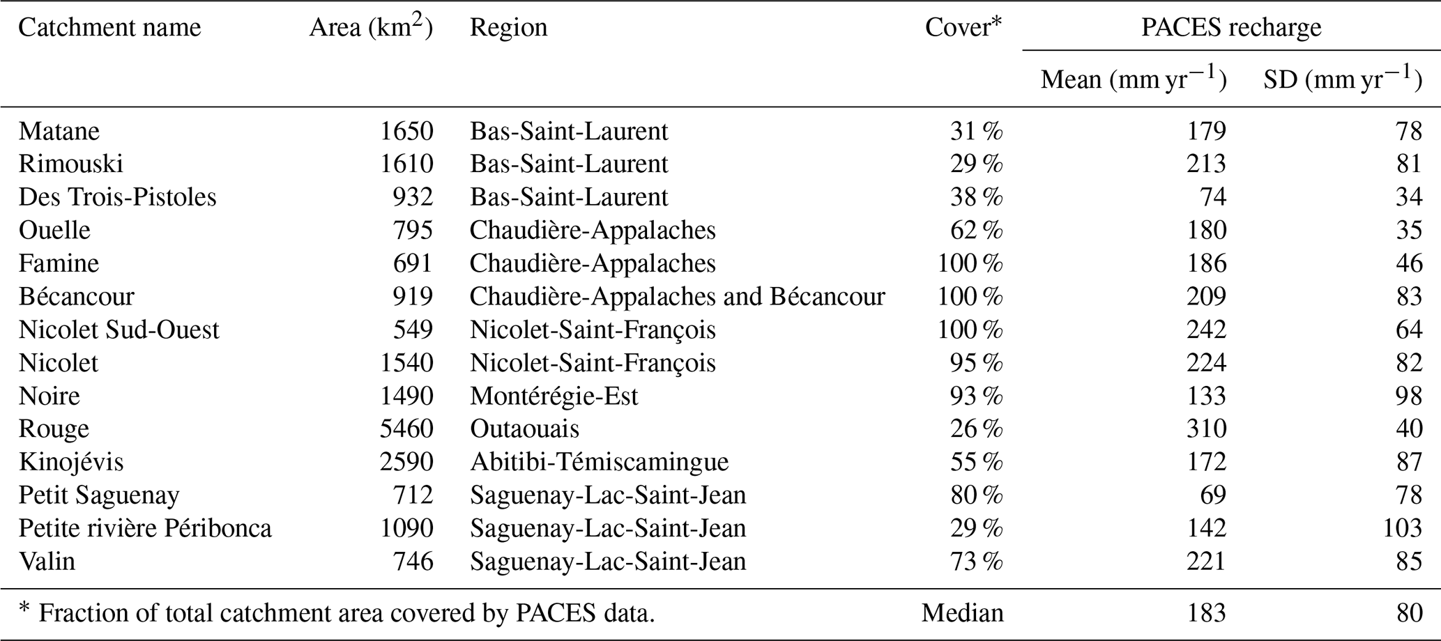
In 2008, the Government of Quebec initiated the “Projets d'acquisition de connaissances sur les eaux souterraines” (PACES; roughly translated as “groundwater knowledge acquisition projects”) (Carrier et al., 2013; Cloutier et al., 2013, 2015; Comeau et al., 2013; Larocque et al., 2013, 2015; Rouleau et al., 2013; Buffin-Bélanger et al., 2015; Lefebvre et al., 2015), aimed at enhancing understanding of the groundwater resources availability in Southern Quebec area. In addition to PACES, numerous studies conducted across the region have estimated groundwater recharge rates, which vary from 50 to over 500 mm yr⁻¹ depending on the location and years studied (Croteau et al., 2010; Chemingui et al., 2015; Larocque et al., 2019; Dubois et al., 2021; Boumaiza et al., 2022).

Of the 34 catchments in this study, fourteen were entirely or partially covered by the PACES project. Table 2 lists these catchments, detailing their areas, associated PACES region reports, the percentage of each catchment's area covered by PACES, and the mean and standard deviation of groundwater recharge for the areas covered.

Table 2 PACES data coverage and groundwater recharge statistics for covered catchments.

2.3 Hydrological modelling

2.3.1 WaSiM model

In this study, we employed WaSiM for hydrological modeling (Schulla, 2021). Hydrological processes were analyzed through three specific configurations: BL (baseline), which serves as the standard comparison model; GW (physical groundwater model), which incorporates detailed groundwater dynamics; and GW-RC (physical groundwater model with constrained recharge), which further refines the groundwater variables by incorporating constrained recharge calibrations. Detailed descriptions of these configurations can be found in Sect. 2.4 of this study.

WaSiM consists of two versions: WaSiM version I, originally developed using the Topmodel approach for simulating subsurface flows based on variable saturation areas, and WaSiM version II, an extended version with the process-oriented Richards approach. The Richards version, which considers hydraulic head gradients and detailed soil physical properties (pF-curve, k(u) function), was selected for this study due to its more physically based nature.

WaSiM follows a modular structure, composed of multiple sub-models that can be activated based on data availability and the specific research objectives. The model operates using a consistent time step, while internally employing flexible sub-time steps to optimize computational efficiency. It accommodates both regular and irregular raster grids, enabling the analysis of diverse spatial configurations. During each time step, the sub-models are sequentially processed across the entire model grid, enabling parallelization to aid computational optimization and facilitate faster model execution.

One of the key process modules within WaSiM is the unsaturated zone model, which plays a crucial role in calculating various hydrological variables such as surface runoff, groundwater recharge, interflow, and baseflow. Interflow refers to water moving laterally through the upper soil layers, contributing to streamflow, while baseflow is the portion of streamflow sustained by groundwater flow. These variables are essential for understanding the water balance and hydrological dynamics within the study area. Table 3 provides an overview of the hydrological model configuration used in this study.

Table 3 Overview of WaSiM characteristics and sub-models used in this study.

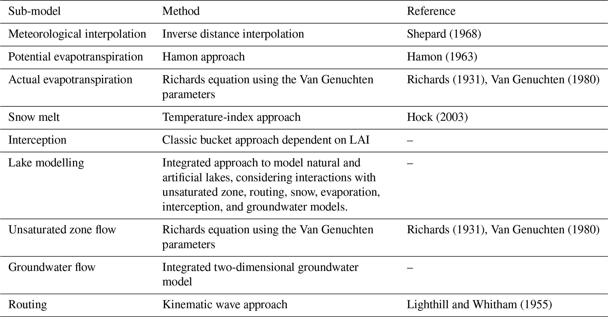
Meteorological data interpolation was an essential step in the hydrological modeling process. The chosen hydrological model, WaSiM, performed the interpolation of daily precipitation and temperature inputs between ERA5 points. For each simulation, the model creates grids that incorporate the interpolated meteorological values at the model's spatial resolution, effectively representing the climatic conditions for each individual pixel. The inverse distance weighting method was used as recommended by WaSiM model description report (Schulla, 2021).

2.3.2 Calibration parameters

Calibration of WaSiM involved the optimization of 17 parameters, selected in accordance with WaSiM documentation (Schulla, 2021), while the remaining parameters in the control file were set to their default values. Table 4 provides a detailed description of upper and lower limits set for calibrating the 17 parameters in WaSiM, with each parameter adjusted to two decimal places within the specified calibration range.

Table 4 Description of the parameters used for the calibration of WaSiM.

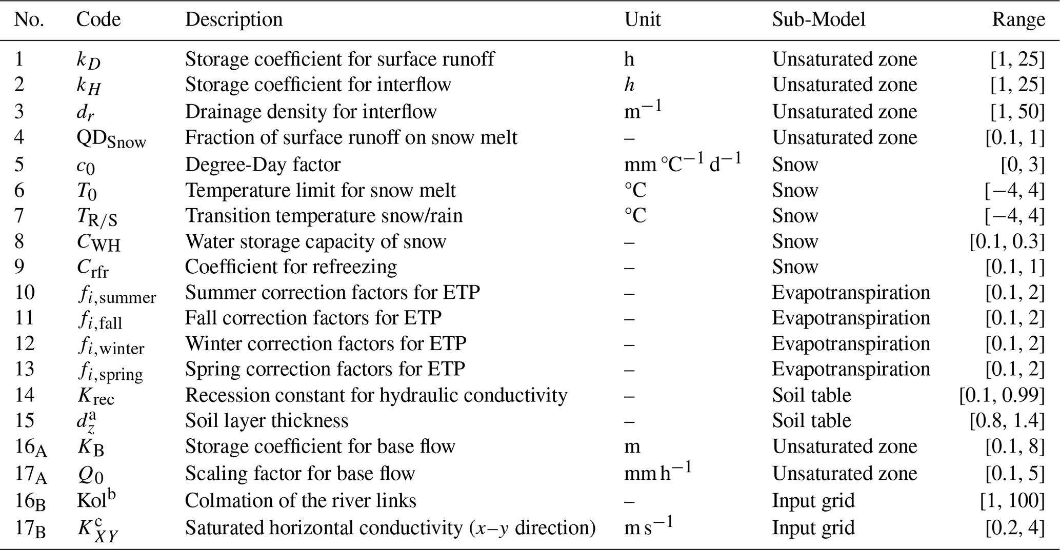
^a Calibration coefficient, ranging from 0.8 to 1.4, is applied to adjust the total soil depth, which is predetermined to be 8 meters for shallow, 14 m for normal, and 20 m for deep soil conditions. ^b Calibration coefficient, ranging from 0.8 to 1.4, is applied to adjust the colmation grid, which is predetermined to be $\mathrm{1}\times {\mathrm{10}}^{-\mathrm{6}}$. ^c A calibration coefficient, ranging from 0.2 to 4, is applied to adjust the saturated horizontal conductivity grid, which is predetermined to be $\mathrm{4}\times {\mathrm{10}}^{-\mathrm{5}}$ m s⁻¹.

For each model configuration (BL, GW, GW-RC), the full set of 17 parameters was recalibrated independently within the specified ranges. In the BL configuration, where the groundwater model is not activated and groundwater flow is computed using a conceptual approach within the unsaturated zone sub-model, parameters 16_A (K_B) and 17_A (Q₀) were the ones calibrated for baseflow representation, as these parameters are only relevant when the conceptual groundwater scheme is used. Groundwater flow is assessed using Eq. (1) (Schulla, 2021), which calculates baseflow as a function of several parameters including the scaling factor for baseflow (Q₀) and the recession constant for baseflow (K_B).

$$\begin{array}{}\text{(1)}& Q_{\mathrm{B}}=Q_{\mathrm{0}}\cdot K_{\mathrm{s}}\cdot e^{(h_{\mathrm{GW}}-h_{\mathrm{geo},\mathrm{0}})/K_{\mathrm{B}}},\end{array}$$

where Q_B is baseflow (m s⁻¹), Q₀ is a scaling factor for baseflow, K_s is the saturated hydraulic conductivity (m s⁻¹), h_GW is the groundwater table height (m), h_geo,0 is the geodetic altitude of the soil surface (m) and K_B is the recession constant for baseflow (m).

In the configurations used in GW and GW-RC, which activate groundwater model, parameters 16_A and 17_A are replaced by parameters 16_B and 17_B to obtain a more physically based representation of groundwater processes. Parameters 16_B and 17_B adjust values associated to two input grids that allow to account for the colmation of the river links and saturated horizontal conductivity. This distinction ensures a consistent number of calibrated parameters across all configurations, facilitating an unbiased comparison of model performance.

2.3.3 Model optimization

Parameters optimization was performed independently for each catchment through the dynamically dimensioned search algorithm (DDS; Tolson and Shoemaker, 2007), following the recommendation of Arsenault et al. (2014). This algorithm is specifically designed for efficiently calibrating complex hydrological models with a large parameter range given a finite computing budget. During optimization, it dynamically adapts its search strategy based on the number of evaluations performed and performance metrics. To manage computational demands effectively while ensuring thorough exploration of the parameter space, a two-phase calibration strategy was employed, albeit the approaches differ for the constrained groundwater configurations.

Initially, 1000 simulations were performed for each catchment at a broader spatial resolution (1000 m) using a broader range of values for each parameter (Table 4). This phase aimed to identify an approximation of the optimal values for each parameter. Subsequently, these values were used to initialize the second calibration step at a finer spatial resolution (250 m). This two-step approach was chosen based on preliminary testing on the Bonaventure and Matane catchments, which demonstrated that transferring optimized parameters from 1000 m resolution to 250 m required only minor refinements. Additional tests showed that increasing the number of simulations at 250 m resolution beyond 50 runs (e.g., 75 or 100) provided negligible improvements in model performance, making further computational expense unjustified. This sequential calibration strategy allows to refine the model's performance progressively. By first identifying a set of parameters that achieves reasonable model performance at a coarser scale, we then fine-tune the model at a higher resolution to enhance the spatial distribution of hydrological simulations.

The objective functions used vary by configuration: For BL and GW, the objective is to optimize the Kling-Gupta Efficiency (KGE, Kling et al., 2012), as discussed in Sect. 2.5.1. Conversely, the GW-RC configuration employs a modified objective function that seeks to optimize KGE and constrain groundwater recharge rates and variability. This approach is described in Sect. 2.4.3 and 2.5.2.

The study employed split-sample test (SST) framework for the parameter optimization assessment. This widely used approach involves dividing the available data into two sets: one for calibrating the model and the other for validating its performance on unseen time periods. The calibration period (2000–2009) and the validation period (1990–1999) were chosen based on the availability of comprehensive and reliable hydrological data. To minimize the impact of missing streamflow data, calibration and validation years were selected to ensure that most catchments had complete records. However, data gaps were noted for three catchments: Croche, Petit Saguenay, and Sainte-Marguerite Nord-Est. Specifically, Croche lacked data from 2001 to 2004, Petit Saguenay from 2000 to 2010, and Sainte-Marguerite Nord-Est from 1998 to 2010. To accommodate these gaps, adjustments were made to the calibration and validation periods for the affected catchments. The calibration periods were shortened to later years: 1995 to 1999 for Croche and Petit Saguenay, and 1992 to 1996 for Sainte-Marguerite Nord-Est. Correspondingly, the validation periods were adjusted to precede the missing data: 1991 to 1994 for Croche, 1986 to 1994 for Petit Saguenay, and 1986 to 1991 for Sainte-Marguerite Nord-Est. A five-year spin-up period was performed before each simulation to allow the model to reach a stable state, eliminating the influence of unstable initial conditions on the model's performance metrics.

2.4 Model configurations

The primary objective of this research is to examine how different model configurations influence the representation of hydrological processes. To ensure a consistent comparison of model configuration and calibration, we designed a modelling framework that allow to compare three configurations that incrementally incorporate more complex hydrological variables.

2.4.1 Baseline

The first configuration (BL), serving as baseline configuration, employs the standard calibration of the model without activating the groundwater module. This configuration is aligned with the traditional application of WaSiM, where the focus is predominantly on streamflow, and groundwater flow is modeled using Eq. (1) within the unsaturated zone sub-model. This configuration is comparable to what has been frequently adopted in numerous studies, providing a common basis for comparative analysis (Rössler et al., 2012; Förster et al., 2018; Markhali et al., 2022; Valencia Giraldo et al., 2023).

2.4.2 Physical groundwater module

The second configuration, GW (physical groundwater), marks a departure from the BL configuration by activating WaSiM's groundwater module. This adjustment allows for groundwater flow to be simulated within a designated sub-model, transitioning from a conceptual to a more physically based representation. In WaSiM, the groundwater model is coupled bi-directionally with the unsaturated zone, ensuring a dynamic exchange of water fluxes. The unsaturated zone module calculates fluxes between the unsaturated zone and the groundwater that act as the upper boundary condition for the groundwater model, while the groundwater module simulates lateral flow and adjusts the groundwater table, feeding back changes to the unsaturated zone as inflow or outflow. This configuration, used in numerous studies (Bormann and Elfert, 2010; Natkhin et al., 2012; Gädeke et al., 2014; Schäfer et al., 2023), is recommended by the WaSiM documentation for catchments where groundwater dynamics play a pivotal role in the hydrological cycle, particularly in lowland areas with extensive sediment layers.

2.4.3 Physical groundwater module and constrained recharge

For configuration GW-RC (physical groundwater and constrained recharge), we incorporate groundwater recharge into the calibration process to achieve a better representation of hydrological variables such as baseflow, interflow, and runoff. Importantly, GW-RC uses the same model structure as GW, with the goal of isolating the effect of adding groundwater recharge in calibration. By introducing recharge into the calibration, we restrict hyperplane exploration and ensure that the model's representation of the hydrological cycle is more accurately simulating groundwater recharge dynamics. This is particularly useful if model hydrological variables are an important input to another analysis or process, such as for better understanding groundwater movement and evolution under climate change for certain types of vegetation, for example.

GW-RC calibration was performed in two phases. First, we defined new parameter ranges for variables affecting baseflow (d_r, QD_Snow, K_rec, Kol, K_xy). We first conducted 200 evaluations at a spatial resolution of 1000 m, followed by 50 evaluations at 250 m using the objective function presented in Eq. (2). Essentially, the aim here is to constrain the parameter set to a single value that performs well overall and provides realistic internal variables. Similar approaches have been used in studies such as Duethmann et al. (2024), which underscores the benefits of integrating Landsat-derived land surface temperature (T_s) data into model calibration. Landsat, a series of Earth-observing satellites, provides crucial T_s data used in this study. By including satellite-derived T_s, the study demonstrated improvements in the model's ability to capture spatial anomalies and ecosystem stress responses, while maintaining streamflow accuracy, illustrating the advantages of multi-variable constraints in model calibration.

Following pre-calibration at both spatial resolutions, the resulting calibrated parameter sets were analyzed to define new parameter ranges for the calibration phase. This analysis involved adjusting the minimum and maximum values of parameters influencing baseflow (d_r, QD_Snow, K_rec, Kol, K_xy) by ±10 % to establish new calibration ranges.

In the second and most important calibration phase, the process continued with the adjusted parameter ranges, employing a less restrictive objective function (Eq. 3) to better accommodate uncertainties in the recharge data. This phase involved a comprehensive series of 1000 evaluations at 1000 m and 50 at 250 m resolutions. The modified objective function primarily emphasized the KGE while incorporating the standard deviation of recharge at a reduced influence of 4 %. This modification was crucial to allow the model flexibility to adapt the groundwater recharge rate according to the specific hydrological characteristics and precipitation patterns of each catchment. Given that the initial recharge rate of 250 mm yr⁻¹ was a preliminary estimate and not necessarily reflective of individual catchment conditions, this approach enabled a more tailored calibration.

A key justification for not applying the same constrained parameter range across all configurations is that BL and GW do not incorporate recharge in calibration. Their parameters optimization is based solely on streamflow, whereas GW-RC explicitly integrates recharge to constrain the parameters range.

Table 5 shows an overview of the three methods to ease comparisons between configurations.

Table 5 Summary of configurations.

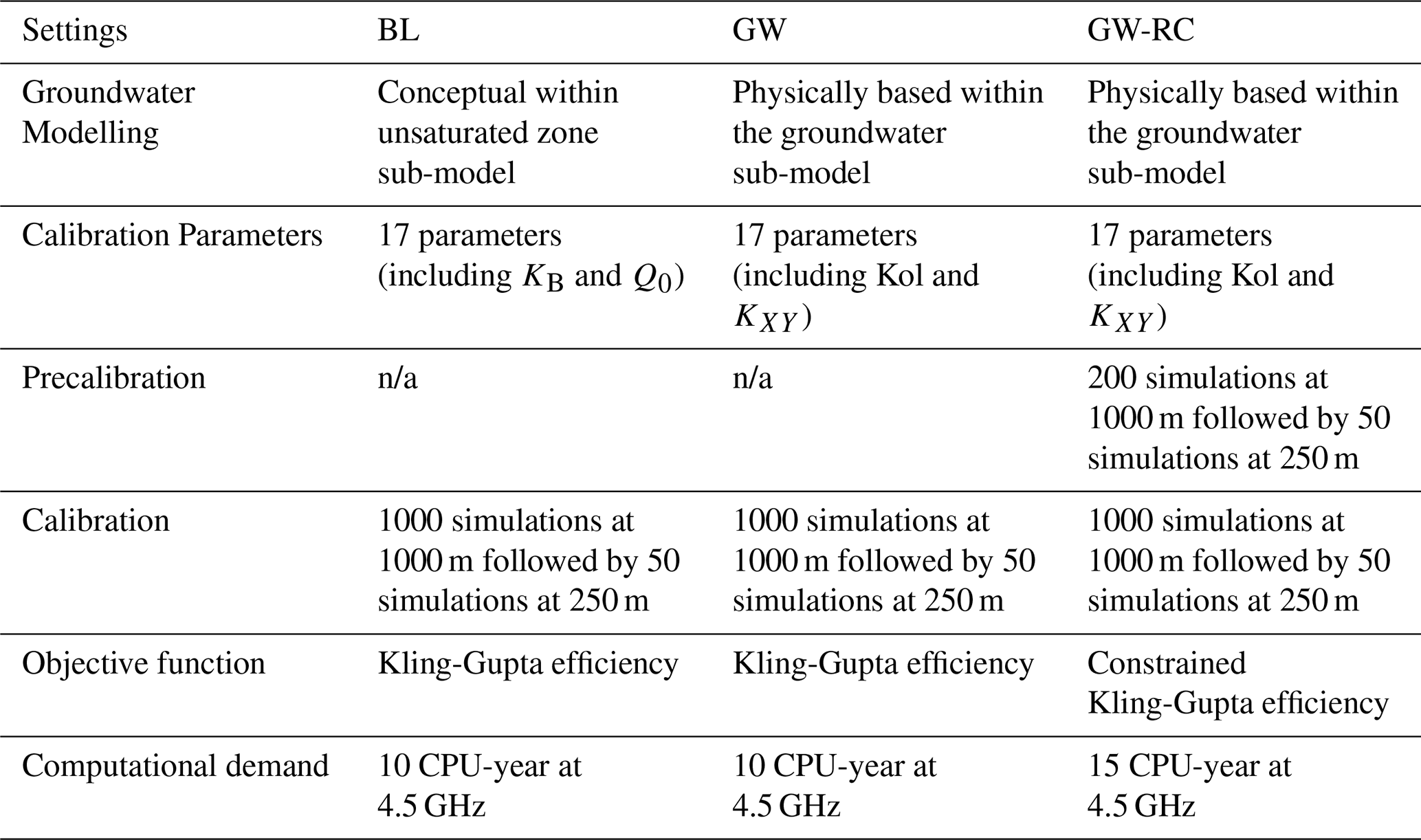
CPU-year: A CPU-year is the effort of a CPU running for one year. n/a: not applicable.

2.5 Performance assessments

The KGE (Kling et al., 2012) was chosen as the objective function to assess the model's performance during the calibration process of configurations BL and GW.

An arbitrary baseline groundwater recharge rate of 250 mm yr⁻¹ and a standard deviation of 80 mm yr⁻¹ have been established as representative benchmarks for the studied catchments. These values are based on PACES data and additional studies conducted in Quebec, as described in Sect. 2.2.5. The objective function for the pre-calibration of configuration GW-RC, outlined in Eq. (2), aims to balance KGE with these established recharge metrics. Specifically, the function assigns a weight of 70 % to KGE, 20 % to the annual recharge standard deviation, and 10 % to the mean annual recharge. This specific weighting was determined based on preliminary testing conducted on two test catchments, where various weight combinations were evaluated. The selected weights provided the best trade-off, ensuring that recharge estimates remained realistic while maintaining strong KGE values for streamflow. In particular, assigning 20 % to the recharge standard deviation and 10 % to the mean annual recharge allowed the model to better capture recharge variability without compromising overall streamflow performance. This objective function was designed to ensure both the quantity and variability of recharge were realistically modeled without sacrificing performance in terms of overall streamflow quality through the KGE.

The objective function employed in the pre-calibration of GW-RC configuration is formulated as follows:

$$\begin{array}{}\text{(2)}& \begin{array}{rl}\text{Precalibration function}& =\mathrm{1}-(\mathrm{0.7}\cdot \text{KGE}+\mathrm{0.2}\\ & \cdot ⌈{\mathit{\sigma }}_{r_{\mathrm{sim}}}-\mathrm{0.08}⌉+\mathrm{0.1}\\ & \cdot ⌈\stackrel{\mathrm{‾}}{r_{\mathrm{sim}}}-\mathrm{0.25}⌉),\end{array}\end{array}$$

where ${\mathit{\sigma }}_{r_{\mathrm{sim}}}$ is the simulated annual recharge standard deviation (m yr⁻¹), $\stackrel{\mathrm{‾}}{r_{\mathrm{sim}}}$ is the simulated mean annual recharge (m yr⁻¹) and KGE is the Kling-Gupta efficiency.

Groundwater recharge simulations were performed at the pixel level, ensuring detailed local representation. The simulated mean annual recharge reflects the average amount of recharge occurring annually across the entire catchment during the calibration period. Similarly, the simulated annual standard deviation quantifies the variability in annual recharge across all pixels within the catchment during the same period. Introducing pixel level standard deviation helps in curbing extreme values in groundwater recharge, thus stabilizing the simulation outputs. The mean annual recharge is employed to verify that the model accurately captures the overall recharge volume expected for the study area.

For the main calibration phase of the GW-RC configuration, the objective function is simplified to focus more intensively on streamflow accuracy:

$$\begin{array}{}\text{(3)}& \mathrm{\text{Calibration function}}=\mathrm{1}-(\mathrm{0.96}\cdot \text{KGE}+\mathrm{0.04}\cdot ⌈{\mathit{\sigma }}_{r_{\mathrm{sim}}}-\mathrm{0.08}⌉),\end{array}$$

where ${\mathit{\sigma }}_{r_{\mathrm{sim}}}$ is the annual recharge standard deviation (m yr⁻¹) and KGE is the Kling-Gupta efficiency.

2.6 Statistical analysis

To assess the performance of the hydrological model configurations, statistical analyses were conducted to compare calibration and validation performance across different configurations. The primary metric used was the KGE, which evaluates the accuracy of simulated streamflow against observed data. The performance metrics were analyzed for each configuration during both the calibration period (2000–2009) and validation period (1990–1999), ensuring robust evaluation across varying hydrological conditions.

All statistical comparisons were made using the Kruskal-Wallis test, a non-parametric method chosen due to its suitability for non-normally distributed data. This test was employed to detect significant differences in the performance and hydrological responses between the model configurations. Where significant differences were identified, multiple comparison post-hoc tests were conducted to ascertain the specific pairs of configurations that differed significantly.

Pearson's correlation coefficients were used to explore the influence of calibration parameters on hydrological variables. This statistical approach provided insights into how variations in parameter settings across different configurations could affect the representation of hydrological processes like surface runoff, interflow, and groundwater recharge.

3 Results

3.1 Calibration and validation performance

Throughout the calibration (2000–2009) and validation (1990–1999) periods, all configurations yielded KGE values above 0.5. Calibration and validation performances were very similar, with a deviation less than 5 %, demonstrating the robustness of the simulations. KGE values for all catchments and configurations, for both the calibration and validation periods, are presented in Table A1.

Figure 2 reveals a clear trend where catchments with high KGE values during calibration tend to maintain similar performance during validation. This consistency underpins the robustness of the configurations across different validation periods. During the validation period, median KGE values were higher for configurations BL (0.824) and GW (0.830) compared to GW-RC (0.770), demonstrating superior performance in the models without groundwater recharge constraints. However, GW-RC demonstrates more consistent KGE values between calibration and validation, suggesting it may offer more stability in model performance despite its slightly lower KGE scores.

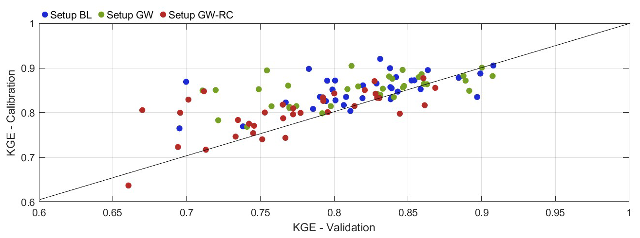
Figure 2 Comparison of Kling-Gupta Efficiency values between calibration and validation periods for three configurations. Each point represents a catchment, color-coded by configuration: Configuration BL (blue), Configuration GW (green), and Configuration GW-RC (red). The line represents a one-to-one relationship where calibration and validation KGE values are equal. Points below the line indicate better performance in the validation phase compared to calibration, while those above the line show a decline in performance from calibration to validation.

It is important to note that the KGE values for configuration GW-RC are slightly lower than those from configurations BL and GW, which is expected given the supplementary constraints imposed during calibration.

3.2 Hydrological variables analysis

This section delves into the simulated hydrological variables, examining their range and distribution across the various model configurations during the calibration and validation periods. The variables in focus include surface runoff, baseflow, interflow, groundwater recharge, and actual evapotranspiration (ETa).

Figure 3 illustrates the annual totals (means for groundwater level and soil moisture) for simulated hydrological variables for both calibration and validation periods and for all catchments. Notably, there is a consistency in the distribution of hydrological variables of each model configuration between the calibration and validation periods. This allows us to focus our detailed analysis solely on the validation period for conciseness.

A comparative assessment reveals distinct patterns in the simulated hydrological variables among the configurations. Specifically, configuration GW-RC simulates higher surface runoff and lower interflow, and infiltration compared to configurations BL and GW. Conversely, configuration BL is characterized by higher actual evapotranspiration, lower groundwater recharge, and a higher groundwater level. Configuration GW shares similarities with both configuration BL (in terms of runoff, interflow, and infiltration) and configuration GW-RC (regarding baseflow, groundwater recharge, actual evapotranspiration, and groundwater level).

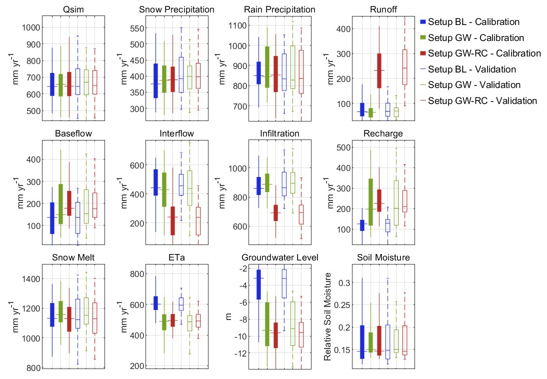
Figure 3 Boxplots illustrating annual totals (means for groundwater level and soil moisture) variability of model internal variables. These boxplots detail the variability of key hydrological variables modeled with the different configurations, for calibration and validation periods and for all catchments.

Figure 4 presents the proportional distribution of surface runoff, baseflow, interflow, and actual evapotranspiration for the three hydrological model configurations (BL, GW, and GW-RC). The charts effectively compare the relative contribution of each process to the total water cycle within the modeled catchments.

The figure highlights that configuration GW-RC simulates a notably higher proportion of surface runoff (21 %) and baseflow (17 %) with a lower proportion of interflow (20 %). Conversely, configuration BL has a higher proportion of actual evapotranspiration (47 %) and less baseflow (11 %). Finally, configuration GW has similarities with both BL (surface runoff and interflow) and GW-RC (baseflow and actual evapotranspiration) configurations. The factors influencing the differences between configurations are further analyzed in the discussion section.

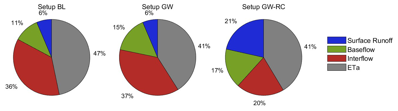
Figure 4 Proportional distributions of key hydrological variables for the BL, GW and GW-RC hydrological model configurations for the validation period (1990–1999).

Table 6 shows that the observed similarities in surface runoff and interflow between configurations BL and GW are substantiated by statistical significance in their mean groupings. Furthermore, the parallels drawn between configurations GW and GW-RC in terms of actual evapotranspiration and groundwater recharge are also supported by significant statistical evidence. However, the apparent similarity in baseflow between configurations GW and GW-RC does not hold statistical significance. This outcome is expected, as both GW and GW-RC employ the same groundwater module, with GW-RC differing only in its calibration approach. The observed variations in baseflow arise from the inclusion of recharge constraints in GW-RC. More broadly, the significant contrast in baseflow between BL and the other two configurations suggests that the choice of model configuration plays a primary role in determining baseflow dynamics rather than the specific calibration strategy applied.

Table 6 Statistical analysis of the differences in estimated hydrological variables from the three configurations BL, GW and GW-RC.

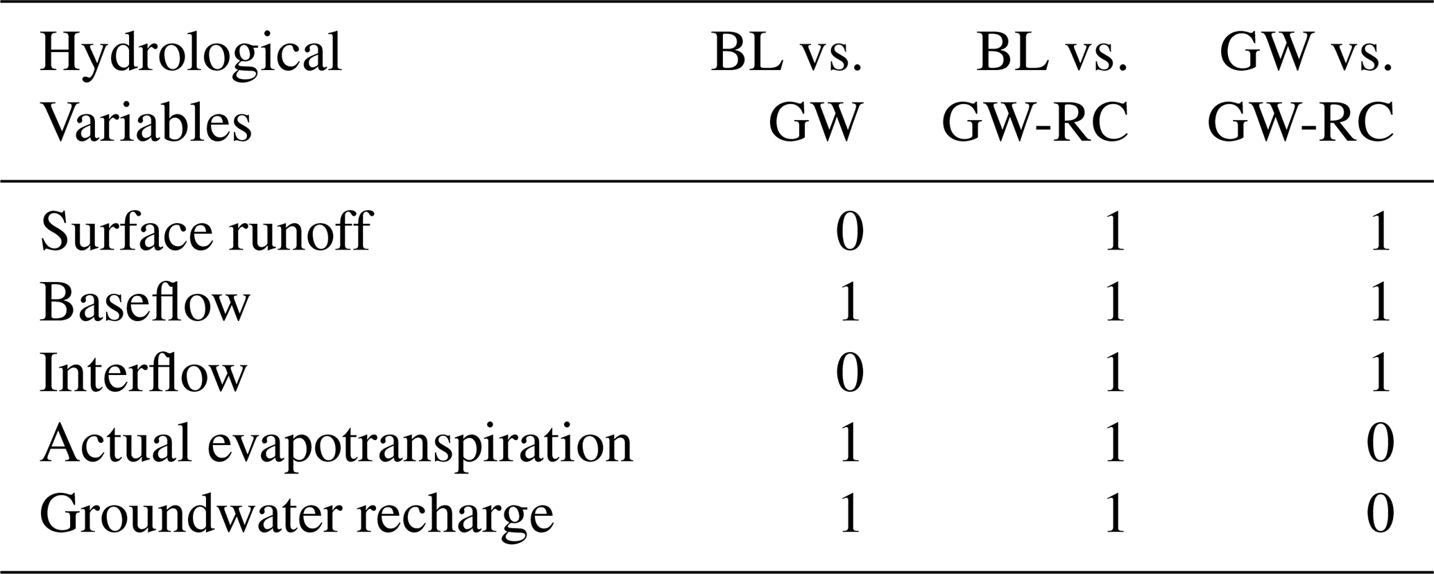
(Not Different = 0; Different = 1)

Figure 5 illustrates the annual totals distribution of key hydrological variables (surface runoff, baseflow, interflow, actual evapotranspiration, groundwater recharge, and precipitation) across 34 catchments for each model configuration (BL, GW, and GW-RC). The figure provides a comprehensive comparison of how each configuration partitions the water balance components for each catchment. Consistent trends in hydrological responses are observed across the catchments for each model configuration. For instance, configuration GW-RC shows higher surface runoff and baseflow, with lower interflow values compared to the other configurations indicating that calibration strategies and model complexity influence the distribution of water fluxes. In contrast, configuration BL consistently reports higher actual evapotranspiration (ETa) and lower groundwater recharge. Statistical comparisons indicated that baseflow, surface runoff and interflow dynamics of GW-RC configuration are significantly different compared to BL and GW configurations (Table 6).

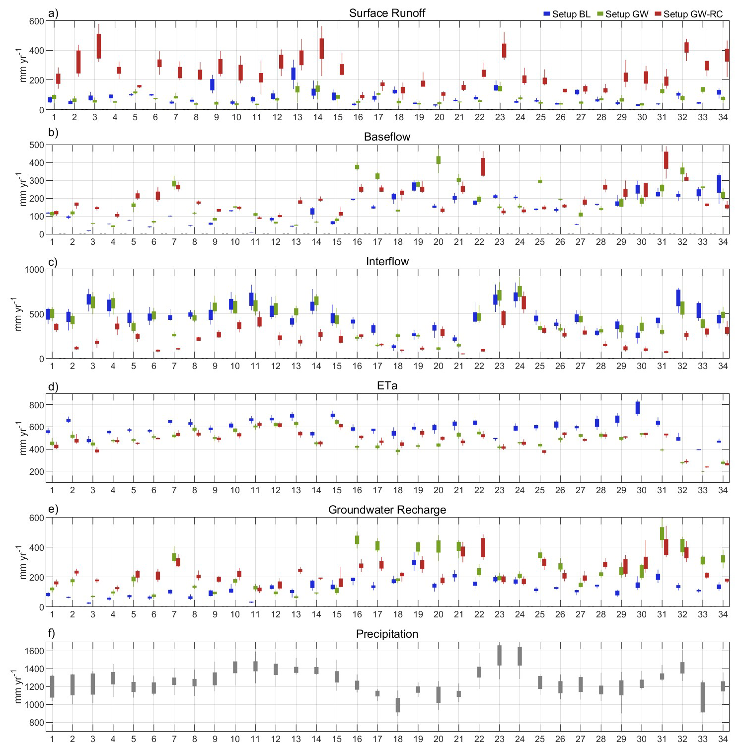
Figure 5 Boxplots of annual values for key hydrological variables predicted by WaSiM for the 34 catchments and three configurations for the validation period (1990–1999).

3.3 In-depth analysis of the Matane catchment

This section explores the temporal dynamics of streamflow and hydrological variables in the Matane catchment, which was selected as a representative example from the study's catchments. Figure 6 reveals consistent patterns in hydrological variable behavior across all configurations during both the calibration and validation periods. Consequently, the following discussions will focus primarily on the validation period. Generally, interflow is the major contributor to simulated streamflow in configurations BL and GW throughout the year. In contrast, configuration GW-RC is characterized by a significant increase in surface runoff during the seasonal high flow and high precipitation periods in the fall, while predominantly exhibiting interflow contributions during other times of the year.

Configuration GW-RC is also marked by higher levels of surface runoff and baseflow, but lower interflow compared to the other configurations. Configuration BL is distinguished by having the highest levels of annual actual evapotranspiration. Configuration GW aligns closely with configuration BL in terms of interflow, surface runoff, and baseflow, demonstrating similar hydrological dynamics between these two configurations.

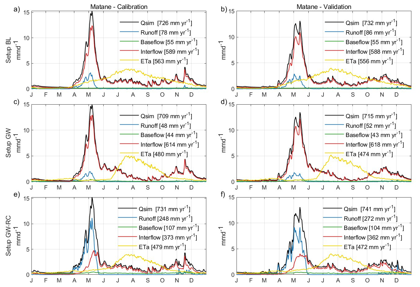
Figure 6 Detailed hydrological variable hydrograph for Matane catchment during both the calibration and validation phases and for the three configurations. Calibration results are shown in panels (a), (c), and (e) for Configurations BL, GW, and GW-RC, respectively, while validation results are depicted in panels (b), (d), and (f). These hydrographs demonstrate how baseflow, interflow and runoff contribute to total streamflow throughout the year, with noted annual totals provided for a comprehensive comparison.

Figure 7 reveals seasonal variations that correlate with hydrological responses to climatic conditions. Surface runoff and interflow differ significantly during periods of high flow, typically driven by snowmelt. Configurations BL and GW primarily attribute high flows to interflow, whereas configuration GW-RC reflects these peaks with increased surface runoff. Groundwater recharge in configuration BL exhibits more pronounced seasonal fluctuations compared to the patterns observed in configurations GW and GW-RC. Similarly, configuration BL maintains a consistent baseflow year-round, unlike configurations GW and GW-RC, which show seasonal baseflow variations. In terms of actual evapotranspiration, configuration BL consistently exhibits higher rates in the spring and fall, GW peaks during the summer, and GW-RC displays a pattern that blends characteristics of both BL and GW across different seasons.

Figure 7c illustrates the daily groundwater recharge in the Matane catchment for each configuration. A common seasonal pattern is evident across all configurations: recharge decreases in winter, rises significantly during snowmelt, and then exhibits marked variability throughout summer and autumn. Notably, configuration GW-RC shows a lower dynamic range during snowmelt compared to configurations BL and GW, which exhibit more pronounced peaks. Throughout the winter, summer, and autumn months, configuration GW-RC consistently shows higher recharge rates than the other configurations. The trends observed in the Matane catchment are also representative of the behaviors seen across all studied catchments.

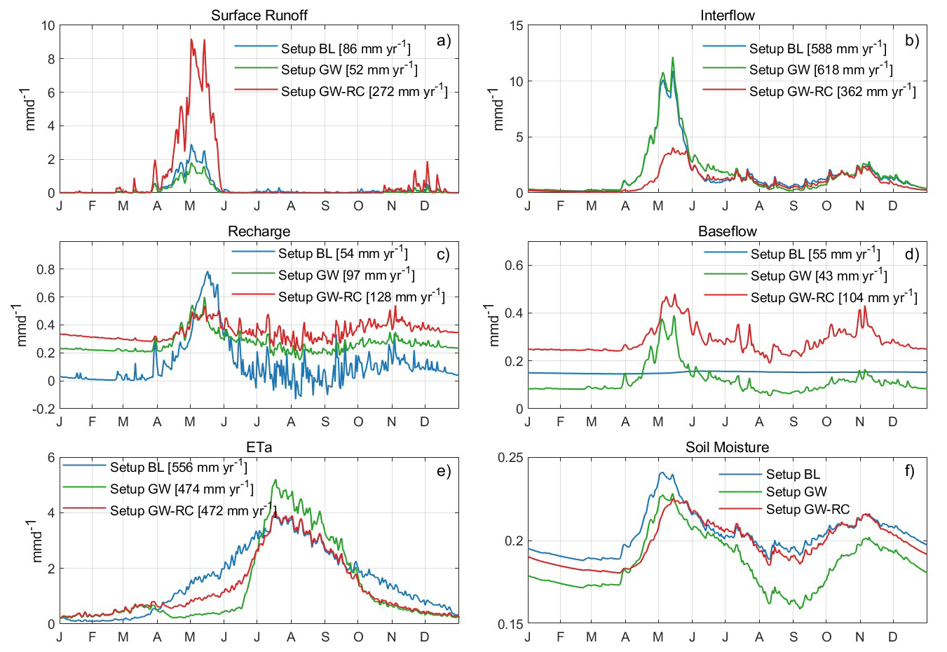
Figure 7 Seasonal distribution of hydrological variables in the Matane catchment for the validation period (1990–1999). This figure visualizes the annual distribution of key hydrological variables across the three configurations throughout the year.

4 Discussion

4.1 Performance against representation

This study aimed to analyze how varying model configurations affect the representation of hydrological variables estimated by WaSiM. Through the comparative analysis of three distinct calibration configurations, BL (baseline model), GW (activated groundwater simulation), and GW-RC (groundwater simulation and recharge calibration), this study provides insights into how internal hydrological processes are represented in a physically based model.

KGE values were consistently higher for the BL and GW configurations compared to GW-RC during both calibration and validation periods. Configuration GW-RC's modestly lower performance on KGE is reflective of its calibration not solely focusing on optimizing KGE but also in incorporating a broader suite of hydrological dynamics.

This finding aligns with prior research, which suggests that adding constraints to model parameters can often improve the representation of other hydrological processes, such as groundwater dynamics and soil moisture, albeit at the cost of lower validation performance. For instance, Yassin et al. (2017) emphasized that incorporating additional data, such as from the Gravity Recovery and Climate Experiment (GRACE), can lead to more comprehensive and physically realistic model. Similarly, Dembélé et al. (2020) showed that incorporating spatial patterns from satellite data significantly improve the model's representation of soil moisture and evapotranspiration. Similarly, Bouaziz et al. (2021) found substantial disparities in internal process representation among models calibrated to the same streamflow data, highlighting the limitations of relying solely on discharge data for model validation. Lastly, Pool et al. (2024) demonstrated that incorporating variables such as actual evapotranspiration and total water storage alongside discharge in model calibration can significantly enhance the simulation accuracy for these variables.

4.2 Hydrological variables analysis

Regarding the distribution of hydrological variables, configuration BL demonstrated the highest actual evapotranspiration rates, alongside the lowest groundwater recharge and baseflow. Conversely, GW-RC was noted for the highest surface runoff and the lowest interflow. Configuration GW exhibited characteristics that were intermediate between the other two configurations. It resembled BL in terms of interflow and surface runoff but aligned more closely with GW-RC for groundwater recharge, actual evapotranspiration, and baseflow.

As shown in Fig. C1, baseflow is closely correlated ($r=-\mathrm{0.875}$) with the drainage density parameter (scaling parameter for interflow) for configurations GW and GW-RC. The constrained parameter range in configuration GW-RC explains the minor differences in baseflow rates observed between these configurations. In contrast, the baseflow in configuration BL is significantly correlated (r=0.715) with the scaling factor for baseflow. The differences in groundwater recharge and baseflow across the configurations can be primarily attributed to the activation of the groundwater flow sub-model. In WaSiM, the simulation of groundwater processes can either follow a more conceptual or physically based pathway. Our results indicated that GW and GW-RC, which incorporate more complex mechanisms between groundwater and surface processes, lead to more dynamic and possibly more accurate representations of baseflow and recharge dynamics.

The disparities in interflow for configuration GW-RC are primarily due to the restricted calibration of the drainage density parameter. A strong correlation (r=0.801) between interflow rates and the parameter value highlights how constraining groundwater recharge during calibration can influence other hydrological variables, such as interflow. Variations in surface runoff for configuration GW-RC are linked to calibration restrictions on the “QD_Snow” parameter, which represents the fraction of surface runoff from snowmelt. A strong correlation (r=0.899) between this parameter and surface runoff rates indicates that it has a significant influence on this hydrological variable. Also, configuration GW-RC showed the highest value for “QD_Snow” parameter and the lowest value for the drainage density parameter consequently leading to the highest surface runoff and lowest interflow rates. This observation indicates that interflow is a flexible variable within the model, with configurations BL and GW appearing to prioritize it over surface runoff and baseflow. This prioritization allows the optimization algorithm greater latitude to enhance performance metrics like KGE and more accurately reproduce observed streamflow patterns. Conversely, configuration GW-RC, constrained by groundwater recharge, tends to prioritize baseflow and surface runoff. While this approach may reduce the model's flexibility in mirroring observed streamflow, it enhances the precision with which other hydrological processes are represented as detailed in Sect. 4.3. The same trend was found for the Matane catchment, underlining the broader applicability of these findings across different geographical contexts. Such a representation offers essential information that can be pivotal for water management strategies.

Moreover, configuration GW-RC also exhibited lower values of k_h (storage coefficient for interflow), higher values of K_rec (recession constant for hydraulic conductivity), lower correction factors for PET in summer, and higher correction factors for PET in winter compared to the other two configurations. These differences indicate that adding groundwater recharge constraints during calibration can influence parameter values in sub-models that are seemingly unrelated to groundwater processes, such as evapotranspiration. This suggests that the recharge constraint propagates through the model structure, affecting multiple hydrological components. A complete list of calibrated parameter values for each catchment and configuration is provided in Appendix D.

4.3 Pinpointing the optimal model configuration

The differences in surface runoff during the snowmelt season across configurations can be largely attributed to the parameter QD_Snow. WaSiM employs a singular parameter (QD_Snow) to account for surface runoff from snowmelt. This parameter is calibrated between 0 and 1, and its precise setting critically influences the model's surface runoff predictions.

Analysis of Fig. 6 reveals that configurations BL and GW exhibit lower surface runoff from snowmelt, where melted snow predominantly percolates into the soil, contributing to interflow rather than surface runoff. This behavior is unexpected because, in fully frozen soil conditions, significant surface runoff is typically anticipated due to reduced infiltration.

Conversely, configuration GW-RC, which integrates groundwater recharge into the calibration process, follows a more typical hydrological pattern. Higher surface runoff is observed at the onset of snowmelt, gradually decreasing as infiltration and interflow increase when the soil thaws. This progression aligns with the expected hydrological responses in frozen terrains, illustrating how the inclusion of groundwater recharge can improve the model's simulation of seasonal transitions. This trend of higher surface runoff during snowmelt was observed consistently across all catchments in the study, with detailed figures provided in the Supplement (Figs. S1 to S32). Configuration GW-RC showed increased surface runoff during the snowmelt period compared to the other configurations. However, for 11 out of the 34 catchments, the surface runoff results were notably elevated. Figure B1 illustrates an example where nearly all of the spring discharge was attributed to surface runoff, suggesting that the value assigned to the QD_Snow parameter, when set too close to 1, may lead to an overestimation of runoff. Careful calibration of this parameter is essential to avoid misrepresentations in the hydrological processes.

The analysis of groundwater recharge, as detailed in Sect. 3.4, reveals significant differences in seasonal dynamics and spatial distribution among the configurations. Notably, GW-RC displays less dynamic recharge rates during the snowmelt period compared to configurations BL and GW. This is indicative of a distinct interplay between surface runoff and infiltration processes within configuration GW-RC, where higher surface runoff during the spring results in reduced infiltration. Additionally, GW-RC exhibits higher recharge rates during summer, fall, and winter, with a peak in fall.

The spatial analysis of groundwater recharge across the catchments revealed key differences between the model configurations. Configuration BL struggled to simulate recharge rates exceeding 250 mm yr⁻¹, despite such values being common in the study area. However, it performed well in catchments with low recharge values, consistently producing lower recharge estimates compared to GW and GW-RC.

For configurations GW and GW-RC, groundwater recharge rates were influenced by catchment size and total precipitation. Larger catchments with higher precipitation exhibited greater recharge, while smaller, drier catchments showed lower recharge rates. This relationship indicates that these configurations better capture broad spatial trends in groundwater recharge compared to configuration BL, which showed less sensitivity to variations in precipitation and catchment size. Furthermore, GW and GW-RC displayed similar spatial patterns. Configuration GW exhibited the highest variability between catchments, whereas GW-RC produced estimates of average annual recharge that were more consistent with PACES data across most catchments. Future studies should further investigate how spatial characteristics of catchments affect the overall dynamics of hydrological variables in this context.

Supporting these observations, Chemingui et al. (2015) found the average recharge rates across different seasons at three locations in the “des Anglais” catchment. The numbers retrieve in their work closely align with those simulated by the GW-RC configuration: winter (58 vs. 50 mm), spring (58 vs. 54 mm), summer (92 vs. 60 mm), and fall (52 vs. 72 mm).

Furthermore, Rivard et al. (2014) utilized the HELP infiltration model to simulate recharge for a catchment in Eastern Canada, reporting average recharge rates of 67 mm in winter, 62 mm in spring, 27 mm in summer, and 76 mm in fall. These findings align with our results from configuration GW-RC, which also show peak recharge occurring in fall rather than in spring, differentiating it from the other configurations. Configuration GW aligns less precisely with these specific seasonal patterns, with a peak recharge in spring, but still outperforms BL in terms of matching the documented recharge rates from PACES.

Recharge rates from GW-RC compare favorably with observed seasonal fluctuations in the literature. Overall, GW-RC's alignment with empirical data and its ability to simulate hydrological processes more accurately make it a preferable model configuration for studying and predicting hydrological dynamics under varied climatic conditions.

In this study, the GW-RC configuration demonstrated that assigning a minor weight to recharge in the objective function can significantly enhance WaSiM's capability to represent hydrological variables accurately, even with non-exact prior recharge data. This approach underscores, again, the potential of leveraging prior information to refine model outputs, suggesting that even a modest emphasis on recharge within the calibration framework can lead to substantial improvements in model realism. This finding is particularly noteworthy as it implies that effective model calibration does not necessarily require precise initial recharge estimates if the calibration process is appropriately managed. It also points to the broader applicability of using informed yet flexible calibration strategies to improve hydrological models under varied conditions, highlighting a path forward for enhancing model accuracy with limited prior data.

4.4 Practical implications, general applicability and limitations

This research has practical applications beyond hydrological modeling. Integrating groundwater recharge into model calibration, as demonstrated in the GW-RC configuration, offers a more comprehensive approach to representing key hydrological variables. This approach is particularly valuable for improving predictions of water resources under varying climate conditions, as it enhances the accuracy of inputs critical to models of forest growth (Ford et al., 2011; Grant et al., 2013). As climate change continues to alter hydrological dynamics, the reliance on physically based models becomes crucial. These models are favored over conceptual ones or even machine learning based models because they can be adapted more readily to varying conditions, ensuring more robust predictions under climate change scenarios. For example, a strong recent trend is the use of deep learning architectures in hydrological modelling (Kratzert et al., 2018, 2019; Arsenault et al., 2023). These models simulate streamflow with generally better accuracy than traditional hydrological models, but they lack any mechanism to investigate internal and intermediate hydrological variables. Such adaptability is also critical for effective water resource management and mitigation of climate impacts (Wilby, 2005; Ludwig et al., 2009; Poulin et al., 2011). By improving the representation of hydrological processes, the GW-RC configuration may enhance the model's ability to simulate hydrological responses under changing climatic conditions. This is especially important given the non-stationarity of climate, where historical hydrological relationships no longer hold under future conditions. In this context, calibrating models using physically meaningful constraints, such as groundwater recharge, may improve their ability to capture shifting hydrological patterns and enhance confidence in assessments of climate change impacts on hydrological variables.

This research emphasizes the need to calibrate hydrological models using not only streamflow but also other variables such as groundwater recharge. This approach aligns with findings from other studies such as Yassin et al. (2017) and Dembélé et al. (2020), which advocate for multi-objective calibrations that enhance model reliability across different hydrological variables. By integrating measurements from diverse sources such as satellite data and in-situ measurements, models can avoid the pitfalls of calibration based solely on streamflow, which might not capture the full spectrum of watershed dynamics. Bouaziz et al. (2021) further illustrate this point by showing that hydrological models calibrated solely on streamflow can produce differing results when validated against other hydrological variables. This highlights the risk of equifinality, where different parameter sets yield similar streamflow outputs but diverge for other hydrological processes. Without proper constraints, such as incorporating groundwater recharge into calibration, models may generate realistic streamflow simulations while misrepresenting key internal processes. This issue is evident in configurations BL and GW, which fail to accurately capture certain underlying hydrological dynamics.

The methodology developed in this study has broad applicability beyond the specific context of Southern Québec. This approach can be valuable in a variety of geographic regions and hydrological settings, given similar contexts of equifinality (i.e. more processes and parameters than the data can support). Moreover, this multi-variable calibration method can enhance the accuracy of other distributed hydrological models by improving the representation of groundwater recharge related processes. Similar calibration techniques using remote-sensing data have been applied successfully in different settings, demonstrating that incorporating additional hydrological variables in calibration improves model performance.

Nevertheless, it is crucial to address the limitations of this study. The models' performance in replicating hydrological processes like soil frost impacts and its implications on runoff and recharge remain unknown. Future studies would benefit from incorporating field measurements alongside a broader range of climatic and hydrological conditions. Expanding the research to include different geographic regions with similar soil and climate characteristics could significantly enhance the validation and applicability of the findings.

Additionally, the selected catchments in this study range from 525 to 6840 km², which may limit the generalizability of the findings to catchments outside this size range. Future research could investigate smaller or larger catchments to determine whether the observed trends and calibration impacts remain consistent across different watershed scales.

Furthermore, the choice of objective function presents another limitation. This study primarily relied on the Kling-Gupta Efficiency (KGE) for streamflow calibration. However, alternative metrics such as SPAtial EFficiency (SPAEF) (Koch et al., 2018) could enable a more comprehensive evaluation of multiple hydrological components when using distributed hydrological models. The lack of sufficient spatially distributed observations prevented the application of SPAEF in this study, but future research could explore its use, particularly in conjunction with remote sensing data to better assess the spatial coherence of hydrological variables.

Moreover, the uncertainty inherent in modeling, especially with configurations that involve complex interactions of multiple variables, poses a continuous challenge. The study's reliance on specific data sets like PACES also introduces potential biases that could influence the generalizability of the findings. The two-step calibration adopted for GW-RC, necessitated by the absence of high-quality, spatially distributed recharge observations, limits the extent to which a fully direct comparison with GW can be achieved. Future work with access to such datasets could implement a single-step calibration using both streamflow and recharge, enabling a more controlled assessment of the effects of internal recharge constraints. It's essential for future research to explore these limitations, perhaps by expanding the range of observational data used for model validation.

In terms of practical implementations and further research, continuing to refine the calibration of hydrological models to include diverse hydrological variables can enhance their utility in real-world applications. Such efforts will help in developing more accurate flood forecasting models, improving water resource management strategies, and crafting more effective climate adaptation measures for forest, agricultural and anthropogenic ecosystems. This study advances calibration techniques in hydrological modeling, but further work is needed to develop universally reliable models.

5 Conclusion

This study examined the nuances of hydrological modeling under different calibration settings using WaSiM model across 34 catchments classified under climate zones Dfb and Dfc in Eastern North America. By implementing three distinct model configurations, BL (baseline model), GW (physical groundwater model), and GW-RC (physical groundwater and recharge calibration model), this research has demonstrated that incorporating groundwater recharge alongside streamflow during calibration process leads to a representation of hydrological processes that better aligns with expected system behavior.

The results indicate that the GW-RC configuration, enhanced with groundwater recharge calibration, aligns more closely with estimated groundwater recharge rates, thereby providing a more precise representation of groundwater behaviour both spatially and seasonally. The study also underscores the importance of extending calibration beyond traditional streamflow metrics to include other hydrological variables like groundwater recharge. This approach helps to mitigate the risks of equifinality.

Given the successful application of these methodologies within Eastern North American catchments, it presents an intriguing premise for their applicability to other geographical areas with similar hydrological contexts. Further research could explore how these calibration techniques perform under different hydrological conditions, potentially broadening our understanding of these relationships.

Appendix A

Table A1 Kling-Gupta efficiency values across studied catchments during calibration and validation periods, for the three calibrations configurations. Each row corresponds to a specific catchment, identified by its basin number.

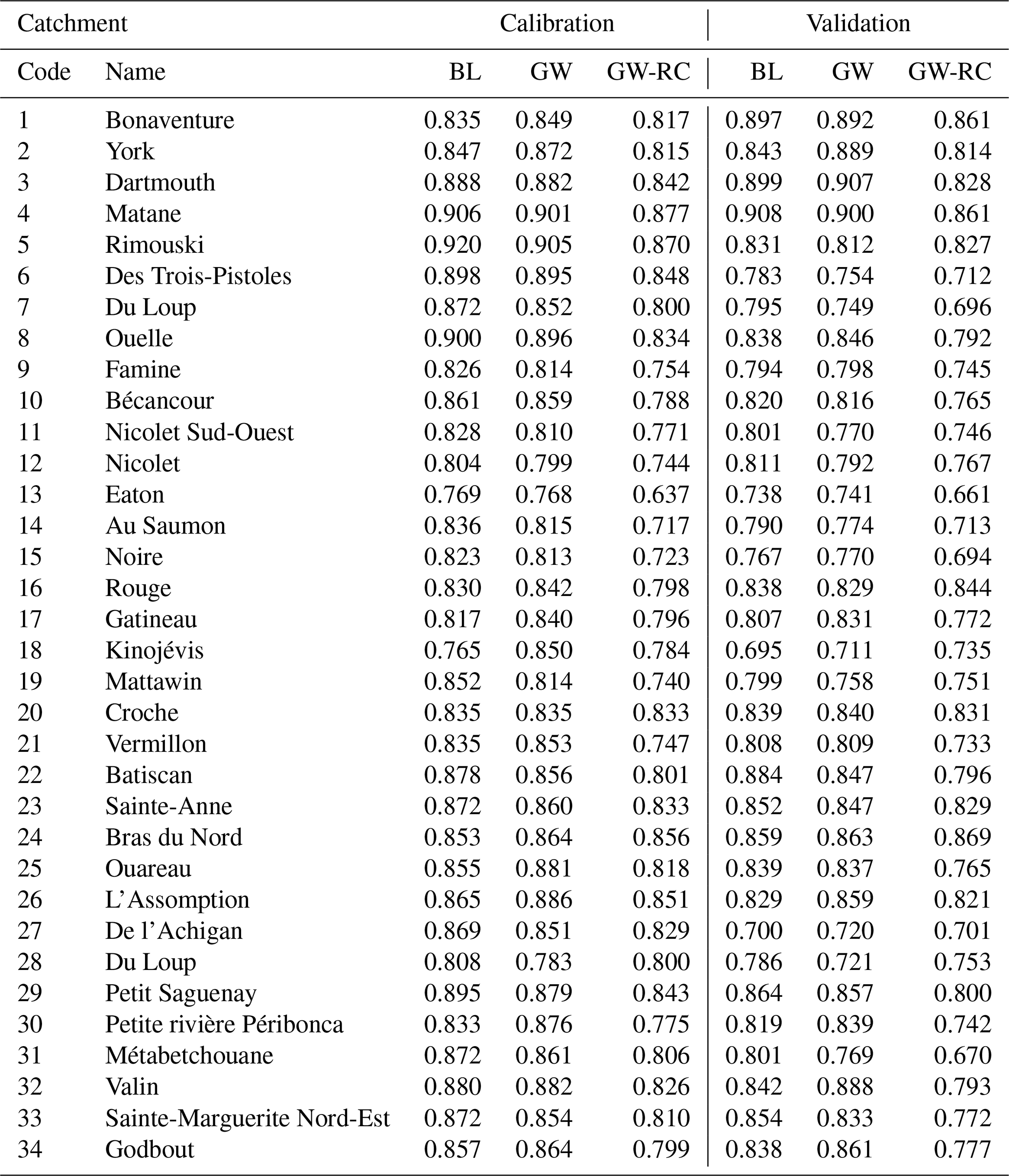
Table A2 Multiple streamflow metrics values during calibration (2000–2009) and validation (1990–1999) periods, for the three configurations.

Appendix B

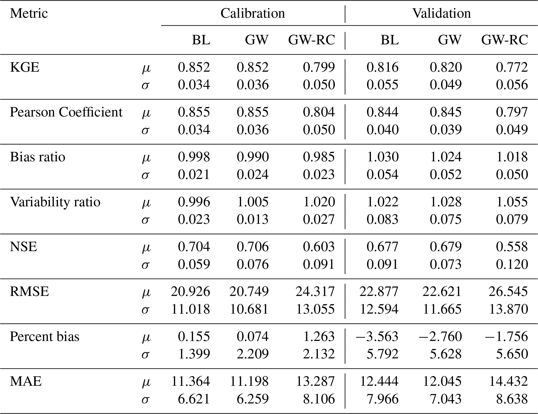
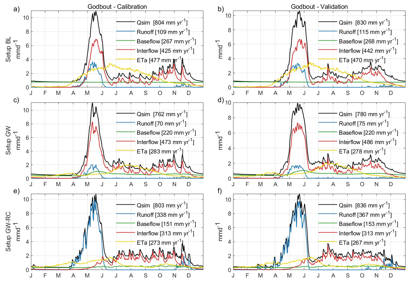
Figure B1 Detailed hydrological variable hydrograph for Godbout catchment during both the calibration and validation phases and for the three configurations. Calibration results are shown in panels (a), (c), and (e) for Configurations BL, GW, and GW-RC, respectively, while validation results are depicted in panels (b), (d), and (f). These hydrographs demonstrate how baseflow, interflow and runoff contribute to total streamflow throughout the year, with noted annual totals provided for a comprehensive comparison.

Appendix C

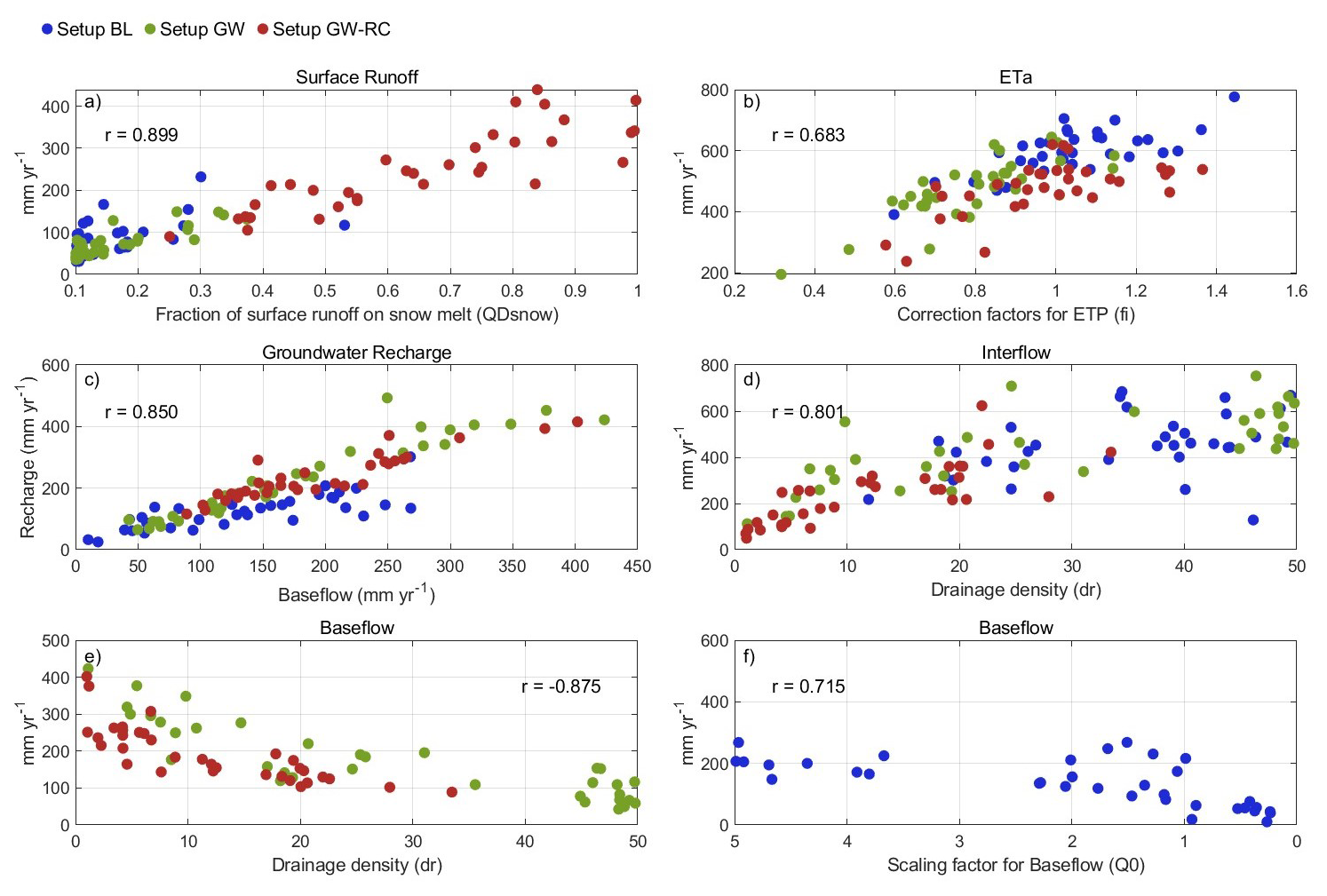
Figure C1 Correlations between key hydrological variables and calibration parameters for three model configurations.

Appendix D

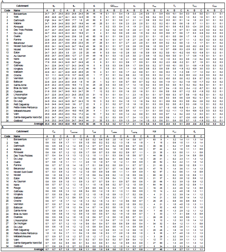
Table D1 Final calibrated parameter values for all catchments across each model configuration (BL, GW, GW-RC).