the Creative Commons Attribution 4.0 License.
the Creative Commons Attribution 4.0 License.
 | 19 Nov 2025
Data derived reservoir operations simulated in a global hydrologic model
Edwin H. Sutanudjaja
Marc Bierkens
Niko Wanders
Globally, there are over 24 000 storage structures (e.g. dams and reservoirs) that contribute over 7000 km3 of storage, yet most reservoir data is not openly accessible. As a result, many studies rely on generalized assumptions about reservoir storage dynamics to create generalized operational policies. With the creation of remotely sensed reservoir storage datasets such as RealSat and GloLakes and localized datasets such as ResOpsUS for the contiguous United States, and the Mekong Data Monitor for the Mekong River basin, the inference of reservoir operations using data derived techniques has become much more ubiquitous for regional studies. Yet to our knowledge, there has been no global application of data-derived methods due to data limitations and model complexities. Our analysis aims to fills this gap by providing a workflow for implementing data derived reservoir operations in large scale hydrologic models. This methodology uses global satellite altimetry data from GloLakes, a parameterization methodology developed by Turner et al. (2021), and a random forest model to extrapolate operational bounds. Our results demonstrate that our random forest algorithm can capture storage dynamics and that the associated errors are propagated from the type of data used. Additionally, we observe that deriving operational bounds from historical reservoir time series only directly impacts streamflow directly downstream of dams and has minimal impacts at the basin outlets. We do, however, observe that the data-derived methodology increases the accuracy of simulated global reservoir storage when compared to remotely sensed and observed storage observations. These derived storages are much lower than in generic operation schemes which suggests that current operational schemes are overestimating the amount of reservoir storage and potentially overestimating water availability. We also evaluated the sensitivity of our modelling framework to different downstream operating areas (i.e. 0 to 1100 km) and found that there were slight improvements when including downstream demands. Ultimately, our workflow allows global hydrologic models to capitalize on recent data acquisition by remote sensing to provide more accurate reservoir storage and global water security.
- Article
(9427 KB) - Full-text XML
- BibTeX
- EndNote


Across the globe, there are over 24 000 reservoirs that regulate 63 % of all global rivers (Hou et al., 2024), contain 61 % of the global seasonal variability in water storage (Cooley et al., 2021), and greatly decrease river connectivity (Grill et al., 2019; Belletti et al., 2020). With this loss of river connectivity comes a large amount of water storage (over 8 000 000 m3 (Lehner et al., 2011)) that provides water for a variety of main purposes, ranging from water supply and irrigation to hydropower and flood control. These storage structures also decrease streamflow variability with heightened effects during extreme flows (Salwey et al., 2023; Zajac et al., 2017; Chalise et al., 2021). With projected increases in global cropland (up to 1244 MHa) and over 90 % of the world's population living within 10 km of readily available surface water (Kummu et al., 2011; Potapov et al., 2021), the importance of reservoirs for flood control, irrigation, and water supply is large as the majority of society is dependent on reservoirs for a variety of uses (Di Baldassarre et al., 2018). Therefore, having an accurate depiction of reservoir storage at the global scale in observations and models is crucial to evaluating both historical and projected water availability.
Global reservoir storage capacity increased over the past 40 years as dams were built to support a variety of main uses (Lehner et al., 2011; Haddeland et al., 2006; Li et al., 2020; Wisser et al., 2013). This increase in storage capacity does not necessarily correlate with an increase in storage as many regions (primarily arid basins such as southeastern Australia, southwestern US, and eastern Brazil) have observed decreases in total reservoir storage (Steyaert and Condon, 2024; Li et al., 2020) due in part to increased domestic water demand resulting from population growth and decreased storage capacities from sedimentation (Simeone et al., 2024; Li et al., 2020; Wang et al., 2024; Wisser et al., 2013). This regionality is especially important as remote sensing observations show that most global reservoirs (more than 50 %) have not filled between 2010–2022, with many reservoirs in the Southern Hemisphere observing strong declines (Yao et al., 2023; Wang et al., 2024; Li et al., 2023). Ultimately, the regional differences in reservoir storage, the lack of observed filling, and the impact of sedimentation and water demand on storage levels are not well captured in generic operations due to simplified calculations that do not assimilate information derived from observed storage values.
This lack of accurate representation is due to the generic assumptions needed in reservoir operations (e.g. Meigh et al., 1999; Döll et al., 2003; Pietroniro et al., 2007; Rost et al., 2008) that use storage capacities (usually derived) from static datasets such as the Global Reservoirs and Dams Dataset (GRanD) (Lehner et al., 2011) or the World Registry of Dams accessible from the International Commission of Large Dams (ICOLD; https://www.icold-cigb.org, last access: 5 June 2024) and/or surface area to calculate a water balance in the reservoir at each time step. Any “excess” water above the storage capacity is then released downstream. These methodologies are more readily incorporated into large-scale hydrologic models, such as WaterGAP (Döll et al., 2009) and PCR-GLOBWB 2 (Sutanudjaja et al., 2018) due to their limited data requirements. Their main critiques lie in the assumption that reservoirs are usually filled to their maximum capacity, which overestimates the amount of storage (Steyaert and Condon, 2024; Salwey et al., 2023), and that they lack the incorporation of different operational policies. Additionally, they are limited by the availability of the static reservoir maps, and as a result, many only include the 6000 largest reservoir structures described in GRanD Lehner et al. (2011) even though more recent mapping by Wang et al. (2022) has shown there are over 24 000 reservoir structures. More recent advances by Salwey et al. (2023) and Brunner and Naveau (2023) focus on utilizing water balance methods to back-calculate transient reservoir characteristics from openly available data such as regional streamflow. These methodologies show promise regionally but have not yet been scaled to global applications nor implemented in global hydrologic models in part due to the lack of calibration data (Hosseini-Moghari and Döll, 2025).
More complex models of reservoir operations pushed for the inclusion of water demand and main use as a driving factor for reservoir releases in order to better represent reservoir operations. These policies included demand and policy changes based on main reservoir use (pioneered by Hanasaki et al., 2006). Similar to this approach, Biemans et al. (2011), Haddeland et al. (2006), Voisin et al. (2013),and van Beek et al. (2011) also included downstream demand (denoted by a command area of 250 km for Haddeland et al., 2006, 600 km for van Beek et al., 2011, and 1100 km for Hanasaki et al., 2006) into the reservoir water balance as well as incorporating different operational policies based on the reported main reservoir use based on four main categories: irrigation, flood control, hydropower generation, and navigation, with irrigation and hydropower being the two most used categories (van Beek et al., 2011; Voisin et al., 2013). While van Beek et al. (2011) changed operations based on main use, Voisin et al. (2013) changed operations based on seasonality (i.e. flood control operations in the spring and irrigation prioritization in the summer/autumn). Ultimately, these operational policies are also easy to incorporate into large-scale hydrologic models as their calculations rely solely on static reservoir capacity, modeled inflow, modeled downstream demand, and one or two extra parameters that can either be readily calculated within the model or calibrated using additional observations.
Reservoir operation schemes are also adapting to the newly available data in both the regional and global context. Turner et al. (2021), Zhao et al. (2016), Burek et al. (2020), Macian-Sorribes and Pulido-Velazquez (2020), and Yassin et al. (2019) parameterized reservoirs based on available data using anywhere from 10 to 72 key parameters. The majority of these methods utilized reservoir data that was freely accessible via online platforms and opted to include operational bounds based on different operational decisions (a level for flood control, an active storage level, a conservation pool, and a dead storage zone). Burek et al. (2020) and Zhao et al. (2016) pioneered this work by dividing reservoirs into multiple levels based on multiple linear regressions (Burek et al., 2020) and using user-derived parameters obtained from the local stakeholders (Zhao et al., 2016). The advancement and availability of high-resolution transient regional data has led to a rapid increase in the application of machine learning in reservoir operations, specifically focused on networks (Coerver et al., 2018) and fuzzy logic schemes (Macian-Sorribes and Pulido-Velazquez, 2020). While these methodologies showed promise regionally, the lack of global data removes the individual operating nuances and can result in errors in downstream flows, specifically in regions that are underrepresented (Yassin et al., 2019; Turner et al., 2021). Yassin et al. (2019) and Turner et al. (2021) furthered this methodology by using freely accessible historical reservoir time series to obtain operational curves based on data-mined reservoir data. This data was used to create seasonal time series of storage and release patterns that (depending on the number of variables) can be more easily incorporated into regional models (e.g. MOSART for Turner et al., 2021).
While the majority of these schemes analyze regional dynamics, only a few have been incorporated into regional models: Turner et al. (2021) into MOSART, Yassin et al. (2019) into the Canadian land surface model MESH (Pietroniro et al., 2007), and Macian-Sorribes and Pulido-Velazquez (2020) into RiuNet, with generally good results. The incorporation into large-scale hydrologic models has, until recently, been very limited by the high data requirements, reduced generalizability, the number of interconnected variables, and the number of parameters in these models. The lack of available data, for example, makes training and obtaining these parameters quite challenging as many global hydrologic models strive to quantify water quantity on the global scale instead of the local scale and thus consistent high-quality input data needs to exist with global coverage. Additionally, the incorporation of multiple parameters and inter-dependencies (i.e. large-scale hydrologic models require reservoir storage, yet reservoir storage calculations from data-driven models are dependent upon output from hydrologic models) and lack of generalizability increases the computational load and the potential for compounding errors already associated within the original hydrologic model as well as the reservoir model. This said, the recent improvements in satellite altimetry data (Chen et al., 2022; Hou et al., 2024) has created an avenue for creating data derived operations that can be calibrated and validated on a global scale.
To facilitate accurate global hydrologic modeling at high spatial resolutions, we need to combine the simplicity and generalizability of classical reservoir modeling approaches with the newly available data and data-driven operating rules. Specifically, there is a need to better incorporate transient reservoir operations into global hydrologic models. Therefore, the objective of this study is to utilize global reservoir storage data calculated via satellite altimetry in combination with a data-driven framework to derive static and seasonal parameters for global reservoir operation. We will follow the work of Turner et al. (2021) by estimating seasonal boundaries for release and conservation. Ultimately, these components will be placed into the global hydrologic model PCR-GLOBWB 2 (Sutanudjaja et al., 2018) to answer the following questions:
-
Are reservoir operations whose operating rules have been extrapolated using data-derived approaches more accurate than generic ones and what does this mean for the current data gaps in reservoir operational data?
-
What is the sensitivity of different reservoir operations to the size of the command area?
-
How does the ability of global hydrologic models to reproduce streamflow and reservoir storage improve or decrease depending on the type of reservoir operation used (i.e. generic vs. data-driven)?
To answer these questions, this study uses a dataset of remotely sensed reservoir time series from Hou et al. (2024) that can be the basis for a statistical model (STARFIT), which derives reservoir operational bounds. Using these operational bounds, we derive two main reservoir models for irrigation-like (dams that are focused on meeting downstream demand) and hydropower-like dams (dams that are focused on holding storage stable). We implement these operational policies in PCR-GLOBWB 2 in order to evaluate the global impact of changing reservoir regimes on global water resources.
For this analysis, we updated the number of storage structures in PCR-GLOBWB 2 (Sutanudjaja et al., 2018) from 6000 to over 24 000 worldwide using a new dataset: GeoDAR (Wang et al., 2022) (Sect. 2.1). Additionally, we also update the current reservoir operations. To do this, we followed the data derived workflow outlined in Fig. 1. First, we utilized a new dataset of remotely sensed reservoir surface area and estimated storage created by Hou et al. (2024) called GloLakes (titled reservoir time series in Fig. 1). We input this weekly data into the STARFIT model developed by Turner et al. (2021) (Sect. 2.5.1) to determine reservoir rule curves that specify seasonal flood and conservation pools.
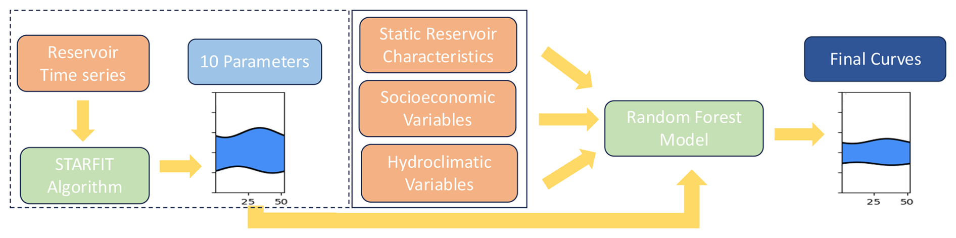
Figure 1Outlines our workflow to create the data-derived operations implemented in PCR-GLOBWB 2. Orange boxes denote the instances where outside reservoir, socioeconomic, or hydroclimatic datasets were used. Blue boxes denote the parameters and the final curves, while green boxes denote the models that we used in our methodology. For our analysis, we used 1752 reservoir time series and thus, the STARFIT maximum-minimum active zone boundaries are only available for 1752 dams. The random forest methodology allows us to extrapolate the active zone curves from these 1752 structures to 24 000 global reservoirs.
After obtaining seasonal flood and conservation pools for 1752 reservoirs, we then trained a random forest model to predict the ten parameters that determine the flood and conservation zones for these 1752 reservoirs. The random forest model used static reservoir characteristics and hydroclimatic socioeconomic variables as features. We then used the trained random forest model (Sect. 2.6) to extrapolate active storage bounds for all of the 24 000 structures and compared this new operational scheme with the current reservoir scheme in PCR-GLOBWB 2 (Sect. 2.7). Finally, we split the 22 000 dams into categories based on their main use and modelled releases based on two main operational schemes described in Sect. 2.5.2 and 2.5.3. This allowed us to analyze the bias in using different input data in our random forest workflow and the impact of operational schemes on PCR-GLOBWB 2 outputs.
2.1 Data Sets
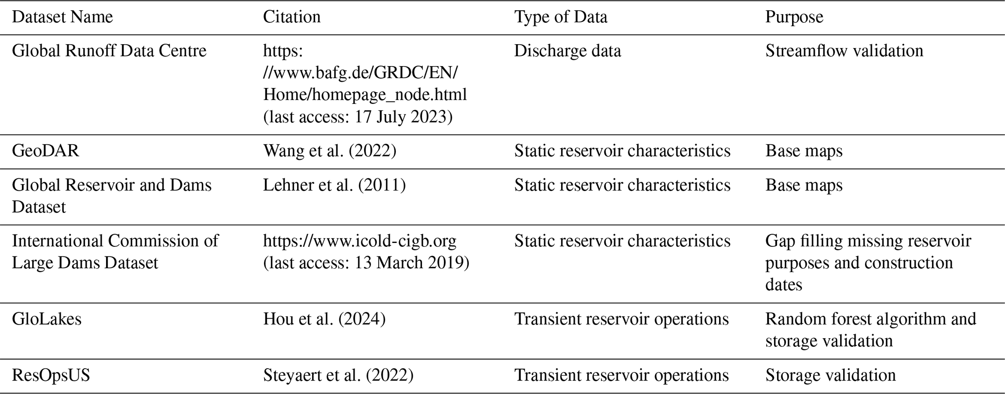
To compliment the hydrologic model and statistical model (STARFIT from Turner et al., 2021), we required a variety of datasets that are depicted in Table 1. These datasets are used to update the number of reservoirs in PCR-GLOBWB 2, train the random forest algorithm, and validate our analysis.
Wang et al. (2022)Lehner et al. (2011)Hou et al. (2024)Steyaert et al. (2022)Table 1Describes the data used in this analysis. Column one gives the dataset name. Column two gives the paper citation or webpage associated with the data source. Column three gives the type of data, and column four describes the function the data played in this analysis.
2.1.1 Reservoir Data
To update the number of reservoirs in PCR-GLOBWB 2, we used a newly minted reservoir dataset that contains over 24 000 global structures (Wang et al., 2022). The dataset itself contains static reservoir properties such as surface area, capacity, latitude, and longitude. In order to fill missing gaps in surface area, capacity, creation date, and main reservoir purpose, we linked GeoDAR (Wang et al., 2022) to the Global Reservoirs and Dams Dataset (GRanD) created by Lehner et al. (2011) and the International Commission of Large Dams (iCOLD) registry (ICOLD; https://www.icold-cigb.org, last access: 13 March 2019). From this updated table, we created annual maps of static reservoir characteristics (e.g. outlet points, storage capacity, reservoir id, and surface area), which are used as inputs to model reservoir releases and to distinguish between two operational policies hydropower-like and irrigation-like. We separated our operations into these two categories as Steyaert and Condon (2024) and Salwey et al. (2023) noted differences in operational patterns between storage reservoirs (noted as irrigation and water supply main uses) and non-storage reservoirs (such as hydropower, navigation and flood control uses).
In addition to static reservoir characteristics, we required transient reservoir data for the STARFIT model. For this, we used the GloLakes dataset (Hou et al., 2024), a dataset that contains remotely sensed reservoir surface area time series data for the majority of dams and lakes in HydroSHEDS (Giachetta and Willett, 2018). Hou et al. (2024) used remotely sensed surface area extents from Landsat and reservoir depths from BLUEDOT/Sentinel2 and other satellite products. These outputs were then put into a storage area relationship from Crétaux et al. (2016) to calculate reservoir storage. From GloLakes, we were able to fit curves for over 6000 storage structures worldwide. Due to limited satellite coverage and temporal gaps, the majority of data points sit within latitudes between 56° S and 82.8° N and are only available on the weekly time scale.
2.2 Validation Data
To validate our analysis, we used two types of validation data to benchmark the quality of the random forest model and our data-driven reservoir operations: storage data from ResOpsUS and the LandsatPlusICESat2 product from GloLakes, and streamflow data from the Global Runoff Data Center. Reservoir storage data from the ResOpsUS dataset (Steyaert et al., 2022), which contains over 600 reservoirs spread throughout the conterminous United States and was the original data (Turner et al., 2021) used to create the STARFIT algorithm, is used as an independent benchmark to evaluate how well the workflow captures seasonalities against direct observations. To validate storage changes and potential storage uncertainties within the workflow globally, we used the estimated water level variations from LandsatPlusSentinel2 and LandsatPlusICESat2, as both are available at the same temporal and spatial resolution. To validate and benchmark the addition of our data-driven operations in PCR-GLOBWB 2, we used global streamflow data from over 10 000 gages in the Global Runoff Data Center's (GRDC) dataset. The data in GRDC has good coverage over North America and Europe and lower coverage in Asia and Africa (Burek and Smilovic, 2023). Even with the limited coverage, GRDC data is still the best for global validation of streamflow. Our validation used 75 % of all the gages and of these 75 %, 8 % of the gauges have a full period of record from 1979–2023 which is the period over which we analyzed changes in streamflow due to reservoir operations. For a more detailed analysis, we removed all the gages that were not directly downstream of a reservoir and were therefore left with 2666.
All the data for this analysis was acquired through open-access sources and has been noted in either Table 1 or the Data Availability section.
2.3 PCR-GLOBWB 2
PCR-GLOBWB 2, our primary global hydrologic model, is a grid-based hydrologic model that covers the entirety of the globe (aside from Greenland and Antarctica) and estimates human water use as well as hydrological variables. The computational grid of PCR-GLOBWB 2 is available at a variety of resolutions: 30 arcmin, 5 arcmin (Sutanudjaja et al., 2018) or 30 arcsec (van Jaarsveld et al., 2025; Hoch et al., 2023). For each grid and time step (daily for hydrologic variables and dynamic for river routing), the model simulates moisture storage and water exchanges between the ground, atmosphere, and soils. Through this, it can effectively simulate transpiration from crops and vegetation, evaporation from soil and open water, snow and glacier processes such as accumulation and melt, surface runoff, groundwater recharge, soil and plant transpiration, discharge, reservoir storage, reservoir release, and runoff. The system's runoff is routed through a river network to potential sinks such as the ocean, or endorheic lakes and wetlands using the kinematic wave approach. The model currently has 6000 dams based on GRanD (Lehner et al., 2011) that use a generic operation scheme developed by Sutanudjaja et al. (2018) and described in Sect. 2.4.1. In addition to modeling hydrologic variables, Wada et al. (2014) included an updated scheme for evaluating human water use. At each daily time step in PCR-GLOBWB 2, three main steps occur: (1) water demand for irrigation, industrial, livestock, and domestic uses is estimated, (2) these estimated demands are translated into withdrawals from surface and/or groundwater sources subject to the availability of these resources and the maximum groundwater pumping capacities, and (3) consumptive water use and return flows are calculated per sector (Sutanudjaja et al., 2018).
2.3.1 Inclusion of GeoDAR into PCR-GLOBWB 2 domain
Since PCR-GLOBWB 2 runs on a gridded model domain, our first step in updating the number of structures was to create new input maps by remapping the geospatial structures from GeoDAR to the PCR-GLOBWB 2 domain. First, we rasterized the GeoDAR attributes and overlaid them on the PCRaster global domain maps that has a 5 arcmin spatial resolution (about 10 km at the equator). We opt for the 5 arcmin resolution in order to capitalize on the extensive validation and benchmarking done by Sutanudjaja et al. (2018) and to limit excessive calculation times that occur at higher resolutions (van Jaarsveld et al., 2025). We then ensured that the mapped location based on the latitudes and longitudes from GeoDAR also aligned with other reservoir characteristics such as upstream catchment area. We compared the catchment areas reported in GRanD, iCOLD, and GeoDAR to the calculated catchment area at the dam location calculated from the PCR-GLOBWB 2 drainage network. For each potential location, we minimized the difference in catchment area and the distance to the reported latitude and longitude of the dam. Due to the decision to model at a spatial resolution of 5 arcmin, we found that some dams are situated within the same grid cell. For these grid cells that had multiple dams, we summed their storage capacity and chose the construction date of the first dam. After remapping the dams to their new location on the PCR-GLOBWB 2 domain, we then ensured that reservoirs were not split between multiple catchments and that lakes and reservoirs were not mixed if situated in the same grid cell. Here, we calculated the total area of each lake and reservoir per cell, and if the total area of the lake was larger than the reservoir for overlapping structures, we converted the reservoir cells to lakes and vice versa. We ensured that reservoirs were only present in the dynamic model simulation after their initial construction date to avoid unrealistic discharge simulations. Lastly, we repeated this process with the original input data from GRanD to ensure any differences in our results could be solely attributed to the reservoir operations or initial reservoir input data.
2.4 Reservoir Operations
To evaluate the impact of “standard” generic operations and data-driven reservoir operations on global discharge, we opted to utilize two different reservoir schemes. The first is a generic reservoir scheme derived from Sutanudjaja et al. (2018) which uses static values such as maximum reservoir capacity and operational bounds: 10 % of maximum storage capacity as the dead storage (the point where water can no longer be abstracted from the dam) and 75 % of maximum storage capacity as the maximum available storage, with year-round fixed boundaries that do not reflect seasonality. The second is a data-derived reservoir scheme: STARFIT, derived by Turner et al. (2021) to fit historical reservoir time series from ResOpsUS (Steyaert et al., 2022). This method derives weekly operational bounds for flood and conservation zones from historical storage time series and has been calibrated and tested in the United States (Turner et al., 2021). As our analysis is done globally, we use data from the 1752 dams in GloLakes Hou et al. (2024) and derive the operational bounds for the STARFIT using a combination of observations and machine learning. To complement these operational bounds, we employ two main sets of equations based on two main groupings of reservoir main purposes: irrigation-like and hydropower-like (Sect. 2.5.3 and 2.5.2). We use these two groupings to denote how releases change based on reservoir storage level. In irrigation-like dams, the goal is to meet downstream demand and therefore the equations in Sect. 2.5.3 prioritize this goal by meeting all downstream demand when reservoir storage sits between the data derived operational bounds and proportionally less when storage sits between the conservation bound and 10 % of the maximum storage capacity of the reservoir. For hydropower-like dams, the goal is to hold storage as stable as possible. Therefore, the equations in Sect. 2.5.2 prioritize meeting downstream demand when the storage in the hydropower-like reservoir sits between the data derived operational bounds. However, if meeting this downstream demand causes the reservoir storage to drop below the conservation bound, then the reservoir can only meet a portion of the downstream demand to allow storage to stay in the active zone (zone between the operational bounds). For both types of reservoirs, we employ an additional flood release and account for environmental flow requirements as 10 % of the naturalized flow (Gleeson and Wada, 2013).
For all of the operational schemes (generic, irrigation-like and hydropower-like), we employ the following method. First, we define the initial release and set up the framework for other conditions, such as environmental flows and floods. To do this, we first calculate the initial discharge into the model that is defined by Eq. (1).
where RF is the reduction factor as shown in Eq. (3) with the updated values as defined above, Ravg is the long-term average outflow that is dynamically calculated within the model. This initial release (Ri) is used as a starting point in each operational scheme and is modified based on the type of operation used. In all cases, the Ri cannot be greater than the downstream bankfull discharge value of 2.3, which is the highest ratio of streamflow to stream network is expected to transport without floods occurring.
Then, we calculate the new storage using the following water balance equation under the initial release to ensure a starting point of storage:
where I is inflow, Sc is reservoir storage, P is precipitation, E is evaporation, R is release, and t refers to the time step.
We use this updated storage to define the reduction factor, which is the fraction of the long-term average reservoir release, as outlined in Eq. (3).
where Sc is the current storage level, Smax is the maximum storage capacity and Smin is the dead storage level.
After this, we employ updated release calculations based on Sect. 2.4.1, 2.5.2, or 2.5.3 depending on the type of operational scheme used as well as the type of dam. This new release is then placed back into Eq. (2) to update the storage at the current timestep.
2.4.1 Generic Reservoir Scheme in PCR-GLOBWB 2
Generic reservoir operations are already implemented in PCR-GLOBWB 2 by Sutanudjaja et al. (2018) and mimic that of hydropower operations. Each reservoir has an active zone between 10 % and 75 % of the reported maximum storage capacity in GRanD. When storage is below the dead storage limit (i.e. 10 % of maximum capacity), the reservoir does not release any water. Between 10 % and 75 % full, the reservoir outflow is scaled by the reduction factor denoted by Eq. (3).
The generic release operations are defined by the following piecewise function.
where Qavg is the longterm average discharge at the point location of the dam, Qbf is the bankfull discharge, and B is the bankfull number which is the ratio of bankfull discharge to the average discharge and is denoted as 2.3 in our analysis (van Beek et al., 2011).
In all instances, demand is set at zero, meaning that the reservoir is changing releases solely based on storage. When reservoir storage minus the projected release would be greater than the set maximum of 75 % of storage capacity or Smax, the reservoir enters flood conditions. At this point, an additional release is added to ensure that the reservoir is brought back to the upper 75 % of storage and is not over-topped. All the water is routed downstream where it can be further allocated within the river network in PCR-GLOBWB 2.
2.5 Data Driven Reservoir Operations - STARFIT
2.5.1 Operational Curves by STARFIT
To remedy gaps in generic reservoir operations (primarily the lack of demand, no environmental flow, and uniformly large active zones), Turner et al. (2021) used the ResOpsUS dataset (Steyaert et al., 2022) to create STARFIT, a reservoir model that takes historical reservoir storage, release, and inflow data to output operational ranges for each variable. To do this, these daily storage, release and inflow values are aggregated into weekly time series and a combination of sine and cosine curves (described by Eq. 5 below where μ, α, and β are curve parameters and further described in Turner et al., 2021) are fit to the upper and lower percentiles of each time series. This results in two curves bounded by the upper and lower percentiles with a total of 10 parameters, which creates a range within which reservoir release, storage, and inflow should sit based on historical data (Turner et al., 2021, used the period from 1980–2020).
For our analysis, we were only able to obtain storage time series from GloLakes, as no global dataset of reservoir releases is available. We applied the Turner algorithm to GloLakes storage data for 1752 dams from 1980–2020. This data is already aggregated weekly due to the gaps in satellite passages and therefore we were able to use the estimated storage values directly from these remotely-sensed observations. We did not gap-fill the data as this would add additional assumptions that could later lead to increased uncertainties. We fit flood and conservation curves to the 1752 dams and obtained the 10 parameters (five for the flood and five for the conservation curve) denoting the upper and lower limits of the active zone. The 10 parameters were then used as training data for a random forest model that was used to extrapolate the parameters to the global scale (Sect. 2.6).
Since there are large differences between irrigation/water supply dams and hydropower/navigation, we grouped the dams into two main categories. Main purposes, such as irrigation and water supply, were grouped as their dynamics are driven by downstream demand (either for agriculture or for domestic uses), while main purposes that have operations that are not demand-driven such as hydropower, fisheries, navigation, recreation, and other were grouped into a second category. To ensure that these two groupings had distinct dynamics, we evaluated the average, maximum, and minimum flood and conservation curves for both irrigation-like and hydropower-like reservoirs for all the 1752 training dams. These distinctions, shown in Fig. A3, demonstrate that our groupings had uniquely different conservation timeseries.This grouping allowed us to have two main operational strategies: one for hydropower-like dams which strive to keep storage as high as possible and one for irrigation-like dams which strive to meet downstream demand.
Before we could implement the data-derived reservoir operations in PCR-GLOBWB 2, we had to calculate command areas as the reservoir operation scheme requires downstream demand to determine how much water should be released by water supply and irrigation dams. Based on our literature review, we observed that there are three main command areas used by large-scale hydrologic models: 250 km (Haddeland et al., 2006), 600 km (van Beek et al., 2011), 1100 km (Hanasaki et al., 2006). For each dam represented in the GeoDAR map, we calculated the farthest location along the river network at a distance of 250, 600, or 1100 km and allocated the water demand in each cell up to this point to the upstream reservoir. If during this process, another dam intersects the river network before the full command area is created, we assume that this is the maximum distance that is served by the upstream reservoir. This command area is used to aggregate the total downstream demand that could be met by the reservoir. We use this aggregated downstream demand in both the hydropower-like and irrigation-like dams as both dam types can meet the downstream demand when storage sits between the data derived operational bounds. We found that while our model was not sensitive to the downstream area (Fig. A1), we did observe that the addition of a command area increased our model performance (Fig. A4).
Hydropower-like dams are only able to meet a portion of downstream demand when they are within their active zone and meeting demand would not decrease storage below the conservation bounds. Irrigation-like dams, on the other hand, are allowed to meet demand when in the active zone and above dead storage (denoted as 10 % of the storage capacity). We also included surface water abstractions for irrigation-like dams. In PCR-GLOBWB 2, surface water is abstracted from the river or lake cell closest to the cell with a demand. For irrigation-like dams, we only allowed surface water abstractions if the abstracted volume of water would not drop the reservoir storage below the conservation curve.
Lastly, we implement a piecewise function for releases based on the current reservoir storage (Sc) where Rf is the flood release, Env is the environmental flow requirement defined in PCR-GLOBWB 2, and Ri and Rh are the irrigation and hydropower releases in the active zone and are described in by Eq. (9) in Sect. 2.5.3 and by Eq. (8) in Sect. 2.5.2 respectively.
where .
2.5.2 Operations for Hydropower-like Dams
For the hydropower-like dams, we implement a very similar methodology to the generic reservoir operations, with the notable exception that the upper and lower operational bounds are not set at 10 % and 75 % of maximum storage capacity but rather are derived from the observational data using the workflow described in Fig. 1. We use these operational bounds to denote the active zone and therefore the release factor (Eq. 3) for the hydropower dam. We opted for different hydropower and irrigation operations as the main goal of each type of reservoir is slightly different. For example, a hydropower dam in Switzerland could have slightly different operational bounds than a hydropower dam in Vietnam, however, the main purpose: hold enough water to support electricity generation, would be the same. For all hydropower dams, we calculate a new initial hydropower release based on Eq. (7):
where D refers to the maximum demand aggregated at the specified downstream area (250, 650, 1100 km), R is the currently calculated release, RF is the reduction factor (defined in Eq. 3), Rhi is the initial release, and B is the bankfull discharge.
Once the hydropower release is calculated, there are multiple options for the final release outlined by Eq. (8). When storage is below conservation, the release is equal to the recalculated environmental flow and the dam meets no downstream demand. When the storage again enters the active zone (the area between the conservation and flood curves), the release is the difference between the current storage (Sc) and the hydropower release described by Eq. (8). If this new release results in a lower storage value than the conservation value, we assume the release is equal to the environmental flow value and does not release any additional water.
where Rhi is the initial hydropower release defined by Eq. (7), Sc is the current storage, Smax is the flood value and Smin is the conservation value.
2.5.3 Operations for Irrigation-like Dams
For irrigation-like dams, Smin is set at 10 % of the maximum storage capacity and Smax(t) is set at the flood value of that given day. When storage is in the active zone and above the dead storage zone (defined as the lower 10 %) the release will be equal to the calculated demand, unless releasing that much water would push the storage into the dead zone (defined as the lower 10 % of the storage capacity). In the case where the precalculated release is already greater than demand (Eq. 1), the release does not change. We use the following piecewise function to capture these dynamics:
2.6 Random Forest Extrapolation
Since the weekly operational bounds from STARFIT are only available for 1752 structures globally, this would severely limit our global modeling capabilities. Therefore, we used a random forest approach to extrapolate the 10 parameters for the approximately 22 000 other structures in GeoDAR based on relationships between the parameters for the 1752 dams and their reservoir and catchment characteristics. As input features, we used static reservoir characteristics (i.e. storage capacity and main purpose), socioeconomic variables (i.e. population density), and climatic variables for the upstream areas (i.e. precipitation, temperature, and aridity) to best reflect potential drivers for changes in reservoir release policies. 75 % of the 1752 structures were used to train the random forest model and the remaining 25 % were used as independent validation. Additionally, we may find that by using a different validation scheme, our operational curves may also change as our random forest is sensitive to the input data (Table A1). The obtained RF was then used to extrapolate the 10 parameters to all 24 000 structures.
Based on Steyaert and Condon (2024) and van Beek et al. (2011), we assume that the flood peak cannot be greater than 100 % or less than 5 % of the total storage capacity. Therefore, any values that sit above 100 or less than 5 for flood are automatically set at these bounds. We also assume that there is at least a 5 % difference between the flood and conservation curves so that there is always an active zone in the reservoir. To ensure this is the case, we calculate the difference between the flood and conservation curves at each weekly step for each dam and if the difference is less than 5, we use Eq. (10) below to calculate the new conservation level where is the conservation value at the current timestep, Ft and Ct are the flood and conservation values at the timestep.
2.7 Model Evaluation and Model Setup
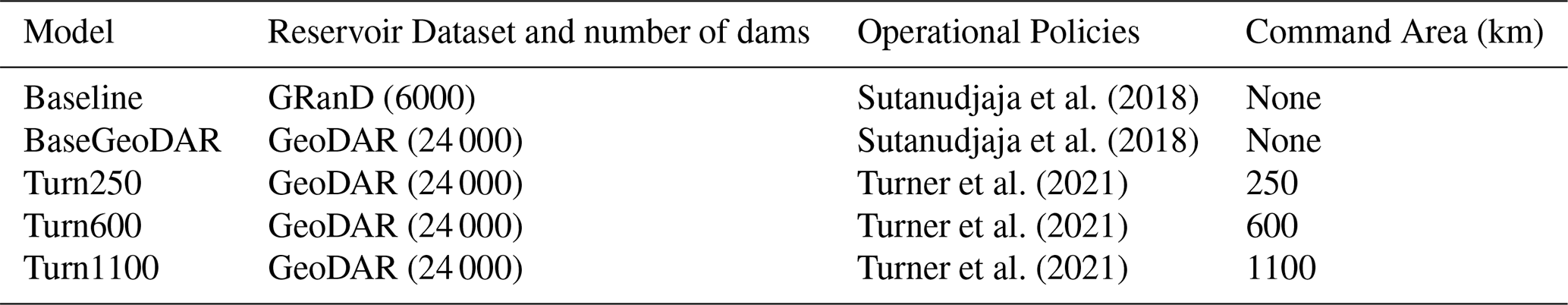
In this study, we use five scenarios to test the impact of different reservoir datasets as well as different reservoir operating schemes on the hydrologic simulations of PCR-GLOBWB 2. Our first two scenarios use the original reservoir operations in PCR-GLOBWB 2 and only differ by the reservoir input datasets (Table 2 column 2): one has the GeoDAR database as the input (BaseGeoDAR) and one has the GRanD data as input (named Baseline), both of these use the reservoir operating scheme as developed by Sutanudjaja et al. (2018). We then create three scenarios with the updated data-driven algorithm for the three command areas we opted to test based on literature: 250 km (Turn250), 600 km (Turn600), and 1100 km (Turn1100). These three scenarios use the GeoDAR reservoir dataset as the input dataset and can be directly compared to the Baseline and BaseGeoDAR scenarios that use Sutanudjaja et al. (2018).
To estimate the impact of different reservoir datasets, we compared the Baseline and the BaseGeoDAR scenarios as any difference in the hydrologic variables (e.g. discharge, reservoir outflow, reservoir storage, reservoir evaporation, surface water abstraction, and total runoff) can be related directly to the different number of reservoirs structures in the model. The comparison between the BaseGeoDAR and Turn250, Turn600, or Turn1100 serves to identify the impact of implementing a different reservoir operating scheme in an existing model like PCR-GLOBWB 2.
Sutanudjaja et al. (2018)Sutanudjaja et al. (2018)Turner et al. (2021)Turner et al. (2021)Turner et al. (2021)Table 2Shows the model scenarios that we have built and tested for this paper. The first column denotes the name assigned to the model scenario in the results.
To validate our analysis, we compared PCR-GLOBWB 2 discharge at the point location closest to dams where observed discharge is available via GRDC (Federal Institute of Hydrology, 2020). While this validation has its limitations (mainly we are only looking at single point locations and there is a skew towards more gauged basins) it allows us to observe how streamflow regimes are changing between the different simulations, how different that regime change might be between different reservoir release schemes, and to determine which reservoir operation scheme will produce the most accurate streamflow measurements. To complement this, we also validate our reservoir storage against observed storage values in ResOpsUS as well as remotely sensed reservoir storage from GloLakes to see if reservoir dynamics are better represented with the new database schemes.
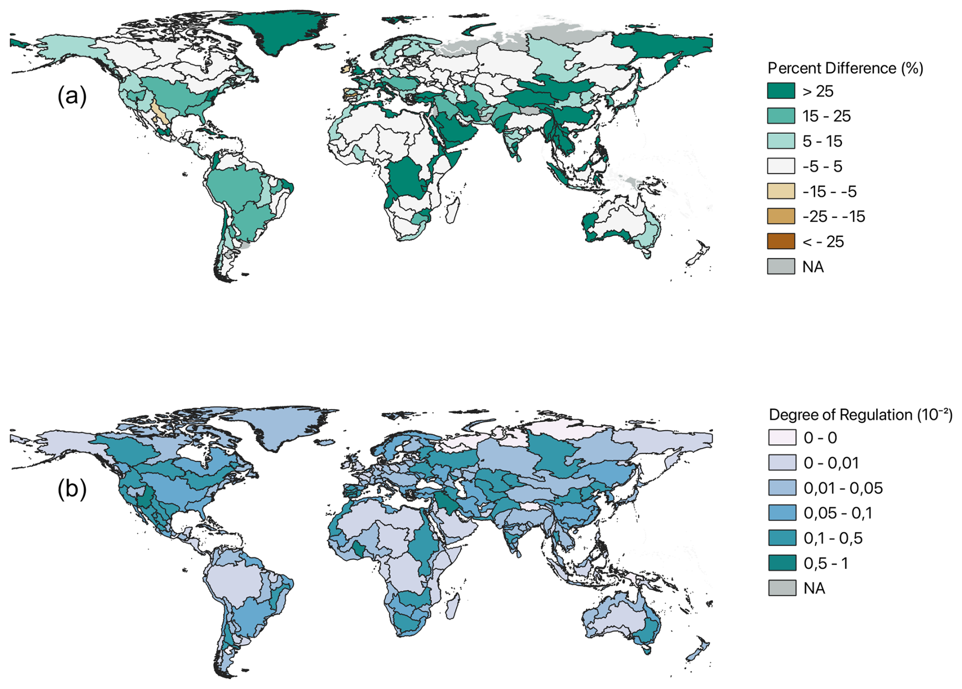
Figure 2Change in total storage globally in GeoDAR when compared with GRanD as a percentage (a) and the fraction of regulation in each basin (b) where grey represents areas that have no storage. Both panels use the PCR-GLOBWB 2 input files using GeoDAR to determine the total storage in each basin. Panel (b) uses the average of 40 years of modeled runoff data from PCR-GLOBWB 2.
3.1 Impact of reservoir datasets
We first analyze the impact of changing the reservoir dataset on the global representation of reservoirs in PCR-GLOBWB 2. Figure 2 shows the total storage that is added to the modeling domain when changing from GRanD (global storage of 6355.72 km3) to GeoDAR (global storage of 7123.66 km3). 95 % of the 230 global basins depicted in HydroSHEDS observe increases in reservoir storage as a result of the inclusion of new dams and only a few basins show a reduction. Of these 218 basins, 40 basins have slight increases in storage (noted as percent differences between 0 and 1 %), while the remaining 178 basins observe more significant increases. The largest storage increases are observed in Greenland, Central Asia, the Middle East, the Horn of Africa, and Central Africa. Of the 11 basins that do not observe increases in storage, spread throughout Central Mexico, Brazil, East Africa, China, the Baltic states, Ireland, and Spain, two observe storage percentages very close to 0, and 9 observe much larger negative differences. The lowest value sits at −21 % and is located in Ireland, which is the result of corrections in dam locations or storage volumes moving from GRandD to GeoDAR.
These negative values are the result of the two main decisions. The first is the decision to use GeoDAR as the “truth” value when reporting storage capacity, as GeoDAR included GRanD and updated these values where necessary. This decision could mean that some dams have lost storage capacity due to discrepancies between GRanD and GeoDAR. Secondly, our workflow for creating the updated input maps for GeoDAR looks at each catchment and determines the total surface area of each reservoir and lake. Since reservoirs cannot be split across multiple catchments, we calculate the total area of the reservoir in each catchment and then place the reservoir in the location that has the largest area in large with the HydroSHEDS draining network in PCR-GLOBWB 2 (Giachetta and Willett, 2018). While this is physically sound, the PCR-GLOBWB 2 drainage network might not directly align with the physical river networks, or the reservoir dataset does not align with the digital drainage network, and therefore, some reservoir structures might be oriented in a different basin. For small dams, this might not be an issue, but for larger dams, this could end up causing storage differences.
To evaluate the impact the increased number of dams has on the global streamflow, we aggregated the long-term annual average runoff from 1979–2023 across all 230 global basins and then divided the total storage capacity by the long-term average annual runoff for each basin. This yields the fraction of regulation per basin depicted in Fig. 2b. 20 % of the basins or 42 total basins have zero regulation due to having no reported storage capacity (regions depicted in grey in Fig. 2a) while 4 basins have regulation values greater than 0.5, meaning that half of the longterm basin runoff is stored in reservoirs (i.e. in the southwestern US and the Middle East).
More notable than the exact regulation values are the differences and similarities between the patterns in Fig. 2a and b. Basins with a large degree of regulation (shown in Fig. 2b), like the Colorado Basin, Yenasei, and the Tigris-Euphrates, have a large amount of storage which suggests that these regions have a multitude of medium to large dams compared to the available runoff. Conversely, some basins with a large amount of storage (Fig. 2a) such as much of Central and South Eastern Asia, Central Africa, and Western Australia do not have a high degree of regulation, which implies that there is not a direct relationship between total storage and a high degree of regulation (Fig. 2b).
3.2 Evaluation of the Random Forest Model
First, we added the 24 000 structures to the PCR-GLOBWB 2 domain and developed the workflow described in Fig. 1 to incorporate two main types of reservoir operations into PCR-GLOBWB 2. We then evaluated the impact of this methodology by using different input datasets: ResOpsUS (n=668, Steyaert et al., 2022) and GloLakes (n=24 000, Hou et al., 2024) in four different combinations. The first combination is a comparison between the different STARFIT curves obtained from each reservoir dataset (Table 3: column 1). This comparison (using 668 dams across the contiguous United States) allows us to evaluate the implicit impact of using local data (ResOpsUS) compared to a global remotely sensed dataset (GloLakes), that is required for global applications like global hydrologic model simulation. The difference we find in this comparison shows the potential reduced quality of global reservoir water level estimates compared to local information. The second combination is a comparison between the STARFIT-derived curves for ResOpsUS (Table 3: column 2) and the extrapolation of those curves (n=668) using our random forest methodology in Sect. 2.6. This allows us to evaluate how well our methodology matches the original derivation of reservoir operating curves compared to the benchmark dataset of STARFIT. The last two comparisons are between two different data products from GloLakes for satellite altimetry: ICESat2 and Sentinel2 (Table 3: columns 3 and 4), which allow us to see the difference in quality moving from local to global and using a random forest compared to the original methodology.
Table 3Depicts the performance metrics (column 1) between the extrapolated curves using the methodology in Fig. 1 and the STARFIT algorithm developed by Turner et al. (2021) to evaluate the impact of changing data and the random forest on the “original curves”. All RMSE values are in the units (% per week). Column two shows the metrics between the original curves derived from STARFIT and the constrained curves using 668 actual storage values from ResOpsUS (Steyaert et al., 2022) in order to evaluate the impact of using GloLakes. Column three depicts the RF workflow vs. the extrapolation using ResOpUS to further evaluate the RF workflow without the error in satellite altimetry. Column four depicts the comparison between the STARFIT curves and the random forest-constrained curves for the 1752 GloLakes dams that could be input into STARFIT and were used to train and validate the RF workflow. Lastly, column five shows the same metrics for another data product in GloLakes using ICESat2. This is used to validate the RF workflow.
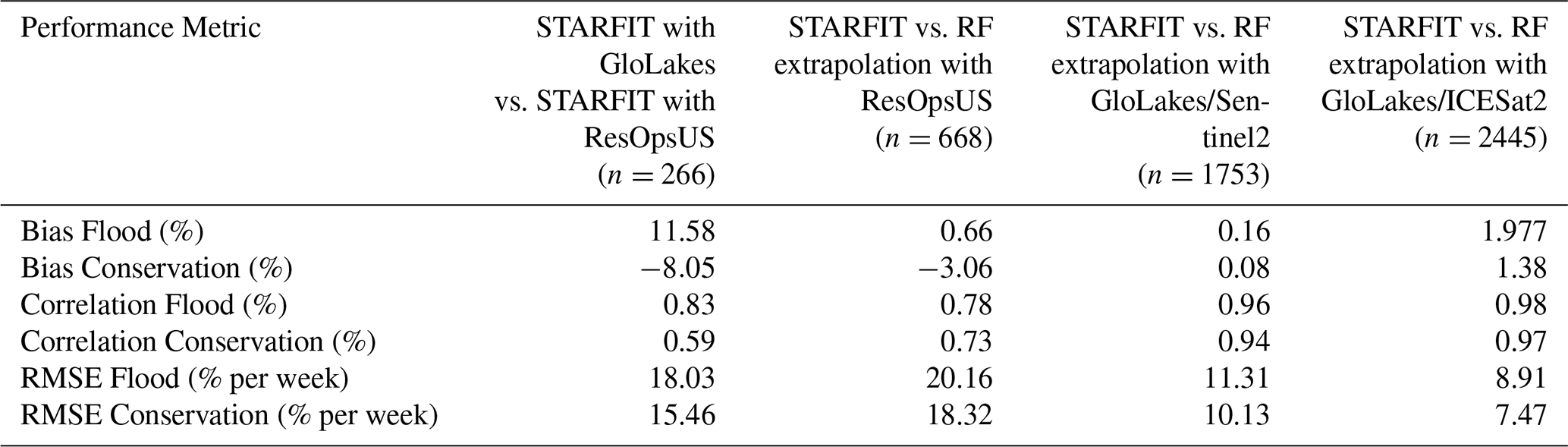
The bias metrics (given in percentages) in the first column show that STARFIT with GloLakes overestimates the flood level while the conservation level is slightly underestimated, yet the higher correlation demonstrates the timing is consistent between the two datasets. Conversely, the conservation correlation is not as strong (0.59 %), however, the conservation curves are slightly closer to the original STARFIT data than the flood curves.
After evaluating the uncertainty of the input STARFIT curves from direct observations and the satellite altimetry data (Table 3: column 1), we evaluate the extrapolation methodology in Fig. 1 with ResOpsUS (Table 3: column 2). The third column shows the bias between the random forest algorithm and the original algorithm. Overall, we observe a large bias for the flood curves and quite high correlations for flood and the conservation curves suggesting the RF workflow is overestimating the flood curves yet still aligns with the values in STARFIT. RMSE (% per week) for both the flood and conservation curves are high which demonstrates that while the timing of the flood curves match, the general errors are much larger in part because the RF algorithm underestimates the conservation levels. Compared to column two, the conservation correlations rise and the bias decreases which suggests the random forest algorithm trained on observational data does a relatively good job of capturing the levels for the conservation curves compared to the STARFIT algorithm. The RMSE values (given in % per week) do increase and the flood correlation decreases suggesting that the RF does not accurately capture the flood values potentially due to the short notice period for flood conditions.
Columns 3 and 4 show the extrapolation metrics for both GloLakes datasets: ICESat2 (column 4) and Sentinel2 (column 3). These results show that when applied to GloLakes, the RF extrapolation effectively reproduces the flood and conservation curves, even better than when the RF is applied to the ResOpsUS STARFIT curves (Column 2). However, column 1 shows that the largest error occurs when moving from ResOpsUS to GloLakes. Thus the total errors are mostly made up of errors in the storage time series that are obtained from remote sensing. In general, the operating bounds are more narrow compared to the original algorithm (Fig. 3).
While the metrics depicted in Table 3 provide a summary and validation of our workflow, the actual curves related to the different data and method combinations are much more insightful. For illustration, Fig. 3 shows the results for dams with two main purposes: the Butt Valley Dam (California, United States) with a hydropower main purpose (Fig. 3 top row) and the Medina Dam (Texas, United States) with an irrigation main purpose (Fig. 3 bottom row). We only include hydropower-like and irrigation-like as our allotted reservoir operations in Sect. 2.4 use these two categories to determine operations.
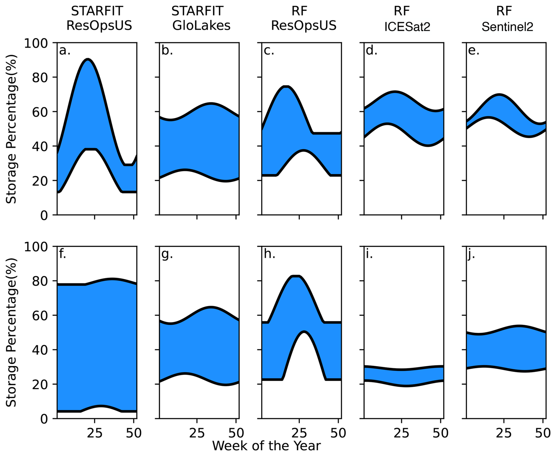
Figure 3Operational curves as storage percentage vs. epiweek for two main types of dams: hydropower (a, b, c, d, e) and irrigation (f, g, h, i, j). Panels (a) and (f) depict the original curves that come out of the STARFIT model. Panels (b) and (g) depict the STARFIT model using the data from GloLakes Sentinel2. Panels (c) and (h) depict the Random Forest algorithm trained on ResOpsUS. Panels (d) and (i) depict the Random forest methodology shown in Fig. 1 using the GloLakes ICESat2 data, while panels (e) and (j) show the final constrained curves from the random forest methodology using GloLakes Sentinel2.
When looking at the hydropower example, Butt Valley Dam, (Fig. 3: top), we observe that all the curves have a peak during the first half of the year which aligns with spring precipitation in this region. The ResOpsUS (Fig. 3a) curve has a larger peak (a range of 20 % and 95 %) when compared to the other algorithms. GloLakes-STARFIT (Fig. 3b), on the other hand, has a much more limited operational range (between 20 % and 75 %). This range is further limited when looking at the RF model using GloLakes-ICESat2 or GloLakes-Sentinel2 (Fig. 3d and e respectively), although these final storage ranges encompassed the average range of both ResOpsUS and GloLakes. The RF model with the ResOpsUS data (Fig. 3c) is more similar in range to the STARFIT curves made with GloLakes while maintaining the same peak in the early part of the year. This suggests that in general, our RF workflow constrains the active zone of the reservoir while keeping the same seasonal patterns when compared to the STARFIT curves for the hydropower-like dams.
For irrigation like dams, we plotted the same five curves for the Medina Dam (irrigation main purpose). Overall, the curves depict the same general trend (Fig. 3 bottom) with the ResOpsUS (Fig. 3f) curves having the largest active zone and the RF workflow with GloLakes-ICESat2 (Fig. 3i) having the most limited operational range. Opposite to the hydropower example, the final GloLakes-Sentinel2 extrapolation (Fig. 3j) shows a much lower overall active zone with slight increases in the active zone towards the latter part of the year, which is consistent with irrigation demand. In general, we see that moving from local data ResOpsUS to more global data like GloLakes results in the strongest reduction in the operation bounds, while moving from STARFIT to RF only results in a small reduction of the operational bounds.
To evaluate the implication of these operational bounds, we first look at the impact on two dams: the Clinton Lake Dam in Illinois (with a water supply main purpose) and the Koelnbrein Dam in Austria (with a hydropower main purpose) shown in Fig. 4. To do this, we plot the monthly average storage fraction (Fig. 4a and d), the difference between the reservoir inflow and outflow at the point location of the dam (Fig. 4b and e) and the discharge in m3 s−1 at the respective basin outlets. For each panel, we plot three of the five models: Baseline (black, the reservoir rules as currently implemented in PCR-GLOBWB 2), BaseGeoDAR (grey, original reservoir operating rules with additional reservoirs), and Turn250 (pink, new reservoir rules and additional dams). We opted not to plot all Turn600 and Turn1100 as the differences between the models are relatively small (Fig. A1). Additionally, the comparison between these dams and the rest of the modelled dams are shown in Tables A2 and A3 and additional examples of single point location comparisons are shown in Fig. A13 and additional basin outlets are given in Fig. A14.
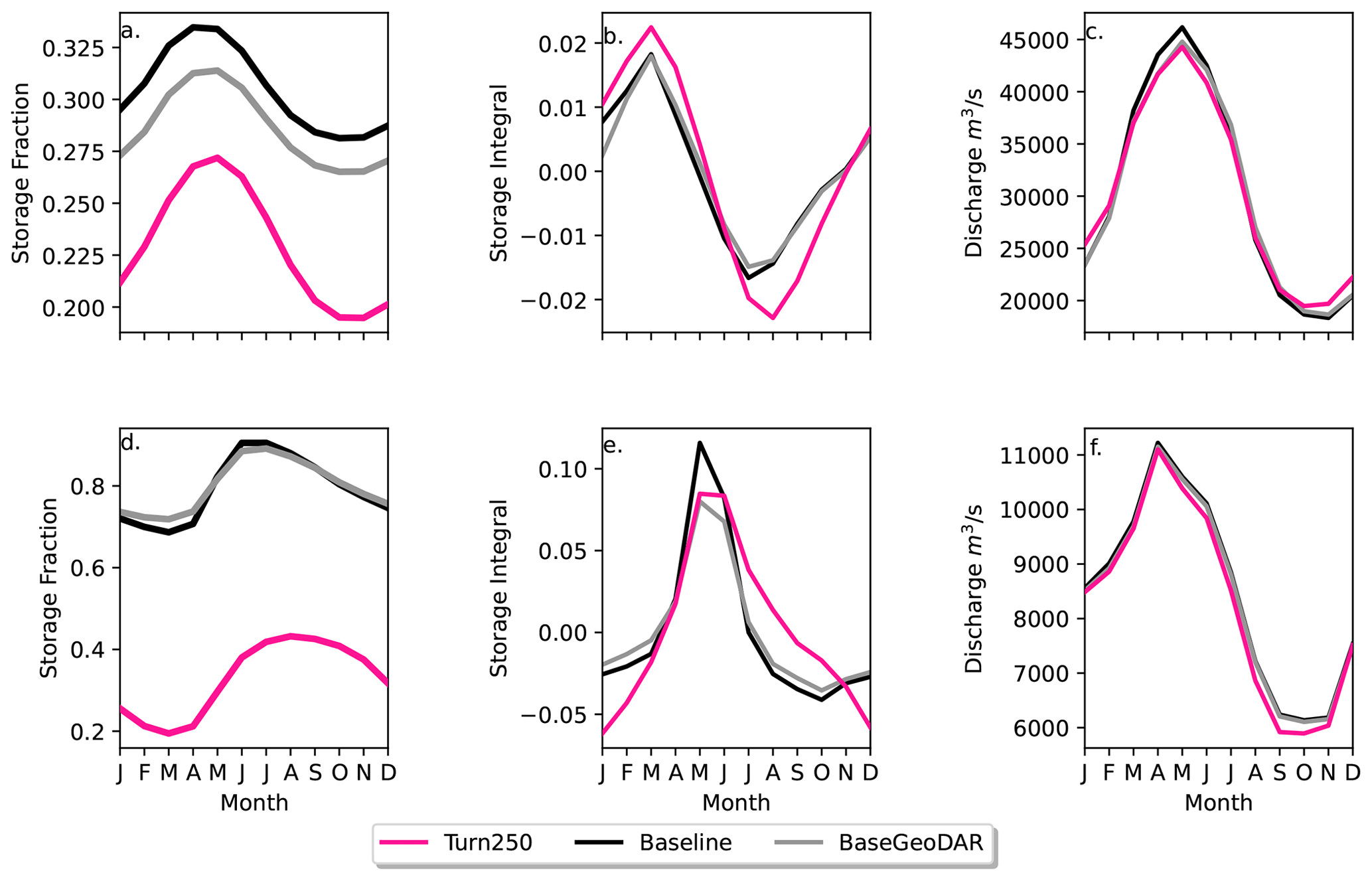
Figure 4Implementation of the final operational curves in PCR-GLOBWB 2 for the three main reservoir models: Baseline (black), BaseGeoDAR (grey), Turn250 (pink). The top row shows Clinton Lake Dam, a water supply dam in the Mississippi basin, while the lower row shows the Koelnbrein dam, a hydropower dam in the Danube basin. Column one (a, d) shows the storage fraction for all the models. The second column (b, e) shows the change in storage between each month to observe where the dams are filling (positive values and releasing (negative values). The final column (c, f) shows the long-term monthly discharge (m3 s−1) over the 40 year simulation period (1980–2023) at the respective basin outlets.
In both cases, the reservoir storage is lower in the data-driven operations (Turn250) when compared to the generic operations (Baseline and BaseGeoDAR). This is mostly due to the change in operational schemes but also affected by upstream regulation and changes therein (the difference between Baseline and BaseGeoDAR). For the hydropower dam, the Baseline and BaseGeoDAR storage fractions are not too different and have the same seasonal cycle. Conversely, the Turn250 storage fractions sit between 0.01 and 0.02 with a shifted storage fraction peak towards the end of the year compared with the Baseline and BaseGeoDAR which have a storage peak towards the spring. The water supply dam, which contains irrigation-like operations, shows similar seasonal trends as the Baseline and BaseGeoDAR, yet the average storage drops much lower, especially in the autumn and winter months.
To fully determine the shifts in storage observed in Fig. 4a and d, we can use Fig. 4b and e to determine when the reservoir is filling (positive values) and when it is emptying (negative values). In all models, the irrigation dam fills in the winter and spring and empties during the summer. The Turn250 model has slightly more filling, which is offset by more depletion in the spring months, indicating larger storage dynamics, but a lower average storage. It also does not return to full quite as quickly as the Baseline and BaseGeoDAR models, potentially due to meeting (downstream) demand. For the hydropower dam, all models have a peak in the springtime with a decrease in all other months. Conversely to the irrigation dam, the Baseline model has more filling compared to the BaseGeoDAR and the Turn250 models. That said, the springtime depletion in the Turn250 model is much more linear compared to the other models.
The different reservoir schemes have small impacts at the basin scale, even in heavily managed basins (Fig. 2). In the Mississippi (Fig. 4c), there is a small reduction in discharge for the Turn250 model during the peak flows in the spring and slightly more discharge during the low flows in the winter months. In the Danube (Fig. 4f), there is slightly less discharge at the outlet during the winter for the Turn250 model, but otherwise, the modeled discharge is the same. The difference between these two basins is in part due to the difference in regulation observed in Fig. 2b, where the Danube basin has a lower degree of regulation compared to the Mississippi basin.
Table 4Different hydrologic components for evaluating the water balance across all the models over the entire model period (1980–2022). In addition to hydroclimatic variables (precipitation, evaporation, and total water storage), we also include storage in lakes and reservoirs, evaporation from waterbodies, and abstractions from ground and surface water.
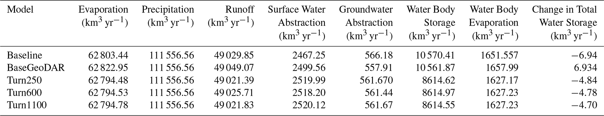
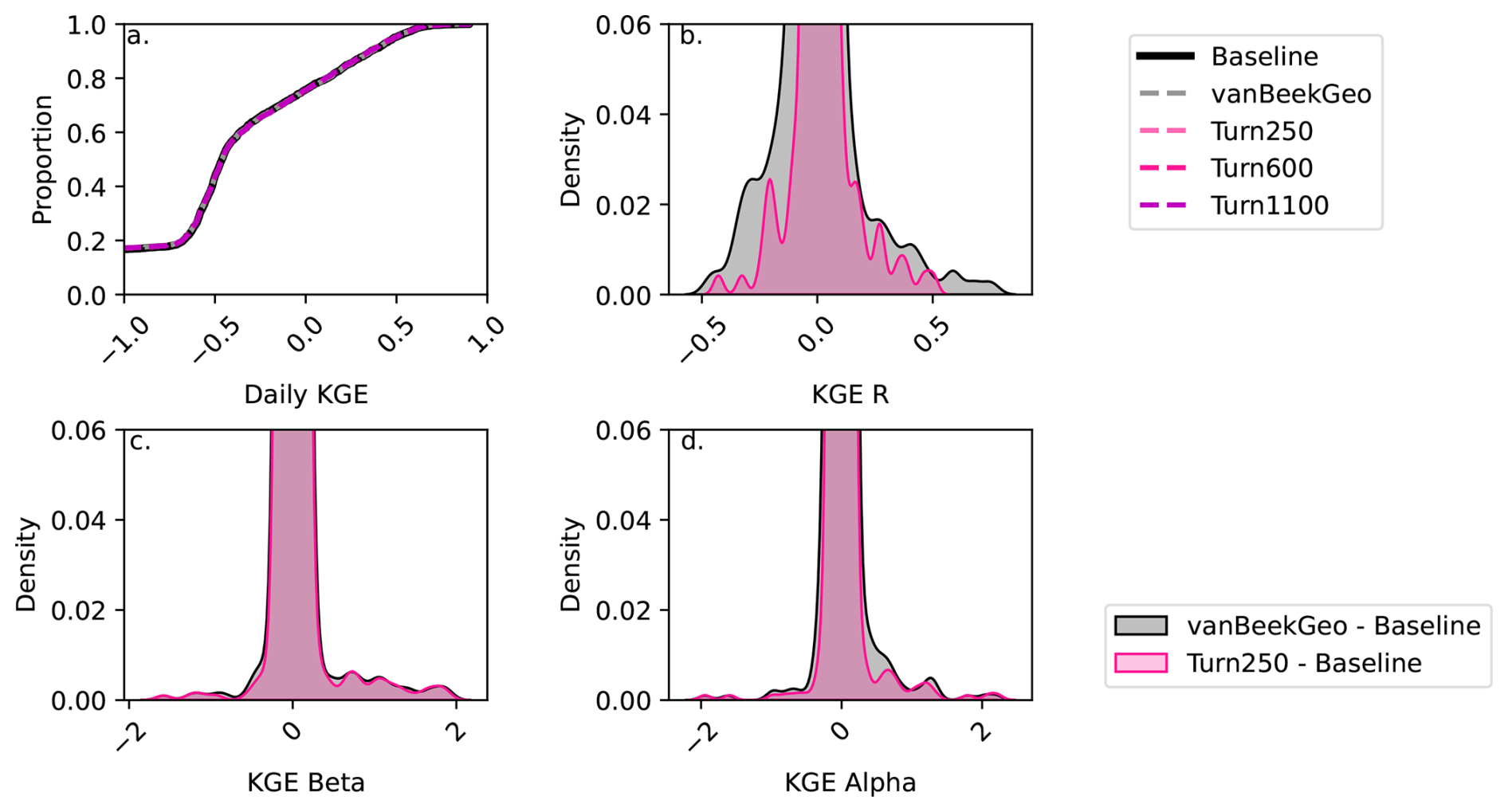
Figure 5Depicts the validation between the five models and the GRDC streamflow gauges globally. Panel (a) shows the daily KGE values for the 2666 stream gauges that have at least one dams upstream and are therefore directly impacted by our reservoir model. Each line is colored by the model. Panels (b), (c), and (d) show the difference between the baseline for the BaseGeoDAR and Turn250 models for the R (b), α (c), and β (d) components of the KGE. A plot of these values without the zoom is shown in the appendix as Fig. A15.
3.3 Reservoir model comparison and implications on storage and discharge
To validate the implementation of the new reservoir scheme, we first calculate the different water balance components (Table 4). The data-derived operations do not affect the climatic forcings; therefore, we do not observe differences in precipitation and only small differences in evaporation across all models. There is an increase in evaporation in the BaseGeoDAR model and an increase in water availability (denoted by an increase in water body storage and a positive change in total water storage across the model time frame). These increases as well as the increase in surface water abstractions are a potential result of increasing the total number of dams and the total storage capacity. Comparatively, we observe a decrease in water availability (denoted by water body storage, change in total water thickness and runoff) as well as decreases in water body evaporation and runoff in the data-derived operations (Turn250, Turn600, Turn1100) a potential result of the lower storage levels. Overall, the water balance results demonstrate that the data-derived operations do not lead to large differences across the PCR-GLOBWB 2 domain, suggesting that the relative impacts are not large and are mostly regional to local.
To further validate the data-derived operations, we analyze discharge and reservoir storage, as the water balance table shows that both are affected by changes in reservoir operations. First, we validate the discharge in our models against the observed values in GRDC. Globally, 6044 stations fit our criteria: a period of record starting in at least 1979, a minimum overlap of two or more years, catchment sizes that are at least 25 % of each other, and no more than a difference of three magnitudes between the observations and the simulated discharges. As other reservoir studies demonstrate that reservoir impacts on streamflow are greatest near the dam (Hanasaki et al., 2006; Haddeland et al., 2006; Biemans et al., 2011; Zajac et al., 2017), we filtered out any locations that were not directly impacted by upstream reservoirs. This left 2666 gauges that fit the above criteria. For these gauges, we calculated the Kling-Gupta Efficiency (KGE) and its components (correlation, bias ratio, and variance ratio) for each location and each model and plotted a cumulative distribution function (CDF, Fig. 5). The CDF shows slight improvements in the middle of the KGE range (−0.25 to 0.25), however, the improvements are quite minor. This means that our reservoir operations do not lead to significant improvements in the discharge simulations in PCR-GLOBWB 2 at the measurement locations and as a result do not allow draw conclusion into the impact of data-derived operations on streamflow regimes.
To identify the impact of the two reservoir operation schemes, we calculated the differences between the individual components of KGE (R, β, α). We included the current operational scheme in PCR-GLOBWB 2 with the inclusion of GeoDAR (BaseGeoDAR) and the data-driven operations for the 250 command area (Turn250) compared against the Baseline model (Fig. 5b, c, and d respectively). Additionally, the addition of no command area (Fig. A5a and b) demonstrated very small KGE differences. For the rest of our analysis, we decided not to include the other command areas as a boxplot of the KGEs per command area (i.e. Turn250, Turn600, and Turn1100) depicted little to no variations (Fig. A1) and the boxplot of the KGEs without the command area (Fig. A1) did not show improvements in KGE. When looking at the differences in the correlation (Fig. 5b), there are more positive correlations for BaseGeoDAR and more negative correlations for Turn250 when comparing these two models with the Baseline (42.78 % above 0 for the BaseGeoDAR operations vs. 41.46 % for Turn250 respectively). This suggests that in some cases, the inclusion of more dams is enough to improve model performance, but in most, it is not. However, the magnitude of these differences is quite small as there are only four points above or below a difference of ±0.5 for the comparison between Turn250 and the Baseline and one point for the comparison between BaseGeoDAR and Baseline. For the bias difference (Fig. 5c), the Turn250 model contains more bias values above and below 0 (50.86 % vs. 35.29 % above and below for Turn250 and 52.22 % vs. 35.15 % for the BaseGeoDAR). This suggests that the data-derived scheme is more likely to overestimate discharge than the generic operations with the GeoDAR maps. Lastly, the alpha (Fig. 5d), which depicts the variance ratio of the observations and modeled values, depicts more variance in the Turn250 model when compared to the Baseline (33.56 % vs. 40.78 % above for Turn250 and 44.78 % vs. 37.56 % for the BaseGeoDAR). This suggests that data-driven operations are better at representing the variability of discharges.
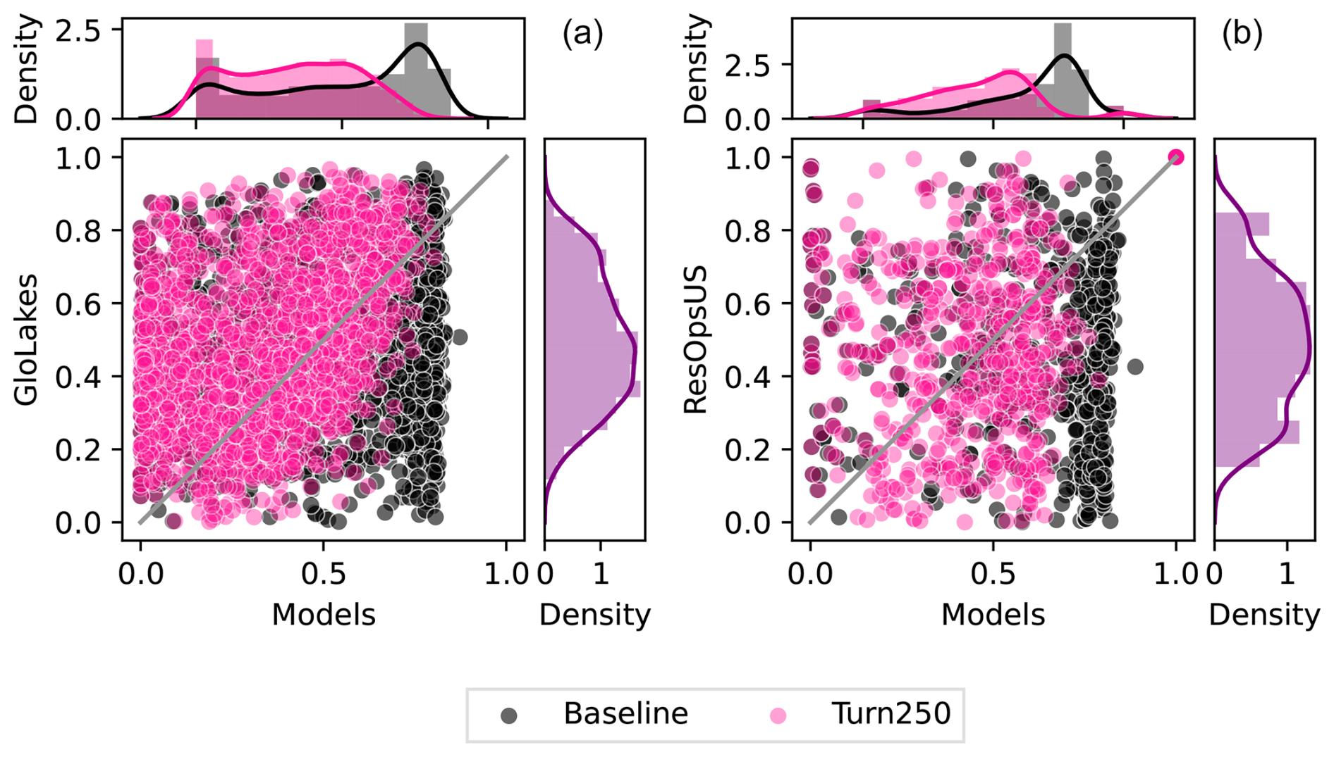
Figure 6Shows scatter plots of reservoir storage observations vs. modeled results for Turn250 (pink) and Baseline (black). Panel a uses GloLakes as the observations, which is the dataset the operational policies are derived from) while panel b uses ResOpsUS as a more “neutral” validation. For both panels, we matched the same period of record as GloLakes (1 January 1984 to 31 May 2023) and ResOpsUS (variable depending on the reservoir, but typically 1980–2020).
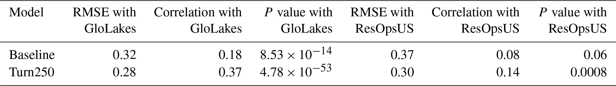
In addition, we validated the reservoir storage derived from each operational scheme against indirect observations (GloLakes) and direct observations (ResOpsUS, Fig. 6a and b respectively). To do this, we compared the long-term storage fraction for the Turn250 (depicted in pink) and Baseline (depicted in black) models against the two observations of reservoir levels. In both panels, the data-driven operations (Turn250) are more closely aligned with the observations (i.e. sit close to and above the 1:1 line) than the Baseline operations (Fig. 6). Figure 6a shows the scatter between indirect observations (reservoir levels are translated to reservoir storage) taken from satellite altimetry using GloLakes. Here, we observe that the Turn250 aligns more with GloLakes (an RMSE of 0.28 and more points at or above the 1:1 line) than the Baseline operations (an RMSE of 0.32). Next, to remove the underlying bias that we trained our RF algorithm on data in GloLakes, we also compared our data-driven operations to ResOpsUS. Figure 6b shows a scatter of the modeled storage fractions compared to observations for large dams in the United States (ResOpsUS). Once again, the Turn250 model aligns better with observations (RMSE of 0.30 for Turn250 vs. 0.37 for the Baseline). Additionally, the Spearman rank correlation between both observations and models is moderately strong for Turn250 when compared to GloLakes (0.37 for Turn250 and 0.18 for Baseline (Table 5 and slightly positive for ResOpsUS (0.14 for Turn250 vs. 0.08 for Baseline). Further analysis of the differences between the two main types of reservoirs in our analysis (irrigation-like and hydropower-like, demonstrate that our hydropower operations are more similar to the observations (RMSE of 0.28 for Turn250) compared to both the generic operations (RMSE of 0.32) and the irrigation-like dams (RMSE of 0.29 for Turn250) when comparing against the GloLakes dataset (Fig. A2). An analysis of the monthly RMSE and monthly KGE values between all the models and the GloLakes point observations also demonstrate that the Turn250 model is more aligned with observations (Figs. A7 and A8). In conclusion, this analysis demonstrates that the data-driven operations have more realistic long-term average storage compared with the Baseline scenario.
Table 5Shows the RMSE, the Spearman rank correlation and corresponding p values, between the scatter plots in Fig. 6 for each of the models (rows) and between the two datasets (columns). In both comparisons, the correlations are statistically significant.
To round off our analysis, we look at the density of all the storage fractions (Fig. 6) for GloLakes and ResOpsUS. For both of the observations, the majority of the observed storage fractions sit between 20 % and 80 % full slight variations in the exact peaks (30 % full for GloLakes and 50 % full for ResOpsUS). The storage fractions from the Turn250 operations contain more storage fraction values between 20 % and 60 % and in doing so underestimate the total storage when compared to both observations. The Baseline storage fractions, on the other hand, contain a large density of values between 60 % and 80 % full, which suggests that the Baseline operational scheme holds reservoirs at a higher storage value on average and is overestimating the amount of storage. Ultimately, we find that the storage estimates in the Turn250 model are more accurate when looking at the correlations and RMSEs.
3.4 Reservoir Regulation Changes Over Time
To determine regions where the Turn250 model is able to capture storage dynamics, we opted to look at the median long-term monthly reservoir fraction for each basin in HydroSHEDS and the aggregation per continent (Fig. 7). In addition to plotting the monthly storage fraction of all the models, we plot the monthly storage fraction for the GloLakes-LandsatPlusSentinel2 reservoirs (the training dataset for our RF workflow) to allow for comparison between observations and model results. 468 dams had a storage fraction greater than one when using the static values from our GeoDAR input maps, therefore, for these dams, we used the maximum storage value in the GloLakes observations as the maximum storage for this analysis. This misalignment could be due to flood conditions in the GloLakes reservoirs or overestimations due to the workflow in Hou et al. (2024).
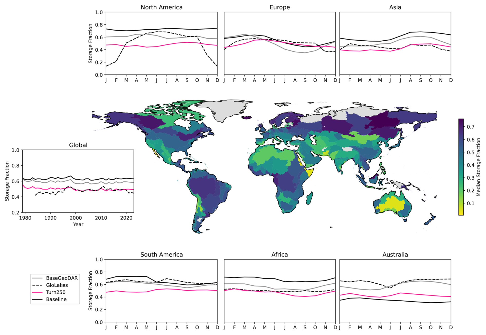
Figure 7Median storage fraction per basin in HydroSHEDS for the Turn250 as a spatial map surrounded by line plots. Each line plot corresponds to a different continent and shows the long-term monthly storage for each model: Baseline(black), BaseGeoDAR (grey), Turn250 (pink), compared with the long-term monthly storage fraction in GloLakes (navy).
In looking at the median storage fraction across the different basins (Fig. 7), we first observe higher storage fractions in the more northern basins. Basins with a large amount of regulation such as the Mississippi, Nile, and Orinoco (based on Fig. 2) have median storage fractions slightly above 0.5. The global differences in median storage fraction generally align with increased aridity, where regions that are more arid such as Australia, the Sahara, Mexico, the Middle East, and India have lower median storage fractions compared with the potential demand for water supply in these regions. Conversely, more humid regions such as Northern Europe, the Amazon, the Mekong, and the Eastern United States have median storage fractions around 0.4.
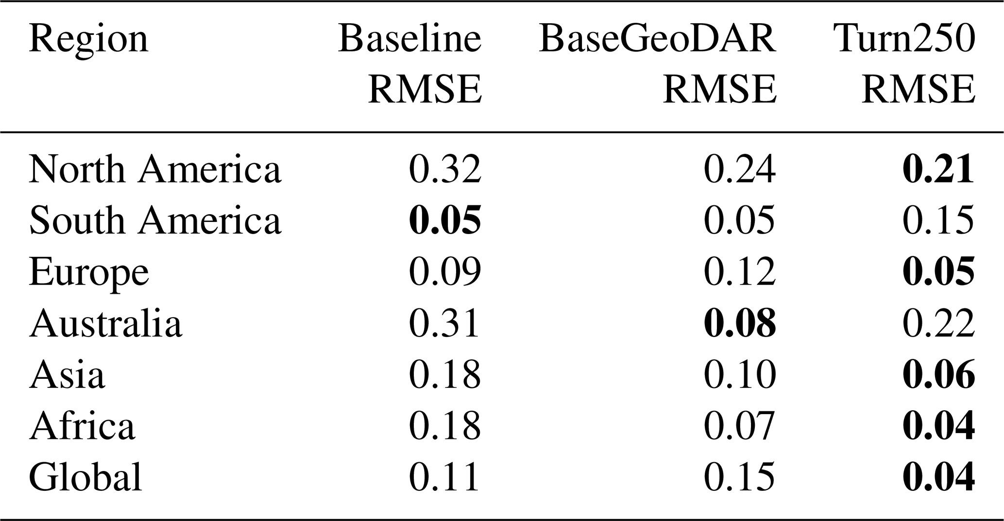
Globally, the generic operations hold more water as the Baseline and BaseGeoDAR have the higher median storage fraction of 0.63 and 0.59 respectively. Turn250 (0.50) sits closer to the median storage fraction observed in GloLakes (0.48). Regionally, though, the differences are more pronounced as the data derived operations do not capture the storage fractions observed in North America, Australia and South America, while in Europe, Asia and Africa the data derived operations align better with observations. In general, though, all the models (Turn250, BaseGeoDAR and Baseline) have similar monthly trends that do not necessarily align with the monthly trends in GloLakes. For example, in North America, the observed storage values are highest in March through July, while Turn250 has the highest storage in August to October and the Baseline and BaseGeoDAR models both have fairly flat monthly storage values. Conversely, in Asia and South America, the modeled monthly storage fraction (specifically when looking at Turn250) trend appear to align relatively accurately with the observed storage fractions.
Table 6RMSE between the curves in Fig. 7 for each of the given models (columns) and regions (rows). For this table, we took the GloLakes storage fraction as the observations. For clarity, we depict the best results in bold.
4.1 Global Impacts on the Hydrologic Cycle of the Data-Driven Reservoir Operations
To analyze the impact of the reservoir operations on the global hydrologic cycle, we first analyzed the ability of the model setup to reproduce streamflow dynamics. Primarily, we evaluate the cumulative distribution of the daily KGE values, which shows little to no difference between the different model configurations (Fig. 5a). This is partly due to the limited number of GRDC gages (only one-third) that are directly downstream of reservoirs and thus the ability of this validation to directly quantify the impact of changes in reservoir operations. While the correlations are not affected by the changes in reservoir operations, we do observe that the variance ratio shows (Fig. 5d) that the data-derived operations are slightly better at capturing the variability of the streamflow dynamics and the bias ratio shows the data-derived operations are more likely to overestimate streamflow (Fig. 5c). The sensitivity of the two operational schemes to the different components of KGE is most likely a result of the localized impacts which are more pronounced when we look at the difference between the long-term reservoir storage integral (Fig. 4b and e). While the aggregated results tend to dampen the impact of the reservoir operations on the streamflow dynamics (Figs. 4c and f, and 5a), we see that locally there are still distinct differences in the simulated reservoir outflows. In irrigation-like dams for the data driven operations, the magnitude of release is larger than that of inflow during the autumn months when compared to the generic schemes (Fig. 4c). This suggests that the addition of downstream demand into our reservoir scheme increases the overall drawdown of the reservoir and allows more water to move through the system, a dynamic observed in the scheme of Voisin et al. (2013).
Due to the limitations in monitoring reservoir impacts on global streamflow dynamics, we recommend using alternative methods such as regional or, where they exist, global reservoir storage observations. Compared to the streamflow results which do not show strong impacts, we observe that the data-derived storage is more aligned with observations and therefore provides a more accurate reservoir storage representation globally (Figs. 7 and 6). In most regions except Australia, the reservoir storage in the data-driven operations is decreased when compared to the generic operations (Fig. 7). These lower storage values are most likely due to the transference from GloLakes to the final curves using the methodology in Sect. 2.6 as this transference led to more constrained operational bounds compared to ResOpsUS (Fig. 3). We also observe that the data derived operations do not align as well as the Baseline or BaseGeoDAR for Australia and North America (Fig. 7). This could be due to data gaps in the GloLakes dataset for these regions, more hydropower reservoirs, or operational patterns that have shifted due to recent drought events, which our random forest workflow may not be able to capture as well as it does not include temporal evaluations of the operating boundaries. Additionally, we may find that by using a different validation scheme, our operational curves may also change as our random forest is sensitive to the input data. Our model water balance shows less reservoir storage, evaporation, and more surface water abstraction in the data-driven operations (Table 4). This suggests two things: first the water is moving more quickly through the river system as there is not as much storage compared to the generic operations (Baseline and BaseGeoDAR) which results in more available water for abstraction at downstream locations (shown by the difference in surface water abstractions between Turn250 and Turn1100). While this could create a water deficit in locations directly near the reservoir, the comparison with observed data in Fig. 6 demonstrates that the lower storage values are more comparable to independent observations than the larger storage values in the generic operations (Fig. 6). Therefore, this suggests that the generic operations overestimate the amount of water in storage and do not accurately pinpoint regional or localized water deficits (Salwey et al., 2023; Steyaert and Condon, 2024).
While using observed storage values is ideal for training reservoir models, the global datasets are limited by limitations in data coverage and privacy concerns (Steyaert et al., 2022; Salwey et al., 2023). Therefore, to capitalize on our global methodology, we utilized satellite altimetry data that correlates reservoir surface area with reservoir storage, instead of using observed storage values directly. Ultimately, we observed that satellite altimetry data did not reduce the overall quality of our storage results in many regions, however, the GloLakes dataset does overestimate storage in 468 of the 1752 dams in our analysis when using storage capacities from GeoDAR. While this skews the seasonal trends observed in Fig. 7, it is a result of a larger issue in data availability for reservoir management schemes. Since our analysis utilizes the general trends and dynamics in the observations to derive trends of storage fraction that are combined with reported storage capacities in GeoDAR to derive releases in PCR-GLOBWB 2, it is hypothesized that satellite altimetry is less able to capture the conservation dynamics (Hou et al., 2024; Zhang et al., 2020). However, we observe that the lack of seasonality in the conservation curves allows the random forest algorithm to better represent these curves when compared to the flood curves (RMSE of 7.47 vs. an RMSE of 8.91 for the analysis with GloLakes-ICESat2 in Table 3). The random forest algorithm trained on GloLakes has high correlations between the values from STARFIT, further suggesting that the use of satellite-derived storage dynamics is the largest area of uncertainty in our modeling framework. The biggest change is the decreased active zone both in range and in maximum and minimum values (Figs. 3 and 6). This is because satellite altimetry data uses storage-area relationships that tend to regress to the mean and that may not necessarily account for natural processes that decrease the overall amount of available storage, such as sedimentation, and are limited in their temporal and spatial resolution. Conversely, observed storage time series such as ResOpsUS use the actual storage values derived from simplified water balance equations or storage elevation relationships and contain a much larger active zone (Fig. 3). This decrease in the operational range will limit the amount of water that can be stored in reservoirs and as a result, will increase the reservoir release (Fig. 4b and e). However, we still observe through Fig. 6 that the data derived storage values are more accurate than the storage values obtained from the generic operations even with the underestimations in part because the generic operations are not as sensitive to observed changes.
4.2 Evaluation with Other Reservoir Models
Similar to other modeled reservoir operations, we observe limited improvement in discharge at basin outlets (Hanasaki et al., 2006; Haddeland et al., 2006; Biemans et al., 2011; Zajac et al., 2017), yet the data-derived storage improvements are much more similar to those of Turner et al. (2021) when using the extrapolated curves. We also observe more storage values aligning with observations for different reservoir functions. Salwey et al. (2023) noted that grouping reservoirs based on main purpose may miss key differences in the operational patterns, however, our results demonstrate that the hybrid incorporation of data-driven operational bounds with a more generic reservoir operation scheme (grouped by two main categories) performs better than the generic schemes previously used. Ideally, we would be able to differentiate into more specific reservoir categories; however, at the global scale, operational information for all main purposes (primarily for fisheries and recreation) is missing. We also find modest improvements in all major reservoir use categories (irrigation, hydropower, water supply, and navigation) by separating the values in Fig. 6 based on the main purpose (Fig. A2). Additionally, we also observe that our modeled reservoir storage aligns with the monthly trends Steyaert and Condon (2024) found in the United States (i.e. flood and navigation reservoirs sit much closer to a storage fraction of 0.3 while irrigation-dominated basins have a higher storage fraction with large seasonality). While the trends in the United States are not necessarily indicative of operational trends globally, this is one of the few studies that look directly at the trends seen in storage observations instead of solely looking at the operational impacts.
This said, our model provides a few notable improvements over other reservoir operation schemes. First and foremost, it utilizes observational data to derive key boundaries for reservoir operational bounds, something that to our knowledge, has not yet been done on the global scale (Turner et al., 2021; Yassin et al., 2019). The other reservoir schemes to utilize observational data directly typically require multiple parameters (such as in Yassin et al., 2019; Turner et al., 2021; Burek et al., 2020) or are parameterized regionally (Turner et al., 2021; Salwey et al., 2023; Brunner and Naveau, 2023; Macian-Sorribes and Pulido-Velazquez, 2020). Generic operations are typically chosen for global hydrologic models due to the ease of incorporation that relies on limited data (Haddeland et al., 2006; Hanasaki et al., 2006; van Beek et al., 2011; Sutanudjaja et al., 2018). Our scheme is scalable both to specific regions and data availability and also to model complexity. This is because the main variable of importance is the derived operational targets which can be easily obtained from limited remotely-sensed observational data.
Recently, there has been a strong push to back-calculate reservoir impacts from readily available hydrologic variables such as streamflow (Salwey et al., 2023; Brunner and Naveau, 2023). These schemes show promise in areas where reservoir data is not readily available and in models that are currently relying on generic operations based on two main purposes: irrigation or hydropower (Salwey et al., 2023). However, they still rely on the assumption that reservoir releases are the difference between naturalized streamflow and observed values (Brunner and Naveau, 2023). This can be accurate in many cases, but in human-dominated basins with a large amount of surface water abstraction and complex interactions, such as the Colorado River basin, among others, this assumption may not be valid. Salwey et al. (2023) remedied this with their transfer function approach; however, the results were only tested in water supply-dominated basins in the United Kingdom, and different balances of uses and operational patterns could change the results. Finally, in all instances, these methods assume that reservoir operations are static over time which may not necessarily be the case (Patterson and Doyle, 2019; Patterson et al., 2021) and would require nearby downstream observations of river discharge to infer the reservoir operating policies over time. While this is not infeasible, there are currently a limited number of reservoirs in the world where this would be a viable approach to accurately derive reservoir operations.
Utilizing data-driven operational bounds combined with a dual-purpose operational scheme has a plethora of benefits (more realistic operational bounds, the ability to change operations based on location, use, and hydroclimatic variables, and increased understanding of water availability). That said, there are still improvements to be made. First, the lack of global reservoir storage observations or even regional data hindered our ability to create target curves based on observations and that do not rely on satellite altimetry data and its uncertainties (temporal gaps, back-calculated storage, etc). Additionally, we assume that our operational bounds are constant during the simulation period, however in a changing climate this assumption may no longer hold, especially during extreme events (such as droughts) or under management changes (Salwey et al., 2023; Patterson and Doyle, 2019; Steyaert and Condon, 2024). We also assume reservoirs are operated as a single entity and do not explicitly and dynamically account for releases in series as we assume that the underlying storage data accounts for this dynamic and therefore these relationships exist in our operational bounds.
Apart from errors accruing from above assumptions, the accuracy of our results is also limited by the errors that are propagated through our workflow. Specifically, PCR-GLOWBWB 2 underestimates the flashiness of streamflow regimes. It is also less accurate in specific regions such as the Niger, the Rocky Mountains and portions of continental Eastern Europe due to errors in the snow dynamics, estimation of the groundwater responses and data limitations (Sutanudjaja et al., 2018). Additionally, the estimation of the operational STARFIT rules from the remotely sensed storage data of GloLakes is limited by the revisit time of satellites, the influence of cloud cover and atmospheric interference as well as the statistical models that back calculate storage that are limited by the digital elevation model's spatial resolution (Hou et al., 2024; Chen et al., 2022). As storage is typically not a direct measurement and, even in the case of in-situ observed water levels observations, is back calculated from storage/area or storage/elevation relationships, validation primarily on storage alone is inherent to uncertainty. Primarily, these limitations can affect the actual storage value as they rely on storage elevation charts that are only periodically updated (Steyaert et al., 2022). While the single errors are propagated through our system, the results of the independent validation with ResOpsUS and GloLakes (Figs. 6 and 7) show improved performance for storage values in PCR-GLOBWB 2 and suggest similar improvements for other global hydrologic models with the caveat that errors may propagate through the modelling system.
Based on these limitations, we find that more effort needs to be put into cultivating global datasets of historical reservoir operations and also include more data-derived methods in operational reservoir schemes. While the first recommendation is liable to privacy concerns (Steyaert et al., 2022), we believe that more accurate information on reservoir operations will increase the reliability of large-scale hydrological models and thus serve a wider community. The addition of more data-derived methods in our reservoir operations scheme demonstrated much lower storage than PCR-GLOBWB 2 had previously modeled using other methods. This could highlight unknown water deficits as the total reservoir storage in select regions may not be able to account for surface water abstractions and the currently implemented reservoir operating rules could overestimate the amount of available water in vulnerable regions.
This study combines previous work by Turner et al. (2021) and data acquisition by Hou et al. (2024) to develop a workflow for implementing data-driven reservoir operations in global hydrologic models. Using an updated dataset of reservoir locations (Wang et al., 2022), satellite altimetry data from Hou et al. (2024) and the STARFIT model (Turner et al., 2021), we first developed operational bounds for 1752 reservoirs whose storage time series were estimated using remote sensing that are then used to train a random forest algorithm. We observe that the RF extrapolation is accurately able to depict the flood and conservation curves and that the main source of uncertainty is the errors associated with the storage estimations from satellite altimetry. After this evaluation, we then estimated operational bounds for over 20 000 structures that are implemented into PCR-GLOBWB 2 using the trained random forest algorithm. While the impact on discharge is modest and does vary significantly based on location, we see large improvements in our reservoir storage and seasonal dynamics when using data-derived operations over the generic ones. Therefore, we suggest reservoir operation models rely emphasize model validation on reservoir storage in addition to validation based on streamflow in place of validation solely on streamflow as the available streamflow observations are rarely close to the release point of the reservoir and therefore not as sensitive to reservoir operations compared to storage. We also do not see strong differences when using different command areas even though it would be expected that changes to these values would increase or decrease storage. We did however observe slight improvements when using command areas compared to without command areas. This suggests that reservoir modelers should use a command area, but can opt to use the command area that makes the most sense to their domain (we opt to use the 250). To remedy issues with the static operations (i.e. no change in the future), in the future we hope to evaluate changes in operational patterns using smaller 10-year moving periods to see if there are large changes in operational dynamics. We hope that this work can be further implemented into other large-scale hydrologic models to better represent reservoir dynamics and to evaluate their impact on hydrologic regimes and anthropogenic water availability.
In the below figure (Fig. A3), we plot the average, maximum and minimum value of the derived STARFIT curves for the irrigation-like (blue) and hydropower-like (red) dams for both the flood (Fig. A3, top row) and the conservation (Fig. A3, bottom row) bounds. While the average and maximum flood and the maximum conservation values do not differ much between the dams, we do see large differences in the average conservation and the minimum flood and conservation curves which could be a result of the differing operations at the lower end of storage. Specifically, the flood minimum peaks in irrigation-type dams in the spring and summer months to potentially support downstream demands in drier periods, while the hydropower-like dams have lower flood minimum values. The conservation curves experience the most changes in part due to the hydropower-like dams holding storage much higher across the year while the irrigation-like dams are meeting downstream demand in the autumn months. For the minimum conservation values, the irrigation-like dams have higher storage fractions compared to the hydropower-like dams. Due to the differences in the seasonality of the lower bounds for the flood curve and the differences in the conservation curves, we still think that the distinction in operational schemes is useful.
We computed the daily KGE values for these two models as well as the Turn250, Baseline and vanBeekGeo against the streamflow observations in GRDC. While the addition of the command area slightly improves the model (Fig. A4, purple vs. pink lines), we do see large improvements in using two different operational schemes (green vs. pink lines in Fig. A4). This suggests that creating two different release rules for irrigation-like and hydropower-like dams enhances model performance compared to a single simplified scheme. We also saw there are operational differences in the average conservation curves and the flood and conservation minimum curves when looking at the two typologies we defined (Fig. A3). This, in conjunction with Steyaert and Condon (2024) and Salwey et al. (2023) noting that there are differences in irrigation, water supply and hydropower dams, further supports our conclusion that having two main types of reservoir operations better represents the observed dynamics.
We computed the daily KGE values for different command areas: 250, 600 and 1100 as well as for the Turner scheme without command areas. While the lack of command area leads to worse KGE values for all station locations, the lack of command area does lead to limited improvements in some areas. Aggregating these performances into the boxplot in Fig. A1 shows that while the variance in KGE values are lower, the average performance is actually slightly below that of the other command areas. Therefore, we opted to continue our analysis with the Turn250 model.
We decided to implement a simple rule curve for the Mississippi Basin that accounts for the downstream demand (the green line in Figs. A4 and A6). This simplified operational policy still accounts for downstream demand according to the 250km distance and can meet this demand and surface water abstractions if storage is within the active zone (defined as the area between the flood and conservation curves) and includes environmental flow and flood releases. We ran the model for the Mississippi basin without the command area (by setting the downstream demand to 0) but including the two operational schemes (purple line). In analyzing the longterm monthly storage for the simple rule curve we observe that we hold less water on average, but the seasonal dynamics are similar to the other models (Fig. A6). This suggests that the biggest difference is the overall storage fraction levels and this simplified rule curve decreases the overall water availability in the Mississippi region.
The below figures shows the evaluation between the three main operational scheme models and the point observations in GloLakes. The KGE plot shows that the Turn250 model has relatively more negative KGE values, however, these negative performances are typically in wetter periods where PCR-GLOBWB 2 is already underestimating streamflow. This model also has larger KGE values. As for the RMSE we do see that the Turn250 has more values closer to 0, suggesting the Turn250 model is more aligned with the observations. We also opted to plot the KGE components (Fig. A8).
The alpha and R components show slight improvements in modeled storage with the Turn250 operations, while the beta shows that the Turn250 has more bias, which is most likely occurring in the wetter periods.
To evaluate the difference between the GloLakes curves in Fig. 7, we evaluated the number of dams in the GloLakes vs. GeoDAR (Figs. A10 and A11) as well as the RMSE and KGE for the US dams (Fig. A9.The number of dams in the US in GloLakes (1752 with 543 or 31 % in the US plotted in red in Fig. A10) differs from the total number of dams used in our analysis (over 20 000 with 8214 or 40 % in the US plotted in blue in Fig. A11). Additionally, the random forest algorithm looks for similarities and differences across all the dams in the training set. This training set (75 % of all the data) is chosen randomly and, while it includes dams from the US, we make sure to choose multiple regions. Therefore, this could account for the regional differences in our storage patterns compared to the GloLakes observations. When plotting the monthly KGE and monthly RMSE (Fig. A9) for each of the models, we do see that the RMSE in the United States are much higher and the KGE is slightly worse. This suggests that the issue in performance is perhaps due to the underlying model dynamics in PCR-GLOBWB 2 as well as the inclusion of other regions in the training dataset to create the Random Forest algorithm.
To show the difference between the different components of the KGE in Fig. 5, we created scatters plots of the different KGE components between the Turn250 and vanBeekGeo models (Fig. A12). While the scatter for the R component makes this component appear to be the most important, we find that both the R and beta components have almost equal values above and below the 1:1 line, suggesting that these two components are muting the KGE differences. Comparatively, alpha has 1196 points above the 1:1 line and 779 points below the 1:1 line which suggests that alpha is the most sensitive to the operational changes and contributes the most to the KGE changes (1210 above the 1:1 line and 1158 below the 1:1 line).
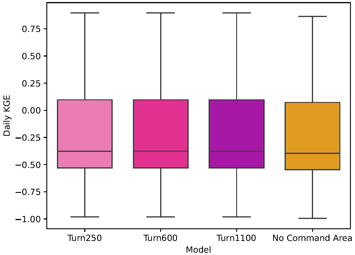
Figure A1Shows a boxplot of the data derived operational scheme with the three main command areas: 250, 600 and 1100, in different colors. The Turner scheme with no command area is shown in orange.
Table A1RMSE between the curves in Fig. 7 for each of the given models (columns) and regions (rows). For this table, we took the GloLakes storage fraction as the observations. For clarity, we depict the best results in bold.
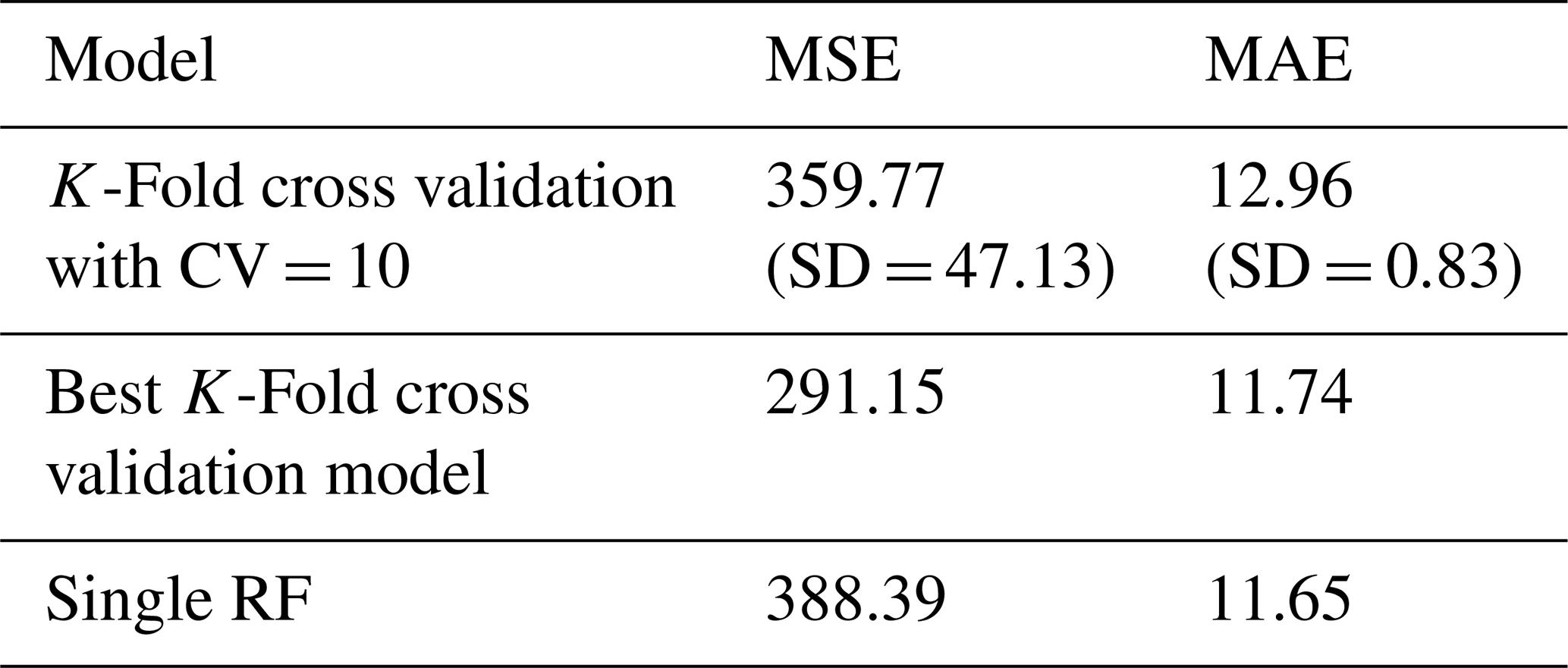
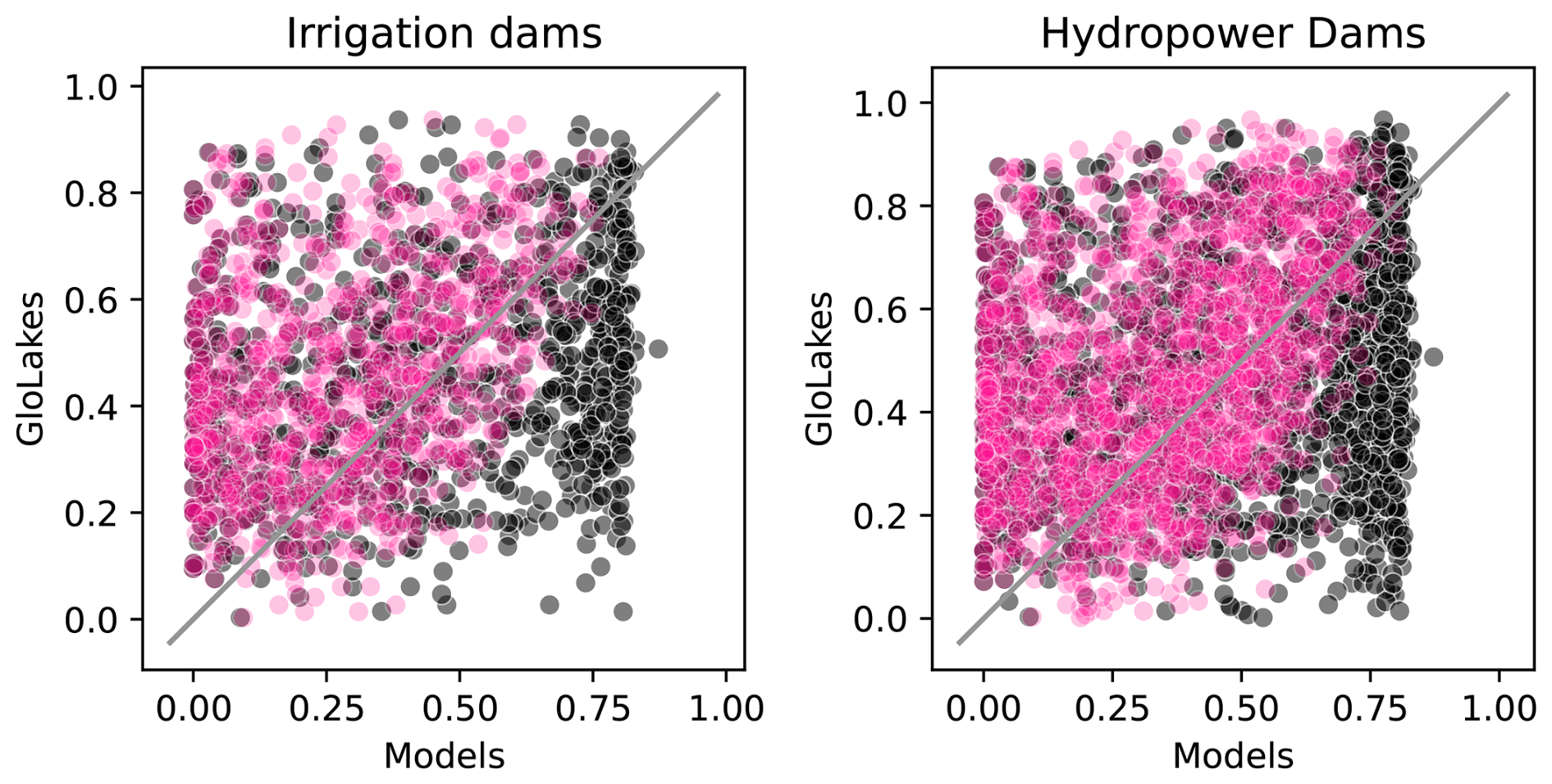
Figure A2Depicts a scatter plot of the storage fractions in GloLakes vs. the storage fractions in Turn250 and Baseline models. The left panel shows the results for dams with an irrigation main purpose and the right panel shows the dams with a hydropower main use.
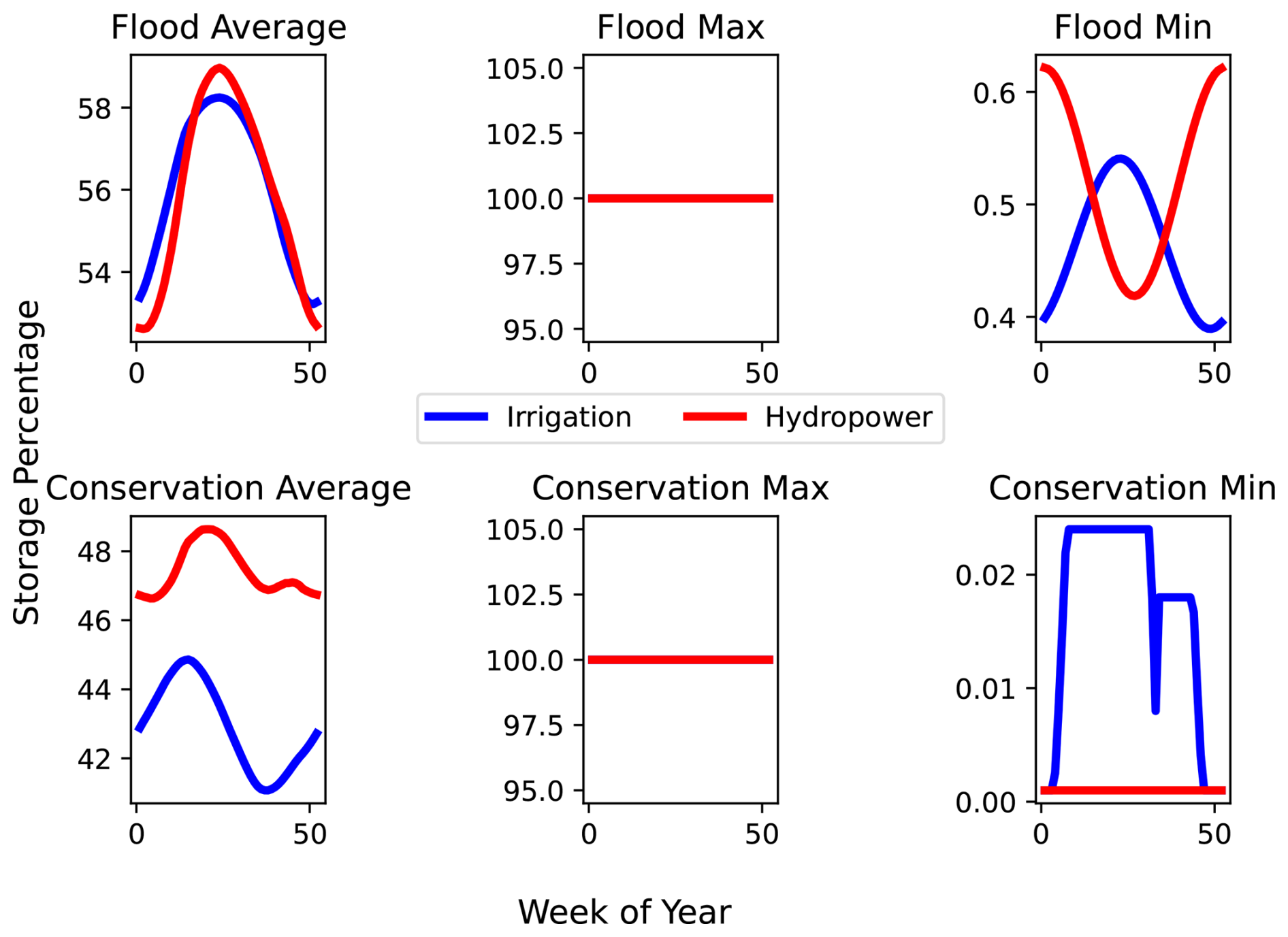
Figure A3Shows the average, maximum and minimum conservation and flood timeseries for all 1752 STARFIT curves that are employed in the random forest algorithm colored by main use denoted in our analysis. The blue curves are indicative of the irrigation curves and the red are the hydropower curves.
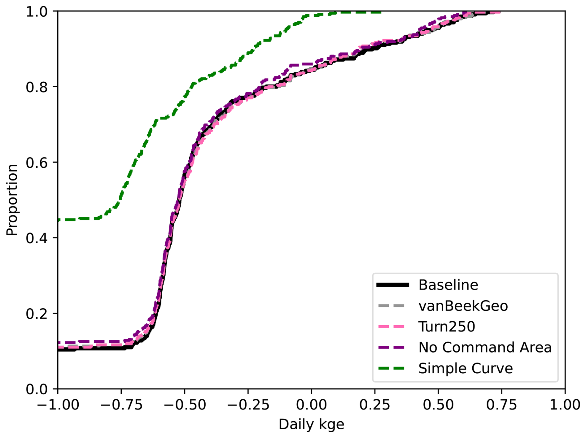
Figure A4Depicts the cumulative distribution function of the three main models in our analysis: Baseline (black), vanBeekGeo (grey), Turn250 (pink), as well as two additional tests with removing the command areas (No Command Area in purple) and a simplified release method (Simple Curve in green). As the Simple Curve and the No Command Area curves were only evaluated for the Mississippi basin, we only included the daily KGE values in the Mississippi basin for other models.
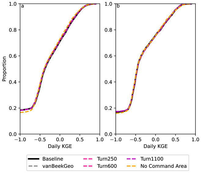
Figure A5Depicts the cumulative distribution function of the daily KGE values of the three main models in our analysis: Baseline (black), vanBeekGeo (grey), Turn250 (pink), and the run with no command areas (orange). Panel a shows the cumulative distribution of the daily KGE for all the GRDC gages, while panel b shows the daily KGE for the 6000 gages that are downstream of dams.
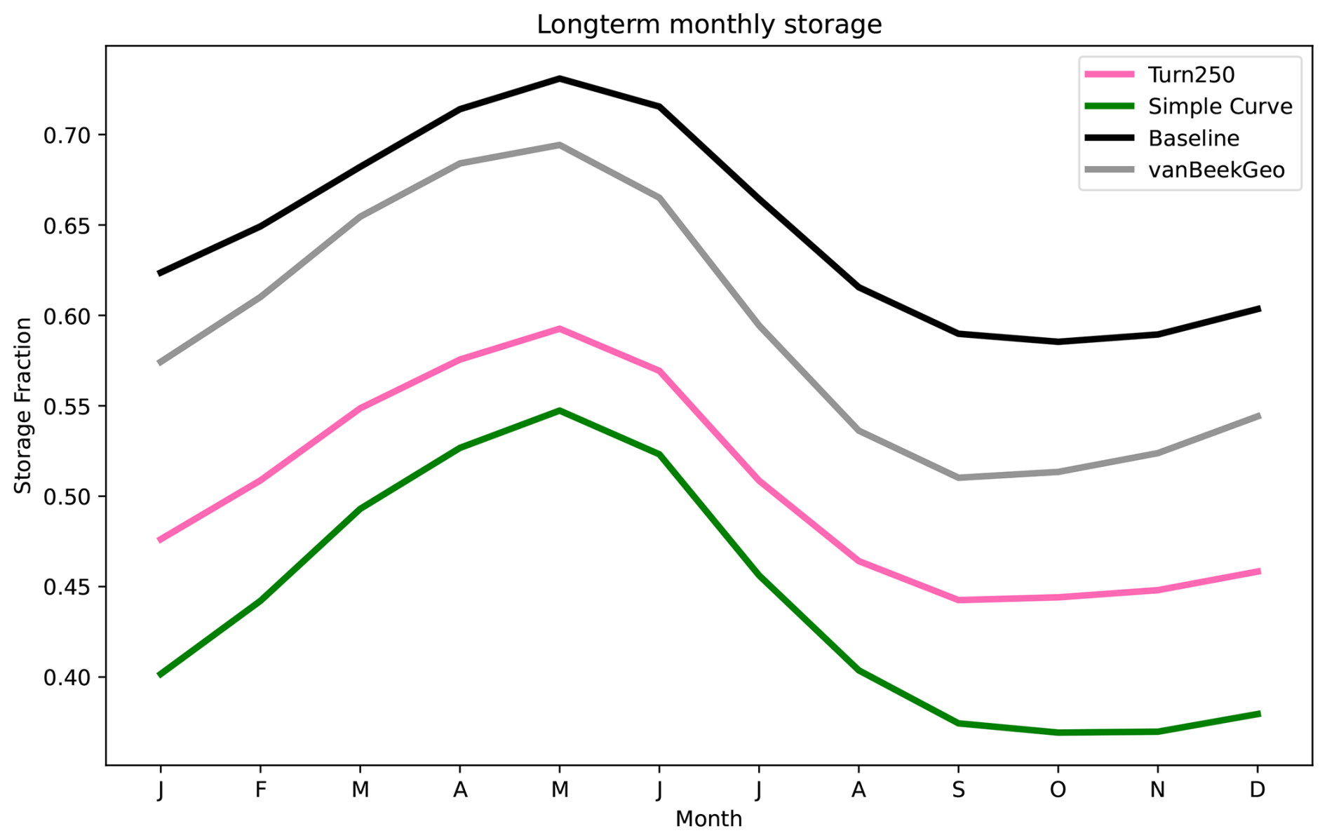
Figure A6Depicts the longterm monthly average of the storage fractions for the three model in our analysis: Baseline (black), vanBeekGeo (grey) and Turn250 (pink) as well as the simplified release curve denoted as Simple Curve (green).
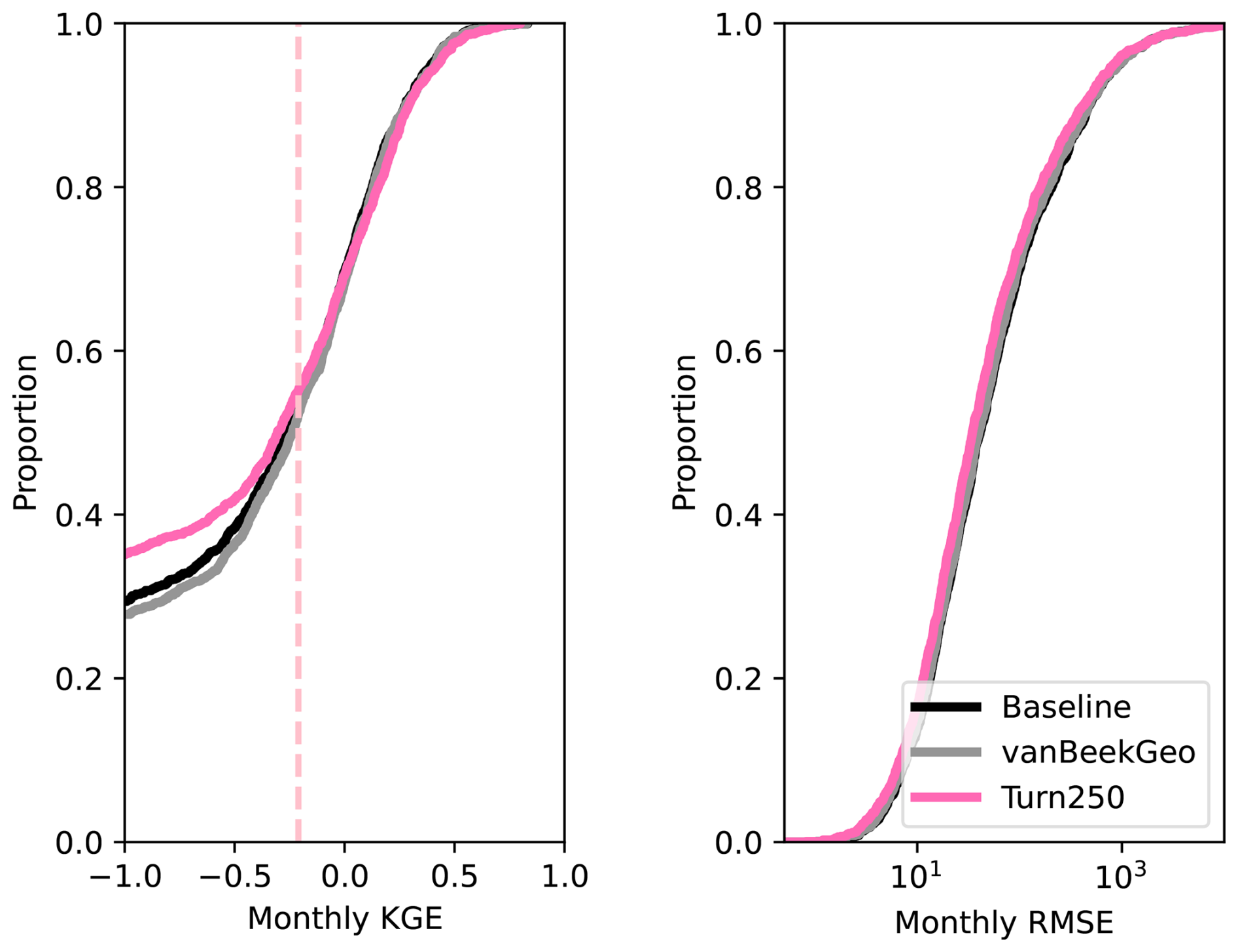
Figure A7Cumulative distribution functions of the monthly KGE and monthly RMSE between the three main models: Baseline (black), vanBeekGeo (grey) and Turn250 (pink) evaluated against point observations in GloLakes.

Figure A8Shows the cumulative distribution functions of the KGE components, α, β and R between the three models: Baseline (black), vanBeekGeo (grey) and Turn250 (pink) evaluated against point observations in GloLakes.
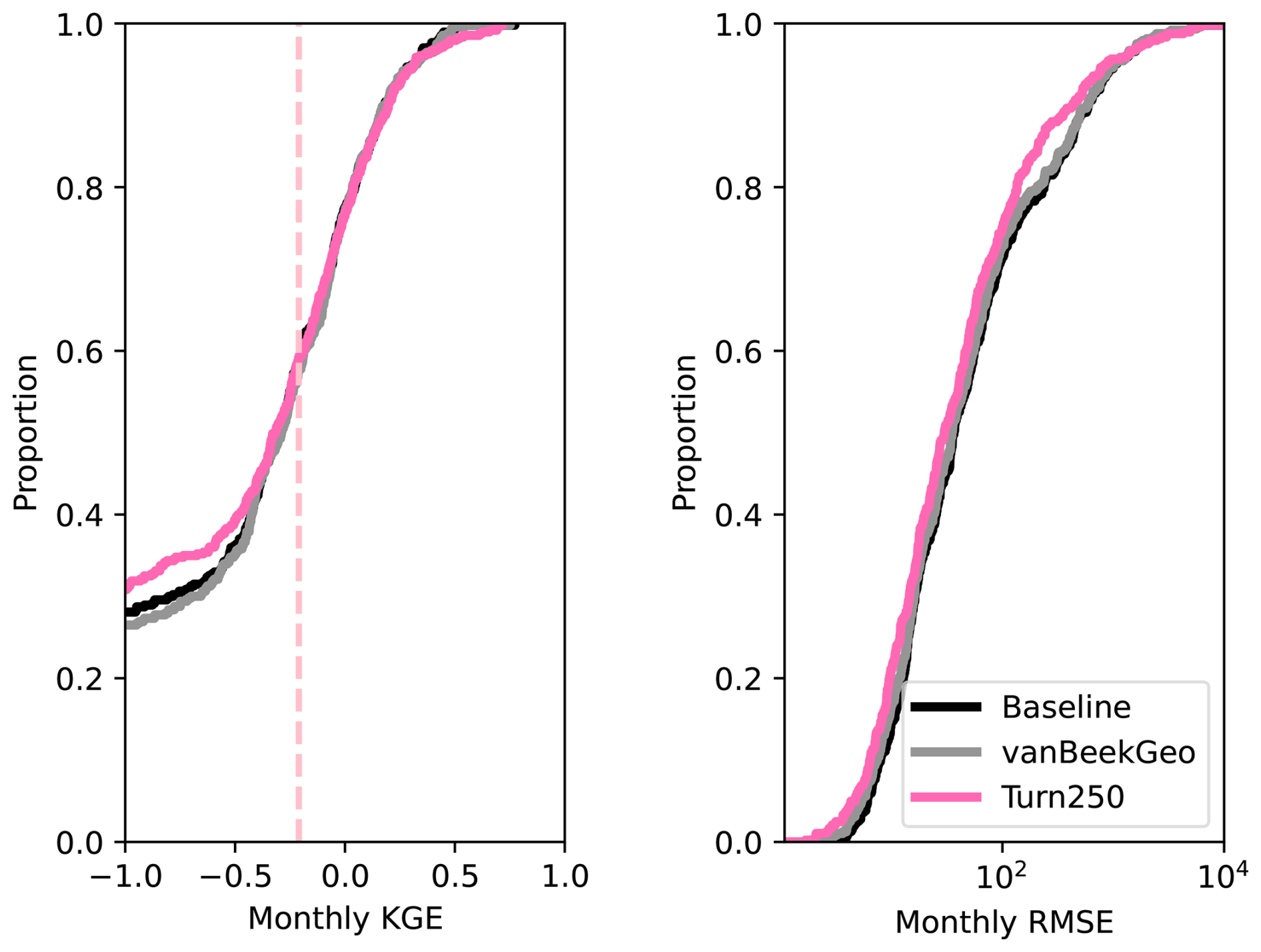
Figure A9Depicts the KGE and RMSE CDFs for the storage evaluation with point location in GloLakes across the United States. The simulated models are depicted in black for Baseline, grey for the vanBeekGeo and pink for Turn250. The dashed pink line denotes the boundary above which the KGE values show significance.

Figure A10Map of the point locations of the GloLakes observations used to train our random forest algorithm and validate our analysis.
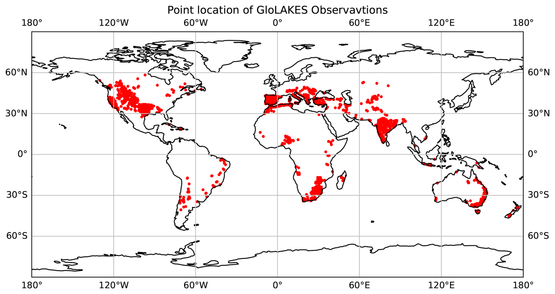
Figure A11Point location map of all GeoDAR locations that are used in our analysis.
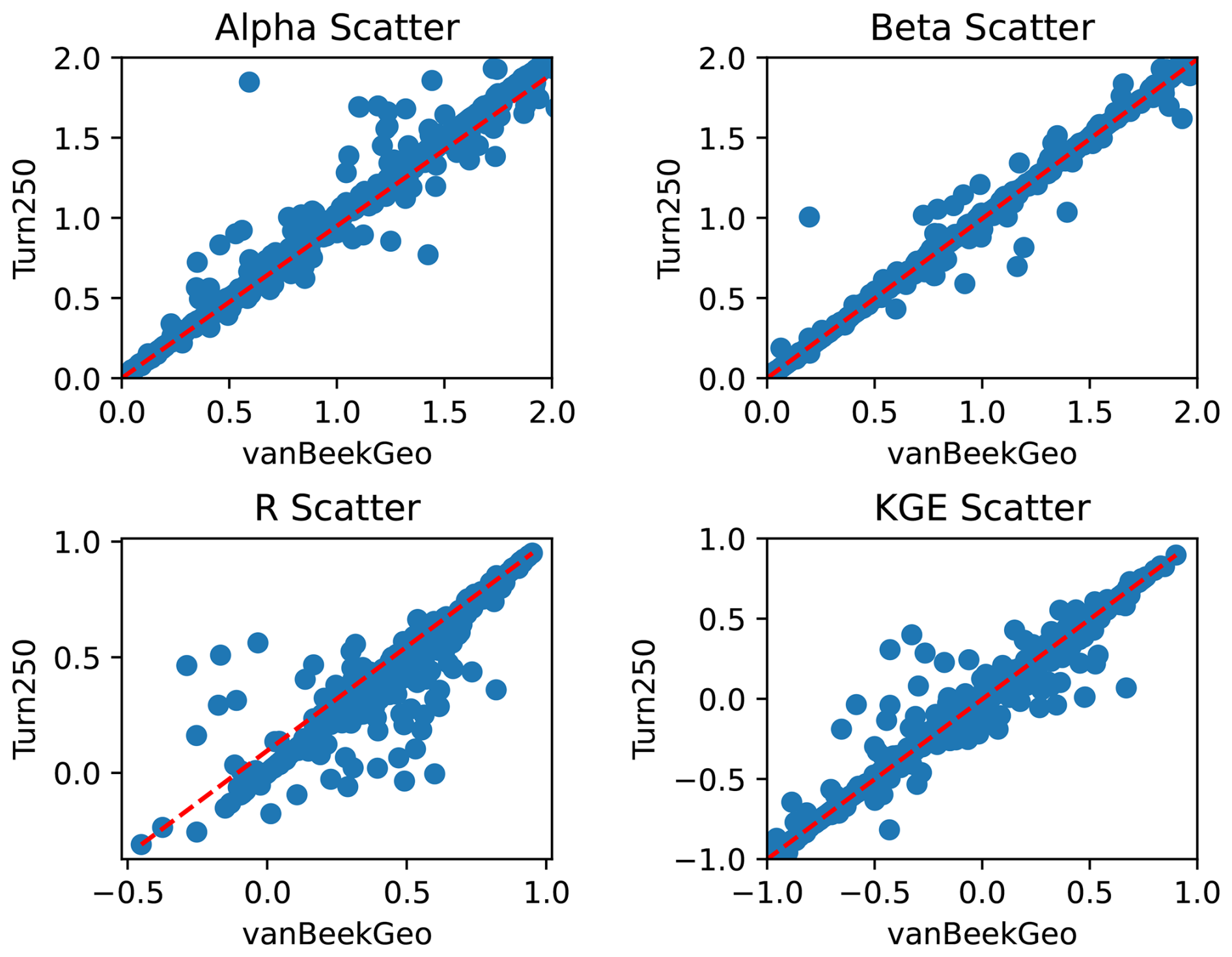
Figure A12Scatter plots of the streamflow KGE components between each model and observations. We plot the KGE components (α, β, and R) for the Turn250 model on the y axis and the KGE components for the vanBeekGeo model on the x axis. The dashed red line is the one-to-one line.
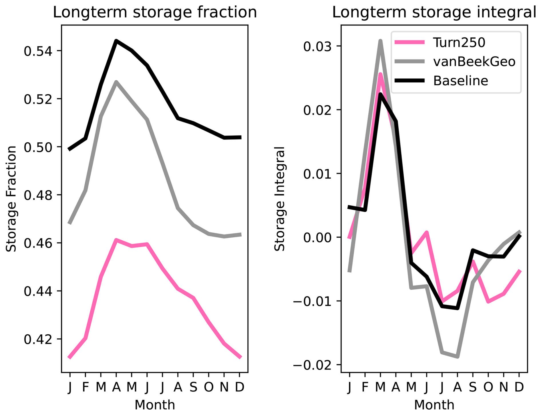
Figure A13Plots of the longterm storage fraction and the longterm storage integral for the three models: Baseline (black), vanBeekGeo (grey) and Turn250 (pink).
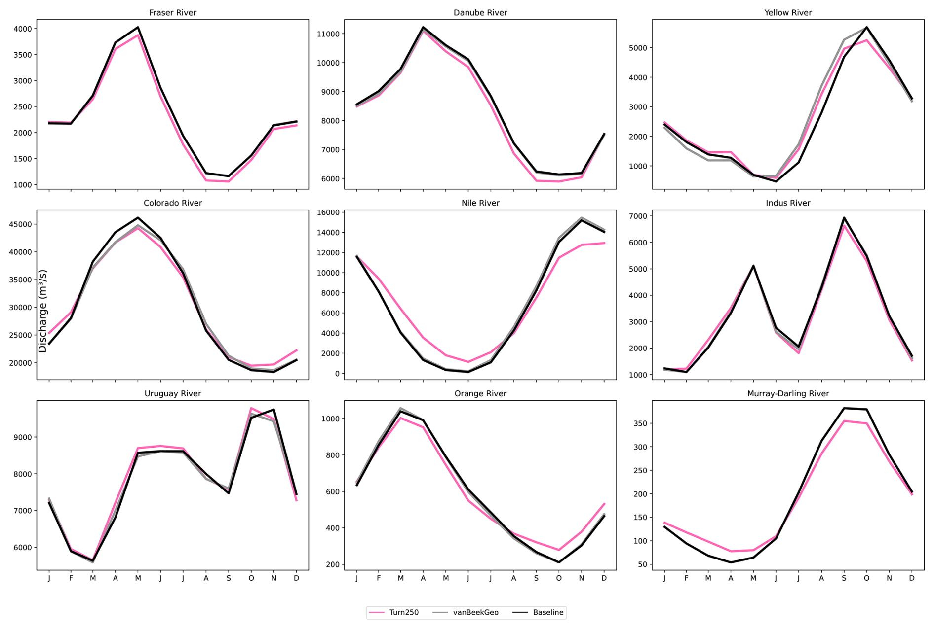
Figure A14Depicts the longterm monthly averages of an additional nine global basins ordered by location. All plots include the same three main models: Turn250 (pink), vanBeekGeo (grey) and Baseline (black), to see the changes in discharge for additional basins.
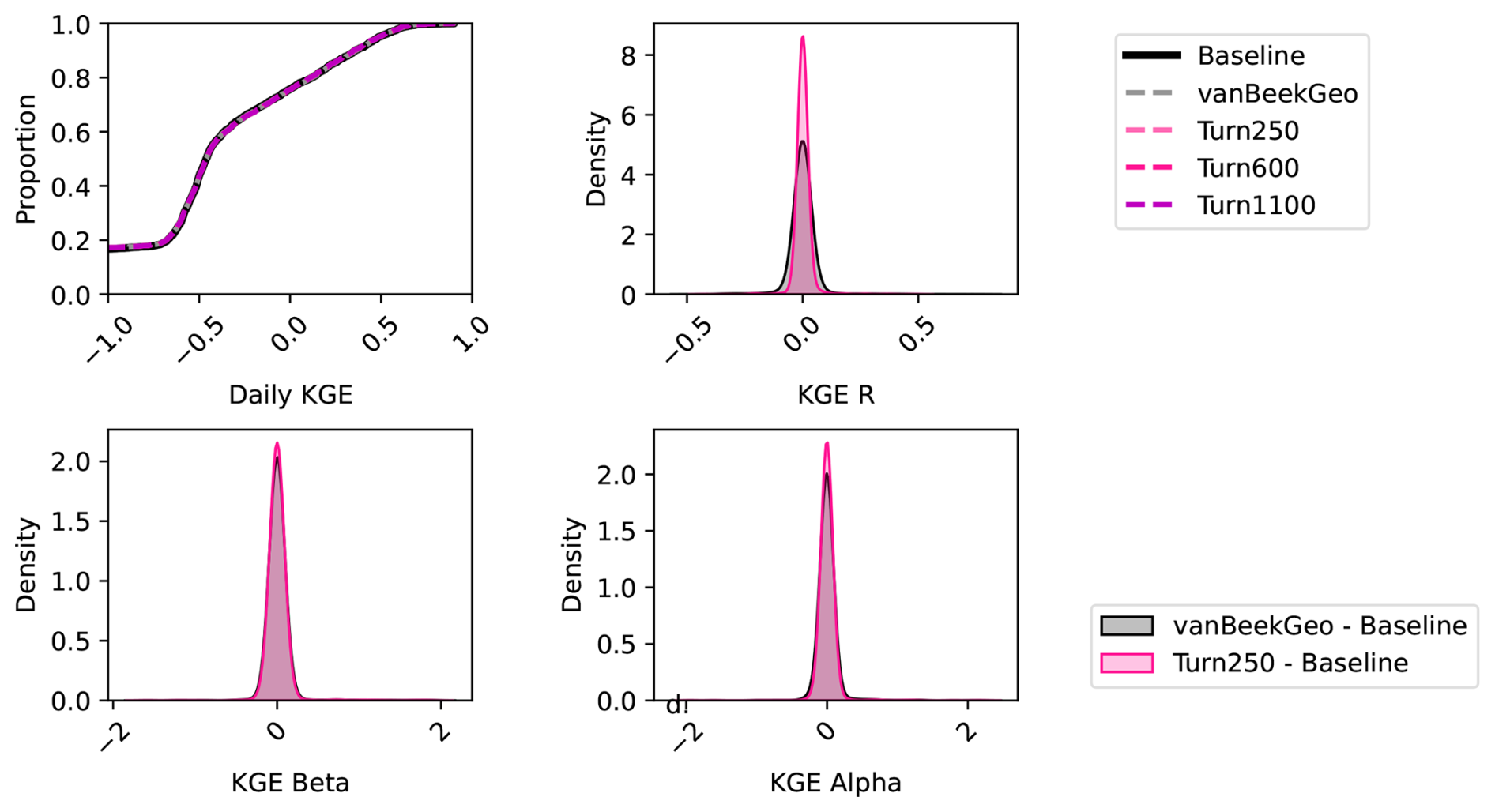
Figure A15Show the KGE, and KGE components of the models we used in our analysis for Fig. 5 in the manuscript without any zoom.
Table A2Performance metrics for the Clinton Lake Dam compared to the rest of the reservoirs within our analysis.
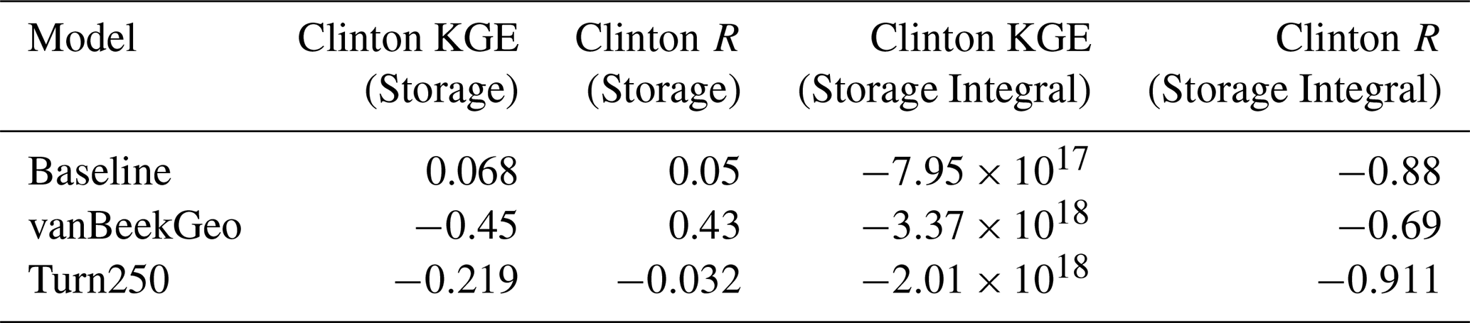
Table A3Performance metrics for the Koelnbrein Dam compared to the rest of the reservoirs within our analysis.
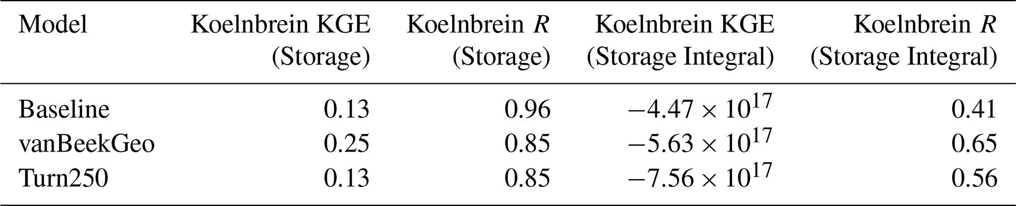
PCR-GLOBWB 2 is freely available at https://doi.org/10.5281/zenodo.17589689 (Steyaert et al., 2025) and all associated input data is currently available at https://doi.org/10.5281/zenodo.17590237 (Steyaert et al., 2025). All analysis and validation codes are available upon request.
All the modelled outputs in our analysis are available on YODA, a Utrecht Universiteit wide data repository at https://public.yoda.uu.nl/geo/UU01/F2UO5H.html (last access: 5 November 2025) and https://doi.org/10.24416/UU01-F2UO5H (Steyaert et al., 2025).
JCS, MB, and NW discussed and developed the research trajectory. JCS performed all the analysis and took point on the writing, while MB and NW provided valuable feedback in the writing and research phase. ES provided key support in developing the reservoir maps used in all of the analysis and supported the paper publication.
At least one of the (co-)authors is a member of the editorial board of Hydrology and Earth System Sciences. The peer-review process was guided by an independent editor, and the authors also have no other competing interests to declare.
Views and opinions expressed are those of the author(s) only and do not necessarily reflect those of the European Union or REA. Neither the European Union nor the granting authority can be held responsible for them.
Publisher's note: Copernicus Publications remains neutral with regard to jurisdictional claims made in the text, published maps, institutional affiliations, or any other geographical representation in this paper. While Copernicus Publications makes every effort to include appropriate place names, the final responsibility lies with the authors. Views expressed in the text are those of the authors and do not necessarily reflect the views of the publisher.
All authors are grateful for the European Union's Horizon EUROPE Research and Innovation Programme under Grant Agreement No. 101059264 (SOS-WATER – Water Resources System Safe Operating Space in a Changing Climate and Society) that financially supported this work. We are also grateful for the larger development team at Utrecht University that supports the model development of PCR-GLOBWB 2 and the two high performance computing clusters, without which this work would not be possible.
This research has been supported by the EU HORIZON EUROPE European Research Council (SOS-WATER – Water Resources System Safe Operating Space in a Changing Climate and Society (grant no. 101059264)).
This paper was edited by Yi He and reviewed by two anonymous referees.
Belletti, B., Garcia De Leaniz, C., Jones, J., Bizzi, S., Börger, L., Segura, G., Castelletti, A., Van De Bund, W., Aarestrup, K., Barry, J., Belka, K., Berkhuysen, A., Birnie-Gauvin, K., Bussettini, M., Carolli, M., Consuegra, S., Dopico, E., Feierfeil, T., Fernández, S., Fernandez Garrido, P., Garcia-Vazquez, E., Garrido, S., Giannico, G., Gough, P., Jepsen, N., Jones, P. E., Kemp, P., Kerr, J., King, J., Łapińska, M., Lázaro, G., Lucas, M. C., Marcello, L., Martin, P., McGinnity, P., O’Hanley, J., Olivo Del Amo, R., Parasiewicz, P., Pusch, M., Rincon, G., Rodriguez, C., Royte, J., Schneider, C. T., Tummers, J. S., Vallesi, S., Vowles, A., Verspoor, E., Wanningen, H., Wantzen, K. M., Wildman, L., and Zalewski, M.: More than one million barriers fragment Europe's rivers, Nature, 588, 436–441, https://doi.org/10.1038/s41586-020-3005-2, 2020. a
Biemans, H., Haddeland, I., Kabat, P., Ludwig, F., Hutjes, R. W. A., Heinke, J., von Bloh, W., and Gerten, D.: Impact of reservoirs on river discharge and irrigation water supply during the 20th century, Water Resources Research, 47, https://doi.org/10.1029/2009WR008929, 2011. a, b, c
Brunner, M. I. and Naveau, P.: Spatial variability in Alpine reservoir regulation: deriving reservoir operations from streamflow using generalized additive models, Hydrol. Earth Syst. Sci., 27, 673–687, https://doi.org/10.5194/hess-27-673-2023, 2023. a, b, c, d
Burek, P. and Smilovic, M.: The use of GRDC gauging stations for calibrating large-scale hydrological models, Earth Syst. Sci. Data, 15, 5617–5629, https://doi.org/10.5194/essd-15-5617-2023, 2023. a
Burek, P., Satoh, Y., Kahil, T., Tang, T., Greve, P., Smilovic, M., Guillaumot, L., Zhao, F., and Wada, Y.: Development of the Community Water Model (CWatM v1.04) – a high-resolution hydrological model for global and regional assessment of integrated water resources management, Geosci. Model Dev., 13, 3267–3298, https://doi.org/10.5194/gmd-13-3267-2020, 2020. a, b, c, d
Chalise, D. R., Sankarasubramanian, A., and Ruhi, A.: Dams and Climate Interact to Alter River Flow Regimes Across the United States, Earth's Future, 9, e2020EF001816, https://doi.org/10.1029/2020EF001816, 2021. a
Chen, T., Song, C., Luo, S., Ke, L., Liu, K., and Zhu, J.: Monitoring global reservoirs using ICESat-2: Assessment on spatial coverage and application potential, Journal of Hydrology, 604, 127257, https://doi.org/10.1016/j.jhydrol.2021.127257, 2022. a, b
Coerver, H. M., Rutten, M. M., and van de Giesen, N. C.: Deduction of reservoir operating rules for application in global hydrological models, Hydrol. Earth Syst. Sci., 22, 831–851, https://doi.org/10.5194/hess-22-831-2018, 2018. a
Cooley, S. W., Ryan, J. C., and Smith, L. C.: Human alteration of global surface water storage variability, Nature, 591, 78–81, 2021. a
Crétaux, J.-F., Abarca-del Río, R., Bergé-Nguyen, M., Arsen, A., Drolon, V., Clos, G., and Maisongrande, P.: Lake Volume Monitoring from Space, Surveys in Geophysics, 37, 269–305, https://doi.org/10.1007/s10712-016-9362-6, 2016. a
Di Baldassarre, G., Wanders, N., AghaKouchak, A., Kuil, L., Rangecroft, S., Veldkamp, T. I., Garcia, M., van Oel, P. R., Breinl, K., and Van Loon, A. F.: Water shortages worsened by reservoir effects, Nature Sustainability, 1, 617–622, 2018. a
Döll, P., Kaspar, F., and Lehner, B.: A global hydrological model for deriving water availability indicators: model tuning and validation, Journal of Hydrology, 270, 105–134, https://doi.org/10.1016/S0022-1694(02)00283-4, 2003. a
Döll, P., Fiedler, K., and Zhang, J.: Global-scale analysis of river flow alterations due to water withdrawals and reservoirs, Hydrol. Earth Syst. Sci., 13, 2413–2432, https://doi.org/10.5194/hess-13-2413-2009, 2009. a
Federal Institute of Hydrology: Global Runoff Data Centre, https://grdc.bafg.de/ (last access: 17 July 2023), 2020. a
Giachetta, E. and Willett, S. D.: A global dataset of river network geometry, Scientific data, 5, 1–10, 2018. a, b
Gleeson, T. and Wada, Y.: Assessing regional groundwater stress for nations using multiple data sources with the groundwater footprint, Environmental Research Letters, 8, 044010, https://doi.org/10.1088/1748-9326/8/4/044010, 2013. a
Grill, G., Lehner, B., Thieme, M., Geenen, B., Tickner, D., Antonelli, F., Babu, S., Borrelli, P., Cheng, L., Crochetiere, H., Ehalt Macedo, H., Filgueiras, R., Goichot, M., Higgins, J., Hogan, Z., Lip, B., McClain, M. E., Meng, J., Mulligan, M., Nilsson, C., Olden, J. D., Opperman, J. J., Petry, P., Reidy Liermann, C., Sáenz, L., Salinas-Rodríguez, S., Schelle, P., Schmitt, R. J. P., Snider, J., Tan, F., Tockner, K., Valdujo, P. H., Van Soesbergen, A., and Zarfl, C.: Mapping the world's free-flowing rivers, Nature, 569, 215–221, https://doi.org/10.1038/s41586-019-1111-9, 2019. a
Haddeland, I., Skaugen, T., and Lettenmaier, D. P.: Anthropogenic impacts on continental surface water fluxes, Geophysical Research Letters, 33, https://doi.org/10.1029/2006GL026047, 2006. a, b, c, d, e, f, g
Hanasaki, N., Kanae, S., and Oki, T.: A reservoir operation scheme for global river routing models, Journal of Hydrology, 327, 22–41, https://doi.org/10.1016/j.jhydrol.2005.11.011, 2006. a, b, c, d, e, f
Hoch, J. M., Sutanudjaja, E. H., Wanders, N., van Beek, R. L. P. H., and Bierkens, M. F. P.: Hyper-resolution PCR-GLOBWB: opportunities and challenges from refining model spatial resolution to 1 km over the European continent, Hydrol. Earth Syst. Sci., 27, 1383–1401, https://doi.org/10.5194/hess-27-1383-2023, 2023. a
Hosseini-Moghari, S.-M. and Döll, P.: The value of observed reservoir storage anomalies for improving the simulation of reservoir dynamics in large-scale hydrological models, Hydrol. Earth Syst. Sci., 29, 4073–4092, https://doi.org/10.5194/hess-29-4073-2025, 2025. a
Hou, J., Van Dijk, A. I. J. M., Renzullo, L. J., and Larraondo, P. R.: GloLakes: water storage dynamics for 27 000 lakes globally from 1984 to present derived from satellite altimetry and optical imaging, Earth Syst. Sci. Data, 16, 201–218, https://doi.org/10.5194/essd-16-201-2024, 2024. a, b, c, d, e, f, g, h, i, j, k, l, m, n
Kummu, M., de Moel, H., Ward, P. J., and Varis, O.: How Close Do We Live to Water? A Global Analysis of Population Distance to Freshwater Bodies, PLOS ONE, 6, 1–13, https://doi.org/10.1371/journal.pone.0020578, 2011. a
Lehner, B., Liermann, C. R., Revenga, C., Vörösmarty, C., Fekete, B., Crouzet, P., Döll, P., Endejan, M., Frenken, K., Magome, J., Nilsson, C., Robertson, J. C., Rödel, R., Sindorf, N., and Wisser, D.: High-resolution mapping of the world's reservoirs and dams for sustainable river-flow management, Frontiers in Ecology and the Environment, 9, 494–502, https://doi.org/10.1890/100125, 2011. a, b, c, d, e, f, g
Li, Y., Gao, H., Zhao, G., and Tseng, K.-H.: A high-resolution bathymetry dataset for global reservoirs using multi-source satellite imagery and altimetry, Remote Sensing of Environment, 244, 111831, https://doi.org/10.1016/j.rse.2020.111831, 2020. a, b, c
Li, Y., Zhao, G., Allen, G. H., and Gao, H.: Diminishing storage returns of reservoir construction, Nature Communications, 14, 3203, https://doi.org/10.1038/s41467-023-38843-5, 2023. a
Macian-Sorribes, H. and Pulido-Velazquez, M.: Inferring efficient operating rules in multireservoir water resource systems: A review, WIREs Water, 7, e1400, https://doi.org/10.1002/wat2.1400, 2020. a, b, c, d
Meigh, J., McKenzie, A., and Sene, K.: A grid-based approach to water scarcity estimates for eastern and southern Africa, Water resources management, 13, 85–115, 1999. a
Patterson, G. E., McIntyre, K. M., Clough, H. E., and Rushton, J.: Societal Impacts of Pandemics: Comparing COVID-19 With History to Focus Our Response, Frontiers in Public Health, 9, https://doi.org/10.3389/fpubh.2021.630449, 2021. a
Patterson, L. and Doyle, M.: Managing rivers under changing environmental and societal boundary conditions, Part 1: National trends and U.S. Army Corps of Engineers reservoirs, River Research and Applications, 35, https://doi.org/10.1002/rra.3418, 2019. a, b
Pietroniro, A., Fortin, V., Kouwen, N., Neal, C., Turcotte, R., Davison, B., Verseghy, D., Soulis, E. D., Caldwell, R., Evora, N., and Pellerin, P.: Development of the MESH modelling system for hydrological ensemble forecasting of the Laurentian Great Lakes at the regional scale, Hydrol. Earth Syst. Sci., 11, 1279–1294, https://doi.org/10.5194/hess-11-1279-2007, 2007. a, b
Potapov, P., Turubanova, S., Hansen, M. C., Tyukavina, A., Zalles, V., Khan, A., Song, X.-P., Pickens, A., Shen, Q., and Cortez, J.: Global maps of cropland extent and change show accelerated cropland expansion in the twenty-first century, Nature Food, 3, 19–28, https://doi.org/10.1038/s43016-021-00429-z, 2021. a
Rost, S., Gerten, D., Bondeau, A., Lucht, W., Rohwer, J., and Schaphoff, S.: Agricultural green and blue water consumption and its influence on the global water system, Water Resources Research, 44, https://doi.org/10.1029/2007WR006331, 2008. a
Salwey, S., Coxon, G., Pianosi, F., Singer, M. B., and Hutton, C.: National-Scale Detection of Reservoir Impacts Through Hydrological Signatures, Water Resources Research, 59, e2022WR033893, https://doi.org/10.1029/2022WR033893, 2023. a, b, c, d, e, f, g, h, i, j, k, l, m
Simeone, C. E., Hammond, J. C., Archfield, S. A., Broman, D., Condon, L. E., Eldardiry, H., Olson, C. G., and Steyaert, J. C.: Declining Reservoir Reliability and Increasing Reservoir Vulnerability: Long-Term Observations Reveal Longer and More Severe Periods of Low Reservoir Storage for Major United States Reservoirs, Geophysical Research Letters, 51, e2024GL109476, https://doi.org/10.1029/2024GL109476, 2024. a
Steyaert, J., Sutanudjaja, E., Bierkens, M. F. P., and Wanders, N.: Modelled outputs for ”A data derived workflow for reservoir operations (in global hydrologic models)”, YODA repository hosted by Utrecht University [data set], https://doi.org/10.24416/UU01-F2UO5H, 2024. a
Steyaert, J., Condon, L., Turner, S., and Voisin, N.: ResOpsUS, a dataset of historical reservoir operations in the contiguous United States, Scientific Data, 9, https://doi.org/10.1038/s41597-022-01134-7, 2022. a, b, c, d, e, f, g, h, i
Steyaert, J. C. and Condon, L. E.: Synthesis of historical reservoir operations from 1980 to 2020 for the evaluation of reservoir representation in large-scale hydrologic models, Hydrol. Earth Syst. Sci., 28, 1071–1088, https://doi.org/10.5194/hess-28-1071-2024, 2024. a, b, c, d, e, f, g, h
Steyaert, J., Sutanudjaja, E., Bierkens, M. F. P., and Wanders, N.: Data derived reservoir model implemented in PCR-GLOBWB2, Zenodo, https://doi.org/10.5281/zenodo.17589689, 2025. a
Steyaert, J., Sutanudjaja, E., Bierkens, M. F. P., and Wanders, N.: Operational inputs for PCR-GLOBWB2 data derived reservoir operations, Zenodo [data set], https://doi.org/10.5281/zenodo.17590237, 2025. a
Sutanudjaja, E. H., van Beek, R., Wanders, N., Wada, Y., Bosmans, J. H. C., Drost, N., van der Ent, R. J., de Graaf, I. E. M., Hoch, J. M., de Jong, K., Karssenberg, D., López López, P., Peßenteiner, S., Schmitz, O., Straatsma, M. W., Vannametee, E., Wisser, D., and Bierkens, M. F. P.: PCR-GLOBWB 2: a 5 arcmin global hydrological and water resources model, Geosci. Model Dev., 11, 2429–2453, https://doi.org/10.5194/gmd-11-2429-2018, 2018. a, b, c, d, e, f, g, h, i, j, k, l, m, n, o
Turner, S. W., Steyaert, J. C., Condon, L., and Voisin, N.: Water storage and release policies for all large reservoirs of conterminous United States, Journal of Hydrology, 603, 126843, https://doi.org/10.1016/j.jhydrol.2021.126843, 2021. a, b, c, d, e, f, g, h, i, j, k, l, m, n, o, p, q, r, s, t, u, v, w, x, y
van Beek, L. P. H., Wada, Y., and Bierkens, M. F. P.: Global monthly water stress: 1. Water balance and water availability, Water Resources Research, 47, https://doi.org/10.1029/2010WR009791, 2011. a, b, c, d, e, f, g, h
van Jaarsveld, B., Wanders, N., Sutanudjaja, E. H., Hoch, J., Droppers, B., Janzing, J., van Beek, R. L. P. H., and Bierkens, M. F. P.: A first attempt to model global hydrology at hyper-resolution, Earth Syst. Dynam., 16, 29–54, https://doi.org/10.5194/esd-16-29-2025, 2025. a, b
Voisin, N., Li, H., Ward, D., Huang, M., Wigmosta, M., and Leung, L. R.: On an improved sub-regional water resources management representation for integration into earth system models, Hydrol. Earth Syst. Sci., 17, 3605–3622, https://doi.org/10.5194/hess-17-3605-2013, 2013. a, b, c, d
Wada, Y., Wisser, D., and Bierkens, M. F. P.: Global modeling of withdrawal, allocation and consumptive use of surface water and groundwater resources, Earth Syst. Dynam., 5, 15–40, https://doi.org/10.5194/esd-5-15-2014, 2014. a
Wang, J., Walter, B. A., Yao, F., Song, C., Ding, M., Maroof, A. S., Zhu, J., Fan, C., McAlister, J. M., Sikder, S., Sheng, Y., Allen, G. H., Crétaux, J.-F., and Wada, Y.: GeoDAR: georeferenced global dams and reservoirs dataset for bridging attributes and geolocations, Earth Syst. Sci. Data, 14, 1869–1899, https://doi.org/10.5194/essd-14-1869-2022, 2022. a, b, c, d, e, f
Wang, Z., Jiang, L., Nielsen, K., and Wang, L.: Reservoir Filling Up Problems in a Changing Climate: Insights From CryoSat-2 Altimetry, Geophysical Research Letters, 51, e2024GL108934, https://doi.org/10.1029/2024GL108934, 2024. a, b
Wisser, D., Frolking, S., Hagen, S., and Bierkens, M. F. P.: Beyond peak reservoir storage? A global estimate of declining water storage capacity in large reservoirs, Water Resources Research, 49, 5732–5739, https://doi.org/10.1002/wrcr.20452, 2013. a, b
Yao, F., Livneh, B., Rajagopalan, B., Wang, J., Crétaux, J.-F., Wada, Y., and Berge-Nguyen, M.: Satellites reveal widespread decline in global lake water storage, Science, 380, 743–749, https://doi.org/10.1126/science.abo2812, 2023. a
Yassin, F., Razavi, S., Elshamy, M., Davison, B., Sapriza-Azuri, G., and Wheater, H.: Representation and improved parameterization of reservoir operation in hydrological and land-surface models, Hydrol. Earth Syst. Sci., 23, 3735–3764, https://doi.org/10.5194/hess-23-3735-2019, 2019. a, b, c, d, e, f
Zajac, Z., Revilla-Romero, B., Salamon, P., Burek, P., Hirpa, F. A., and Beck, H.: The impact of lake and reservoir parameterization on global streamflow simulation, Journal of Hydrology, 548, 552–568, https://doi.org/10.1016/j.jhydrol.2017.03.022, 2017. a, b, c
Zhang, X., Jiang, L., Kittel, C. M. M., Yao, Z., Nielsen, K., Liu, Z., Wang, R., Liu, J., Andersen, O. B., and Bauer-Gottwein, P.: On the Performance of Sentinel-3 Altimetry Over New Reservoirs: Approaches to Determine Onboard A Priori Elevation, Geophysical Research Letters, 47, e2020GL088770, https://doi.org/10.1029/2020GL088770, 2020. a
Zhao, G., Gao, H., Naz, B. S., Kao, S.-C., and Voisin, N.: Integrating a reservoir regulation scheme into a spatially distributed hydrological model, Advances in Water Resources, 98, 16–31, https://doi.org/10.1016/j.advwatres.2016.10.014, 2016. a, b, c