Evaluation of high-resolution snowpack simulations from global datasets and comparison with Sentinel-1 snow depth retrievals in the Sierra Nevada, USA

The spatial distribution of mountain snow water equivalent (SWE) is key information for water management. We implement a tool to simulate snowpack properties at high resolution (100 m) by using only global datasets of meteorology, land cover and elevation. The meteorological data are obtained from ERA5, which makes the method applicable in near real time (5 d latency). We evaluate the output using 49 SWE maps derived from airborne lidar surveys in the Sierra Nevada. We find very good agreement at the catchment scale using uncalibrated lapse rates. Larger biases at the model grid scale are especially evident at high elevation but do not alter the catchment-scale snow mass accuracy. We additionally compare the simulated snow depth to Sentinel-1 retrievals and find a similar accuracy with respect to synchronous airborne lidar surveys. However, Sentinel-1 snow depth products are sparse and often masked during the melt season, whereas ERA5–SnowModel provides a spatially and temporally continuous SWE.

1 Introduction

Many populated regions with dry summers and wet winters depend on mountain snow for water supply (Mankin et al., 2015; Sturm et al., 2017; Viviroli et al., 2020). Understanding the catchment-scale seasonal snow storage before and during the melt season is key to optimizing water use between hydropower production, crop irrigation and freshwater supply. In addition, an accurate prediction of the timing and magnitude of the snowmelt runoff is bound by our ability to characterize the spatial distribution of mountain snow before the melt season (Freudiger et al., 2017).

Despite its hydrological significance, snow water equivalent (SWE) remains poorly monitored in many mountainous regions, especially outside North America and Europe. In situ measurements are often too sparse considering the spatial variability of mountain snow (Fayad et al., 2017). To cope with this issue, airborne measurement campaigns are now routinely used in the western USA to measure snow depth, but their cost remains prohibitive in other regions (Painter et al., 2016). Meanwhile, several approaches have emerged to retrieve mountain snow depth using satellite remote sensing (e.g., Pléiades, ICESat-2 and Sentinel-1). Pléiades very-high-resolution stereoscopic images can be used to generate snow depth images by differencing two digital elevation models. However, this approach is limited to small regions (Marti et al., 2016). ICESat-2 lidar altimetry has the potential to provide snow depth data at a global scale but with sparse sampling (Deschamps-Berger et al., 2023). Sentinel-1 has been used to derive snow depth at 1 km resolution in the Northern Hemisphere (Lievens et al., 2019) and 500 m resolution over the European Alps (Lievens et al., 2022). This method, which is based on an empirical change detection method applied to the cross-polarization ratio, is limited to dry snow conditions and therefore does not allow monitoring of the snowpack during the melt season. However, it offers global and spatially continuous coverage, which is a key advantage with respect to the other approaches. All the above remote sensing approaches require an estimation of snow density to obtain the SWE, but it has been established that snow depth explains most of the SWE variance (Guyennon et al., 2019; López-Moreno et al., 2013; Sturm et al., 2010; Bormann et al., 2013).

Another approach to estimating mountain SWE distribution is to use a snowpack model, but the challenge then lies in obtaining accurate meteorological forcing (Günther et al., 2019; Raleigh et al., 2016). To cope with the lack or sparsity of in situ meteorological measurements, one solution is to use atmospheric model outputs as forcing data. In particular, climate reanalyses can provide long-term hourly meteorological data at a global scale. Climate reanalyses are also becoming increasingly accurate (Hersbach et al., 2020) with advances in atmospheric and land surface modeling and the assimilation of a growing dataset of in situ and remote sensing observations. These reanalyses have also seen notable progress in recent years in terms of latency. For example, the preliminary ERA5 reanalysis provided by the European Centre for Medium-Range Weather Forecasts has a short latency of 5 d (whereas it was 2–3 months with the previous ERA-Interim version). This preliminary product only rarely deviates from the fully quality-checked final product that is released 2 months later (Hersbach et al., 2020). This timely product can fulfill the need for up-to-date meteorological forcing information. However, reanalyses cannot be used directly to force a mountain snowpack model because the grid cell size is too coarse (approximately 30 and 50 km for ERA5 and MERRA-2 respectively), which creates large biases in the computed SWE (Wrzesien et al., 2019; Liu et al., 2022).

To address the mismatch in spatial resolution between reanalysis datasets and snow distribution, previous studies used downscaling algorithms based on a digital elevation model before running a snowpack model on a finer grid (Armstrong et al., 2018; Baba et al., 2018; Billecocq et al., 2024; Mernild et al., 2017; Weber et al., 2021). This approach enables estimation of high-resolution SWE and snow depth without ground data. For example, Mernild et al. (2017) and Baba et al. (2018) studied the snowpack properties over large and ungauged regions in the Andes and High Atlas mountain ranges using the MicroMet/SnowModel package (Liston et al., 2020; Liston and Elder, 2006a, b). The evaluation of these simulations relied on in situ observations or remote sensing snow cover areas. Weber et al. (2021) used 10 years of snow depth measurements from two automatic weather stations to assess their simulations in the Research Catchment Zugspitze (12 km²). Mernild et al. (2017) used 13 years of MODIS data over the Andes Cordillera ($\sim \mathrm{9}\times {\mathrm{10}}^{\mathrm{6}}$ km²) along with 4 km grid maps of snow depth that were reconstructed from in situ observations. Baba et al. (2018) used 18 years of MODIS data to assess simulations in the High Atlas of Morocco, snow depth at a single automatic weather station, precipitation at three meteorological stations and river discharge of the Ourika catchment (503 km²). However, in situ data are sparse and MODIS snow cover area does not allow a thorough evaluation of the model ability to capture snow mass across the landscape.

In this study, we focus on the Tuolumne River catchment in the Sierra Nevada, USA (Fig. 1). Since 2013, this site has been surveyed regularly by the Airborne Snow Observatory (ASO) to determine snow depth and SWE. The ASO dataset on the Tuolumne River catchment is the densest time series of high-resolution snow depth (3 m) and SWE (50 m) maps publicly available at this scale (1100 km²) in the world. The dataset contains 49 surveys and spans several years with contrasted climatic conditions, including California's most severe drought in the last 1200 years during 2012–2014 (Griffin and Anchukaitis, 2014) and the “snowpocalypse” 2016–2017 winter that was characterized by near-record snow accumulation (Painter et al., 2017). We leverage this observational dataset to evaluate a new processing pipeline which generates gridded SWE and snow depth with a resolution of 100 m from ERA5 or ERA5-Land. This pipeline, inspired by previous works (Baba et al., 2018; Mernild et al., 2017), is a wrapper around the MicroMet/SnowModel code. It was designed to work with global meteorological forcing datasets. As such, the workflow can generate high-resolution snow cover simulations in any region of interest across the globe from 1940 up to the present, with any resolution between 1 and 200 m (Liston and Elder, 2006b). Furthermore, we compare the output of this pipeline with the more direct approach of Sentinel-1 snow depth on dates matching the ASO measurements.

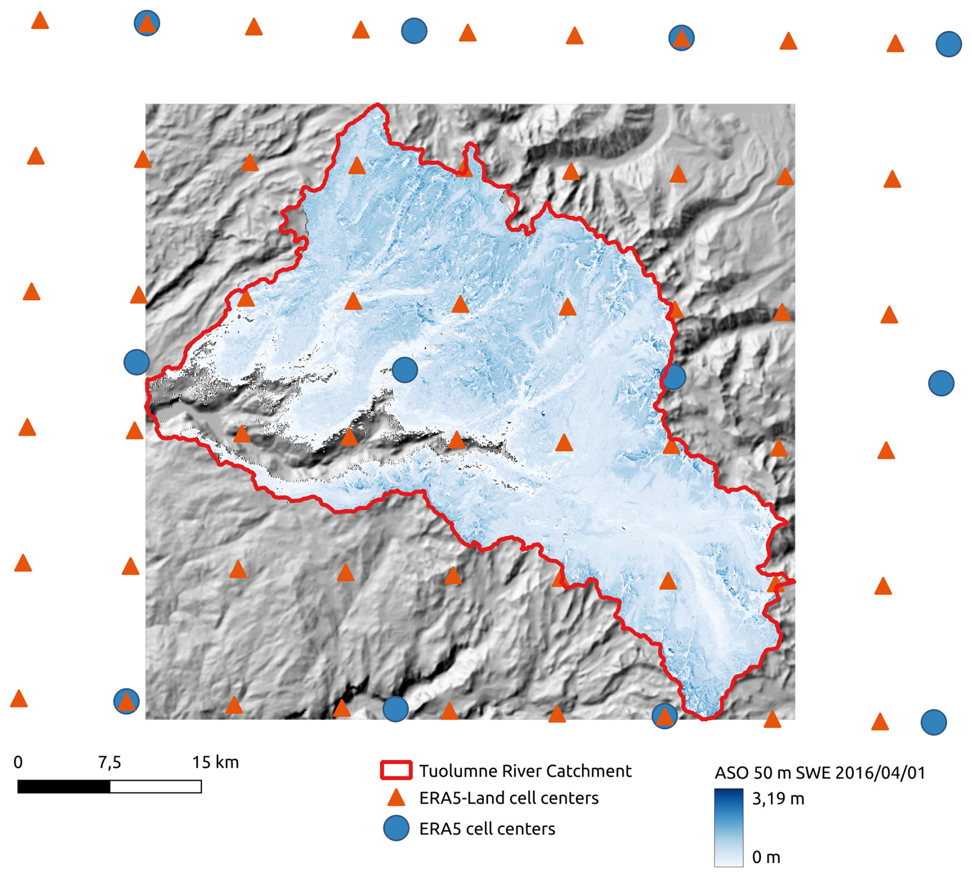
Figure 1 Map representing the SWE variability measured by the ASO, along with ERA5 and ERA5-Land cell centers and the Tuolumne River catchment border overlaying the DEM hillshade.

2 Data and methods

2.1 Data

We used two reanalyses in this study, ERA5 and ERA5-Land. ERA5 is a reanalysis of the global climate and weather since 1940, with a 0.25° resolution (approximately 30 km). It provides hourly atmospheric, oceanic and land surface variables computed with a global model and improved by the assimilation of multiple in situ and remote sensing datasets (Hersbach et al., 2020). ERA5-Land is produced by recomputing ERA5-Land variables at finer resolution using a downscaled meteorological forcing (Muñoz Sabater, 2019). It delivers these variables at a global scale at a 0.1° resolution from 1950 to the present. As mentioned above, preliminary versions of ERA5 and ERA5-Land are distributed with a short latency of 5 d. These datasets are freely available from the Copernicus Climate Change Service (C3S) and can be queried via their application programming interface (with tutorials that can be found on their website: Retrieving data – Climate Data Store Toolbox 1.1.5 documentation; CDS, 2025). We focused on ERA5 here as we found that it yielded slightly better results than MERRA-2 in a previous case study using the same approach (Baba et al., 2021). In addition, the latency of MERRA-2 is 3 weeks, which may be too long for operational water resource applications. To run the model (see Sect. 2.2.1), we also used the 30 m Copernicus DEM (CDS, 2023) and the 100 m Copernicus land cover (Buchhorn et al., 2020).

We obtained Sentinel-1 snow depth between 2016 and 2019 from the C-SNOW repository (C-SNOW, 2022). Sentinel-1 C-band backscatter observations were used to derive ∼1 km resolution snow depth using empirical change detection (Lievens et al., 2019). This product has a revisit time of approximately 3 d over the Tuolumne River catchment during winter but provides almost no data in spring because the algorithm is considered to be invalid when the snowpack contains liquid water. When the snowpack is wet, there is higher absorption and reflection of the microwave signal emitted by Sentinel-1, which greatly decreases the performance of the C-SNOW algorithm (Lievens et al., 2019; Tsai et al., 2019).

For the evaluation of model outputs and Sentinel-1 products, we used 49 SWE and snow depth maps collected between 2013 and 2019 by the ASO. The ASO acquires hyperspectral data for snow albedo and lidar data for snow depth and computes SWE as a derived product (Painter et al., 2016). Snow depth is available at 3 m resolution, while SWE has 50 m resolution. The reported accuracy of the 3 m snow depth products is 0.08 m (Painter et al., 2016), and from spatially intensive sampling the reported accuracy for the 50 m snow depth products is <0.01 m (Painter et al., 2016; Fig. 15). There are no published references for the 50 m SWE product. However, Raleigh and Small (2017) estimated an uncertainty in the modeled density of 48 kg m⁻³ in the Tuolumne River basin. This uncertainty can be regarded as a conservative estimate as in situ measurements of snow density are also used by the ASO to adjust their density model (Painter et al., 2016). Therefore, for a 1 m deep snowpack and an uncertainty in the snow density of 50 kg m⁻³, we estimate the uncertainty of the 50 m SWE products to be 0.05 m w.e. (meters of water equivalent).

2.2 Methods

2.2.1 SnowModel

SnowModel is designed to simulate snow evolution on a high-resolution grid (1 to 200 m increments) and at a time step from 1 min to 1 d (Liston et al., 2020; Liston and Elder, 2006a). It is separated into four submodels: (i) MicroMet redistributes meteorological forcings (air temperature, relative humidity, wind speed and direction, precipitation, solar radiation, longwave radiation and surface pressure) to the target simulation grid (Liston and Elder, 2006b). (ii) EnBal computes the snow surface energy balance. (iii) SnowPack computes the snow density and snow depth. (iv) SnowTran-3D computes the blowing snow sublimation and snow redistribution due to wind transport (Liston et al., 2007). SnowModel accounts for the vegetation effects on the snow cover, such as coniferous forests or grassland, for the grid cell vegetation type. MicroMet was originally designed to interpolate station data on a regular grid. Here, a climate reanalysis grid cell is considered a virtual station located at the grid cell center.

2.2.2 Model input

We developed a tool to automatically prepare SnowModel input files from ERA5 and ERA5-Land data and run the simulations. This tool uses a DEM of the region of interest as input along with the start and end of the simulation period. We let the user specify the DEM because it is used to define the model grid, which is the main control of the computation time. Here we used the 30 m Copernicus orthometric DEM that we extracted and resampled to a World Geodic System 1984, Universal transverse Mercator zone 11N (WGS84 UTM 11N) grid at 100 m resolution using the bilinear method over a region covering the Tuolumne River catchment. The simulation period was set to September 2012–August 2019 and spans 7 years of snowpack dynamics. Using the Climate Data Store Application Program Interface, our tool downloads ERA5 or ERA5-Land hourly meteorological data (2 m temperature, 2 m dew point temperature, precipitation, and 10 m wind eastward and northward components) over the region of interest given by the DEM bounding box extended to the adjacent ERA5 and ERA5-Land neighboring cells (∼30 km and 11 km, respectively). Once downloaded, the meteorological data are processed to match SnowModel and MicroMet input formats and units. ERA5-Land precipitation is provided as daily cumulative values and is therefore converted into an hourly precipitation rate. Wind components (u and v) are converted into wind speed and direction (0–360° N). The dew point temperature is converted into relative humidity using Buck's equation (Buck, 1981), the same equation that is used in MicroMet. The elevations of ERA5 and ERA5-Land cells are determined from the global geopotential file that is first interpolated onto the model grid with a bilinear algorithm. The tool also resamples the Copernicus land cover map on the model grid using the mode-resampling algorithm (GDAL/OGR contributors, 2024). We built a correspondence table to remap the Copernicus land cover classes to the SnowModel land cover classification (see Table A1). We set all SnowModel parameters (the curvature length scale, curvature and wind slope weights, minimum wind speed, precipitation schemes for downscaling or for rain–snow fractions, subcanopy radiation schemes and various thresholds for wind transport calculations) to the default values (see the parameter file snowmodel.par in the “Code availability” section). A simple parameterization of the albedo is used with a constant value of 0.8 under dry conditions, whereas albedo values for melting snow cover are set according to land covers (Liston et al., 2020). We used the default monthly temperature lapse rates and precipitation factors which adjust the precipitation values to the elevation of the model grid. This tool is implemented in Python. The source code and more detailed documentation are available in the “Code availability” section.

2.2.3 Comparison with the ASO SWE

We resampled the ASO SWE (n=49 surveys) to the model grid, which has a resolution of 100 m. The resampling was done using the weighted average of all valid contributing pixels (GDAL/OGR contributors, 2024). We also created a validity mask to select cells in the Tuolumne River catchment that were always observed by the ASO during this period (some regions were not always available, representing 2.5 % of the catchment area). ASO data and ERA–SnowModel outputs were averaged over the valid cells to compute the temporal evolution of the catchment-mean SWE. Then, we analyzed the spatially distributed residuals in the catchment for each observation date of a dry year (2014–2015), a wet year (2016–2017) and an average year (2015–2016). We used the validity-masked SWE maps to subtract the ASO observations from the ERA–SnowModel output. A positive bias means the simulated SWE is higher than the observations.

Additionally, we extracted ERA5 and ERA5-Land daily SWE over the Tuolumne River catchment and computed the catchment-scale SWE using an area-weighted average (i.e., each SWE value was weighted by the fraction of the grid cell area within the catchment). Since these SWE products have very coarse resolutions of approximately 31 and 9 km (Figs. 1 and 2), we did not use them to analyze the residual distribution as above.

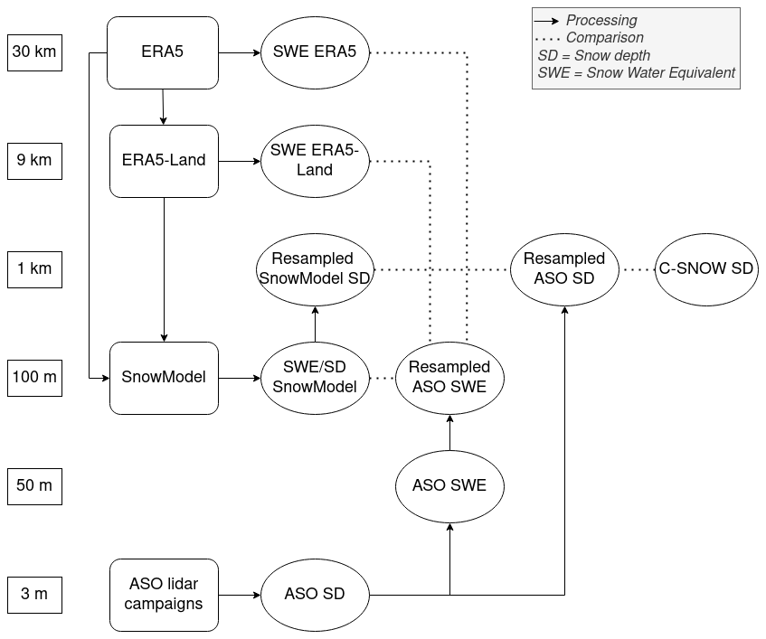
Figure 2 Summary of the different data sources with their spatial resolutions. The arrows represent a process and the dotted lines the comparison between the different data.

2.2.4 Comparison with Sentinel-1 snow depth

Over the entire study period, we identified three matchup dates for which we have both ASO and Sentinel-1 snow depth observations with a minimum coverage of 60 % of the catchment area. On these dates, the snow depths given by the ASO, Sentinel-1 and ERA–SnowModel were resampled to a common 1 km UTM grid. We applied another validity mask for cells where the snow depth was not always available to all three snow depth datasets (representing 8.5 % of the catchment changed to missing data). The missing values in the 3 m ASO dataset are propagated at the 1 km validity mask. This decreases the number of observations but ensures that the resampled 1 km snow depth maps are not biased by the spatial distribution of invalid pixels in the 3 m ASO snow depth dataset. We computed the distributed residuals by subtracting the ASO snow depth from both SnowModel simulations and Sentinel-1 data. For each date, we averaged the residuals to compute the mean bias, and we computed the standard deviation of the error. We also computed the RMSE over the catchment for each date.

3 Results

3.1 Comparison with the ASO SWE

Figure 3 shows the temporal evolution of the catchment-scale SWE from ASO observations and SnowModel simulations forced with ERA5 and ERA5-Land. There is very good agreement between the observations and both simulations, with an overall correlation of 0.99 for both ERA5 and ERA5-Land–SnowModel simulations (with 49 observation dates). First, both simulations capture the large interannual variability of SWE in the Tuolumne River catchment during the study period. The observed annual peak SWE ranges from 0.11 m in 2015 to 1.27 m in 2017, while the SnowModel simulations range from 0.17 to 1.19 m with ERA5 and from 0.12 to 1.24 m with ERA5-Land during the same years (but on different dates). In addition, the model reproduces the seasonal evolution of SWE, with an annual RMSE ranging from 0.03 to 0.13 m. The catchment-scale SWE accumulation in the ERA5–SnowModel simulations is captured well. We note an underestimation of the snow ablation rates in late spring, which caused a delay in the date of complete meltout of a few days (2013) to approximately 1 month (2019). This issue is mostly evident in 2016–2017 since the ablation rates are insufficient for reaching complete removal of the snowpack in August as observed by the ASO. Interestingly, we also note that ERA5-Land without resampling almost always reports the lowest RMSE at the catchment scale, though at 0.1° the distribution of the snow is not represented well.

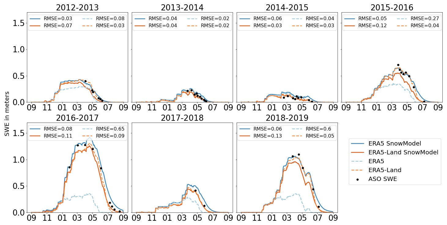
Figure 3 Temporal evolution of the Tuolumne River catchment SWE for 7 hydrological years from 2012 to 2019. The legend indicates the RMSE between the simulated SWE and the ASO SWE for each year.

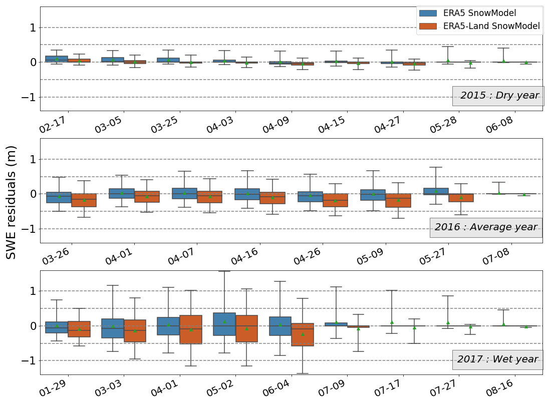
Figure 4 Distribution of the residuals between the SnowModel-simulated SWE and the ASO SWE at 100 m resolution in the Tuolumne River catchment (m w.e.) for 3 contrasted hydrological years. The filled boxes represent the interquartile range, the whiskers show the 5th to 95th percentiles, the line in each box represents the median of the distribution and the green triangle shows the mean.

To go beyond this coarse catchment-scale diagnostic (1100 km²), we also analyzed the distribution of the residuals at the pixel scale (0.01 km²). We computed a map of the RMSE using all 49 validation dates we have between 2013 and 2019; 10 % of the cells in this map have an RMSE above 0.5 m w.e. Figure 4 shows the distribution of the residuals for every date with the ASO observations for 3 contrasted hydrological years. The spread of the residuals is shown with the interquartile range (i.e., the difference between the 25th and 75th percentiles) inside the colored boxes and with the 5th to 95th percentiles inside the whiskers. This figure indicates that the spread of the residuals increases with the mean SWE depth. For the dry year, the interquartiles of the SnowModel SWE residuals for ERA5 and ERA5-Land do not exceed 0.17 and 0.09 m w.e., respectively. For the average year, the interquartiles reach 0.31 and 0.38 m w.e., and for the wet year 2017 they peak at 0.64 and 0.82 m w.e., respectively.

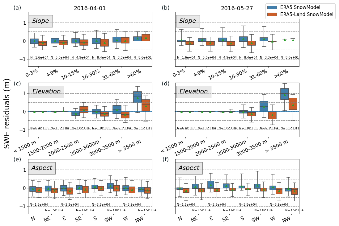
Figure 5 Distribution of the residuals between the SnowModel-simulated SWE and the ASO SWE at 100 m resolution in the Tuolumne River catchment (m w.e.) on 1 April 2016 (a, c, e) and 27 May (b, d, f), stratified by slope (%), elevation (m a.s.l.) and aspect (° N). The whiskers show the 5th to 95th percentiles, the line in each box represents the median of the distribution and the green triangle shows the mean. The slope, elevation and aspects have been calculated using the DEM at 100 m resolution.

Figure 5 shows the distribution of the residuals for two dates (1 April and 27 May 2016) by slope, elevation and aspect. We aimed to distinguish the model performance in terms of accumulation and ablation processes to better separate the sources of uncertainties in future studies. Therefore, we selected a date before the melting season (1 April 2016) and a date near the end of the melting season (27 May 2016). The interquartile of the error distribution never exceeds 0.41 m w.e. in the slope or aspect categories but peaks at 0.67 m w.e. in the highest-elevation band on 1 April for the simulations forced with ERA5-Land.

3.2 Comparison with Sentinel-1 snow depth

Between 2016 and 2019, there are three dates for which we have both Sentinel-1 and ASO snow depth data. Figure 6 presents snow depth maps of the Tuolumne River catchment at 1 km resolution with Sentinel-1, ASO and ERA5–SnowModel data. Some pixels are not always observed with ASO data, and these missing values are propagated at 1 km resolution (if there is at least one missing value among the contributing pixels, a missing value is attributed to the target 1 km cell). The same mask is applied to the SnowModel simulations and the Sentinel-1 data. Additional missing values are observed on the Sentinel-1 snow depth maps. Therefore, the statistics of Fig. 7 are not computed in the exact same area. We chose to take all possible data into account.

Figure 6 Snow depth maps at 1 km resolution with Sentinel-1, ASO and ERA5–SnowModel data.

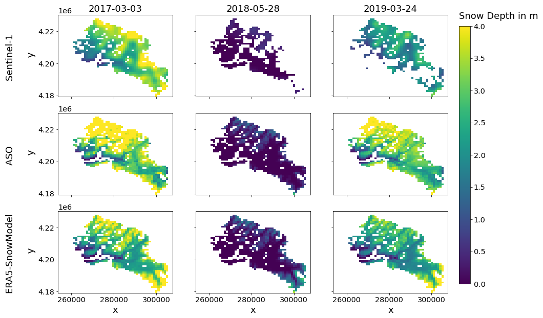
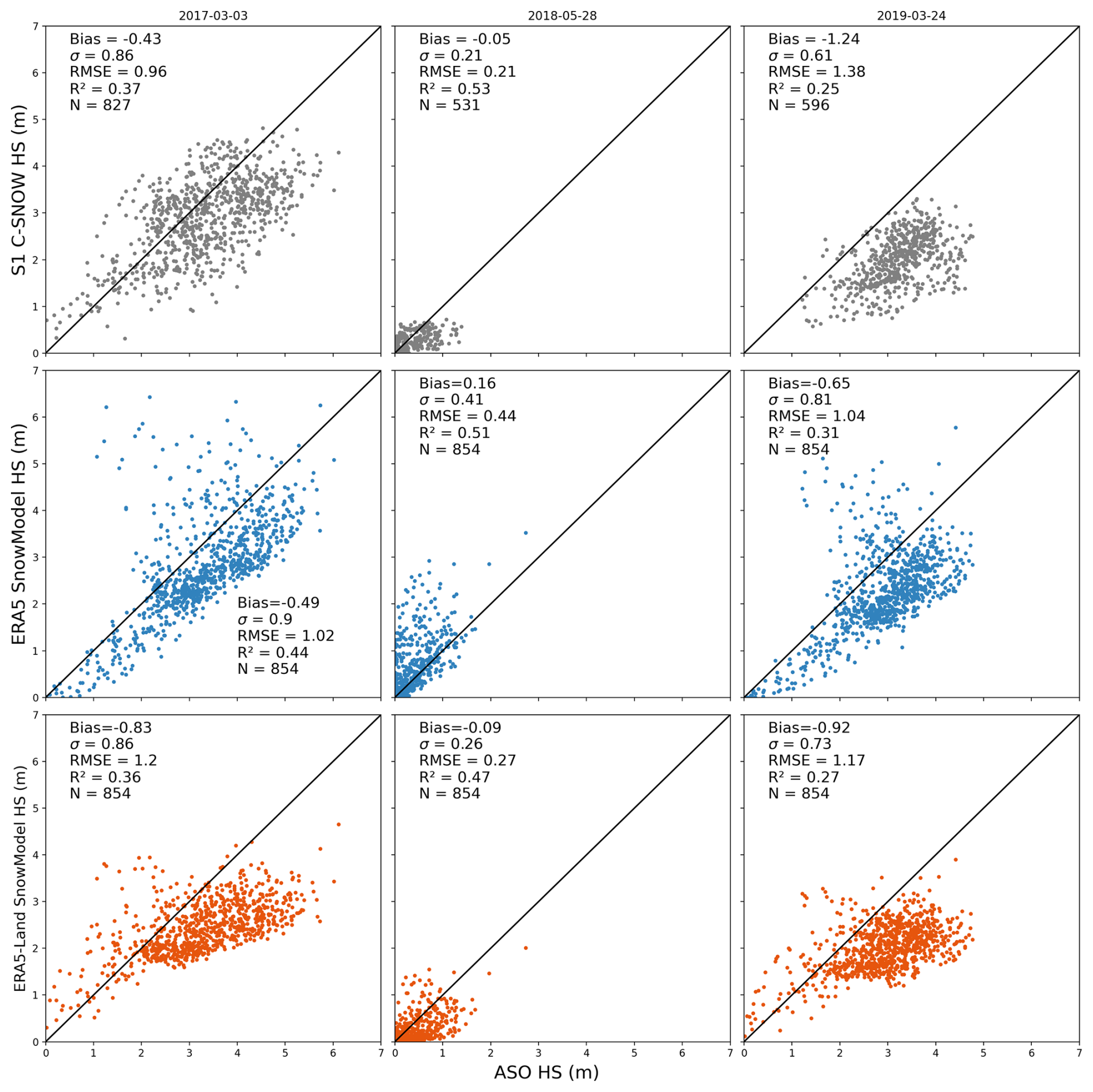
Figure 7 Scatterplots representing the observed and SnowModel-simulated snow depth data as a function of ASO snow depth data, with a 1 : 1 line in black. All data are resampled at 1 km resolution. N is the number of values in each plot.

Figure 7 shows the Sentinel-1-observed and SnowModel-simulated snow depth compared to the ASO-observed snow depth, resampled to 1 km resolution. On 3 March 2017, Sentinel-1 has the lower bias (−0.43 m), standard deviation (0.86 m) and RMSE (0.96 m). These statistics are close to the ERA5–SnowModel simulations (−0.49, 0.9 and 1.02 m, respectively), while the ERA5-Land–SnowModel simulations have a greater bias (−0.83 m) and RMSE (1.2 m) with a comparable standard deviation (0.86 m). On the second date, 1 May 2018, Sentinel-1 still performs best, with a bias of −0.05 m and a standard deviation and RMSE both equal to 0.21 m. On this date, ERA5-Land–SnowModel simulations are similar to Sentinel-1, with a bias of −0.09 m, a standard deviation of 0.26 m and an RMSE of 0.27 m, while ERA5–SnowModel simulations underperform with a 0.16 m bias, a 0.41 m standard deviation and a 0.44 m RMSE. Finally, on 24 March 2019, the data closer to the ASO snow depths seem to be the ERA5–SnowModel simulations with a bias of −0.65 m, a standard deviation of 0.81 m and an RMSE of 1.04 m. Sentinel-1 data have the highest bias (−1.24 m) and RMSE (1.38 m) but the lowest standard deviation (0.61 m). ERA5-Land–SnowModel simulations also have a high bias (−0.92 m) and RMSE (1.17 m), with a standard deviation of 0.73 m. We see an underestimation of the snow depth above 2 m with Sentinel-1 in 2017 and 2019, which is very clear for 2019, when the mean bias is highest with a relatively low standard deviation. In 2018, both the ASO and Sentinel-1 observed really low snow depths (<1 m), but there is still a negative bias (−0.05 m) in the Sentinel snow depth distribution. With the ERA5–SnowModel simulations, most of the distribution is centered around a negative bias that underestimates the snow depth in 2017 and 2019. We note several cells with a high positive error. In 2018, the situation is reversed: most of the snow depth estimated with ERA5–SnowModel is overestimated. Finally, the simulations with ERA5-Land seem to have a cap at 4 m snow depth in 2017 and 2019, with a declining accuracy with the ASO snow depth starting at 2 m. In 2018, the ERA5-Land–SnowModel simulations mostly underestimate the snow depths.

4 Discussion

Downscaling ERA5 forcing is critical to obtaining a realistic SWE in the Tuolumne River catchment and is sufficient to remove the strong negative bias that is otherwise present in the original ERA5 SWE (Fig. 3). The use of this pipeline for long simulation periods could also bypass the discontinuities in the ERA5 SWE (Urraca and Gobron, 2023), which are caused by snow capping in the data assimilation code and the arrival of new snow depth data available for assimilation. The main effect of the downscaling is a better representation of the air temperature distribution and therefore a better representation of the solid precipitation fraction. Then, the performance of the SnowModel-simulated SWE largely relies on ERA5 precipitation. Our results suggest that the winter precipitation is represented well by ERA5 over the Sierra Nevada, in agreement with previous studies highlighting the good performances of ERA5 precipitation, especially in the extratropical regions (Lavers et al., 2022). We find an overestimation of snow accumulation at high elevations, which only occurs above 3000 m a.s.l. In the study domain, the maximum elevations of the ERA5 and ERA5-Land grid cells are 2654 and 3100 m, respectively. Hence the overestimation shown in Fig. 5 is likely due to the extrapolation of ERA5 precipitation by MicroMet. MicroMet uses monthly coefficients to adjust precipitation with elevation. These coefficients were derived from a large precipitation gauge dataset in western North America that included the Tuolumne River catchment (Liston and Elder, 2006b). As a result, they only represent a first-order variation of precipitation with elevation and may only introduce large biases in areas whose fine-scale elevations (i.e., at the scale of the 100 m grid) deviate substantially from the ERA5 grid cell elevation. A possible source of error in high-elevation regions is the lack of gravitational transport in SnowModel. High-elevation and steep slopes are prone to avalanches, thereby reducing the accumulated snow in these areas during the winter season (Quéno et al., 2024). However, we did not find a clear correlation between the terrain slope and the model error (Fig. 5). Slopes above 15 % have a slightly wider error distribution, but the mean absolute biases remain below 0.10 m w.e. for both simulations. We also verified the residuals distribution by average slope classes computed from a 3 m resolution slope raster (computed from the ASO snow-off lidar DEM) and found similar results (see Fig. A1). Hence, we do not see clear evidence that the lack of gravitational transport is the main cause of the high-elevation biases. Another significant source of uncertainty is related to the albedo parameterization in SnowModel. The deposition of light-absorbing particles like dust can reduce albedo and therefore increase melt, especially at high elevation (Skiles et al., 2018; Dumont et al., 2020). This might explain the relative increase in the SWE bias between 1 April and 27 May at all elevations above 2500 m (Fig. 5).

At the catchment scale we do not find a clear difference between ERA5–SnowModel and ERA5-Land–SnowModel outputs. This suggests that the details of the downscaling scheme are not the primary factors in the simulation performance. However, there is a deviation between both simulations at high elevation. As shown in Fig. 5, the downscaling of ERA5 creates a strictly increasing bias with elevations above 2500 m, whereas ERA5-Land creates a more complex bias that is negative between 2000 and 3000 m and becomes positive above 3500 m. This more complex bias distribution reflects the fact that the output of the ERA5-Land–SnowModel pipeline is the result of two downscaling schemes (first ERA5 to ERA5-Land and then ERA5-Land to 100 m using MicroMet; Fig. 2). ERA5-Land atmospheric variables are generated by linear interpolation of their ERA5 counterparts. ERA5-Land air temperature and humidity are also adjusted using the grid cell elevation and a daily lapse rate derived from the ERA5 lower-tropospheric temperature vertical profile (Dutra et al., 2020). This is similar to the MicroMet algorithm. However, there are several differences. In particular, the air temperature downscaling scheme in ERA5-Land is based on a daily environmental lapse rate derived from ERA5 lower-tropospheric temperature vertical profiles (Muñoz Sabater, 2019), whereas MicroMet lapse rates are fixed by month. Unlike ERA5-Land, MicroMet also adjusts the precipitation rates using a function of elevation (Liston and Elder, 2006b). This is the cause of the nonmonotonic evolution of the SWE bias by elevation from ERA5-Land–SnowModel. In future applications we will favor ERA5 instead of ERA5-Land to avoid conflicting processes in the downscaling of atmospheric variables. This will make it easier to adjust the precipitation correction factors from local data. Using ERA5 is also more practical as it significantly reduces the download time, computing cost and memory usage of our pipeline.

In Fig. 3, we note the very good performance of ERA5-Land SWE at the catchment scale despite its coarse scale (9 km resolution). This result is in line with Muñoz-Sabater et al. (2021), who found better performances of ERA5-Land than ERA5 between 1500 m and 3000 m a.s.l. because 68 % of the Tuolumne River catchment is in this elevation band. Shao et al. (2022) found a similar accuracy of the ERA5-Land SWE dataset, with an RMSE below 0.04 m w.e. in regions north of 45° N. This evaluation was performed using point-scale in situ measurements over large flat regions and not in complex mountain terrain like the Tuolumne River basin, where the high spatial variability of SWE makes such evaluations more challenging (Mortimer et al., 2024). Overall, the performance of ERA5-Land SWE needs to be consolidated in other regions and ideally over larger domains of mountainous areas. Previous studies suggested that a resolution below 500 m is required to properly simulate the snowpack distribution (Baba et al., 2019; Bair et al., 2023). In addition, the ERA5-Land resolution does not meet the essential climate variable requirements set by the World Meteorological Organization for SWE (the goal is 500 m resolution) (WMO, 2022).

Regarding Sentinel-1, Fig. 7 suggests that the snow depth is captured well by the C-SNOW algorithm at 1 km resolution. Although we are interested in SWE and not snow depth, the ASO program has shown that useful SWE products can be derived from remotely sensed snow depth when combined with in situ measurements and modeled snow density (Painter et al., 2016). Figure 7 shows that the Sentinel-1 snow depth dataset agrees moderately with the spatial variability inside the catchment, although we note a slight underestimation for all three dates, before the melting period (2017 and 2019) and after it (2018). There is no clear pattern in the errors that emerge from these three dates. Other studies highlighted that the C-SNOW algorithm is not adapted for retrieving the snow depth of a shallower snowpack (<1.5 m) (Broxton et al., 2024; Hoppinen et al., 2024), which could be a significant obstacle to operational use of this product. The modeling approach with ERA5(-Land)–SnowModel yields similar performances in terms of snow depth to the C-SNOW product on the same dates. However, two patterns appear in Fig. 7 for these approaches. (i) The simulations with ERA5 and SnowModel are mostly centered around a negative bias constant with the observed snow depth before the melting period (2017 and 2019), probably representing a small negative bias in the ERA5 precipitation. (ii) The simulations with ERA5-Land–SnowModel seem to have a cap at 4 m, which could be the result of the two consecutive downscalings in the precipitation, i.e., the combination of an underestimation of ERA5 precipitation and its downscaling plus the limitation of the elevation difference between ERA5-Land stations and the DEM, so the MicroMet precipitation factor cannot enhance the high-resolution precipitation enough. Overall, the key difference in the Tuolumne River catchment is that the model provides temporally continuous SWE, snow depth and other relevant variables like snowmelt runoff, whereas C-SNOW snow depth products are temporally sparse and often masked during the melt season.

Our study has several limitations. Despite the large amount of data that were used for this study, our analysis is biased towards the melt season since most of the ASO surveys were performed during the melt season for operational purposes. As a consequence, the evaluation of the Sentinel-1 snow depth is limited to three dates only. In addition, we used the ASO SWE, which is not a direct observation but a combination of accurate snow depth measurements and modeled snow density. Previous work has shown that SWE variability is mostly driven by snow depth variability (López-Moreno et al., 2013; Sturm et al., 2010). Another limitation is the fact that ERA5 meteorological forcings may not be homogeneous across the globe due to the uneven distribution of the assimilated observations. In addition, MicroMet precipitation correction coefficients were obtained from a large region covering the study area, and hence they may not be applicable in other regions. Therefore, we cannot generalize our results to other regions. However, the increasing weight of global satellite observations in ERA5 over time suggests that ERA5 performances should be more spatially homogeneous in recent and upcoming years. As a consequence, ERA5 uncertainty varies with time since more and more data are available for data assimilation (Bell et al., 2021). This could be a limitation of computing trends over long periods (Bengtsson et al., 2004).

However, these errors have a low impact at the catchment scale, and we can conclude that ERA5–SnowModel is promising for water resource applications. This pipeline can be used to simulate SWE in near real time without the need for in situ measurements. The development of a parallel version of SnowModel opens the door for continental-scale applications (Mower et al., 2024).

5 Conclusion

We have evaluated a pipeline to simulate the snowpack in a mountainous catchment from global datasets only. This tool is based on the Copernicus land cover and DEM, ERA5 (or ERA5-Land), and SnowModel. It uses SnowModel and MicroMet to downscale meteorological variables from ERA5 before computing accumulation and ablation processes using other SnowModel submodels. It can generate a daily gridded snow water equivalent over any region and any period of interest since 1940. Based on 49 reference SWE surveys spanning 7 contrasted hydrological years, we find that the ERA5–SnowModel combination simulates the SWE well at the scale of the Tuolumne River catchment, with an RMSE of 0.06 m (and 0.08 m with ERA5-Land) and a correlation of 0.99 (with both datasets). The SWE is also simulated well by elevation bands, except in the highest-elevation band, where unrealistic SWE values were simulated. Of ERA5 and ERA5-Land, ERA5 is more convenient to use, especially because it requires fewer computing resources. Using the near-real-time release of ERA5 allows the simulation of SWE with 5 d latency. This makes the method usable in an operational context and competitive with a satellite-based approach. In particular, we found that it simulates the snow depth and the C-SNOW products derived from Sentinel-1, which are only available under dry snow conditions.

Our study focused on a single catchment due to the availability of the ASO SWE products. However, ERA5 skills may vary geographically and temporally due to the heterogeneity of assimilated data sources. Therefore, the performance of this method should be evaluated in other mountain catchments. Recent remote sensing methods for retrieving snow depth from very-high-resolution stereoscopic imagery will be useful for that perspective. To further reduce the errors in the simulation at finer resolutions, we also intend to add a data assimilation module in order to take advantage of other global datasets, such as the snow cover area from remote sensing.

Appendix A

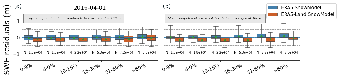
Figure A1 Distribution of the residuals between the SnowModel-simulated SWE and the ASO SWE at 100 m resolution in the Tuolumne River catchment (m w.e.) on 1 April 2016 (a) and 27 May 2016 (b), stratified by slope. Whiskers show the 5th to 95th percentiles, the line in each box represents the median of the distribution and the green triangle shows the mean. Slope has been calculated using the DEM at 3 m resolution and has been resampled with an average algorithm at 100 m.

Table A1 Correspondence table between Copernicus land cover and SnowModel vegetation classes. Correspondence table between Copernicus land cover and SnowModel (SM) vegetation classes.