Catchment landforms predict groundwater-dependent wetland sensitivity to recharge changes

This study investigates the influence of topography on the desaturation rates of groundwater-dependent wetlands in response to changes in recharge. We examined 60 catchments across northern Chile, which feature a wide variety of landforms. Landforms were categorized using geomorphon descriptors, resulting in three distinct clusters: flat, transitional, and mountain settings. Using steady-state three-dimensional (3D) groundwater models, we derived flow partitioning and seepage area extent for each catchment. Each cluster exhibited consistent seepage area evolution under varying wet to dry conditions. Our findings indicate that mountains have reduced seepage area compared to flats at equivalent hydraulic conductivity to recharge ($K/R$) ratios but are less sensitive to recharge fluctuations, with slower rates of seepage area reduction. Statistical analyses show that geomorphon-defined landforms correlate with desaturation indicators, enabling the prediction of catchment sensitivity to climate change based solely on topographic attributes.

1 Introduction

Changes in precipitation regimes and increasing temperatures driven by climate change are anticipated to significantly affect both surface and subsurface water resources (Berghuijs et al., 2024; Konapala et al., 2020; Taylor et al., 2013). Extended drought periods and reduced recharge are expected to threaten the functioning of groundwater-dependent ecosystems (Kløve et al., 2014; Rohde et al., 2024; Tetzlaff et al., 2024). These ecosystems rely on groundwater contributions to maintain their ecological structure and functional integrity, including processes that support biodiversity and key ecosystem services (Barron et al., 2014; Doody et al., 2017; Eamus and Froend, 2006). They encompass both terrestrial and aquatic environments, including wetlands, springs, rivers (riparian, aquatic, and hyporheic zones), lakes, grasslands, forests, and coastal and estuarine habitats (Eamus and Froend, 2006; Kløve et al., 2011). The extent to which groundwater-dependent ecosystems are vulnerable to climate-induced reductions in recharge depends not only on the hydrogeological properties of the underlying aquifer but also on the role of landscape morphology in shaping groundwater flow and discharge patterns (Gleeson and Manning, 2008; Singha and Navarre-Sitchler, 2022). Identifying the physical controls on groundwater emergence at the land surface is therefore essential to improve our ability to anticipate the responses of groundwater-dependent ecosystems to climate variability.

Groundwater seepage occurs when the water table intersects the topography. Thus, landforms influence both its spatial distribution and temporal dynamics (Bresciani et al., 2014, 2016; Sophocleous, 2002). The interaction between groundwater and topography significantly impacts the resilience of groundwater-dependent wetlands to climate variability (Cuthbert et al., 2019; Scanlon et al., 2023). Considering steady-state groundwater flow systems, the depth of the water table and the distribution of flow paths and groundwater seepage areas are controlled by the groundwater recharge rate (R), the topography, and the hydrodynamic properties of the aquifer through its hydraulic conductivity (K) (Condon and Maxwell, 2015; Rath et al., 2023; Tóth, 1963; Zhang et al., 2022). An equivalence of effects between R and K has been demonstrated (Bresciani et al., 2014; Haitjema and Mitchell-Bruker, 2005; Jamieson and Freeze, 1982), allowing a convenient focus on the dimensionless $\frac{K}{R}$ ratio and the topography. In non-anthropized contexts, the groundwater table is typically near the surface in low-relief and/or humid regions and deeper in rugged terrain and/or arid regions. However, the hydrogeological response and seepage dynamics to varying landscapes and topographic features are not straightforward and are difficult to predict.

Analytical solutions have been proposed to quantify the extent of groundwater seepage under varying $\frac{K}{R}$ at the hillslope scale, using simplified groundwater flow equations (Bresciani et al., 2014, 2016). Marçais et al. (2017) conducted modelling experiments to estimate seepage extent and dynamics using a two-dimensional (2D) representation of the equivalent hillslope. While these approaches are applicable in shallow aquifers, where flow predominantly follows the topography, they do not capture the complexity of three-dimensional (3D) groundwater flow, especially under low water tables or steep reliefs. A few 3D numerical modelling experiments have been undertaken, mainly for sensitivity studies with conceptual surface and subsurface geometries (Carlier et al., 2019; Gauvain et al., 2021; Gleeson and Manning, 2008; Welch et al., 2012). There is a pressing need to better understand the distribution and dynamics of groundwater seepage, particularly in light of the complex topographic characteristics of real-world landscapes and the 3D nature of groundwater flow. Such knowledge is critical for predicting the extent of seepage and the persistence of groundwater-dependent wetlands under future climate scenarios.

To address this knowledge gap, we designed a numerical experiment to model the partitioning of 3D groundwater flow and the extent of seepage across different landscapes, from flat to high mountain settings, under varying $\frac{K}{R}$ values. We applied this experiment on 60 catchments located in northern Chile, selected for their rich diversity of geomorphological contexts. By linking key topographic characteristics of the catchments to groundwater seepage dynamics predicted by the model, we aim to improve the prediction of wetland desaturation sensitivity under changing climate conditions. This approach supports the development of transferable frameworks for assessing the vulnerability of groundwater-dependent ecosystems across heterogeneous terrain and provides statistical means to regionalize our findings.

2 Material and methods

2.1 Geomorphological context

The study area is located in northern Chile between Santiago and the Peruvian border. The diversity of the landforms results from the specific tectonic and weathering processes involved in the Andes. This process resulted in the formation of a longitudinal valley called the Central Depression, which is bounded by two cordilleras, the Coastal Cordillera and the Principal Cordillera, both composed mainly of volcanic–sedimentary rocks (Hartley and Evenstar, 2010; Jordan et al., 1983). The Coastal Cordillera forms an intermediate mountain range with an average elevation between 1000–2000 m a.s.l., while the Principal Andean Cordillera has maximum elevations close to 7000 m a.s.l. (Fig. 1a) (Armijo et al., 2015; Charrier et al., 2007). The Central Depression delineates a sedimentary basin rich in Quaternary alluvial deposits with variable thicknesses, ranging from about 250 m near Santiago (Yáñez et al., 2015) to almost 1000 m in the northern regions of Chile (Hartley and Evenstar, 2010; Jordan et al., 2014; Nester and Jordan, 2011). Specifically, the Pre-Cordillera is a transition zone between the Central Depression and the Principal Cordillera, with catchment characteristics that vary from nearly flat terrain to mountainous regions with steep slope gradients and typical mountain front geomorphology (Fig. 1a). The diversity of these environments provides an excellent opportunity to explore a wide range of topographic settings, including flat catchments, mountain front areas, incised mountain catchments, volcanoes, and high mountain peaks.

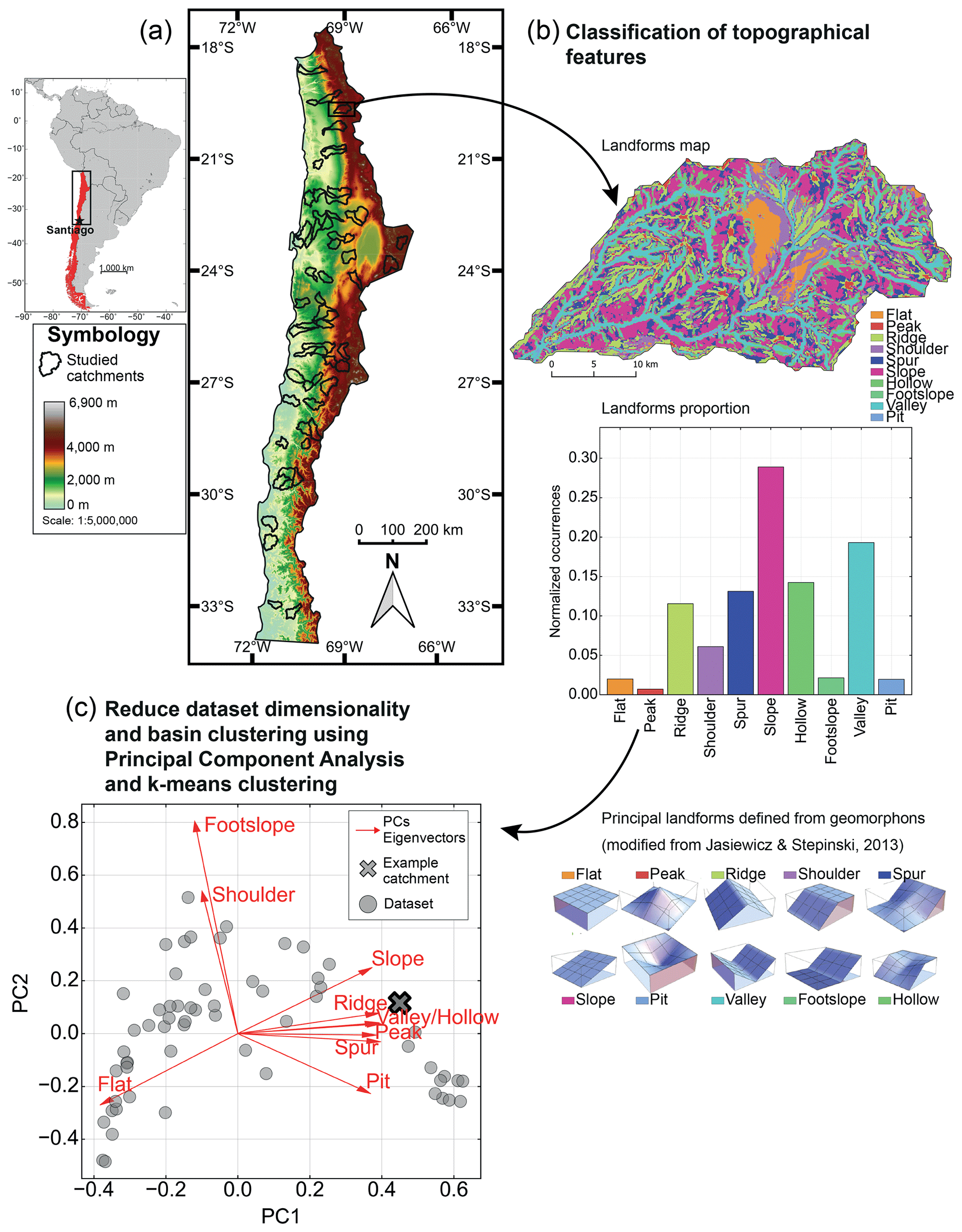
Figure 1 Methodological workflow for topographical classification and analysis. (a) Location and topographic map of the study area in northern Chile, with the boundaries of the 60 studied catchments highlighted in black. (b) Example of landform classification within a single catchment, including a landform map, the proportion of landform types, and an illustration of the principal landform categories defined by geomorphons (adapted from Jasiewicz and Stepinski, 2013). (c) Catchment categorization using principal component analysis (PCA) for dimensionality reduction and clustering. The example catchment is plotted in the PCA space, illustrating its position relative to the first two principal components (PC1 and PC2) and the whole dataset (grey dots). Red arrows represent the eigenvectors associated with different landform types, showing their contribution to the PCA axes.

2.2 Classification of catchment topographies

We considered the catchment boundaries of the global catchment database HydroATLAS (Lehner and Grill, 2013). We chose to limit the size of the catchments to between 500–1500 km² by considering level 8 of HydroATLAS. To cover different geomorphological and tectonic settings, we selected 60 catchments within our study area (indicated by black boundaries in Fig. 1a). We extracted the topography from the Shuttle Radar Topography Mission (SRTM; 90 m resolution) digital elevation model (DEM).

We used the geomorphon classification method proposed by Jasiewicz and Stepinski (2013) to categorize the landform features within each catchment, e.g. flat, peak, ridge, shoulder, spur, slope, pit, valley, footslope, and hollow. (Fig. 1b; note that geomorphon-defined landforms are italicized throughout the text for improved readability). This methodology is based on elevation differences in eight directions relative to the reference cell. This operation is reproduced for each cell of the DEM, identifying a shape for each of these cells (Fig. 1b). Unlike the direct cell neighbour method (e.g. slope, curvature, or roughness), the geomorphon method allows us to capture landforms at larger scales by defining a search radius around the reference cell, the look-up distance in Jasiewicz and Stepinski (2013). Here we defined the search radius equal to the hillslope characteristic length:

$$\begin{array}{}\text{(1)}& L={\displaystyle \frac{\mathrm{1}}{\mathrm{2}D}}\to L={\displaystyle \frac{\mathrm{1}}{\mathrm{2}\cdot \frac{l}{A}}},\end{array}$$

where L is the catchment feature length, l is the river network length, D is the drainage density, and A is the catchment area.

The river network is defined using a surface flow accumulation routine available in the Whitebox tool Python package (Lindsay, 2016). Combining principal component analysis (PCA) and k-means clustering methods (Fig. 1c), we categorized the catchments by their dominant landform features (Fig. 1b). PCA is a classical statistical method used to reduce the dataset dimensionality by transforming the original variables into a new set of uncorrelated variables, called principal components (PCs), which capture the maximum variance in the data. The k-means clustering approach allows us to identify groups of catchments belonging to the cluster with the nearest mean within the new PC space (Fig. 1c). Here, we defined three main clusters of catchments typical of flat, transitional, and mountain settings. Python code and trained models are available on the repository (Marti et al., 2025).

2.3 Numerical modelling of groundwater seepage extent

A three-dimensional numerical groundwater flow model was developed for each catchment. The models were constructed and run using the MODFLOW-2005 software suite (Harbaugh, 2005) with the NWT solver (Niswonger et al., 2011) and managed through the Python-based interface FLOPY (Bakker et al., 2016). The diffusivity equation was solved under steady-state conditions for unconfined flow.

The horizontal discretization followed the DEM resolution, set at 90 m (Fig. 2a), while the vertical discretization consisted of 10 layers with exponentially increasing thickness (Fig. 2b). To limit boundary effects, a buffer zone extending the model domain by 20 % around each catchment was added. A sensitivity analysis (Abhervé et al., 2023) of the extent of the buffer zone was performed to ensure that no impact on the seepage distribution was identified within the studied catchment (Fig. 2a). The model bottom mirrored the topography with a 100 m thick aquifer (Fig. 2b), assuming a constant aquifer thickness minimized the potential effects of transmissivity changes on seepage distribution. The 100 m thickness was chosen to realistically accommodate both flat sedimentary catchments and steep mountainous aquifers (Condon et al., 2020). The side and bottom boundaries of the buffer box were set as no-flow. For generality, effective recharge R was uniformly set at the water table across both the catchment and its buffer, enabling the simulation of both inflow and outflow across the model boundaries. This setup allowed us to consider interbasin groundwater exchanges, which are particularly likely to occur under low water table conditions (Fan, 2019). A drain boundary condition (with a conductance equal to the product of hydraulic conductivity with horizontal cell area divided by the cell mid-thickness) was set on the topography using the eponymous packages in MODFLOW to allow exfiltration of groundwater wherever the water table rose to intersect the land surface. This method ensures that discharge occurs naturally along the topography, mimicking surface-connected wetlands and springs without imposing fixed fluxes or predefined discharge zones.

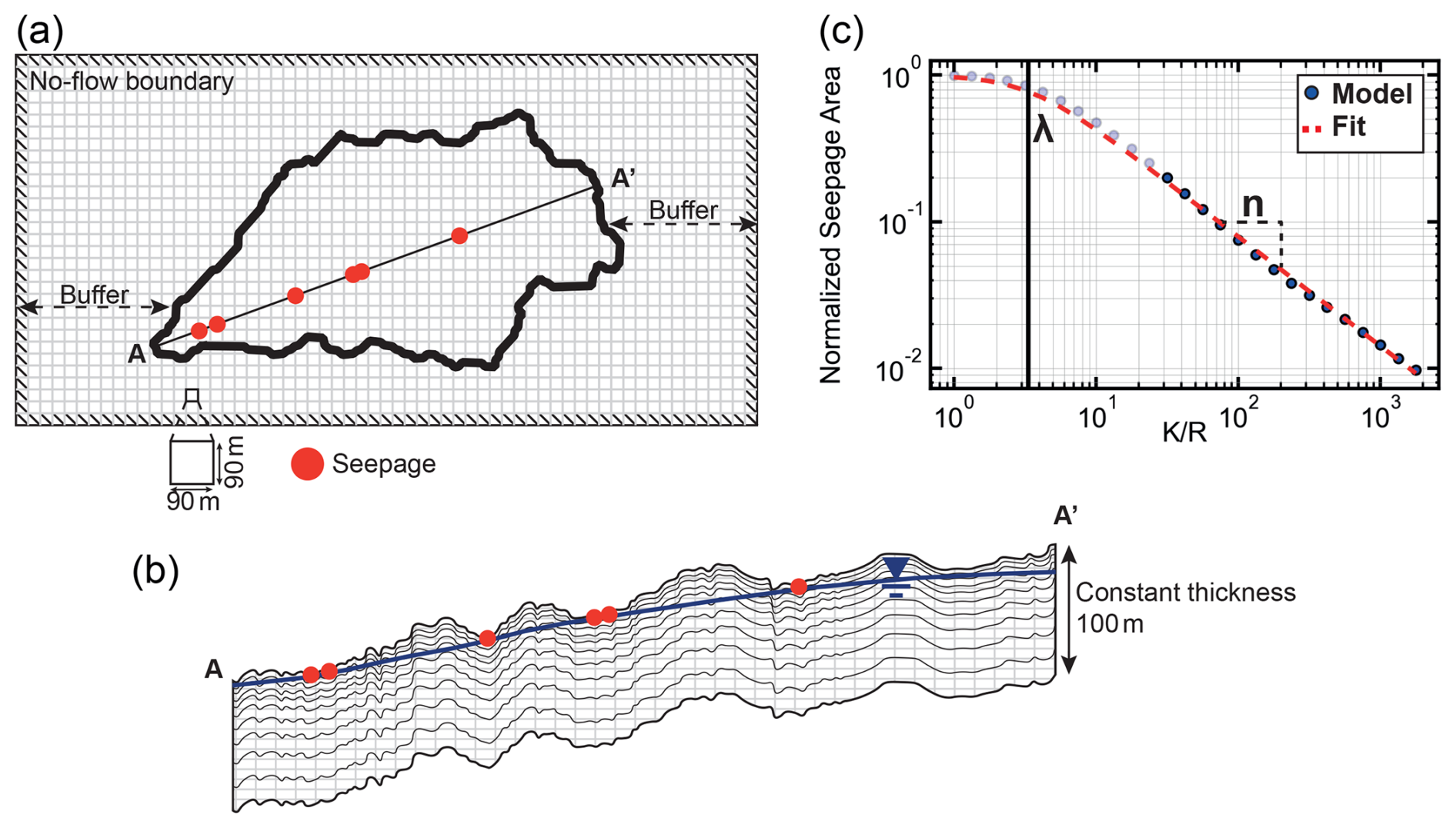
Figure 2 Model settings for one example catchment: (a) horizontal discretization and buffer zone beyond catchment limits, (b) AA' cross-section including vertical discretization and an arbitrary water table intercepting the topography creating seepage areas (red dots), (c) example of results of normalized seepage area with respect to $K/R$ (grey and blue dots) with the power law fit for Eq. (2a) (dashed red curve). The blue dots represent the normalized seepage area <20 % where the fit weight is enhanced.

To solely focus on the effects of topography in the redistribution of groundwater seepage, we imposed homogeneous and isotropic hydraulic conductivity (K) across all modelled catchments. This simplification ensures that variability in seepage behaviour arises solely from differences in landscape geometry and water table positions, rather than site-specific geological heterogeneity. Various water table positions relative to the topography were derived by setting different values of the $\frac{K}{R}$ ratio, ranging from 100 for fully saturated conditions to 10 000 when all simulated catchments were nearly fully desaturated (i.e. when the normalized seepage area $S_{\mathrm{A}}^{\ast }=\frac{\text{seepage area}}{\text{catchment area}}$ reaches 1 %). $\frac{K}{R}$ values were logarithmically spaced within this interval, and simulations were stopped if the catchment's seepage area fell below the 1 % threshold (Fig. 2c). This allows us to consider a full range of conditions from humid to arid climates and low to high hydraulic conductivity settings. This modelling workflow resulted in a total of 1793 simulations.

For each catchment, we perform a power law fit on the relationship between seepage area extent and $\frac{K}{R}$, further mentioned as the desaturation function (Eq. 2a and red curve in Fig. 2c). This allows us to capitalize on the observed linear relation between $\log (S_{\mathrm{A}}^{\ast }$) and $\log (\frac{K}{R}$):

$$\begin{array}{}\text{(2a)}& {\displaystyle }& {\displaystyle }{S}_{\mathrm{A}}^{\ast }={\left(\mathrm{1}+{\left({\displaystyle \frac{\frac{K}{R}}{\mathit{\lambda }}}\right)}^{\mathrm{2}}\right)}^n\text{(2b)}& {\displaystyle }& {\displaystyle \frac{\text{d}{S}_{\mathrm{A}}^{\ast }}{\text{d}\frac{K}{R}}}={\displaystyle \frac{\mathrm{2}n}{{\mathit{\lambda }}^{\mathrm{2}}}}{\displaystyle \frac{K}{R}}{\displaystyle \frac{S_{\mathrm{A}}^{\ast }}{\mathrm{1}+{\left(\frac{\frac{K}{R}}{\mathit{\lambda }}\right)}^{\mathrm{2}}}}\text{(2c)}& {\displaystyle }& {\displaystyle \frac{\text{d}{S}_{\mathrm{A}}^{\ast }}{\text{d}\frac{K}{R}}}\approx {\displaystyle \frac{\mathrm{2}n{S}_{\mathrm{A}}^{\ast }}{\frac{K}{R}}}\text{when }{\displaystyle \frac{K}{R}}\gg \mathit{\lambda }.\end{array}$$

The desaturation function is determined by the proportionality constant, λ, which can be associated with a desaturation threshold, i.e. the critical value of $\frac{K}{R}$ above which the catchment begins to desaturate. The negative desaturation exponent, n, directly affects the rate of change in seepage extent as $\frac{K}{R}$ increases, as shown in Eqs. (2b) and (2c). It can be viewed as a measure of the sensitivity of the seepage area extent to a deepening of the water table: for a given pair of seepage area and $\frac{K}{R}$, a lower n indicates a higher sensitivity of the catchment to a decrease in the water level. We estimated n considering seepage area extents lower than 20 % of the catchment area, which are more representative of real-world conditions, i.e. by giving more weight in the fit to the higher $\frac{K}{R}$ ratios.

2.4 Regionalization with random forest algorithm

To predict the desaturation response metrics λ and n from topographic descriptors and regionalize our findings, we employed random forest regression using the scikit-learn library in Python (Pedregosa et al., 2011). The input features for the model were the first two principal components (PC1 and PC2) derived from the 60 catchments. Random forest models were trained independently for λ and n. Model performance and robustness were assessed using a bootstrap resampling procedure with 5000 iterations. In each iteration, 10 catchments were randomly selected as a test set, while the remaining 50 were used for training. The coefficient of determination (R²) was calculated on the test data for each iteration, and the resulting R² distribution was used to evaluate model reliability (see Sect. S2 for the kernel density estimate of R² values). Hyperparameter tuning for each model was performed using GridSearchCV with 2-fold cross-validation within each training subset. The tested parameter grid included $\text{n\_estimators}\in \mathit{\{}\mathrm{50},\mathrm{200},\mathrm{500},\mathrm{1000}\mathit{\}}$ and $\text{max\_depth}\in \mathit{\{}\text{none},\mathrm{2},\mathrm{10},\mathrm{20}\mathit{\}}$. The best combination of hyperparameters was used to retrain the model on the full training set in each iteration. The final random forest model was defined as the one achieving the best trade-off in predictive accuracy for both λ and n, and it was applied to predict desaturation metrics in 63 additional catchments located in southern Chile.

3 Results

3.1 Typology of catchment topography

We evaluate the proportion of main geomorphons on the 60-catchment dataset. The PCA (Fig. 1c) resulted in a first component (PC1) explaining 75.4 % of the total variance and in the first two components (PC1 and PC2) combined explaining 86.8 % of the total variance. This result indicates a strong relation between the landform description from geomorphon analysis in the catchments and the reduction into two dimensions. We found that PC1 mostly represents the differentiation between flat and slope landforms, with eigenvector magnitudes of −0.4 for the flat landform and 0.4 for the slope landform. Slope landform is associated with the peak, ridge, valley, hollow, spur, and pit forms, all showing similar eigenvector magnitudes on PC1. Regarding PC2, the footslope and shoulder forms are the main control, with eigenvector magnitudes of 0.8 and 0.5, respectively. Flat and slope forms show eigenvector magnitudes of −0.2 and 0.2 along the PC2 axis.

To further support and illustrate this description, the catchments are grouped into three clusters, as a result of the k-means clustering, displayed with different colours in Figs. 3 and 4. The red cluster is characterized by relatively flat landforms. Conversely, the blue cluster is strongly influenced by slope and associated landforms along PC1 (ridge, valley, peak) representative of mountain catchments with incised valleys and narrow valley bottoms. The green cluster exhibits more dispersion in the represented catchments. This cluster acts as a transition between the red and blue clusters. It contains catchments most influenced by footslope and shoulder forms. Positioned centrally between the two extreme clusters, this cluster serves as a transition zone between flatter areas and mountain catchments, possibly including catchments showing both flat and mountainous characteristics, as observed at mountain fronts.

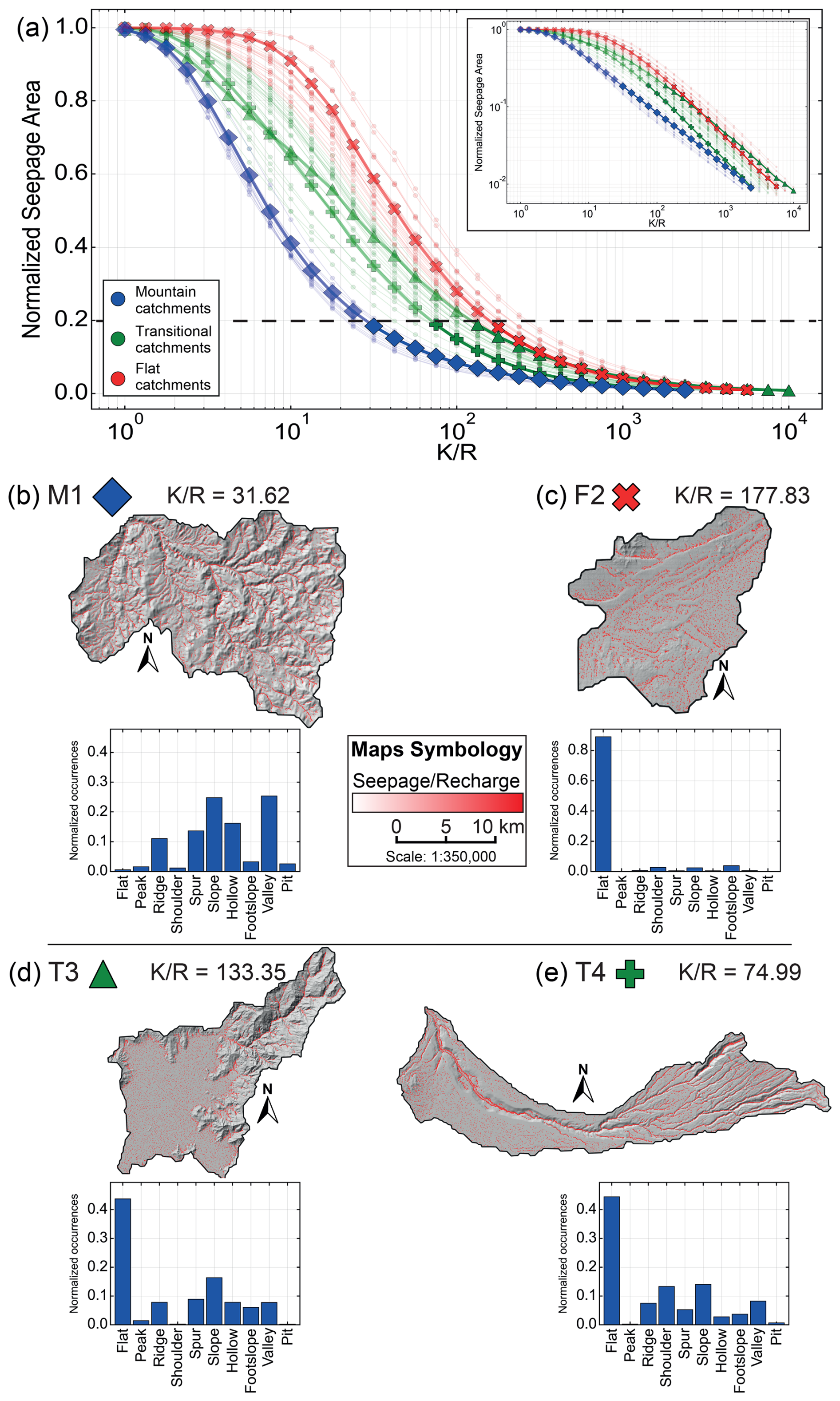
Figure 3 (a) Normalized seepage area against $\frac{K}{R}$ for the 60 catchments (coloured lines with markers), including a log–log plot in the upper-right corner. Four illustrative catchments are highlighted: mountain type M1 (blue diamond, b), flat type F2 (red cross, c), transitional type T3 (green triangle, d), and T4 (green cross, e). Details include the topographic map overlaid by the seepage extent at an arbitrary value of 20 % (red mask), with the corresponding $\frac{K}{R}$ value along with the landform distribution statistics.

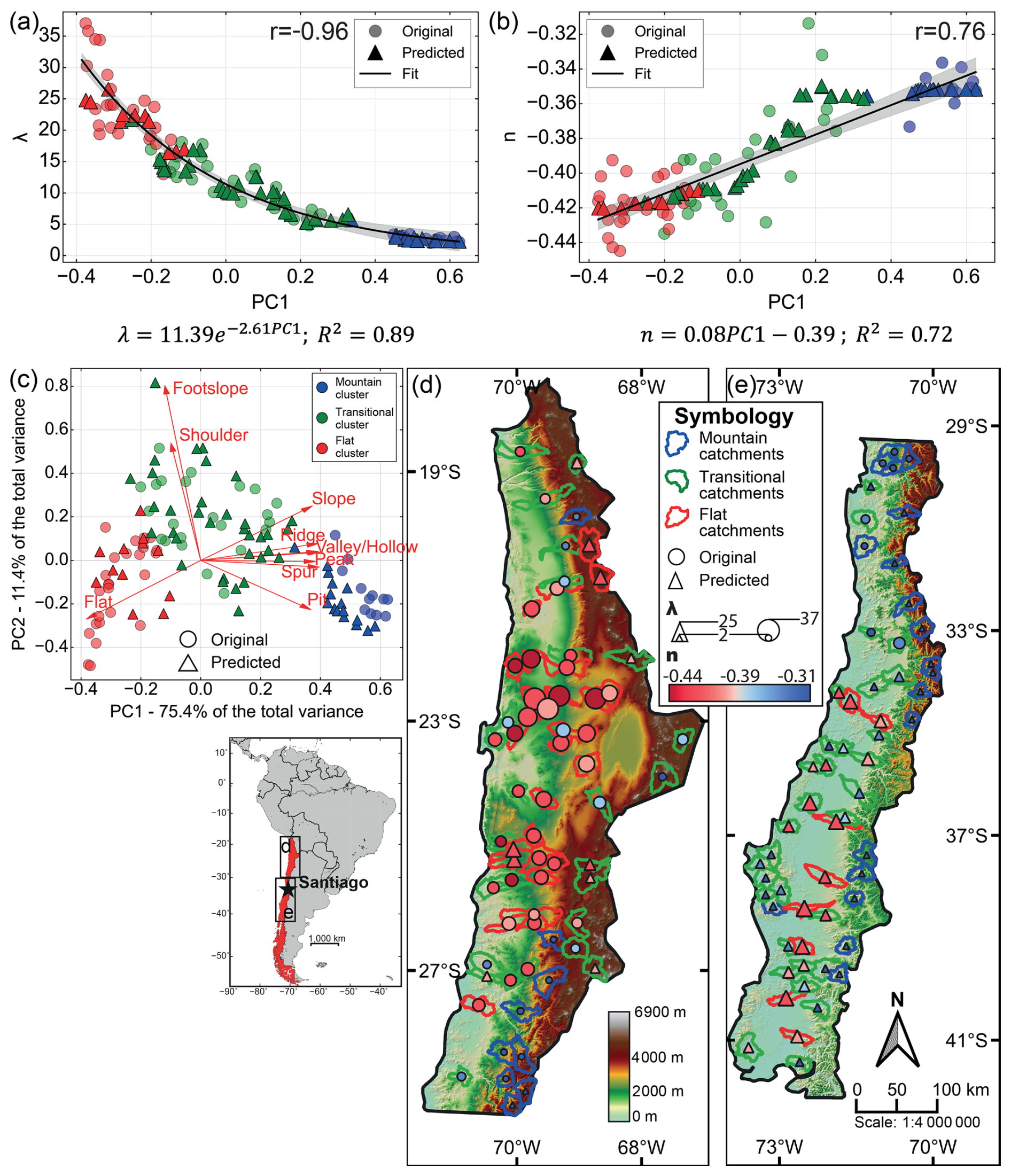
Figure 4 Scatter plots for the original 60-catchment dataset (dots) with the Spearman coefficient r, the equation, and the coefficient of determination (R²) of a global fit (black line with 95 % confidence interval) for (a) λ against PC1 and for (b) n against PC1. Random forest predictions for both parameters are superimposed on the original data (triangles). (c) PCA plot for the original (dots) and prediction (triangles) datasets. The percentage of variance in the original dataset explained by each component is displayed in the axis title. (d, e) Situation and topographic maps of the study area highlighting the 123 catchments with different colours according to the defined catchment clusters (flat, transitional, and mountain). Each catchment is marked by a dot (original dataset) or a triangle (prediction dataset) whose size depends on λ and whose colour depends on n.

To facilitate comprehension and illustration, the catchment clusters are referred to as flat catchment for the red cluster, mountain catchment for the blue cluster, and transitional catchment for the green cluster hereafter.

3.2 Seepage distribution evolution with increasing $\frac{K}{R}$

Figure 3a illustrates the evolution of seepage area, normalized by catchment area, as a function of $\frac{K}{R}$ for all 60 catchments. Four specific catchments are highlighted with sharper lines for further discussion. As expected, lower $\frac{K}{R}$ values result in fully saturated catchments, while, as $\frac{K}{R}$ increases, all catchments progressively desaturate at varying rates. For instance, at a normalized seepage area of 20 %, the corresponding $\frac{K}{R}$ values range from 20 to 250.

The desaturation behaviour can be clearly differentiated for the three clusters of catchments (Fig. 3a), confirming that variations in seepage distribution are predominantly driven by topographical effects. The power law fit of seepage distribution (Eq. 2a) for each of the 60 catchments results in λ values ranging from 2.05 to 37.03 and n values ranging from −0.44 to −0.31. The fit shows minimal RMSE values between 0.01 and 0.08, indicating that seepage evolution with increasing $\frac{K}{R}$ can be successfully parameterized with only two parameters, λ and n.

Regarding the desaturation threshold, λ, the mountain catchments show lower values than the flat ones. The transitional catchments show intermediate behaviour, reaching higher λ values than the mountain catchments but lower λ values than the flat ones. Regarding the desaturation exponent, n, within the low-saturation domain (≤20 %), the mountain catchments exhibit slower desaturation rates, while the flats present faster desaturation rates. The variability in desaturation slopes for the transitional catchments is more pronounced, reflecting a mix of behaviours within this zone, yet it again shows intermediate behaviour relative to the other two clusters.

3.3 Groundwater seepage extent in four representative catchments

Figure 3 highlights four distinct catchments: M1, representative of the mountain catchments; F2, representing the flat catchments; and T3 and T4, showing the range of responses within the transitional catchments. We present the seepage over recharge distribution overlaid on the topographic map and the landform proportions for each catchment (Fig. 3b–e).

For M1 (Fig. 3b), characterized by low λ and high n values, it exhibits the typical seepage distribution of mountainous regions. At a normalized area of 0.2, seepage primarily congregates in topographic lows, such as river valleys, while ridges and peaks desaturate due to their significant elevation compared to the surrounding terrain. Conversely, F2 (Fig. 3c), with high λ and low n values, suggests that the water table remains closer to the surface in flat settings. For T3 and T4, their landform proportions (Fig. 3d and e) reveal similar values for most forms, except for a higher proportion of shoulder and footslope forms in T4. This increased prevalence of shoulder landform in T4 is due to a prominent incised river valley in the eastern part of the catchment.

Examining T3's seepage distribution, it initially aligns with the mountain catchments with a low desaturation threshold (λ). Then, in the range of $\mathrm{1}<\frac{K}{R}<\mathrm{10}$, a substantial change in the desaturation function is observed, with the distribution pattern converging toward the ones typical of the flat catchments for high $\frac{K}{R}$ values, ultimately being the last catchment to reach a saturation level of <1 %. This behaviour can be explained by looking at the spatial distribution of seepage for T3 (Fig. 3d). A clear contrast exists between the flat western area and the mountainous settings to the east. At higher elevations, desaturation occurs at lower $\frac{K}{R}$ values dominated by the steep landforms of the mountain settings and resulting in a low desaturation threshold (λ). Subsequently, at a normalized area of 0.2, the catchment desaturation is mostly controlled by the western flat terrains.

Conversely, T4's seepage distribution exhibits the opposite pattern. It initially mirrors the flat cluster with a higher λ value, ultimately resembling the mountain cluster characteristics, reaching saturation levels under 1 % for similar $\frac{K}{R}$ values. The seepage spatial distribution for T4 (Fig. 3e) shows that flat landforms at higher-elevation zones in the western part of the catchment control the initiation of the desaturation before being mostly controlled by the steep incised valley at lower elevations, which tends to sustain the seepage extent.

3.4 Linking topographic features and desaturation behaviour

We computed the correlation matrix between the principal components (PC1 and PC2) and the desaturation parameters (λ and n) to assess the strength of the topographical control on desaturation behaviour. Figure 4a shows a strong anti-correlation between λ and PC1, with a Spearman coefficient of $r=-\mathrm{0.96}$ (p<0.0001). Figure 4b displays a strong linear correlation between n and PC1, with r=0.76 (p<0.0001). No other significant correlations were identified (the entire correlation matrix is available in Sect. S1 in the Supplement).

The catchment clusters are well distinguishable in Fig. 4a and b. In Fig. 4a, the inverse relationship between λ and PC1 is robustly quantified by fitting an exponential function (R²=0.89), facilitating a quantitative correlation between λ and PC1, as illustrated in Fig. 4a. The mountain cluster is isolated with a low average and variance in λ values. The transitional cluster forms the elbow part of the exponential decay, while the flat cluster is clearly identified with higher λ values. The variations in λ values are higher in the flat and transitional catchments compared to the mountain ones.

Figure 4b reveals a linear relationship between n and PC1. The good linear fit (R²=0.72) allows a straightforward quantification of the relationship between PC1 and the negative scaling exponent n and, consequently, the appraisal of the desaturation rate based on landforms (Eqs. 2b and c). The catchment clusters are well identified, with the flat cluster showing lower n values than the mountain cluster.

We finally employed a random forest regression on the dataset to predict λ and n based on topographic parameters (PC1 and PC2) for 63 catchments located both in the same study area and expanding further south inside Chile (Fig. 4d and e). We defined PC1, PC2, and clusters for these new catchments using the originally trained PCA and k-means models (Fig. 4c). Predictions made for λ (Fig. 4a) show good consistency with the original dataset both in terms of identifying clusters behaviours and in trend, following the originally defined exponential relation. Regarding n (Fig. 4b), we observe a similar accuracy to represent clusters, while the general linear trend is less obvious. We observe for n, while following an increasing trend, a diversified response between the clusters, with the transitional catchments exhibiting a greater rate of change in n for an equivalent increment in PC1. However, the spatial distribution of the predicted catchments observed in Fig. 4d and e is a good match with the original data, in terms of both topographic characteristics and desaturation function parameters.

4 Discussion and perspectives

Groundwater flow and storage regulate the resilience of wetlands to climate variability (Fan et al., 2019). Variations in topography and landforms across catchments lead to differences in wetland sensitivity to changing recharge by shaping distinct groundwater flow structures. In this study, we provide a quantitative assessment of the controls of landforms on the sensitivity of groundwater-dependent wetlands to aquifer desaturation – expressed through variations in the $\frac{K}{R}$ ratio – across a total of 123 catchments in Chile, spanning settings from flat to high mountain topographies. These feedback mechanisms were analysed using a novel combination of three-dimensional process-based groundwater modelling, geomorphon-based landform classification, multivariate statistical analysis, and random forest predictions at the regional scale.

Moreover, the proposed methodology demonstrated strong robustness to outliers and atypical landscape configurations. For instance, the Andes Mountains in northern Chile encompass the “Altiplano” region, which features extensive flat terrains within an otherwise mountainous setting. The method successfully identified such catchments and classified them as flat (Fig. 4d between 19 and 23° S), illustrating its ability to reliably capture dominant landform characteristics across diverse geomorphological contexts.

Our results demonstrate that the desaturation functions of catchments can be explained by the typologies in topography derived from landform categorization. Building on previous works that focused on two-dimensional aquifer geometry, as first introduced by Haitjema and Mitchell-Bruker (2005) and further explored by Bresciani et al. (2014), we show that mountainous regions exhibit lower seepage extents, restricted to incised valleys, compared to flat catchments at equivalent $\frac{K}{R}$ ratios. However, we demonstrate that mountainous regions are less sensitive to changes in saturation, exhibiting slower desaturation rates.

To disentangle the respective impacts of different landforms, we compared our results with those obtained from the analytical solution proposed by Bresciani et al. (2014) for a 1D hillslope, where one can easily assess the impacts of slope angle and the concavity/convexity of the hillslope (results in Sect. S3). In agreement with our results, the steepness of the hillslope is the primary influence on seepage extent and its variation through changes in groundwater level. Steep slopes begin to desaturate at lower $\frac{K}{R}$ values than gentler slopes. Additionally, for a given change in groundwater level, the rate of change in seepage extent is inversely correlated with slope angle. This aligns with the differences in the desaturation exponent, n, and the desaturation threshold, λ, obtained for the mountain and flat clusters. Mountain clusters have higher n and lower λ values, suggesting higher resilience to changes in $\frac{K}{R}$.

Furthermore, the analysis of the simple analytical solution demonstrates that hillslope shape (concave vs. convex) also affects the desaturation function, though to a lesser extent than slope. Concave slopes appear to have a lower λ but a higher n than convex slopes. Similarities between concave and convex hillslopes can be found in the shoulder vs. footslope in our landform classification. Shoulder and footslope are differentiated primarily along PC2, explaining a smaller proportion of the variance in the dataset analysed here. However, no clear correlation between PC2, n, and λ was found, suggesting a minimal impact of shoulder and footslope landforms compared to the other ones.

While the aim of the present work is to establish a comprehensive exploration of landform controls on seepage dynamics, several simplifications limit its direct application to specific real-catchment systems. Although the models are based on real topographies from the Chilean Andes, the experiment does not intend to capture actual complexity of hydrogeological systems but rather to explore a wide enough range of natural landform geometries for comparative analysis. Firstly, we assumed homogeneous and isotropic aquifer properties with a fixed aquifer thickness, thereby neglecting geological heterogeneities, anisotropy, and variability in the depth of the active groundwater flow system (Frisbee et al., 2017; McIntosh and Ferguson, 2021), and consequently the seepage distribution, that can be involved in real landscape. While our use of the dimensionless $\frac{K}{R}$ ratio offers a robust approach for analysing desaturation responses, future research could benefit from exploring additional parameters that account for catchment geometry, relief, or flow system depth. Additionally, the model results presented here operate under steady-state conditions and exclude the potential impacts of seasonal recharge variability, vegetation feedbacks, or the role of the unsaturated zone near the land surface. Exploring such processes, especially under transient conditions and with heterogeneous parameters, represents a promising perspective for future research.

5 Conclusions

To conclude, our study demonstrates that catchment-scale topographic features, quantified through geomorphon-based landform classification, exert a first-order control on groundwater seepage dynamics under varying recharge conditions. By linking these landforms to a desaturation function, we show that the sensitivity of groundwater seepage extent to climate variability can be predicted from topography alone. This insight enables the development of a robust and scalable framework for assessing hydroclimatic vulnerability, particularly relevant for data-scarce regions. The ability to regionalize desaturation behaviour using simple statistical learning tools, such as random forest as presented here, opens up new opportunities for applying this approach to ungauged basins in other regions (Hrachowitz et al., 2013). As such, our findings not only offer a methodological advance but also demonstrate the potential to assess the vulnerability of groundwater-dependent wetlands and the ecosystem they support to climate change.