The value of observed reservoir storage anomalies for improving the simulation of reservoir dynamics in large-scale hydrological models

Human-managed reservoirs alter water flows and storage, impacting the hydrological cycle. Modeling reservoir outflow and storage, which affect water availability for humans and freshwater ecosystems, is challenging because they depend on human decisions. In addition, access to data on reservoir inflows, outflows, storage, and operational rules is very limited. Consequently, large-scale hydrological models either exclude reservoir operations or use calibration-free algorithms to model reservoir dynamics. Nowadays, estimates of reservoir storage anomalies based on remote sensing are a potential resource for calibrating the release algorithms for many reservoirs worldwide. However, the impact of calibration against the storage anomaly on simulated reservoir outflow and absolute storage is unclear. In this study, we address this by using in situ outflow and storage data from 100 reservoirs in the USA (ResOpsUS dataset) to calibrate three reservoir operation algorithms: the well-established Hanasaki algorithm (CH) and two new storage-based algorithms, the Scaling algorithm (SA) and the Weighting algorithm (WA). These algorithms were implemented in the global hydrological model WaterGAP, with their parameters estimated individually for each reservoir and four alternative calibration targets: monthly time series of (1) the storage anomaly, (2) estimated storage (calculated based on the storage anomaly and GRanD reservoir capacity), (3) storage, and (4) outflow. The first two variables can be obtained from freely available global datasets, while the latter two variables are not publicly accessible for most reservoirs. We found that calibrating against outflow did not result in skillful storage simulations for most of the 100 reservoirs and only slightly improved outflow simulations compared to calibration against the three storage-related targets. Compared to the non-calibrated Hanasaki algorithm (DH), calibrating against both the storage anomaly and estimated storage improved the storage simulation, whereas the outflow simulation was only slightly improved. Calibration against the storage anomaly yielded skillful storage simulations for 64 (39), 68 (45), and 66 (45) reservoirs in the case of CH, SA, and WA, respectively, during the calibration (validation) period, compared to just 16 (15) for DH. Using estimated storage instead of the storage anomaly does not offer any added benefit, primarily due to inconsistencies in the observed maximum water storage and storage capacity data from GRanD. The default parameters of the Hanasaki algorithm rarely matched the calibrated parameters, highlighting the importance of calibration. Using observed inflow rather than simulated inflow has a greater impact on improving the outflow simulation than calibration, whereas the opposite is true for the storage simulation. Overall, the performance of the SA and WA algorithms is nearly equal, and both outperform the CH and DH algorithms. Moreover, incorporating downstream water demand into the reservoir algorithms does not necessarily improve modeling performance due to the high uncertainty in demand estimation. Therefore, to improve the modeling of reservoir storage and outflow in large-scale hydrological models, we recommend calibrating either the SA or the WA reservoir algorithm individually for each reservoir against the remote-sensing-based storage anomaly, unless in situ storage data are available, and improving the reservoir inflow simulation.

1 Introduction

Globally, over 58 000 large dams (at least 15 m high) capable of impounding 8300 km³ have been constructed to meet various human needs, including irrigation, flood control, hydropower generation, domestic water supply, and recreation (Chao et al., 2008; Perera et al., 2021). These dams store approximately one-sixth of the annual streamflow in reservoirs (Hanasaki et al., 2006), significantly altering the global freshwater system by increasing evaporation and modifying downstream streamflow (Best, 2019; Tian et al., 2022). About 60 % of the seasonal variability in Earth's surface water storage is attributed to human-managed reservoirs, i.e., artificial reservoirs and regulated lakes, since the water level of these reservoirs varies on average 4 times more than that of natural lakes (Cooley et al., 2021). Therefore, to accurately depict the hydrologic cycle and assess the impact of reservoir operations on water availability for humans and freshwater ecosystems, including the dynamics of human-managed reservoirs in hydrological models is crucial. Currently, 6 out of the 16 global hydrological models contributing to ISIMIP2 (The Inter-Sectoral Impact Model Intercomparison Project, http://www.isimip.org, last access: 28 August 2025) simulate the dynamics of human-managed reservoirs (Telteu et al., 2021).

Whereas the outflow from a natural lake strongly depends on the lake's water level and thus the water storage in the lake, humans manage the outflow from a reservoir. Although human decisions regarding the release of water from reservoirs depend, to some extent, on the reservoir's water storage, they are also affected by various other factors, such as downstream water demand, the need for hydropower production, flood protection for downstream areas, ecosystem needs, and legal constraints (Jager and Smith, 2008; Dong et al., 2023). Most reservoirs serve multiple purposes, making their simulation even more complex. However, because the operational (i.e., release) rules of reservoirs and observed data on reservoir inflow, outflow, and storage dynamics are rarely publicly available, large-scale hydrological models must resort to calibration-free reservoir operation algorithms that only require information about the reservoir's storage capacity and surface water area. These algorithms are considered calibration-free because they do not require the calibration of reservoir-specific parameters based on observations of model output variables. While these algorithms can simulate the decisions of reservoir operators to some extent, they do not account for the unique operational patterns of each reservoir (Masaki et al., 2018; Turner et al., 2021; Steyaert and Condon, 2024).

All global hydrological models currently employ calibration-free reservoir operation algorithms, which vary in their formulation and complexity (Telteu et al., 2021). Examples of calibration-free reservoir operation algorithms proposed for large-scale hydrological modeling are described in Dong et al. (2022), Zajac et al. (2017), Haddeland et al. (2006), and Hanasaki et al. (2006) (herein referred to as H06). Dong et al. (2022) and Zajac et al. (2017) employed different operational rules for four distinct levels of reservoir storage in their algorithms, whereas Haddeland et al. (2006) developed a prospective optimization algorithm tailored to the reservoir's purpose. The H06 method is currently implemented in the global hydrological model H08 (Hanasaki et al., 2008) and, in a slightly modified form, in the global hydrological model WaterGAP. It also serves as the basis for the Dam-Reservoir Operation model (DROP; Sadki et al., 2023). While studies (e.g., Döll et al., 2009; Vanderkelen et al., 2022) clearly demonstrate that implementing the H06 algorithm leads to improved streamflow simulations compared to completely disregarding the reservoir as a surface water body, there is no consensus (please refer to Döll et al., 2009; Vanderkelen et al., 2022; Gutenson et al., 2020) on whether the H06 algorithm outperforms the natural lake outflow parameterization of Döll et al. (2003) (herein referred to as D03), which assumes that artificial reservoirs behave similarly to natural lakes. It should be noted that the simulated reservoir outflow and storage dynamics depend not only on the reservoir operation algorithm but also on the quality of the simulated inflow, making it challenging to assess the adequacy of the algorithm without inflow observations (Vanderkelen et al., 2022).

Several studies have endeavored to fine-tune calibration-free algorithms by adjusting a single parameter for each reservoir, but the results have been unpromising. For example, Gutenson et al. (2020) found that adjusting only one parameter of H06 for 60 non-irrigation reservoirs across the US did not lead to better simulations compared to a calibrated D03. Shin et al. (2019) reported that a new algorithm based on H06, with one parameter calibrated for 27 reservoirs, could not accurately capture the seasonality in reservoir storage and outflow. As a result, some studies have devised calibration-required algorithms with multiple parameters for each reservoir. Turner et al. (2021) introduced the Inferred Storage Targets and Release Functions (ISTARF) approach, a reservoir operating policy comprising 19 parameters. This approach was applied to 1930 reservoirs across the US and demonstrated robust improvements in both outflow and storage compared to the H06 model. Although the ISTARF approach is relatively parsimonious in terms of the number of parameters compared to other established calibration-required algorithms – such as those proposed by Yassin et al. (2019) and Turner et al. (2020), which feature 72 (six parameters for each month) and 208 parameters per reservoir (four parameters for each week), respectively – integrating these approaches into large-scale models incurs substantial computational costs. More importantly, this approach requires time series data of observed inflow, outflow, and reservoir storage, which can be difficult to obtain outside the US, rendering them unfeasible for global-scale modeling. The same limitation applies to some machine learning approaches for simulating reservoir dynamics, such as the artificial neural network approach proposed by Ehsani et al. (2016) and the tree-based reservoir model developed by Chen et al. (2022).

Remotely sensed data on water levels and surface water area of reservoirs are increasingly available. They are being used to derive time series of water storage anomalies or even absolute storage. With recent advancements in spaceborne data, such as the Surface Water and Ocean Topography (SWOT) mission, storage anomaly data can now be gathered even for small reservoirs, providing a valuable source for enhancing reservoir modeling within large-scale hydrological models (Biancamaria et al., 2016). Examples include HydroSat (Tourian et al., 2022), the Global Reservoir Storage (GRS) dataset (Li et al., 2023), and GloLakes (Hou et al., 2024). This newly available information could be used to calibrate reservoir operation algorithms individually for each reservoir, which is expected to lead to an improved simulation of reservoir dynamics. Remote-sensing-derived reservoir storage anomalies were shown to fit reasonably well with in situ observations, depending on the reservoir and satellite data product. Storage anomalies, rather than absolute water storage values, should be considered for both simulated and remote sensing data (Otta et al., 2023). In this regard, Hanazaki et al. (2022) developed a targeted storage-and-release algorithm for global flood modeling, where the release is estimated for four storage zones based on the volume of each zone, flood discharge, and long-term average inflow. They estimated the volume of each storage zone using remote sensing data, while calculating flood discharge with a probability distribution for 2169 dams worldwide. The authors reported a 62 % improvement in Nash–Sutcliffe efficiency compared to the version of the CaMa-Flood global hydrodynamic model that did not include the reservoir module. Recently, supported by remote sensing data and a machine learning approach, Shen et al. (2025) developed a satellite-based target storage reservoir operation scheme (SBTS) with seven parameters. This scheme simulates the outflow and storage of flood control reservoirs across four distinct storage zones, utilizing estimated flood storage capacity (FSC) data for 1178 reservoirs, derived from machine learning trained on reported FSC data from 436 reservoirs. They found that their approach, when using observed inflow, improves reservoir parameterizations, enabling the SBTS to generally outperform the methods of Dong et al. (2022), Zajac et al. (2017), and Hanazaki et al. (2022). However, they reported no improvement when the simulated inflow was used. Dong et al. (2023) demonstrated that simultaneous calibrations against reconstructed release and reservoir storage data (using remotely sensed data, model simulations, and in situ data) considerably improved the performance of reservoir operation algorithms for the Ertan and Jinping I reservoirs in China. However, for global-scale studies, release information is unavailable for most reservoirs. In such cases, calibrating against the storage anomaly alone for parameter estimation may degrade outflow simulations due to potential trade-offs between calibrating against different variables (Döll et al., 2024; Hasan et al., 2025). The recently published dataset of observed dynamics of US reservoirs, “ResOpsUS” (Steyaert et al., 2022), which provides time series of daily observed storage, elevation, inflows, and outflows for up to 679 reservoirs across the contiguous US, offers an opportunity to explore this trade-off.

The primary objective of this study is to investigate how monthly time series of observed reservoir-related data can improve the simulation of reservoir outflow and storage in continental or global hydrological models. We focus on the suitability of observed storage anomalies for calibrating reservoir operation algorithms, as these anomalies can be obtained globally through remote-sensing-based observations. We compare their informational value to that of scarcer outflow and absolute storage observations, along with the simulation results obtained from an uncalibrated reservoir algorithm. We utilized in situ storage and outflow data from the ResOpsUS dataset for 100 reservoirs in the US to calibrate three reservoir operation algorithms. All algorithms were implemented in the global hydrological model WaterGAP 2.2e (Müller Schmied et al., 2024). The parameters of the algorithms were estimated using the following alternative calibration targets: (1) the storage anomaly, (2) estimated storage (calculated based on the storage anomaly and GRanD reservoir capacity, detailed in Sect. 2.3), (3) storage, and (4) reservoir outflow. Calibration involved optimizing parameters individually for each reservoir, algorithm, and calibration target. Additionally, to explore the sensitivity of the model results to the quality of the inflow data, we calibrated the algorithms for a subset of 35 reservoirs with available inflow measurements, using observed inflow instead of the inflow simulated by WaterGAP. Finally, for a subset of 21 reservoirs, we evaluated the impact of including downstream water demand in the algorithms for irrigation and water supply reservoirs.

2 Methods and data

2.1 The global hydrological model WaterGAP

WaterGAP simulates the dynamics of water flows and storage on the continents as impacted by human water use and human-managed reservoirs (Müller Schmied et al., 2021). It calculates sectoral water abstractions, along with net abstractions (abstraction minus return flows), from surface water bodies (such as reservoirs, lakes, and rivers) and groundwater. The model has a spatial resolution of 0.5° × 0.5° and a daily temporal resolution. However, model output analysis is typically conducted on a monthly scale. The current version, 2.2e, has been calibrated in a basin-specific manner against the mean annual streamflow at 1509 gauging stations worldwide (Müller Schmied et al., 2024). Taking into account the commissioning years, WaterGAP simulates the dynamics of reservoirs with a storage capacity of at least 0.5 km³, referred to as “global” reservoirs, using a slightly adapted version of the H06 algorithm (Döll et al., 2009). Smaller reservoirs, referred to as “local” reservoirs, are treated as natural lakes (Müller Schmied et al., 2021). A total of 1255 global reservoirs, with a combined maximum capacity of 5672 km³, are integrated into WaterGAP 2.2e, sourced from the GRanD (Lehner et al., 2011) and GeoDAR (Wang et al., 2022) datasets; in addition, 88 regulated lakes are treated like global reservoirs (Müller Schmied et al., 2024). The water balance for a reservoir in WaterGAP is calculated as (Müller Schmied et al., 2021)

$$\begin{array}{}\text{(1)}& {\displaystyle \frac{\mathrm{d}S}{\mathrm{d}t}}=I+A\cdot \left(P-E_{\mathrm{pot}}\right)-\mathrm{GWR}-\mathrm{NAs}-O,\end{array}$$

where S (m³) represents reservoir storage, I (m³ d⁻¹) denotes inflow into the reservoir from upstream, A (m²) is the reservoir area, P (m d⁻¹) indicates precipitation, E_pot (m d⁻¹) stands for potential evaporation, GWR (m³ d⁻¹) denotes groundwater recharge (only in arid/semiarid regions), NAs (m³ d⁻¹) represents potential net abstraction from the reservoir, and O (m³ d⁻¹) is the reservoir outflow including release and spill. The surface area A is computed daily as a fraction of the maximum area that depends on the current reservoir storage and its storage capacity. A is reduced by 15 % when S reaches 50 % of the reservoir's capacity and by 75 % when S drops to 10 % of the capacity (Müller Schmied et al., 2021). Abstraction from a reservoir is permitted only until the water storage level drops to 10 % of its total capacity. The implementation of reservoir operation algorithms in WaterGAP is described below. For detailed information on WaterGAP, please refer to Müller Schmied et al. (2021, 2024).

2.2 Reservoir operation algorithms

2.2.1 Hanasaki algorithm as implemented in WaterGAP2.2e

The calibration-free H06 method, in its original formulation, estimates monthly reservoir outflow by distinguishing between irrigation and non-irrigation reservoirs. For non-irrigation reservoirs, this outflow is determined by factors such as the storage at the beginning of the operational year (determined by analyzing the seasonal flow dynamics), the mean annual inflow into the reservoir, and the reservoir's storage capacity. The long-term target for reservoir releases is the mean annual inflow. If reservoir storage at the beginning of an operational year is above normal, releases increase throughout the year; conversely, if it is below normal, releases decrease. Therefore, the total release in an operational year depends on the storage level at the start of that year. In the case of irrigation reservoirs, the demand also influences the release (Hanasaki et al., 2006). The H06 algorithm was implemented in WaterGAP on a daily timescale, and the mean annual inflow was adjusted by adding the difference between precipitation and evaporation over the reservoir. This modification aimed to provide a more accurate representation of the reservoir's water balance (Döll et al., 2009).

The first step in the H06 algorithm involves determining the release coefficient for the operational year “y” (k_y) using the following equation:

$$\begin{array}{}\text{(2)}& k_{\mathrm{y}}={\displaystyle \frac{S_{\mathrm{ini}}}{a_{\mathrm{1}}\cdot C}},\end{array}$$

where S_ini (km³) represents the reservoir storage at the start of the operational year; C (km³) denotes the water storage capacity of the reservoir; and a₁ is a parameter of the H06 method, recommended to be set to 0.85 in its standard form. In the second step, the provisional release is determined. For non-irrigation reservoirs, the provisional release is calculated as follows:

$$\begin{array}{}\text{(3)}& R_{\mathrm{d}}^{\prime }=\stackrel{\mathrm{‾}}{I^{\prime }},\end{array}$$

in which $R_{\mathrm{d}}^{\prime }$ (m³ s⁻¹) is the provisional release for the day “d”, and $\stackrel{\mathrm{‾}}{I^{\prime }}$ (m³ s⁻¹) is the mean annual inflow into the reservoir plus the difference between precipitation and evaporation over the reservoir (for this study, the period 1980–2009). For irrigation reservoirs, the provisional release is computed as follows:

$$\begin{array}{}\text{(4)}& R_{\mathrm{d}}^{\prime }=\left\{\begin{array}{ll}{a}_{\mathrm{2}}\cdot \stackrel{\mathrm{‾}}{I^{\prime }}\cdot \left[\mathrm{1}+\frac{k_{\mathrm{alc}}\cdot {\mathrm{NAs}}_{\mathrm{d}}}{\stackrel{\mathrm{‾}}{\mathrm{NAs}}}\right]& \mathrm{if}\stackrel{\mathrm{‾}}{\mathrm{NAs}}\ge a_{\mathrm{2}}\cdot \stackrel{\mathrm{‾}}{I^{\prime }}\\ \stackrel{\mathrm{‾}}{I^{\prime }}+k_{\mathrm{alc}}\cdot {\mathrm{NAs}}_{\mathrm{d}}-\stackrel{\mathrm{‾}}{\mathrm{NAs}}& \mathrm{otherwise}\end{array}\right.,\end{array}$$

in which NAs_d (m³ s⁻¹) represents the potential net abstraction from surface water bodies for downstream cells of the reservoir for day “d”; $\stackrel{\mathrm{‾}}{\mathrm{NAs}}$ (m³ s⁻¹) denotes the mean total annual potential net abstraction for downstream cells of the irrigation reservoir; k_alc is an allocation coefficient that distributes the abstraction to the upstream reservoirs based on the proportion of $\stackrel{\mathrm{‾}}{I^{\prime }}$ into each reservoir (it equals one if there is only one irrigation reservoir upstream of the demand cells); and a₂ is a parameter specifically for irrigation reservoirs that acts as a partitioner, leading to the use of different equations for reservoirs with a high demand-to-inflow ratio compared to those with a low demand-to-inflow ratio. With a default value of 0.5, this parameter sets the minimum provisional release at 50 % of the mean annual inflow during non-crop months. During crop months, the fluctuations in provisional release for reservoirs with a high demand-to-inflow ratio ($\stackrel{\mathrm{‾}}{\mathrm{NAs}}$ exceeding 50 % of mean annual inflow, first equation) correspond to fluctuations in daily net abstraction relative to $\stackrel{\mathrm{‾}}{\mathrm{NAs}}$. In contrast, reservoirs with a low demand-to-inflow ratio (as per the second equation) align their provisional releases with the daily net abstraction (Hanasaki et al., 2006). The downstream potential net abstraction associated with each reservoir is calculated based on surface water demand for a maximum of five grid cells downstream in the absence of other reservoirs. Otherwise, it extends to the next reservoir. The potential net abstraction information is obtained from the WaterGAP dataset.

With the provisional release determined, the daily release is calculated using the following equation:

$$\begin{array}{}\text{(5)}& R_{\mathrm{d}}=\left\{\begin{array}{ll}{k}_{\mathrm{y}}\cdot R_{\mathrm{d}}^{\prime }& \mathrm{if}c\ge a_{\mathrm{3}}\\ {\left(\frac{c}{a_{\mathrm{3}}}\right)}^{\mathrm{2}}\cdot k_y\cdot R_{\mathrm{d}}^{\prime }+\left\{\mathrm{1}-{\left(\frac{c}{a_{\mathrm{3}}}\right)}^{\mathrm{2}}\right\}\cdot I_{\mathrm{d}}& \mathrm{otherwise}\end{array}\right.,\end{array}$$

where c represents the ratio of C (km³) to $\stackrel{\mathrm{‾}}{I^{\prime }}$ (km³ yr⁻¹); I_d (m³ s⁻¹) is the daily inflow into the reservoir for the day “d”; R_d (m³ s⁻¹) is the daily release from the reservoir; and a₃ is a third parameter in the H06 approach, with a default value of 0.5. This parameter is also a partitioner that results in the application of different equations for reservoirs with high capacity-to-inflow ratios (c≥a₃) compared to those with low capacity-to-inflow ratios. This implies that for reservoirs with high capacity-to-inflow ratios (first equation), release is independent of daily inflow, while for reservoirs with low capacity-to-inflow ratios (second equation), daily inflow influences the release (Hanasaki et al., 2006). In this study, H06 with default values for a₁, a₂, and a₃ is referred to as the DH algorithm, while H06 with calibrated parameters is referred to as the CH algorithm.

2.2.2 New algorithms

In this study, we introduce and compare two new reservoir operation algorithms (1) that require the reservoir-specific calibration of their parameters; (2) that, different from H06, utilize daily reservoir water storage as a critical factor in computing daily releases; and (3) that do not require water use information to estimate the releases of irrigation reservoirs. Both algorithms include three parameters related to different storage levels: above 70 % of the reservoir capacity (level 1), between 40 % and 70 % of the reservoir capacity (level 2), and below 40 % of the reservoir capacity (level 3). This classification is based on the observation that the operation rule curve of reservoirs often varies at different storage levels, typically corresponding to different seasons (Dang et al., 2020). Unlike the H06 approach, which employs a single release coefficient for a full year of operation, both new algorithms consider a daily filling ratio, i.e., relative water storage (Srel_d), as defined by the following equation:

$$\begin{array}{}\text{(6)}& {\mathrm{Srel}}_{\mathrm{d}}={\displaystyle \frac{S_{\mathrm{d}}}{C}},\end{array}$$

in which S_d (km³) is the reservoir storage on day “d”, and C (km³) indicates the water storage capacity of the reservoir. Both algorithms use Srel_d for release estimation but apply different equations to calculate the release. The following sections describe the release estimation methods employed by these algorithms, i.e., Scaling algorithm (SA) and Weighting algorithm (WA).

Scaling algorithm

In the SA algorithm, the daily release at each specific storage level (Level 1, Level 2, or Level 3) is computed as a function of Srel_d, mean annual inflow ($\stackrel{\mathrm{‾}}{I}$), daily inflow (I_d), the 30 d mean inflow (${\stackrel{\mathrm{‾}}{I}}_{\mathrm{30}\mathrm{d}}$), and a parameter associated with that level (Eq. 7). For this purpose, I_d is scaled using the ratio of $\stackrel{\mathrm{‾}}{I}$ to ${\stackrel{\mathrm{‾}}{I}}_{\mathrm{30}\mathrm{d}}$. This ratio represents the general effect of reservoirs in altering the temporal variation of streamflow by storing excess water during high-flow months and releasing it during low-flow months. The multiplication of $\stackrel{\mathrm{‾}}{I}$ by Srel_d mimics a prompt response to extreme events where storage can fill up within a few days. The release in the SA algorithm, when water storage is at level n, is calculated as follows:

$$\begin{array}{}\text{(7)}& R_{\mathrm{d}}=p_n\cdot \left[{\mathrm{Srel}}_{\mathrm{d}-\mathrm{1}}\cdot \stackrel{\mathrm{‾}}{I}+{\displaystyle \frac{\stackrel{\mathrm{‾}}{I}}{{\stackrel{\mathrm{‾}}{I}}_{\mathrm{30}\mathrm{d}}}}\cdot I_{\mathrm{d}}\right]\mathrm{for}n=\mathrm{1},\mathrm{2},\mathrm{3},\end{array}$$

in which ${\stackrel{\mathrm{‾}}{I}}_{\mathrm{30}\mathrm{d}}$ (m³ s⁻¹) represents the mean inflow into the reservoir during the last 30 d. The variable n indicates the storage level at time d−1, and p_n is the parameter assigned to storage level n (one parameter assigned to each storage level). Levels 1, 2, and 3 correspond to Srel as follows: Level 1 for above 0.7, Level 2 for between 0.4 and 0.7, and Level 3 for below 0.4. (see Fig. 1). The parameter values need to be determined through the calibration process. These parameters enable us to adjust the mean release, while temporal variability is estimated inside the square brackets.

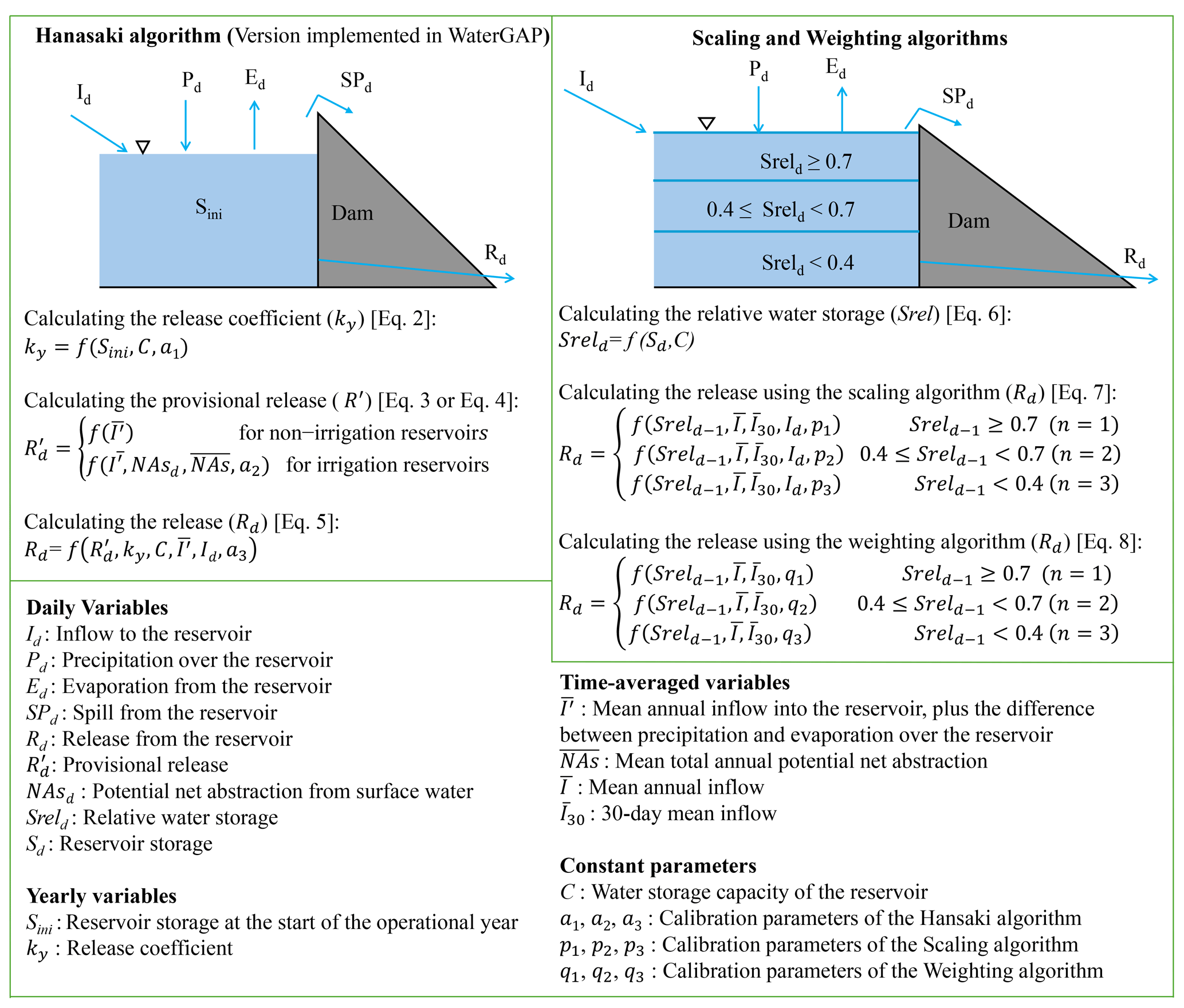
Figure 1 Overview of the process to calculate reservoir release using the Hanasaki (H06), Scaling (SA), and Weighting (WA) algorithms, indicating the required inputs as well as the equation numbers; the complete equations can be found in the text. The left panel details the H06 algorithm implemented in WaterGAP, outlining the steps for calculating the release coefficient, provisional release, and release. The H06 algorithm requires reservoir capacity, storage values at the start of the operational year, daily inflow, precipitation, evaporation data, and daily potential net abstraction data for irrigation reservoirs. The right panel presents SA and WA, indicating the calculation of relative water storage and the release computation as a function of three reservoir water storage levels (n= 1, 2, or 3). SA and WA releases are calculated based on reservoir capacity, daily storage, precipitation, evaporation, and inflow. The time-averaged variables are derived from daily data. For the H06 algorithm DH, the default values for $a_{\mathrm{1}},a_{\mathrm{2}},$ and a₃ are 0.85, 0.5, and 0.5, respectively.

Weighting algorithm

The WA is the same as SA method in most parts of the release calculation; however, in contrast to the SA method, WA does not consider I_d to compute the release and solely relies on Srel_d for weighting $\stackrel{\mathrm{‾}}{I}$ and ${\stackrel{\mathrm{‾}}{I}}_{\mathrm{30}\mathrm{d}}$. Therefore, the contribution of long-term inflow is higher at higher storage levels, while its contribution decreases as storage levels decrease. Conversely, the contribution of inflow from the last 30 d increases as storage decreases. A maximum of 30 % of ${\stackrel{\mathrm{‾}}{I}}_{\mathrm{30}\mathrm{d}}$ contributes to release estimation at higher storage levels (Srel ≥0.7), while it reaches 100 % when the reservoir is empty, which is identical to run-of-the-river flow. In the WA algorithm, when water storage is at level n, the release is estimated as follows:

$$\begin{array}{}\text{(8)}& R_{\mathrm{d}}=q_n\cdot \left[{\mathrm{Srel}}_{\mathrm{d}-\mathrm{1}}\cdot \stackrel{\mathrm{‾}}{I}+\left(\mathrm{1}-{\mathrm{Srel}}_{\mathrm{d}-\mathrm{1}}\right)\cdot {\stackrel{\mathrm{‾}}{I}}_{\mathrm{30}\mathrm{d}}\right]\mathrm{for}n=\mathrm{1},\mathrm{2},\mathrm{3},\end{array}$$

where q_n is the parameter assigned to storage level n that needs to be determined (see Fig. 1). We opted for ${\stackrel{\mathrm{‾}}{I}}_{\mathrm{30}\mathrm{d}}$ over I_d, assuming that release decisions may rather be based on the past inflow over a more extended period and not on the inflow on just the previous day.

Contrary to the H06 approach, where the release is independent of inflow in reservoirs with large storage capacity relative to the annual inflow (resulting in a constant release throughout the year, see Eq. 5), both new algorithms consider the impact of inflow on release in all reservoirs. This impact varies with different seasons and storage levels, leading to variability in release throughout the year, which is more realistic (see Eqs. 7 and 8). It should be noted that the new algorithms do not distinguish between irrigation and non-irrigation reservoirs; therefore, no water use data are required for their application, making their implementation easier than the H06 algorithm. This is because estimating downstream water demand on a large scale is usually very uncertain, and reservoirs are typically designed for multiple purposes.

In each of the three algorithms, if S_d falls below 10 % of the storage capacity (C), the calculated R_d is adjusted to 0.1⋅R_d if the available water is sufficient; otherwise, the entire S_d will be released. Finally, the reservoir outflow is calculated as follows:

$$\begin{array}{}\text{(9)}& O_{\mathrm{d}}=R_{\mathrm{d}}+S{P}_{\mathrm{d}},\end{array}$$

where O_d (m³ s⁻¹) and SP_d (m³ s⁻¹) are the reservoir outflow and the spill from the reservoir during day “d”, respectively. SP_d is calculated as the difference between S_d and C where S_d exceeds C; otherwise, it is zero.

2.3 Data

The ResOpsUS dataset (Steyaert et al., 2022), which was used to calibrate and evaluate the three algorithms in this study, encompasses daily in situ records of inflow, storage, outflow, elevation, and evaporation for up to 679 US reservoirs. The available data cover the years from 1930 to 2020, determined by the commissioning year of each dam and the availability of data. In this study, data on reservoir inflow (daily), outflow (monthly), and storage (monthly) from 1980 to 2019 were considered, divided into two distinct periods: a calibration phase spanning 1980 to 2009 and a validation phase covering the years 2010 to 2019. Monthly data were computed from daily records, excluding months with more than one week of missing values. Subsequently, we applied filters to the dataset, considering only reservoirs with a minimum data length of 5 years and a minimum reservoir capacity of 0.5 km³ . Additionally, we ensured that there is only one reservoir per 0.5° × 0.5° grid cell and that no negative values are present. This resulted in 100 reservoirs, with 35 having data for storage, inflow, and outflow and 65 having data for storage and outflow only. The minimum number of monthly data values for the 65 (35) reservoirs was 111 (252) for the calibration period and 65 (59) for the validation period. The reservoir storage capacities (C) range from 0.5 to 36.7 km³ based on the GRanD dataset (Lehner et al., 2011). Out of the total 100 reservoirs, nine are irrigation reservoirs. Detailed information on each reservoir is provided in Table S1 in the Supplement.

Using in situ storage data, we derived two additional storage-related variables: the time series of the storage anomaly and estimated storage. These variables can also be estimated using remote sensing data. The storage anomaly time series for each reservoir is calculated by subtracting the mean storage during the calibration period from the in situ storage data for each reservoir. However, the storage anomaly lacks information about the bias term, and calibrating against it can lead to a simulated storage time series that significantly deviates from the observed water storage. Having actual absolute storage is beneficial, as reservoirs are the only surface water bodies for which we can model absolute storage within WaterGAP. To provide an alternative, we calculated the “estimated storage time series”; this term refers to storage values that are not observed directly but are estimated using the storage anomaly and the reservoir capacity C. First, we determined the storage change time series by subtracting the initial month's storage anomaly value from the monthly storage anomaly values. Assuming the reservoir reaches maximum capacity at least once between 1980 and 2009, we calculated the maximum monthly storage change, referred to as Dif_max. We then subtracted Dif_max from the GRanD reservoir storage capacity to estimate the initial water storage for the first month. The estimated storage time series is then obtained by adding the storage changes to this estimated initial water storage. Since the data are monthly, and daily maximum storage is generally higher, we applied a 1.2 scaling factor to Dif_max. This adjustment means that Dif_max used in our calculations is 20 % higher than the initially calculated value. This 20 % increase is derived from the mean difference between the maximum daily storage and the monthly storage observed in 100 studied reservoirs (see Table S1). The calculation of estimated storage can be performed using either absolute storage or the storage anomaly, as the time series of storage changes would remain the same in both cases. An example using GRanD ID 597 (Glen Canyon Dam, Lake Powell) clarifies the calculation of the storage anomaly and estimated storage. The mean observed storage value between 1980 and 2009 for Glen Canyon Dam is 22.45 km³. To obtain the storage anomaly time series for this reservoir, the value of 22.45 km³ is subtracted from all storage data for the reservoir over the entire period (1980–2019). For calculating estimated storage, the Dif_max is 6.6 km³ , which occurred in July 1983 (see Supplement Fig. S1). This is calculated as the storage anomaly value in July 1983 minus the initial storage anomaly value in January 1980. The initial storage is estimated as 25.1 km³ (the reservoir capacity reported by GRanD) minus 7.9 km³ (6.6 km³ × 1.2). This gives an initial storage value of approximately 17.2 km³. Storage changes are then added to the estimated initial storage to obtain the time series of estimated storage (Fig. S1c); e.g., the estimated storage for July 1983 is 23.8 km³ , which is the sum of 17.2 and 6.6 km³.

2.4 Model variants and calibration approach

The three reservoir operation algorithms were implemented in WaterGAP. For each algorithm, the algorithm-specific parameters (a₁, a₂, and a₃ for the CH; p₁, p₂, and p₃ for the SA; and q₁, q₂, and q₃ for the WA) were estimated by optimizing the Kling–Gupta efficiency (KGE) (Kling et al., 2012), including the trend term (see Eq. 10). This optimization was performed through a single-objective calibration against the monthly time series of four variables: outflow, storage, the storage anomaly, and estimated storage (see Sect. 2.3). The parameters of each algorithm were calibrated using a grid search approach. Reservoir outflow and storage time series were simulated for all parameter sets listed in Table S2, and the parameter set corresponding to the highest KGE was selected. The parameter estimation using the storage anomaly and estimated storage serves as the main experiment, as the primary emphasis of this study is on exploring the added value of incorporating the storage anomaly (which facilitate the calibration of reservoir algorithms using remote sensing data in regions where in situ storage time series are unavailable) into the calibration of reservoir operation algorithms.

As in previous studies by Dong et al. (2023), Turner et al. (2021), and Shin et al. (2019), the uncalibrated H06 (DH) is used as a benchmark. For comparison purposes, in all calibration experiments based on WaterGAP inflow, the inflow into reservoirs simulated by the DH algorithm was used to ensure that the same inflow data were applied across all algorithms. To achieve this, WaterGAP was first run with the DH algorithm to save the reservoir inflow data. These inflow data were then read from the saved files and used as the inflow source to model each reservoir independently. As a result, the inflow into all reservoirs, regardless of their position, was based on the DH algorithm when applying the CH, SA, and WA algorithms, meaning that the operations of upstream reservoirs did not affect those of downstream reservoirs. The calibration runs were initialized by running WaterGAP five times for the year 1979, allowing water storage to reach a relatively stable equilibrium state.

In addition to the inflow simulated by WaterGAP, we also assessed the algorithms based on observed inflow where available. This was done to evaluate the performance of reservoir operation algorithms in the presence of high-quality inflow data, as poor inflow data can significantly impact the performance of these algorithms (Vanderkelen et al., 2022). Moreover, we assessed the impact of distinguishing irrigation and supply reservoirs from other reservoirs. The distinction for irrigation reservoirs is the default approach for the H06 algorithm; however, here we also applied this distinction for supply reservoirs, as their outflow also depends on downstream demand. To this end, we modeled 21 reservoirs (nine irrigation and 12 supply reservoirs) in two different ways for all algorithms: one that included downstream demand and the other that did not consider it. The purpose of this comparison is to evaluate whether including downstream demand, despite the high uncertainty in water demand estimation for the reservoirs, enhances the outflow and storage simulation or whether it adds value without introducing unnecessary complexity. In the case of the SA and WA approaches for considering downstream demand, the process involves using the provisional release $R_{\mathrm{d}}^{\prime }$ instead of $\stackrel{\mathrm{‾}}{I}$ in Eqs. (7) and (8). Therefore, similar to the DH algorithm, Eq. (4) was used with the default value for the parameter a₂ to estimate $R_{\mathrm{d}}^{\prime }$. Please note that, since the WA and SA approaches work with $\stackrel{\mathrm{‾}}{I}$ and not $\stackrel{\mathrm{‾}}{I^{\prime }}$, $\stackrel{\mathrm{‾}}{I}$ was applied in Eq. (4) instead of $\stackrel{\mathrm{‾}}{I^{\prime }}$ in the SA and WA approaches.

Table 1 shows a summary of the different calibration variants. In Table 1, each calibration variant is characterized by a combination of a reservoir operation algorithm, a calibration variable, an inflow source, and whether downstream demand is considered or not. For example, calibrating the CH algorithm against outflow using inflow simulated by WaterGAP while considering downstream water demand represents one calibration variant. Thus, each reservoir operation algorithm comprises 12 calibration variants (eight utilizing WaterGAP inflow and four using observed inflow), leading to a total of 36 calibration variants.

Table 1 Components of the different calibration variants, comprising 36 variants in total, with 12 variants for each algorithm. Each algorithm includes four variants that use WaterGAP inflow with downstream demand considerations (calibrated against outflow, storage, the storage anomaly, and estimated storage), four variants that use WaterGAP inflow without downstream demand, and four variants that use observed inflow. Each calibration variant is defined by the combination of a reservoir operation algorithm, calibration variable, inflow source, and the consideration or non-consideration of downstream demand. For CH, the default approach incorporates the downstream demand of irrigation reservoirs, while the opposite is true for SA and WA. Additionally, considering the downstream demand for supply reservoirs is not the default approach for any of the reservoir operation algorithms. For calibration variants that utilize observed inflow, only the default approach of each algorithm is considered.

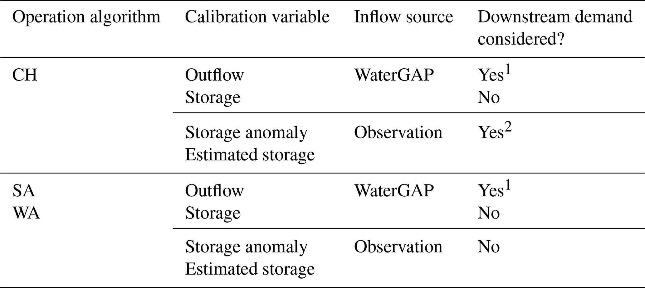
¹ Water demand is considered for irrigation and supply reservoirs, i.e., 21 out of 100 studied reservoirs. ² Water demand is considered for irrigation reservoirs, i.e., 2 out of 35 studied reservoirs with observed inflow.

2.5 Performance evaluation metrics

The performance of the reservoir operation algorithms was evaluated using KGE and the normalized root mean square error (nRMSE). KGE is widely used for model calibration and evaluation, as it simultaneously considers multiple important aspects of model performance, providing a comprehensive assessment (Beck et al., 2019; Lamontagne et al., 2020). The use of nRMSE offers additional insights by focusing on the magnitude of errors. Following Hosseini-Moghari et al. (2020), we incorporated the trend component into the conventional KGE equation as follows:

$$\begin{array}{}\text{(10)}& {\displaystyle }\begin{array}{rl}\mathrm{KGE}=\mathrm{1}-& \sqrt{{\left(R_{\mathrm{KGE}}-\mathrm{1}\right)}^{\mathrm{2}}+{\left(B_{\mathrm{KGE}}-\mathrm{1}\right)}^{\mathrm{2}}}\\ & \stackrel{\mathrm{‾}}{+(V_{\mathrm{KGE}}-\mathrm{1}{)}^{\mathrm{2}}+(T_{\mathrm{KGE}}-\mathrm{1}{)}^{\mathrm{2}}}\end{array}\text{(11)}& {\displaystyle }{R}_{\mathrm{KGE}}={\displaystyle \frac{\mathrm{cov}(\mathrm{sim},\mathrm{obs})}{{\mathit{\sigma }}_{\mathrm{sim}}\cdot {\mathit{\sigma }}_{\mathrm{obs}}}}\text{(12)}& {\displaystyle }{B}_{\mathrm{KGE}}={\displaystyle \frac{\stackrel{\mathrm{‾}}{\mathrm{sim}}}{\stackrel{\mathrm{‾}}{\mathrm{obs}}}}\text{(13)}& {\displaystyle }{V}_{\mathrm{KGE}}={\displaystyle \frac{{\mathit{\sigma }}_{\mathrm{sim}}/\stackrel{\mathrm{‾}}{\mathrm{sim}}}{{\mathit{\sigma }}_{\mathrm{obs}}/\stackrel{\mathrm{‾}}{\mathrm{obs}}}}\text{(14)}& {\displaystyle }{T}_{\mathrm{KGE}}={\displaystyle \frac{T_{\mathrm{sim}}}{T_{\mathrm{obs}}}},\end{array}$$

where R_KGE represents the correlation coefficient between observed (obs) and simulated (sim) time series; B_KGE denotes the bias of the mean simulated ($\stackrel{\mathrm{‾}}{\mathrm{sim}}$) compared to the mean of observed ($\stackrel{\mathrm{‾}}{\mathrm{obs}}$); V_KGE is the variability component that denotes the ratio of the standard deviation of the simulated (σ_sim) to the standard deviation of the observed (σ_obs) time series, divided by their mean; and T_KGE represents the ratio of the linear trend of the simulated time series (T_sim) to the observed one (T_obs). In the case of calibrating against the storage anomaly, we did not divide σ by the mean, as the mean for the storage anomaly is zero. Similarly, the B_KGE component was not considered in calculating KGE related to the storage anomaly. The optimal value for the KGE and its four components is 1. The KGE range is ($-\mathrm{\infty },\mathrm{1}]$, while R_KGE ranges from −1 to 1; B_KGE, V_KGE, and T_KGE can vary between −∞ and +∞. Following Knoben et al. (2019), a KGE value above −0.73 indicates that the model performs better than the mean of observations if the trend component is included in the KGE.

The normalized root mean square error (nRMSE) is calculated as

$$\begin{array}{}\text{(15)}& \mathrm{nRMSE}={\displaystyle \frac{\sqrt{\frac{\mathrm{1}}{T}{\sum }_{t=\mathrm{1}}^T({\mathrm{obs}}_t-{\mathrm{sim}}_t{)}^{\mathrm{2}}}}{{\mathit{\sigma }}_{\mathrm{obs}}}}.\end{array}$$

The perfect value for nRMSE is zero. Normalizing the RMSE with the standard deviation of observations brings this metric closer to the Nash–Sutcliffe efficiency (NSE), but different from the NSE, the nRMSE cannot become negative (Turner et al., 2021).

3 Results

3.1 Performance of calibration variants in the case of simulated inflow into reservoirs

We found that calibrating against observed water storage, the water storage anomaly, or estimated water storage (derived from the storage anomaly and GRanD capacity) improves the very poor simulation of storage by the calibration-free algorithm (DH) during both calibration and validation for all three algorithms (Table 2). In the case of DH, storage simulation is skillful, i.e. with a KGE_storage > −0.73 for only 16 % of the 100 reservoirs in the calibration period and 15 % in the validation period. Calibration of the H06 reservoir operation algorithm (CH) achieves skillful storage simulations for 64 % (39 %) of the reservoirs when calibrated against the storage anomaly and for 69 % (32 %) of the reservoirs when calibrated against estimated storage during the calibration (validation) period. Both SA and WA perform better than CH in storage simulation when calibrated against storage-related variables for the calibration and validation periods (Table 2 and Fig. 2). However, the fit of simulated to observed storage remains poor during the validation period, particularly after calibration against the storage anomaly and estimated storage (Table 2 and Fig. 2).

Table 2 The number of reservoirs out of 100 in which KGE values are greater than the benchmark thresholds of −0.73 during the calibration (validation) phase. All algorithms were calibrated against outflow, storage, the storage anomaly, and estimated storage, using KGE as the objective function. The inflow data are sourced from the WaterGAP model.

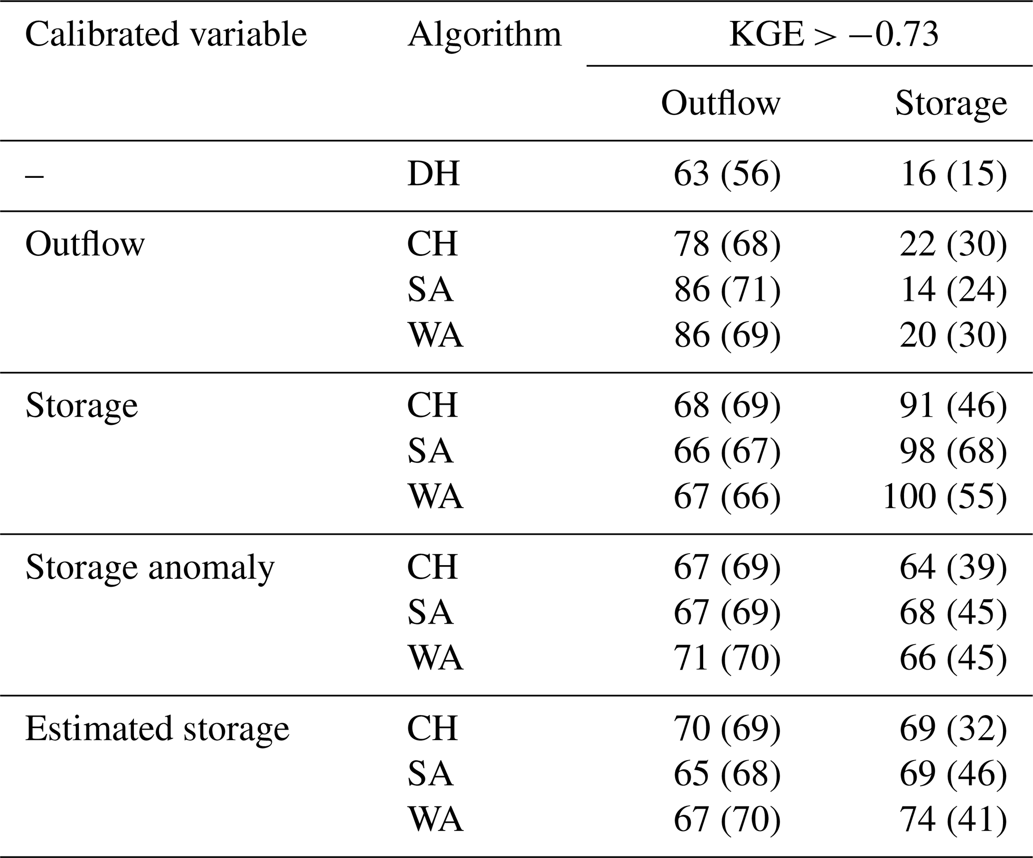
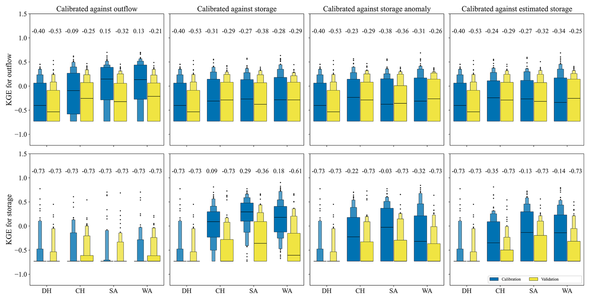
Figure 2 Letter-value plots of KGE for outflow and storage of 100 studied reservoirs for DH, CH, SA, and WA algorithms for the calibration period (1980–2009, in blue) and validation period (2010–2019, in yellow). All algorithms are calibrated against outflow (first column), storage (second column), the storage anomaly (third column), and estimated storage (fourth column), using KGE as the objective function. The values at the top of the panels are the median KGE (indicated by the horizontal line). KGE values below the benchmark threshold of −0.73 are set to −0.73. The widest box contains 50 % of the 100 data points, the second widest 25 % of the data (12.5 % in the upper box and 12.5 % in the lower box), the third widest 12.5 %, and so on. The inflow data are sourced from the WaterGAP model.

Calibrating for storage-related variables only slightly improves the mostly poor simulations of reservoir outflow during the calibration period, with slightly better outcomes observed in the validation period (Table 2 and Fig. 2). Skillful outflow simulations were achieved for 86 % of the reservoirs when either SA or WA was calibrated against outflow, compared to 78 % for CH and 63 % for DH during the calibration phase. However, skillful storage simulations were observed in only 14 % (24 %) and 20 % (30 %) of the reservoirs for SA and WA, respectively, compared to 22 % (30 %) for CH and 16 % (15 %) for DH in the calibration (validation) phase (Table 2). The performances of outflow simulations with CH, SA, and WA are very similar during both the calibration and validation periods, except when calibrating against observed outflow in the calibration period. In this case, SA and WA achieved positive KGE_outflow, with medians of 0.15 for SA and 0.13 for WA. Calibrating with respect to outflow improves the correlation, variability, and trend of the simulated outflow relative to DH across all three algorithms, while the bias remains largely unchanged (Figs. S2–S5). On average, outflow trends are underestimated. Calibrating against outflow worsens both the correlation and variability of storage simulations across all three algorithms during the calibration phase, though it notably improves the bias component (Figs. S2–S4). Model performance related to storage is not affected in a relevant manner by calibration against outflow and remains very poor. When algorithms are calibrated against outflow, the mean observed storage is usually a better estimator than the simulated storage.

Calibrating against storage (Fig. 2, second column) yields the highest KGE_storage values, with a median of 0.29, and SA outperforms CH and WA, while KGE_outflow and its component values across the three algorithms are similar (Figs. S2–S5). Calibration against the storage anomaly (third column in Fig. 2) or estimated storage (fourth column in Fig. 2) improves both storage and outflow simulations compared to DH, but the fit to observed storage is worse than calibration against storage. The median KGE_storage for calibration against the storage anomaly exceeds that for estimated storage, yet the letter-value plot shows the widest box for estimated storage, indicating 50 % of the data are above that for the storage anomaly. Storage simulation improvement largely stems from bias adjustment (Fig. S3). The DH algorithm shows a median B_KGE of 1.90 during calibration, dropping to 0.92 (1.04, 0.99), 0.71 (0.91, 1.18), and 1.25 (1.44, 1.32) for calibrating against storage, the storage anomaly, and estimated storage of the CH (SA, WA) algorithms. Correlation improves for SA and WA only during calibration (Fig. S2). Variability improves when calibrating against the storage anomaly, whereas estimated storage underestimates variability (Fig. S4). Trends of KGE_storage improve significantly when calibrating against storage, the storage anomaly, and estimated storage compared to DH, though trends are generally underestimated (Fig. S5). Evaluating KGE_{storage_anomaly} with different variables shows less degradation in the validation phase (Fig. S6). For instance, skillful simulations for storage reached 17 (18), 93 (44), 98 (59), and 99 (55) for DH, CH, SA, and WA, respectively, when calibrated with storage anomalies (see Table 2 for comparison). The fit to observed storage variables is less improved for validation than calibration (Table 2, Fig. 2). Comparing calibration against the storage anomaly and estimated storage shows SA and WA are preferred over CH and DH, even though the differences from CH are minor during validation. Differences between KGE_storage values of SA and WA are small for all calibration variables in both calibration and validation periods.

Examining the empirical cumulative distribution functions (eCDFs) for nRMSE reveals that the eCDFs for outflow are much closer across algorithms than those for storage (see Fig. 3). This implies calibration has a more significant impact on storage than on outflow. Calibrating against any storage-related variable generally enhances outflow performance at lower nRMSE_outflow levels in about 60 % of reservoirs. In comparison, at higher levels, a slight degradation occurs in roughly 35 % of reservoirs (with probabilities between 0.60 and 0.95). When calibrating against outflow, nRMSE_storage generally improves for CH and WA algorithms, but no clear enhancement is seen for SA. Additionally, the nRMSE_outflow decreases for over 40 % of reservoirs. For nRMSE_outflow greater than 0.98, calibration against outflow shows nearly no improvement, as indicated by the eCDFs. Calibration against the storage anomaly, the main calibration variant, especially in the validation phase, reveals that SA slightly outperforms WA, with lower nRMSE_storage and similar nRMSE_outflow. Regardless of the magnitude of the error, the eCDF for validation exhibits a shape similar to that of the calibration period, indicating that the error distribution for the algorithm remains consistent across both periods.

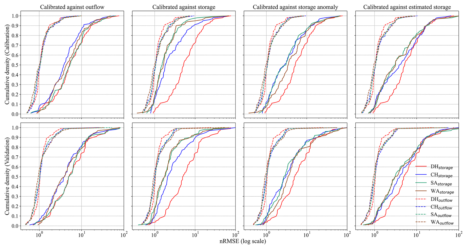
Figure 3 Empirical cumulative distribution functions of nRMSE for storage and outflow of the 100 studied reservoirs are based on the DH, CH, SA, and WA algorithms for the calibration period (1980–2009) and the validation period (2010–2019). All algorithms are calibrated against outflow (first column), storage (second column), the storage anomaly (third column), and estimated storage (fourth column), using KGE as the objective function. The x axis uses a logarithmic scale. If nRMSE is greater than 1, the mean error exceeds the standard deviation of the observational values. The inflow data are sourced from the WaterGAP model.

3.2 Illustrative calibration results for three reservoirs

As an example, we plotted the time series of storage and outflow for the Glen Canyon Dam (Lake Powell) in Figs. 4 and S7, respectively. Results for this reservoir suggest that calibrating the H06 algorithm based on outflow did not yield better outcomes than the DH model (Figs. 4a, S7a). Some improvement was noted in the outflow simulation for SA and WA during calibration; however, this resulted in a worse simulation during validation (Fig. S7). Despite this, with a KGE > −0.73, all outflow simulations demonstrated skillful performance. Calibration against outflow did not negatively impact storage simulation relative to the DH, except for SA, particularly during validation, where the variability of the simulated series was over 3 times higher than the observed values (Table S3). During the calibration phase against storage-related variables, simulated storage levels primarily exceed 40 % (10 km³) of the total capacity. This pattern results in storage levels under 40 % being inadequately handled during the parameter selection for the SA and WA algorithms. Consequently, when storage levels drop below 10 km³ during the validation phase, the outcomes are not promising (Fig. 4c, d). Furthermore, the discrepancy between the reported capacity by GRanD (25 km³) and the maximum recorded daily storage (31.7 km³) negatively impacts the simulation outcomes for all calibrated algorithms that rely on estimated storage versus storage anomalies (see Fig. S1). This approximately 20 % discrepancy between the reported capacity and the maximum observed storage introduces a bias, which influences the bias and variability components of KGE_storage (Table S3). The outflow shows almost no bias due to the use of data from the Lees Ferry station, located just downstream of the dam, for bias adjustment in WaterGAP's streamflow simulations via a simple calibration approach (see Müller Schmied et al., 2024, for more details).

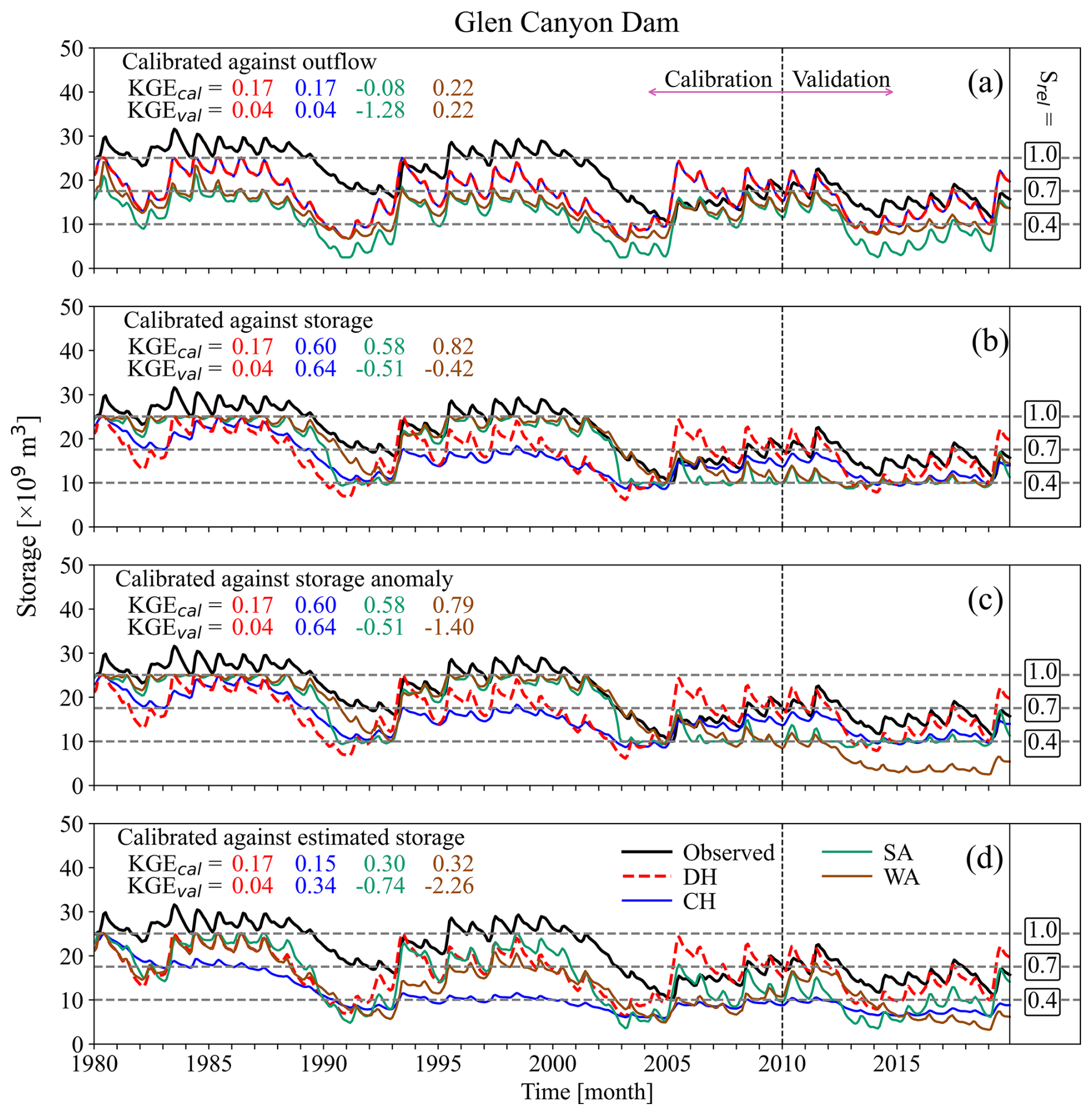
Figure 4 Monthly time series of observed and simulated storage values from DH, CH, SA, and WA algorithms for Glen Canyon dam, GRanD ID 597, calibrated against (a) outflow, (b) storage, (c) the storage anomaly, and (d) estimated storage using KGE as the objective function. The dashed black lines distinguish between the calibration and validation periods. The dashed gray lines indicate the relative storage levels (S_rel), categorizing GRanD storage into three categories: above 70 % of storage capacity, between 40 % and 70 % of storage capacity, and below 40 % of storage capacity for the reservoir. The maximum observed storage (31.7 km³) exceeds the capacity reported in the GRanD dataset (25 km³). The inflow data are sourced from the WaterGAP model. The time series for outflow is plotted in Fig. S7.

The storage simulation for the Yellowtail Dam (an irrigation reservoir, GRanD ID = 355) and the Harry S. Truman Dam (a hydropower reservoir, GRanD ID = 989) is poor, with a higher seasonal magnitude compared to the observed data. (Fig. 5). Calibrating using the storage anomaly can introduce significant bias in absolute storage simulation (Fig. 5c). Similarly, calibrating with estimated storage may cause issues if there is a mismatch with in situ observations (Fig. 4d). For the Yellowtail Reservoir, SA and WA, which do not account for downstream water demand, simulate storage more accurately than DH and CH, which consider downstream water demand (Fig. 5a). However, for outflow simulation, the uncalibrated DH performs the best (Fig. S8a).

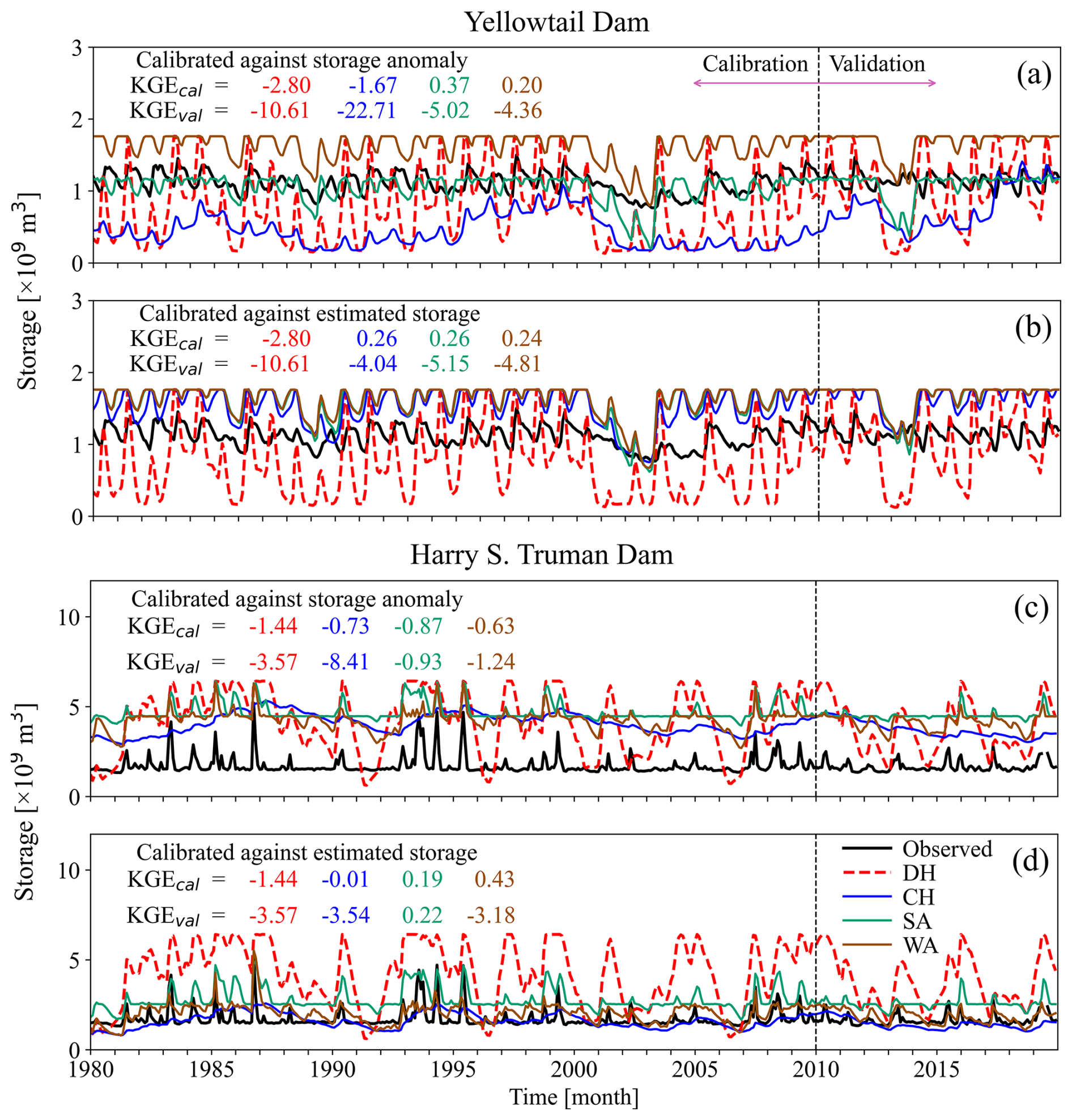
Figure 5 Monthly time series of observed and simulated storage values from DH, CH, SA, and WA algorithms for Yellowtail/Harry S. Truman reservoirs, GRanD IDs $\mathrm{355}/\mathrm{989}$, calibrated against (a, c) the storage anomaly and (b, d) estimated storage using KGE as the objective function. The primary purposes of the Yellowtail Dam and the Harry S. Truman Dam are irrigation and hydropower, respectively. The dashed black lines distinguish between the calibration and validation periods. The inflow data are sourced from the WaterGAP model. The time series for outflow is plotted in Fig. S8.

These examples show that calibrating only against storage variables does not necessarily worsen outflow simulations (Fig. S8). However, attention to inaccuracies in reservoir capacity data in the GRanD dataset is critical when evaluating reservoir operation performance. In these cases, comparing storage anomalies may provide a more accurate assessment than relying solely on absolute storage. This storage simulation error may also impact outflow simulations, where input data inaccuracies primarily lead to incorrect storage levels during the validation phase (Fig. 4c).

3.3 Impact of using observed streamflow as input to the reservoir operation algorithms

The comparison of modeling results using WaterGAP inflow and observed inflow is shown in Fig. 6 for 35 out of the 100 studied reservoirs. Figure 6 shows no considerable change in storage simulation with either observed or WaterGAP inflow data, except for the WA algorithm, which performs better with observed inflow than with simulated inflow (Fig. 6c). Nonetheless, the performance of WA in storage simulation with observed inflow does not exceed that of SA. Conversely, using observed inflow data considerably enhances the reservoir outflow simulation. For instance, KGE_outflow below −1 achieved with WaterGAP inflow can approach 1 with observed inflow (Fig. 6f). In most cases, KGE_outflow between 0–0.5 based on WaterGAP inflow reaches 0.5–1 based on observed inflow. The most substantial improvement is seen in the WA algorithm, where the median of KGE_outflow across various calibration objectives, ranging from [−0.27, 0.14], rises to [0.56, 0.69] upon replacing WaterGAP inflow with observed data. This implies that the WA is more sensitive to the quality of inflow data than other algorithms. During the validation period, the same pattern is repeated, showing a median KGE_outflow of [0.38, 0.56] compared to [−0.87, −0.41], based on observed inflow versus WaterGAP inflow across all calibration variants (Fig. S9). Utilizing the observed inflow enhances nearly all components of KGE_outflow, with the most notable improvements seen in the variability and trend components (see Figs. S10–S17).

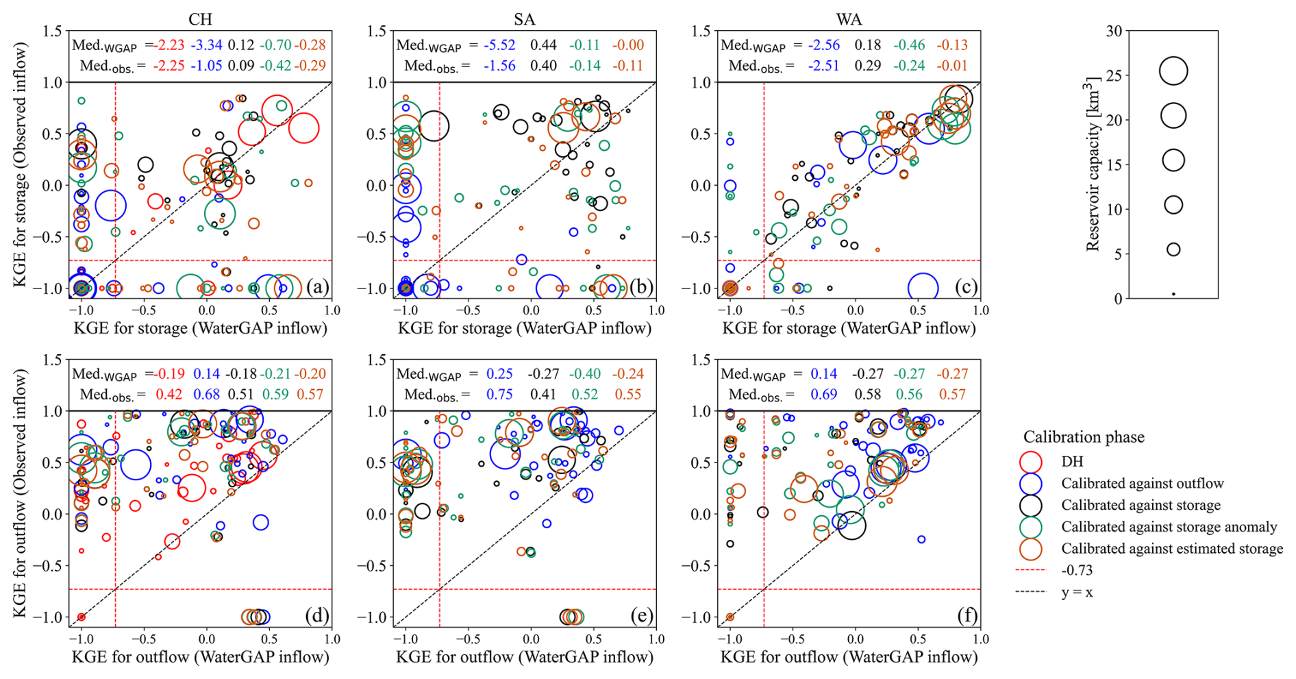
Figure 6 The relationship between the KGE of (a)–(c) storage and (d)–(f) outflow is obtained from modeling reservoirs using WaterGAP inflow and the observed inflow to the reservoirs during the calibration period (1980–2009) for 35 reservoirs with observed inflow. KGE values less than −1 are set to −1. The KGE values for the storage anomaly and estimated storage are not displayed. The size of the circles indicates the reservoir capacity. The values above each panel show the median KGE, with the top values achieved with WaterGAP inflow and the bottom values derived from observed inflow. The dashed red lines represent the KGE benchmark threshold of −0.73.

3.4 Impact of considering downstream water demand

We assessed the advantages of differentiating irrigation and water supply reservoirs from others by counting how many times estimating the outflow of irrigation reservoirs (9 reservoirs) and supply reservoirs (12 reservoirs) using Eq. (4) results in a more accurate simulation compared to ignoring water demand in the modeling of reservoir dynamics. We found that there is no general advantage in distinguishing irrigation and supply reservoirs from other reservoirs, particularly when calibrating against the storage anomaly or estimated storage using the overall superior WA and SA algorithms. In terms of calibration against estimated storage, the SA algorithm performs better for outflow when considering downstream demand; however, the opposite is true for storage. In the WA algorithm, the same number of reservoirs achieves better or worse streamflow performance when downstream water demand is considered. However, storage performance is enhanced when demand is disregarded (Table 3).

Table 3 Comparison of reservoir simulation performance using different algorithms, both with and without considering downstream water demand for 21 irrigation and supply reservoirs. Numbers outside parentheses indicate the number of reservoirs (out of 21) where performance improves when downstream demand is taken into account. In contrast, values inside parentheses represent reservoirs where ignoring downstream demand leads to higher KGE values. Improvements are noted only for skillful simulations achieving a KGE value greater than −0.73. All algorithms are calibrated against outflow, storage, the storage anomaly, and estimated storage using KGE as the objective function. The inflow data are sourced from the WaterGAP model.

4 Discussion

4.1 Calibration variables

Calibrating against outflow does not necessarily improve storage simulations and may even cause their deterioration during the calibration phase. In contrast, calibrating against all types of storage-related variables slightly improves outflow compared to the DH algorithm (see Fig. 2 and Table 2). Thus, calibrating against storage-related variables is more effective than calibrating against outflow when aiming to improve the simulation of both variables through a single-objective calibration. Furthermore, an analysis of the KGE values for the compromise solution – defined as the one with the smallest Euclidean distance from the ideal KGE value of 1 for both storage and outflow – reveals that the KGE results from calibration against storage are considerably closer to the compromise solution than those for outflow (refer to Fig. S18). A similar pattern is seen in calibrations against both the storage anomaly and estimated storage. One reason for this is that outflow simulations are less sensitive to calibration compared to storage simulations. This finding is encouraging because, unlike outflow data, the storage anomaly can be estimated using remotely sensed data. The data length should exceed 5 years to be used effectively for this purpose (Otta et al., 2023). Although our results indicate that, in general, calibrating against the storage anomaly improves the simulation of storage, using the absolute simulated storage from these calibrations should be approached with caution, as they do not always ensure an improvement in absolute storage.

Calibrating against estimated storage does not outperform calibrating against the storage anomaly (see Fig. 2 and Table 2). Although theoretically, it should yield results closer to those of calibrating against actual storage. The reason, aside from inherent storage estimation errors, lies in the discrepancies between GRanD's capacity data and the maximum daily recorded storage, with a median difference of about 25 % (refer to Table S1). Steyaert and Condon (2024) also reported that GRanD's omission of overtopping and potential inaccurate data led to 100 of the 679 dams in the ResOpsUS dataset having maximum storage values exceeding the reservoir capacities reported by GRanD. Inconsistencies are also reported for the reservoir area; Dong et al. (2023) indicated that the actual polygons of Ertan and Jinping I reservoirs are 69 % and 50 % larger, respectively, than the GRanD polygons. Consequently, simulating the operation of reservoirs that have inaccurate GRanD data are unlikely to yield favorable results, especially in terms of absolute storage simulation. Thus, an absolute storage comparison may not be a fair approach for assessing model performance, although it still holds validity for comparing different algorithms. An evaluation of the degradation in KGE values, comparing calibration against estimated storage with calibration against actual storage, indicates that the results from estimated storage align closely with those from actual storage when the discrepancy between the reservoir capacity reported by GRanD and the maximum daily observed storage is minimal. As this difference increases, the discrepancy between the results of the two calibration variants also grows (Fig. S19). It is important to note that calibrating against the storage anomaly does not show a direct relationship with these differences in storage.

To the best of our knowledge, there are currently two global datasets – the Global Reservoir Storage (GRS) introduced by Li et al. (2023) and the GloLakes dataset by Hou et al. (2024) – that provide monthly time series of estimated absolute storage using remotely sensed information, along with either a geostatistical model or a volume–elevation/area–volume relationship. We evaluated the quality of their estimates for the absolute storage of the studied reservoirs. GRS covers all 100 studied reservoirs, while GloLakes includes only 57 of those reservoirs. The median KGE_storage (without the trend component) was 0.26 for GRS and 0.14 for GloLakes, showing that neither dataset offers reliable estimates for calibrating reservoir operation algorithms based on absolute storage (see Table S4). The B_KGE components for GRS exhibit a median of 0.84, varying from marked underestimation – for example, at Norfork Dam (GRanD ID 1042), the average estimated storage is merely 2 % of the observed value – to considerable overestimation, as seen at Albeni Falls Dam (GRanD ID 305), where the average estimated storage is 45 times the observed value. GloLakes, with a median B_KGE of 1.49, performs slightly better in terms of extreme bias; the most considerable underestimation occurs at Santa Rosa Dam (GRanD ID 1086), where the mean estimated storage is only 35 % of the observed value. The maximum overestimation for GloLakes is observed at the same dam (Albeni Falls Dam), but it is less extreme compared to GRS, although still substantial. The R_KGE and V_KGE components of KGE for storage are better than B_KGE in terms of extreme values. Nonetheless, with medians of 0.63 and 0.84 for GRS and 0.71 and 0.47 for GloLakes, respectively, R_KGE and V_KGE for both datasets are still not sufficiently promising, indicating uncertainty in estimates of remotely sensed storage anomalies.

4.2 Value of calibration and choice of reservoir operation algorithm

Using streamflow from the global hydrological model WaterGAP 2.2e as inflow to 100 US reservoirs, we found that the outflow generated by the calibration-free algorithm DH is a better alternative to the mean observed outflow. Conversely, the opposite holds for simulated reservoir storage (see Fig. 2), highlighting the need for reservoir-specific calibration. Our findings show all three calibrated algorithms generally perform better than DH for storage, but their effect on reservoir outflow simulation is negligible. Improvements vary substantially between reservoirs, with some showing none, as noted by Turner et al. (2021) with a more complex reservoir operation algorithm. Among calibrated algorithms, SA and WA outperform CH when calibrated against storage-related variables. CH may be preferred over SA and WA for irrigation reservoirs with rather good water demand data or if computational resources are very limited, as it estimates only two parameters instead of three for non-irrigation reservoirs. Although KGE cannot distinguish the performance of SA and WA, nRMSE suggests that SA performs slightly better when calibrated against the storage anomaly (Fig. 3).

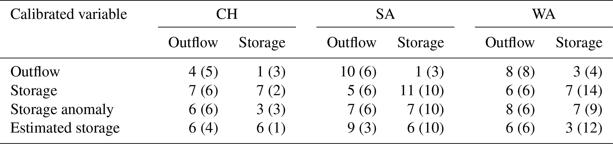
Calibration of H06 shows that default parameters are rarely included in the calibrated sets (Fig. S20), particularly for irrigation reservoirs, where parameter a₂ almost always remains at the lower bound of 0.1. According to Eq. (4), this suggests that calibration emphasizes the use of a scaled version of long-term inflow instead of directly integrating demand through addition. The demand estimation is not accurate enough for reservoir operations, which increases complexity with limited benefits when distinguishing irrigation and supply reservoirs from other types of reservoirs (Table 3). Vanderkelen et al. (2022) similarly observed minimal additional value in incorporating irrigation demand into the reservoir operations.

4.3 Relevance of the quality of simulated reservoir inflow and reservoir storage capacity data

We found that inflow data quality is more crucial than reservoir operation algorithms for outflow simulation but has less impact on storage simulation. This finding aligns with Vanderkelen et al. (2022), who attributed the similar performance of natural lake parameterization and H06 to poorly simulated streamflow in the Community Land Model. Comparing observed inflow as a substitute for simulated outflow and observed outflow shows that the DH algorithm generates worse outflow simulations compared to ignoring the dam. DH has median KGE_outflow values of 0.42 (calibration) and 0.02 (validation), while observed inflow shows median KGE_outflow values of 0.57 (calibration) and 0.36 (validation). This aligns with Vora et al. (2024), who reported that ignoring reservoirs in modeling may lead to better outflow simulations than DH in some cases. However, some skill is observed in other algorithms, particularly SA, where the median KGE_outflow values for CH, SA, and WA are 0.68 (0.46), 0.75 (0.52), and 0.69 (0.56) for calibration (validation), respectively, when calibrated against outflow (see Figs. 6 and S9). Unlike Vanderkelen et al. (2022), our study showed that observed inflow did not significantly improve storage simulation. This may be due to errors in GRanD data, which has a median difference of about 14 % from the maximum daily observed storage for reservoirs with observed inflow data. Another possible reason might be the influence of initial storage on simulation results, which differs based on the regulatory level of reservoir operations, as stated by Yassin et al. (2019). In summary, our results suggest that enhancing the quality of inflow data is more crucial than calibrating reservoir operation algorithms, particularly when the objective is to achieve accurate outflow simulation. Only calibrating against storage anomalies does not ensure better outflow predictions.

4.4 Complexities of reservoir operations and dynamics

Besides poor inflow data and inaccurate capacity information, other factors also affect the performance of reservoir operation algorithms. Incorporating human decision-making into the model is very challenging, despite its critical importance (Rougé et al., 2021). This complexity arises because human decisions do not always follow operational rules due to changing conditions, such as variations in water demand (Shah et al., 2019) or during droughts and floods (Nazemi and Wheater, 2015). For example, the Hoover Dam (Lake Mead) and Glen Canyon Dam (Lake Powell) are interconnected, and historically, Glen Canyon could release enough water to meet downstream needs until 2014. However, due to a drought in 2012 and 2013, releases from Glen Canyon Dam in 2014 dropped to the lowest level since the initial filling of Lake Powell in 1963 (Radonic et al., 2013; U.S. Bureau of Reclamation, 2019). This reduction in release aimed to recover Lake Powell's storage, which had fallen to around 40 % of its capacity (NASA Earth Observatory, 2014). Additionally, climate change and increases in water demand can result in non-stationary situations, meaning that calibrated algorithms may not perform as well compared to the calibration period. This trend is observed in the ResOpsUS dataset, where there is a generally decreasing trend in reservoir storage, which also impacts release (Steyaert and Condon, 2024). For example, the Hoover Dam has experienced a continuous negative trend in its storage since 2000 (see Fig. S21). Understanding these trends is crucial for assessing the degradation of the studied algorithms during the validation period, where the connection between observed inflow and outflow also becomes weaker.

4.5 Limitations

This study modeled reservoirs independently, which may have potentially affected analysis quality. A calibrated upstream reservoir can alter inflows to the downstream reservoir. Nevertheless, as the calibration has not significantly influenced the outflow simulation, it is expected that the overall conclusions will remain comparable. In the case of the SA and WA algorithms, a reservoir might attain relative storage levels (refer to Eqs. 7 and 8) during the validation phase that were not observed during the entire calibration period. As a result, the parameters for these unobserved relative storage levels remain indeterminate and are assigned the minimum value (0.1 for both SA and WA). As a result, the performance of the algorithm for those reservoirs during the validation phase is influenced by setting these undetermined parameters to their lowest value. In the case of the SA algorithm, this issue affects at most four reservoirs across the calibration variants, while for the WA algorithm, it impacts up to nine reservoirs (see Table S5). Yassin et al. (2019) indicate that a 5-year spin-up period is generally sufficient for complete stabilization, even for large dams. In our study, we conducted five simulations of 1979 as our spin-up period. However, using a longer spin-up duration before 1980 could result in different initial storage conditions. Consequently, this might affect the performance of the operational algorithm. These potential limitations should be acknowledged, as they may influence the accuracy and generalizability of the results.

5 Conclusions

This study assessed whether monthly time series of observed reservoir storage anomalies, available globally via remote sensing, are suitable targets for calibrating reservoir operation algorithms in large-scale hydrological models. To accomplish this, we incorporated the well-established Hanasaki algorithm along with two new ones, namely, WA and SA, into the global hydrological model WaterGAP. We calibrated them against the storage anomaly, estimated storage, storage, and outflow data from ResOpsUS for 100 US reservoirs. For 35 of these reservoirs with observed inflow data, both observed and simulated inflows were included in the analysis. Our findings lead to the following conclusions:

• Using observed storage-related variables, i.e., the storage anomaly, estimated storage, or storage, to calibrate reservoir algorithms results in a clear improvement in storage simulation and slightly enhances outflow simulation during calibration, especially against storage. However, the performance of the algorithms for storage during validation is still inferior to that for outflow. Calibration with scarce outflow data improves only the simulated outflow, leaving the simulated storage distinctly poor.

• Of the three calibrated reservoir operation algorithms, the two new algorithms, WA and SA, perform similarly or better in storage simulation than CH, i.e., the calibrated Hanasaki algorithm.

• If observations of either storage, the storage anomaly, or outflow are available for a reservoir, the parameters of the reservoir algorithm should be adjusted, as we found that the default parameter set of the DH algorithm, particularly the irrigation reservoir parameter, is seldom the optimal set. For reservoirs without observations, a calibration-free algorithm such as DH has to be used.

• Modeling irrigation and supply reservoirs with water demand, as in DH, may not enhance reservoir simulation due to uncertainty in demand estimation. We recommend ignoring downstream water demand for these reservoirs.

• We found that using observed inflow instead of simulated inflow considerably improves the performance of the reservoir operation algorithms regarding outflow simulation, although it has minimal impact on their performance in storage simulation.

• For many reservoirs, none of the three relatively simple reservoir operation algorithms can accurately depict the dynamics of both outflow and storage, despite calibration with observations of outflow or storage-related variables and using observed inflow in the simulation. The complexity of human decision-making eludes algorithms that rely solely on globally available information, even when parameters are adjusted through calibration.

• To enhance large-scale hydrological modeling, we recommend utilizing recent and upcoming spaceborne data on reservoir water storage anomalies by employing the SA or WA reservoir operation algorithms. These algorithms facilitate reservoir-specific calibration against observed storage anomalies. After calibration, they demonstrated slightly improved performance over the CH algorithm and are more suited for large-scale applications compared to algorithms like those from Chen et al. (2022) and Turner et al. (2021), which require daily inflow, storage, and outflow data – information that is seldom accessible outside the US.

• Due to the strong biases often exhibited by the currently available time series of absolute reservoir storage derived from the remote-sensing-based water storage anomaly, and considering that calibration against estimated storage does not outperform calibration against the storage anomaly, we recommend estimating the parameters of the SA or WA algorithm using globally available, remote-sensing-based monthly time series of the reservoir water storage anomaly (and in situ storage and outflow time series where available). This approach is expected to particularly enhance the quality of simulated reservoir storage.

Although the algorithms introduced in this study outperform the conventional DH algorithm, there remains scope for improvement. For example, integrating knowledge-based equations with deep learning in hybrid machine learning methods could be beneficial for simulating reservoir dynamics. However, improving the accuracy of inflow simulations and validating reservoir-related characteristics is very likely more important for achieving better reservoir outflow and storage simulations than refining the algorithm itself.