Adaptation of root zone storage capacity to climate change and its effects on future streamflow in Alpine catchments: towards non-stationary model parameters

Hydrological models play a vital role in projecting future changes in streamflow. Despite the strong awareness of non-stationarity in hydrological system characteristics, model parameters are typically assumed to be stationary and derived through calibration on past conditions. Integrating the dynamics of system change in hydrological models remains challenging due to uncertainties related to future changes in climate and ecosystems.

Nevertheless, there is increasing evidence that vegetation adjusts its root zone storage capacity – considered a critical parameter in hydrological models – to prevailing hydroclimatic conditions. This adaptation of the root zone to moisture deficits can be estimated by the Memory method. When combined with long-term water budget estimates from the Budyko framework, the Memory method offers a promising approach to estimate future climate–vegetation interaction and thus time-variable parameters in process-based hydrological models.

Our study provides an exploratory analysis of non-stationary parameters for root zone storage capacity in hydrological models for projecting streamflow in six catchments in the Austrian Alps, specifically investigating how future changes in root zone storage impact modeled streamflow. Using the Memory method, we derive climate-based parameter estimates of the root zone storage capacity under historical and projected future climate conditions. These climate-based estimates are then implemented in our hydrological model to assess the resultant impact on modeled past and future streamflow.

Our findings indicate that climate-based parameter estimations significantly narrow the parameter ranges linked to root zone storage capacity. This contrasts with the broader ranges obtained solely through calibration. Moreover, using projections from 14 climate models, our findings indicate a substantial increase in the root zone storage capacity parameters across all catchments in the future, ranging from +10 % to +100 %. Despite these alterations, the model performance remains relatively consistent when evaluating past streamflow, independent of using calibrated or climate-based estimations for the root zone storage capacity parameter. Additionally, no significant differences are found when modeling future streamflow when including future climate-induced adaptation of the root zone storage capacity in the hydrological model. Variations in annual mean, maximum and minimum flows remain within a 5 % range, with slight increases found for monthly streamflow and runoff coefficients. Our research shows that although climate-induced changes in root zone storage capacity occur, they do not notably affect future streamflow projections in the Alpine catchments under study. Our findings suggest that incorporating a dynamic representation of the root zone storage capacity parameter may not be crucial for modeling streamflow in humid and energy-limited catchments. However, our observations indicate relatively larger changes in root zone storage capacity within the less humid catchments, corresponding to higher variations in modeled future streamflow. This suggests a potentially higher importance of dynamic representations of root zone characteristics in arid regions and underscores the necessity for further research on non-stationarity in these regions.

1 Introduction

Climate change is expected to further increase global temperature and precipitation extremes in the future, thereby causing the hydrological cycle to accelerate (IPCC, 2023). In combination with direct land-use change by humans (e.g., deforestation), climate change affects vegetation and its crucial role in the terrestrial water cycle through changes in overall plant biomass, species distribution and water use efficiency (Stephens et al., 2021). While difficult to generalize, there has been recent progress in quantitatively describing the effect of deforestation and reforestation on the hydrological response with time-variable parameterizations of hydrological models (e.g., Zhang et al., 2017; Teuling et al., 2019; Nijzink et al., 2016; Hrachowitz et al., 2021). In contrast, the natural adaptation of ecosystems to a changing climate remains less understood due to its gradual, long-term nature – unlike the more abrupt impacts of human-induced land-use change (Seibert and van Meerveld, 2016) – and the complex feedbacks among soils, vegetation and climate (Stephens et al., 2021). The complexity of natural ecosystem adaptation is further emphasized in a recent debate regarding whether ecosystem responses to climate primarily shape soil and subsequently influence water flow (Gao et al., 2023, or, conversely, whether water flow is the dominant force shaping soil characteristics (Zhao et al., 2024). These characteristics of the natural adaptation of ecosystems complicate the reliable prediction of the future hydrological responses of catchments under change, which is recognized as a major challenge in hydrology (Blöschl et al., 2019; Berghuijs et al., 2020).

The quantification of how physical characteristics of a terrestrial hydrological system are affected by climate change is complex. In the absence of that knowledge, model parameters, observed or calibrated to past observations, are typically used for predicting future hydrological responses. However, inferring model parameters from historic conditions requires the implicit assumption that the considered system is stationary and that its physical characteristics (and thus model parameters), such as vegetation root systems, do not change over the modeling period. Although this assumption may hold for predictions on shorter timescales, assuming long-term system stationarity under a changing climate may lead to misrepresentations of the underlying processes and result in considerable associated predictive uncertainties (e.g., Fenicia et al., 2009; Hrachowitz et al., 2021; Bouaziz et al., 2022).

There is increasing evidence that vegetation dynamically adapts its root systems to the prevailing climate in order to guarantee water supply to satisfy the canopy water demand by transpiration (Kleidon, 2004; Schymanski et al., 2009). As such, changes in the root system change the soil pore volume and thus the water volume between the permanent wilting point and field capacity that is within reach and can be accessed by vegetation roots to satisfy water demand in dry periods. This maximum vegetation-accessible water volume is hereafter referred to as the “root zone storage capacity”. Regulating the water supply for vegetation, this root zone storage capacity plays a key role in the partitioning of water fluxes in terrestrial hydrological systems, where it regulates the temporally variable ratio between drainage and evaporative water fluxes (Rodriguez-Iturbe et al., 2007; Savenije and Hrachowitz, 2017; Oorschot et al., 2021; Gao et al., 2024). Consequently, changes in root systems are also reflected in changes in transpiration and streamflow (Zhang et al., 2001; Gao et al., 2014; Bouaziz et al., 2022). This makes the root zone storage capacity (S_r) a core parameter in hydrological models, where its value is typically inferred (i) from observations (e.g., from soil characteristics and estimates of root depth) or (ii) through calibration (Andréassian et al., 2003). However, detailed observations of root depths are scarce in both space and time and are difficult to extrapolate to the catchment scale, due to landscape and vegetation cover heterogeneity (Wagener, 2007; Duethmann et al., 2020). Both the observations and the calibration merely provide windows into the past, as the estimated values of S_r are a result of the adaptation of vegetation to past climatic conditions. Consequently, the use of S_r estimated from past climatic conditions for model predictions in a changing climate may lead to a misrepresentation of the water constraint for transpiration (Jiao et al., 2021) and thus to considerable uncertainties. An explicit representation of vegetation responses to changing climate conditions expressed through temporally variable (i.e., non-stationary) model parameters may therefore prove a valuable step towards more reliable predictions (Coron et al., 2012; Keenan et al., 2013).

Optimality principles, which consider the co-evolution of climate, soil and vegetation in a holistic way (Blöschl, 2010), may offer an alternative to quantify a temporal variability in S_r and root system changes (e.g., Kleidon, 2004; Gentine et al., 2012; Gao et al., 2014; de Boer-Euser et al., 2016; Wang-Erlandsson et al., 2016; Speich et al., 2018; Speich et al., 2020; Hrachowitz et al., 2021; McCormick et al., 2021; Terrer et al., 2021; Stocker et al., 2023). Data from a wide range of contrasting environments support the hypothesis that, for example, forests invest just enough resources to develop root systems large enough to guarantee sufficient access to water (and nutrients) during droughts with a return period of around 20–40 years, but, importantly, not more than that to ensure an efficient distribution of energy and resources between below-surface and above-surface growth (e.g., Guswa, 2008). The presence of vegetation at any location at any time implies that this vegetation has had sufficient access to water to satisfy canopy water demand by transpiration to survive past dry periods. By extension, at any point in time, the maximum storage deficit S_r,D between precipitation P and transpiration E_R, occurring over the previous 20–40 years, is then a robust first-order estimate of the available S_r for that period, as this is the necessary storage to sustain the observed transpiration over the driest year (cf. Hrachowitz et al., 2021). This implies that storage deficits, and thus the root zone storage capacity S_r, can be estimated exclusively based on water balance data, i.e., time series of P and E_R. Changes in hydroclimatic conditions will therefore manifest in time-variable estimates S_r over medium to long timescales, reflecting the adaptation of the vegetation transpiration response to these hydroclimatic changes (Tempel et al., 2024; Wang et al., 2024).

Following the above reasoning, future projections of changes in hydroclimatic variables may then, under certain assumptions, also allow for first-order estimates of how the root zone storage capacity S_r changes over time. Such projections of future precipitation (P) and temperature, as proxies of atmospheric water demand (or potential evaporation, E_P), are readily available from climate models. In contrast, many studies that underline future transpiration (E_R) estimates are subject to more pronounced uncertainties (Milly and Dunne, 2011; Wartenburger et al., 2018), partly related to the use of time-invariant representation of S_r in the vast majority of current climate models (Oorschot et al., 2021). To avoid the need for climate-model-derived estimates of E_R and the apparent circular argument arising from using time-invariant values of S_r in those models, the Budyko hypothesis provides an interesting alternative. Following this hypothesis, the long-term hydroclimatic conditions, expressed as the aridity index AI $=E_{\mathrm{P}}/P$, are a dominant control on the water budget and thus on long-term average E_R of a catchment. Notwithstanding uncertainties and additional effects arising from the co-evolution of landscape and vegetation properties with climate characteristics over time (e.g., Zhang et al., 2004; Troch et al., 2013; Jaramillo et al., 2018; Berghuijs et al., 2020; Ibrahim et al., 2025), future projections of P and E_P thus allow for first-order estimates of the associated future E_R.

Hence, combining the above-described Memory method to estimate root zone storage capacities S_r with projections of long-term future water budget estimates based on the Budyko hypothesis provides a step towards quantifying how climate change influences hydrological system characteristics and parameters and how these, in turn, affect the future hydrological response (Zhang et al., 2001; Bouaziz et al., 2022).

This study builds on the work by Hanus et al. (2021), who investigated future streamflow in alpine catchments at varying elevations. Our study focuses on the same six catchments in the Austrian Alps as Hanus et al. (2021), given the significant role of Alpine catchments as water sources for Central Europe and their vulnerability to climate change. Simultaneously, the regional focus allows for a comprehensive analysis of climate impacts on hydrology, including seasonal water availability and the timing and magnitude of extreme events (e.g., floods and low flows). While Hanus et al. (2021) presented future streamflow projections using stationary model parameters, we here extend this analysis using the same climate model data as Hanus et al. (2021) to quantify the potential additional effects of a time-variable formulation of the root zone storage parameter S_r in a process-based hydrological model. By using the Memory method to estimate time-variable values of S_r (Bouaziz et al., 2022), we test how a time-variable formulation of the root zone storage capacity parameter S_r impacts the projected hydrological response pattern for the period 2070–2100. Thereby, our study is the first to systematically estimate future adaptations of catchment-scale root zone storage capacity as a model parameter based on the Memory method.

2 Study area and data

2.1 Study area

The study examines six contrasting catchments in the Austrian Alps, which cover a spectrum of hydroclimatic regimes and landscape types (Fig. 1, Table 1). The dominant land cover at high elevations is bare rock and grassland, whereas lower-elevation catchments are mainly covered by forest.

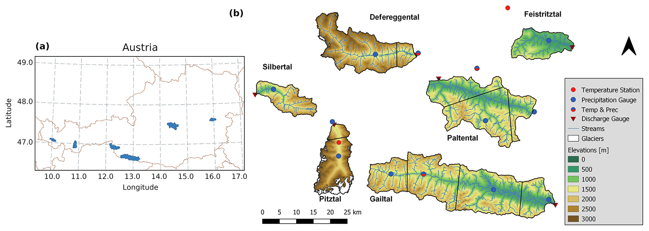
Figure 1 (a) Location of the catchments in Austria. (b) Catchment outlines indicating altitude, different precipitation zones, and the location and number of precipitation gauges and temperature stations (right) (Hanus et al., 2021).

Table 1 Catchment characteristics, land cover data and discharge regimes based on Mader et al. (1996), historical climate data (1985–2005) and average soil characteristics (0–2 m depth) derived from the SoilGrids250m 2.0 dataset (https://soilgrids.org/, last access: 20 March 2025).

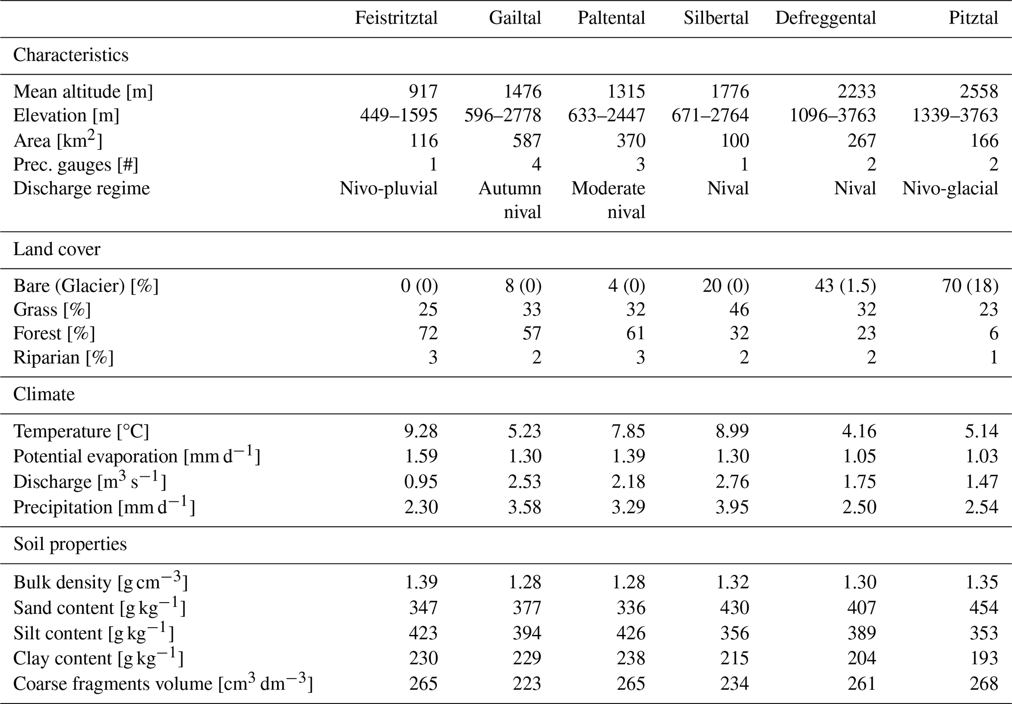
The Pitztal has the highest mean elevation (2558 m) and features a nivo-glacial discharge regime. This catchment is located in the west of Austria and is, due to its elevation, characterized by a large fraction of sparsely vegetated soils (70 %, with 18 % glacial coverage). The lowest-elevation catchment is the Feistritztal, with a mean elevation of 917 m. The Feistritztal is located in the eastern part of Austria, featuring a nivo-pluvial discharge regime and a relatively dense vegetation cover (72 % forest and 25 % grass). All other catchments, with mean elevations between 1315 m (Paltental) and 2233 m (Defreggental), exhibit a nival regime. The land cover varies in correspondence with elevation: high-altitude catchments are dominated by bare rock and grassland, while lower elevations are mainly forested. The Silbertal is the westernmost catchment, while the Feistritztal is the easternmost.

2.2 Data

This study provides a past–future analysis of modeled streamflow covering a period of 30 years: 1981–2010 and 2071–2100. The deployed datasets are elaborated on below.

2.2.1 Observational data (1981–2010)

Topographic information is derived from a 10 × 10 m digital elevation model (DEM) of Austria (https://www.data.gv.at/katalog/dataset/dgm, last access: 15 June 2021) and land cover data from the CORINE Land Cover dataset (https://land.copernicus.eu/pan-european-corine-land-cover, last access: 15 June 2021) (Table 1). Historic glacier outlines between 1997 and 2006 are available from the Austrian Glacier Inventory (https://www.uibk.ac.at/en/acinn/research/ice-and-climate/projects/austrian-glacier-inventory/, last access: 15 June 2021) (Lambrecht and Kuhn, 2007; Abermann et al., 2010). Glacial area changes are determined through linear interpolation on the observed outlines from 1997 to 2006 and subsequently extrapolated to estimate glacier areas up to 2015. Additionally, future glacier extents under various emission scenarios are available for the Pitztal from Zekollari et al. (2019), who simulated the future evolution of European glaciers using GloGEMflow. This model is an enhanced version of the Global Glacier Evolution Model by Huss and Hock (2015) that explicitly considers ice flow. The resulting future glacier extents under different emission scenarios are used in this study and are scaled to match extrapolated glacier areas in 2015.

2.2.2 Projected data (1981–2010 and 2071–2100)

For a meaningful comparison between past and future hydrological responses, we rely on climate model projections of precipitation and temperature. These projections are derived at the station scale for a historical (1981–2010) and future (2071–2100) period from 14 high-resolution regional climate models within the EURO-CORDEX ensemble (Table 2, Jacob et al., 2014). Precipitation and temperature data are provided on a daily basis at the station scale corresponding to the locations of precipitation and temperature stations (Fig. 1). Bias correction is applied using scaled distribution mapping, with a gamma distribution to remove systematic model errors (Switanek et al., 2017). For each regional climate model, we consider the two emission scenarios RCP4.5 and RCP8.5. RCP4.5 represents an intermediate pathway with partially reduced emissions, resulting in a radiative forcing of 4.5 W m⁻² by 2100. In contrast, RCP8.5 represents a trajectory characterized by increasing greenhouse gas emissions without mitigation measures.

Table 2 EURO-CORDEX projections used in this study (Jacob et al., 2014). Each ID represents a combination of a regional climate model (RCM) driven by a global climate model (GCM).

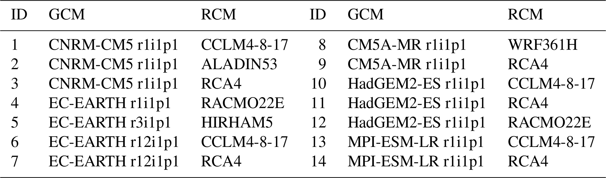
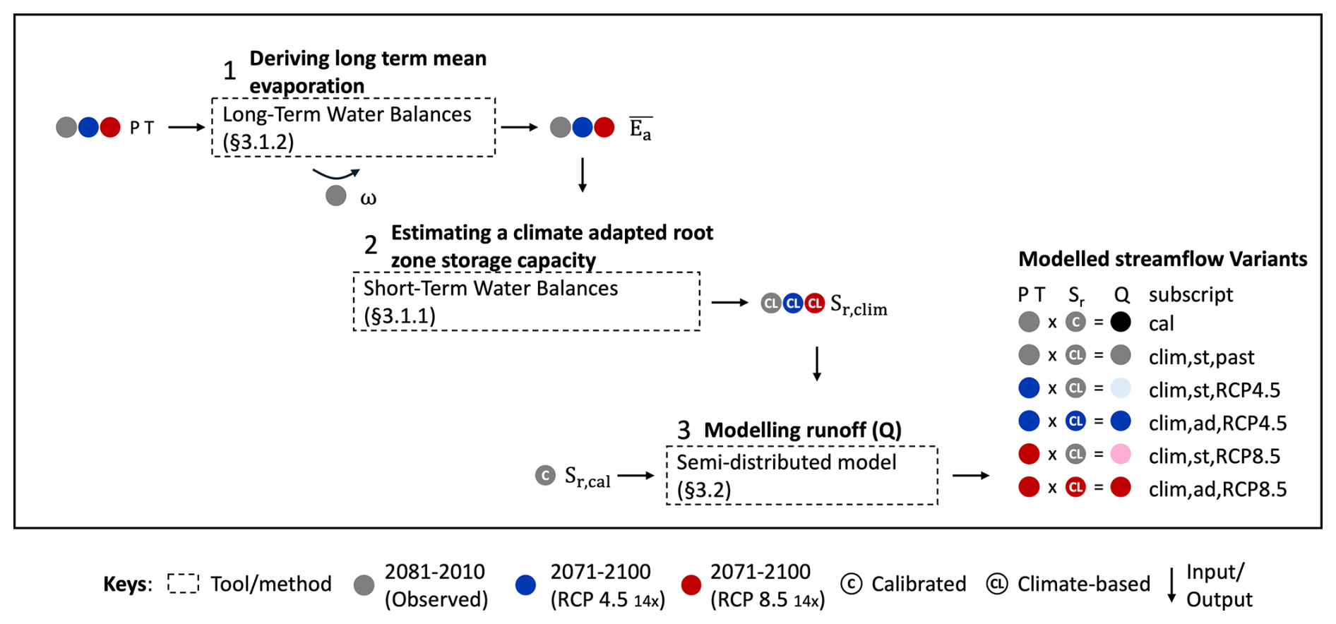
Figure 2 Process scheme of the adopted stepwise approach. The steps followed are as follows: estimate long-term runoff coefficient from the Budyko framework (3.1.2). Determine climate-based root zone storage capacity values (3.1.1). Implement calibrated S_r,cal and climate-based $S_{\mathrm{r},\mathrm{clim},\mathrm{past}}$ and $S_{\mathrm{r},\mathrm{clim},\mathrm{fut}}$ to model past and future streamflow, respectively (3.2). Numbering refers to the associated Methods sections. Abbreviations used include E_a for actual evaporation, P for precipitation, T for temperature, S_r,cal for the calibrated root zone storage capacity parameter and S_r,clim for the climate-based root zone storage capacity parameter. The subscript ad denotes parameters adapted to future climate, while st signifies parameters in stationary conditions.

3 Methods

This study adopts a top-down and process-based approach (Fig. 2), with the main aim to describe the impact of climate change on vegetation (Sect. 3.1) and the impacts thereof on streamflow in the past and future (Sect. 3.2). The study follows a five-step procedure: first, (1) the root zone storage capacity model parameters $S_{\mathrm{r},\mathrm{clim},\mathrm{past}}$ for the six study catchments are estimated from past water balance data (Sect. 3.1.1). Next, (2) future climate projections are combined with long-term water budget estimates following the Budyko hypothesis (Sect. 3.1.2) to estimate the corresponding future root zone storage capacities $S_{\mathrm{r},\mathrm{clim},\mathrm{fut}}$ (Sect. 3.1.3). Using a semi-distributed, process-based hydrological model, we then (3) compare $S_{\mathrm{r},\mathrm{clim},\mathrm{past}}$ to the corresponding values S_r,cal obtained by model calibration on past data and the associated model performances. Subsequently, we (4) apply $S_{\mathrm{r},\mathrm{clim},\mathrm{past}}$ together with future time series of P and T for RCP4.5 and RCP8.5 from an ensemble of 14 climate projections to quantify the effect of a changing climate on the hydrological response, assuming stationary catchment properties and thus time-invariant parameters (Sect. 3.2.2). On the condition that the model using the climate-based $S_{\mathrm{r},\mathrm{clim},\mathrm{past}}$ can reasonably describe past streamflow signatures, (5) we finally apply $S_{\mathrm{r},\mathrm{clim},\mathrm{fut}}$ with future climate projections to quantify the additional effects of non-stationary and thus time-variant root zone storage capacities on the hydrological response (Sect. 3.2.3).

3.1 Describing time-variant climate vegetation interactions

3.1.1 Using short-term water balances to quantify past root zone storage capacity

Previous studies have shown that different vegetation types develop root systems that can bridge droughts of varying return periods (Wang-Erlandsson et al., 2016). Following this assumption, the root zone storage capacity of riparian vegetation, grass and forest develops to endure droughts with a return period of, respectively, 2, 2 and 20 years. Corresponding root zone storage capacities for riparian vegetation ($S_{\mathrm{r},\mathrm{clim},\mathrm{rip}}$), grass ($S_{\mathrm{r},\mathrm{clim},\mathrm{grass}}$) and forest ($S_{\mathrm{r},\mathrm{clim},\mathrm{forest}}$) can then be estimated from the time series of maximum annual storage deficits $S_{\mathrm{r},\mathrm{D},\mathrm{yr}}$ using the Gumbel extreme value (GEV) distribution (e.g., de Boer-Euser et al., 2016; Nijzink et al., 2016). While the lower bound of the rooting depth is determined by the need to withstand moisture deficits associated with droughts of specific return periods, the upper bound is constrained by optimality principles – ensuring no excessive root development beyond what is necessary (Guswa, 2008).

The Memory method builds on this principle, describing how vegetation root zones adapt to prevailing climate conditions by creating a water buffer within reach of the roots, sufficient to bridge dry spells (Gentine et al., 2012; Donohue et al., 2012; Gao et al., 2014; van Oorschot et al., 2024a; van Oorschot et al., 2024b). We employ the Memory method to estimate the annual maximum excess of transpiration E_R over effective precipitation P_E. As a first approximation, this excess transpiration is assumed to originate from the water stored in the unsaturated zone. However, for various landscape types and vegetation species, roots may also directly tap groundwater (e.g., Fan et al., 2017). As input for the Memory method, we use a daily time series of effective precipitation P_E and transpiration E_R. Effective precipitation, defined as the liquid water input from snowmelt (M) plus rainfall after interception ($I=-\frac{\mathrm{d}{S}_{\mathrm{I}}\left(t\right)}{\mathrm{d}t}-E_I\left(t\right)$), is estimated from the water balance of the canopy storage (Eq. 1). As the interception storage capacity (I_max) of the interception storage (S_I) is unknown, a random sample of 300 a priori constrained I_max values is used (Supplement Fig. S2).

$$\begin{array}{}\text{(1)}& P_{\mathrm{E}}\left(t\right)=P\left(t\right)+M\left(t\right)-E_I\left(t\right)-{\displaystyle \frac{\mathrm{d}{S}_I\left(t\right)}{\mathrm{d}t}}\end{array}$$

The long-term mean transpiration (${\stackrel{\mathrm{‾}}{E}}_R$) is approximated by the long-term evaporation (${\stackrel{\mathrm{‾}}{E}}_A$) and derived from the long-term mean water balance (Eq. 2, all in mm yr⁻¹). This approximation operates under the assumption that long-term inter-catchment groundwater exchange and storage changes are negligible. The long-term mean transpiration is subsequently scaled to daily transpiration estimates using the daily difference between potential evaporation E_P and interception evaporation E_I (Eq. 3). By scaling E_R to E_P, we assume, overall, energy-limited conditions, as the snow-dominated Alpine catchments are characterized by early summer snowmelt and abundant summer rain that coincide with peak atmospheric water demand during the warm months.

$$\begin{array}{}\text{(2)}& {\displaystyle }{\stackrel{\mathrm{‾}}{E}}_R\approx {\stackrel{\mathrm{‾}}{P}}_E-\stackrel{\mathrm{‾}}{Q}\text{(3)}& {\displaystyle }{E}_R\left(t\right)=\left(E_{\mathrm{P}}\right(t)-E_I(t\left)\right)\cdot {\displaystyle \frac{{\stackrel{\mathrm{‾}}{E}}_R}{({\stackrel{\mathrm{‾}}{E}}_{\mathrm{P}}-{\stackrel{\mathrm{‾}}{E}}_I)}}\end{array}$$

Starting from daily deficits, we estimate the total water buffer stored in the root zone by accumulating over the total period of water shortage (T₀−T₁) (Eq. 4). Thereby, T₀ marks the first day at which transpiration exceeds effective precipitation ($(P_{\mathrm{E}}-E_R)<\mathrm{0}$), and T₁ represents the day at which the root zone storage deficit is restored to zero ($S_{\mathrm{r},\mathrm{D}}=\mathrm{0}$). The yearly maximum storage deficit $S_{\mathrm{r},\mathrm{D},\mathrm{yr}}$ is then selected and used as input for the GEV distribution to calculate S_r,clim for grass, forest and riparian vegetation. Note that because the derived estimates of $S_{\mathrm{r},\mathrm{clim},\mathrm{fut}}$ values represent root zone storages in catchments that are entirely covered by either forest, grass or riparian vegetation, these estimates may over- or underestimate the actual root zone storage capacity of a given catchment. Hence, the derived S_r,clim values are scaled to the respective areal fraction of each vegetation type. Due to the limited land coverage of riparian vegetation in each catchment, we will only discuss parameter changes and model results for forest and grass.

$$\begin{array}{}\text{(4)}& S_{\mathrm{r},\mathrm{D}}\left(t\right)=-min\underset{T_{\mathrm{0}}}{\overset{T_{\mathrm{1}}}{\int }}\left(P_{\mathrm{E}}\right(t)-E_R(t\left)\right)\end{array}$$

3.1.2 Long-term water balance framework for estimating changes in future runoff

While data for the historic time period are readily available, the long-term mean runoff for the future remains unknown and can be derived through the application of the Budyko framework. To estimate future evaporation under a changing climate, we here use (i) time series of projected future P together with (ii) estimates of future E_P based on projected T, combined with (iii) the long-term water balance, as described by the Budyko hypothesis (e.g., Turc, 1954; Mezentsev, 1955; Budyko, 1961; Fu, 1981; Zhang et al., 2004). The Budyko hypothesis describes how climate – expressed as the aridity index ($\frac{{\stackrel{\mathrm{‾}}{E}}_P}{\stackrel{\mathrm{‾}}{P}}$) – controls the long-term partitioning of precipitation ($\stackrel{\mathrm{‾}}{P}$) into evaporation ($\stackrel{\mathrm{‾}}{E_A}$) and streamflow ($\stackrel{\mathrm{‾}}{Q}$). The strong connection between evapotranspiration and runoff can be illustrated by the green-blue water paradox in the Alps, which indicates that rising temperatures increase evapotranspiration, ultimately leading to a decline in runoff (Mastrotheodoros et al., 2020). The Budyko space is defined by (i) the supply limit, as water can only evaporate based on availability, and (ii) the demand limit, as evaporation cannot exceed potential evaporation (Zhang et al., 2001; Xing et al., 2018; Mianabadi et al., 2020; Berghuijs et al., 2020 ). The Budyko curve broadly captures the partitioning of water fluxes in virtually every catchment worldwide, despite its simple structure and low requirement for input data (Berghuijs et al., 2020).

However, the original Budyko relationship does not explicitly consider the combined influence of soil, topography and vegetation, possibly explaining the systemic scatter found around the Budyko curve (Troch et al., 2013). As an attempt to overcome this limitation, parameterized Budyko equations, such as the Fu equation, account for bulk catchment biophysical features through the catchment-specific parameter (ω) (Eq. 5; Tixeront, 1964; Fu, 1981).

$$\begin{array}{}\text{(5)}& {\displaystyle \frac{{\stackrel{\mathrm{‾}}{E}}_A}{\stackrel{\mathrm{‾}}{P}}}=\mathrm{1}-{\displaystyle \frac{\stackrel{\mathrm{‾}}{Q}}{\stackrel{\mathrm{‾}}{P}}}=\mathrm{1}+{\displaystyle \frac{{\stackrel{\mathrm{‾}}{E}}_P}{\stackrel{\mathrm{‾}}{P}}}-(\mathrm{1}+({\displaystyle \frac{{\stackrel{\mathrm{‾}}{E}}_P}{\stackrel{\mathrm{‾}}{P}}}{)}^{\mathit{\omega }}{)}^{\frac{\mathrm{1}}{\mathit{\omega }}}\end{array}$$

Despite ongoing attempts (Jaramillo and Destouni, 2014; Van der Velde et al., 2014; Dwarakish and Ganasri, 2015; Jaramillo et al., 2018; Sankarasubramanian et al., 2020), the heterogeneity and interdependency of catchment-specific influences make it difficult to meaningfully disentangle the role of individual influencing factors for ω. Furthermore, when estimating changes in vegetation cover and adjustments in vegetation water use efficiency in response to fluctuating atmospheric CO₂ levels, large uncertainties arise (Yang et al., 2021). To minimize the impact of these uncertainties, we assume the relationship between evolving vegetation dynamics and changes in the catchment-specific parameter to be specific at the catchment scale. Furthermore, we assume that the general pattern of water partitioning described by the Budyko hypothesis – reflecting a past dynamic equilibrium – will remain largely unchanged under future conditions (Jaramillo et al., 2022). While ω is not strictly constant over time, several recent studies suggest that its variability due to climatic fluctuations is minimal in most regions worldwide (e.g., Ibrahim et al., 2025; Tempel et al., 2024; Wang et al., 2024). Thus, following Bouaziz et al. (2022), the explicit assumption here is that fixing ω is equivalent to keeping these other influencing factors constant, while increased E_A in more arid future conditions is sustained by increased root zone storage capacities (S_r). Hence, under the assumption of limited variability in ω under climate change, the ω_obs-parameterized Budyko curve, derived from past climate conditions, can be used for estimating future changes in long-term water flux partitioning and work towards a time-variant estimate of S_r,clim. Note that, while ω is strongly coupled with long-term mean water partitioning, this relationship is negligible over shorter timescales. This distinction justifies estimating long-term evaporative indices while accounting for evolving vegetation dynamics, without directly influencing short-term runoff dynamics. Here, the value of ω is estimated by solving Eq. (5) using observed climate and streamflow data, averaged over the historical 30-year study period (1981–2010; P_obs, T_obs, Q_obs). The resulting parameter value (ω_obs) hence reflects historical catchment conditions.

More specifically, future changes in climate are reflected in a shift in the aridity index AI, as a consequence of changes in precipitation rates ($\mathrm{\Delta }\stackrel{\mathrm{‾}}{P}={\stackrel{\mathrm{‾}}{P}}_{\mathrm{fut}}-{\stackrel{\mathrm{‾}}{P}}_{\mathrm{obs}}$), temperature and hence potential evapotranspiration ($\mathrm{\Delta }{\stackrel{\mathrm{‾}}{E}}_P={\stackrel{\mathrm{‾}}{E}}_{\mathrm{P},\mathrm{fut}}-{\stackrel{\mathrm{‾}}{E}}_{\mathrm{P},\mathrm{obs}}$) (Eq. 6; Fig. 3). These changes in climate cause a horizontal shift in the Budyko space, moving a catchment from its initial position (p_obs), along the ω_obs-parameterized Budyko curve, to a new position (p_fut). From the new long-term average, future evaporation and streamflow can be inferred from the evaporative index ($E_{A,\mathrm{fut}}/P_{\mathrm{fut}}$) and runoff ratio $\left(\frac{Q_{\mathrm{fut}}}{P_{\mathrm{fut}}}=\mathrm{1}-\frac{E_{A,\mathrm{fut}}}{P_{\mathrm{fut}}}\right)$, respectively (Eq. 7).

$$\begin{array}{}\text{(6)}& {\displaystyle }({\displaystyle \frac{{\stackrel{\mathrm{‾}}{E}}_P}{\stackrel{\mathrm{‾}}{P}}}{)}_{\mathrm{fut}}={\displaystyle \frac{{\stackrel{\mathrm{‾}}{E}}_{P,\mathrm{obs}}+\mathrm{\Delta }{\stackrel{\mathrm{‾}}{E}}_P}{{\stackrel{\mathrm{‾}}{P}}_{\mathrm{obs}}+\mathrm{\Delta }\stackrel{\mathrm{‾}}{P}}}\text{(7)}& {\displaystyle }({\displaystyle \frac{\stackrel{\mathrm{‾}}{Q}}{\stackrel{\mathrm{‾}}{P}}}{)}_{\mathrm{fut}}={\displaystyle \frac{{\stackrel{\mathrm{‾}}{Q}}_{\mathrm{obs}}+\mathrm{\Delta }\stackrel{\mathrm{‾}}{Q}}{{\stackrel{\mathrm{‾}}{P}}_{\mathrm{obs}}+\mathrm{\Delta }\stackrel{\mathrm{‾}}{P}}}=-({\displaystyle \frac{{\stackrel{\mathrm{‾}}{E}}_P}{\stackrel{\mathrm{‾}}{P}}}{)}_{\mathrm{fut}}+(\mathrm{1}+({\displaystyle \frac{{\stackrel{\mathrm{‾}}{E}}_P}{\stackrel{\mathrm{‾}}{P}}}{)}^{\mathit{\omega }}{)}^{\frac{\mathrm{1}}{\mathit{\omega }}}\end{array}$$

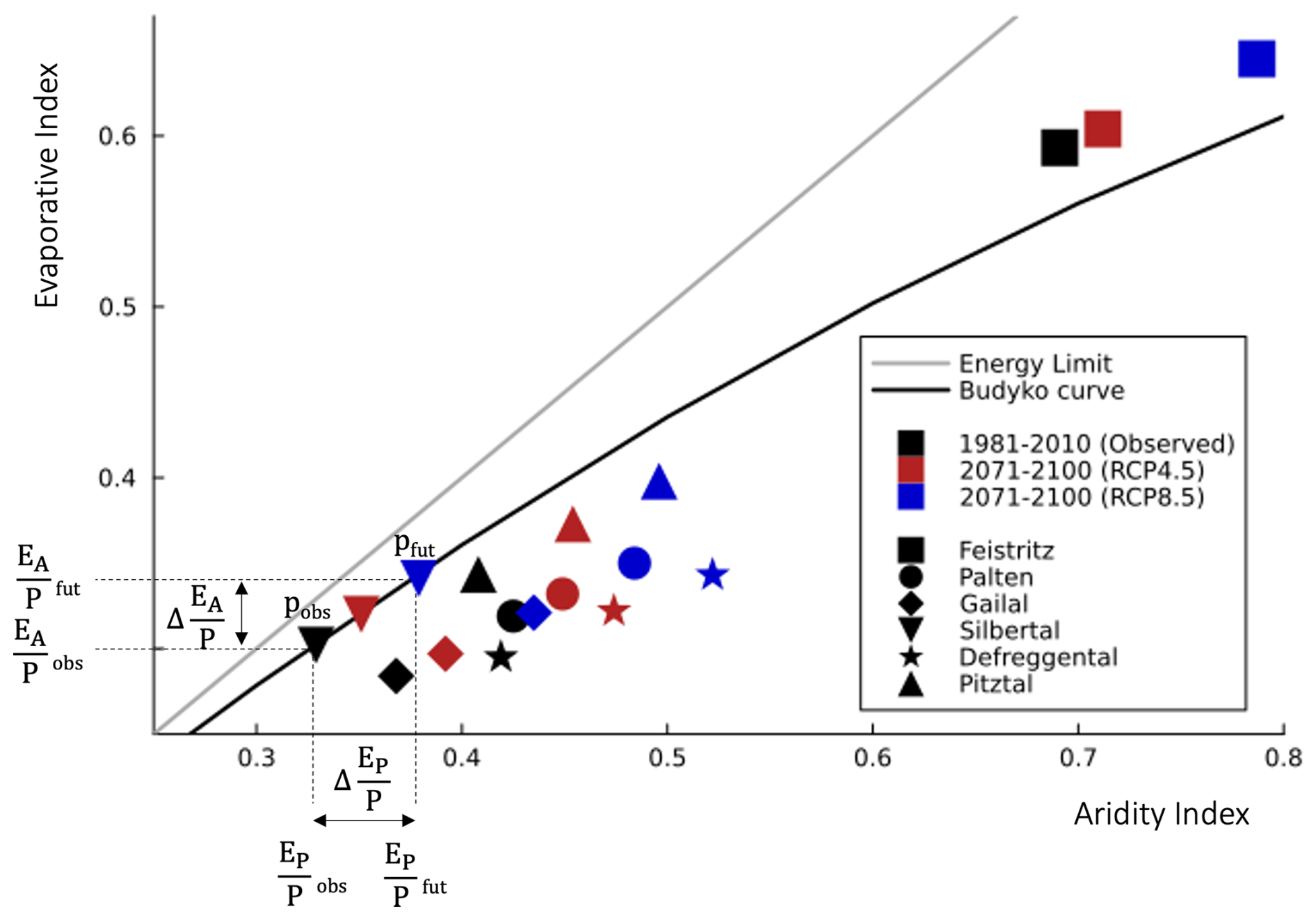
Figure 3 Representation of the Budyko space, showing the evaporative index $\frac{E_A}{P}$, the aridity index $\frac{E_{\mathrm{P}}}{P}$, and the energy and water limit. Using observed climate data, ${\frac{E_A}{P}}_{\mathrm{obs}}$ and ${\frac{E_{\mathrm{P}}}{P}}_{\mathrm{obs}}$, a catchment is plotted at position p_obs on the parametric Budyko curve with parameter ω_obs. Future climate change, and hence altered input data, results in an altered aridity index $\left({\frac{E_{\mathrm{P}}}{P}}_{\mathrm{fut}}\right)$, causing the catchment to move along the Budyko curve $\left(\mathrm{\Delta }\frac{E_{\mathrm{P}}}{P}\right)$ towards position p_fut that corresponds to a future evaporative index $\left({\frac{E_A}{P}}_{\mathrm{fut}}\right)$. Mean locations of the study catchments and their change over time are depicted in the Budyko space (average over 14 climate models is shown).

3.1.3 Estimating future root zone storage capacity $S_{\mathrm{r},\mathrm{clim},\mathrm{fut}}$

The combined use of predicted long-term water balance data and the Budyko framework allows us to estimate future root zone storage capacities $S_{\mathrm{r},\mathrm{clim},\mathrm{fut}}$. Using evaporative ratios from the Budyko framework, we approximate past and future long-term mean evaporation for different climate scenarios, i.e., the observed meteorological time series (1981–2010) and the 28 future climate projections (2071–2100, 14 RCMs × 2 RCPs), and we derive 29 long-term mean runoff coefficients (1-evaporative index). These long-term mean runoff coefficients complement the short-term water balance equation for the future. We, in turn, apply the Memory method (Sect. 3.1.1) for each of the climate scenarios, with varying return periods per vegetation type. Thereby, this approach results in one $S_{\mathrm{r},\mathrm{clim},\mathrm{past}}$ and 28 estimates of $S_{\mathrm{r},\mathrm{clim},\mathrm{fut}}$ for each vegetation type. Note that utilizing a range of 300 I_max values (Sect. 3.1.1) results in parameter ranges rather than single parameter values for S_r,clim.

To correct potential biases in projected climate data, $S_{\mathrm{r},\mathrm{clim},\mathrm{fut}}$ values are scaled to the difference between root zone storage parameters respectively obtained from observed and modeled past climate data, in line with Bouaziz et al. (2022) (Fig. S3).

3.2 Hydrological model

The influence of a climate-based, time-variant root zone storage capacity parameter on modeled streamflow is analyzed through a process-based, semi-distributed hydrological model (Prenner et al., 2018), as developed by Hanus et al. (2021), based on the approach proposed by Savenije (2010). This hydrological model represents the dominant rainfall-runoff processes in catchments based on topography and land cover classes. Thereby, the model accounts for the importance of landscape on runoff behavior, while retaining a simple model approach. More specifically, four parallel hydrological response units (HRUs) are represented by the model: bare rock, forested hillslope, grassland hillslope and riparian zone. Precipitation input is distributed across different HRUs and trickles down through various subsurface components, visualized by a bucket system. Water partitioning in the subsurface is governed by specific equations, each with several catchment-specific parameters that require calibration. All parameters remain constant across HRUs, except for the vegetation-dependent parameters: the interception storage capacity (I_max) and the root zone storage capacity (S_r,max). These storage capacity parameters vary among individual HRUs to account for differences in vegetation cover. The model schematic and relevant equations are provided in the Supplement (Fig. S1, Table S1), with a more detailed description available in Hanus et al. (2021).

3.2.1 Calibration and evaluation

In total, the model includes 20 parameters (including the parameter S_r,max) that are initially calibrated on observed streamflow data. For the Pitztal, an additional loss parameter is included that accounts for artificial water divergence through a pipe system from the catchment. Following the work of Hanus et al. (2021), all parameters are constrained a priori based on literature (Prenner et al., 2019; Gao et al., 2014). Additional constraints are provided to ensure that parameter combinations match the perceptions of the system, e.g., the interception capacity of forests must be greater than that of grass (Gharari et al., 2014).

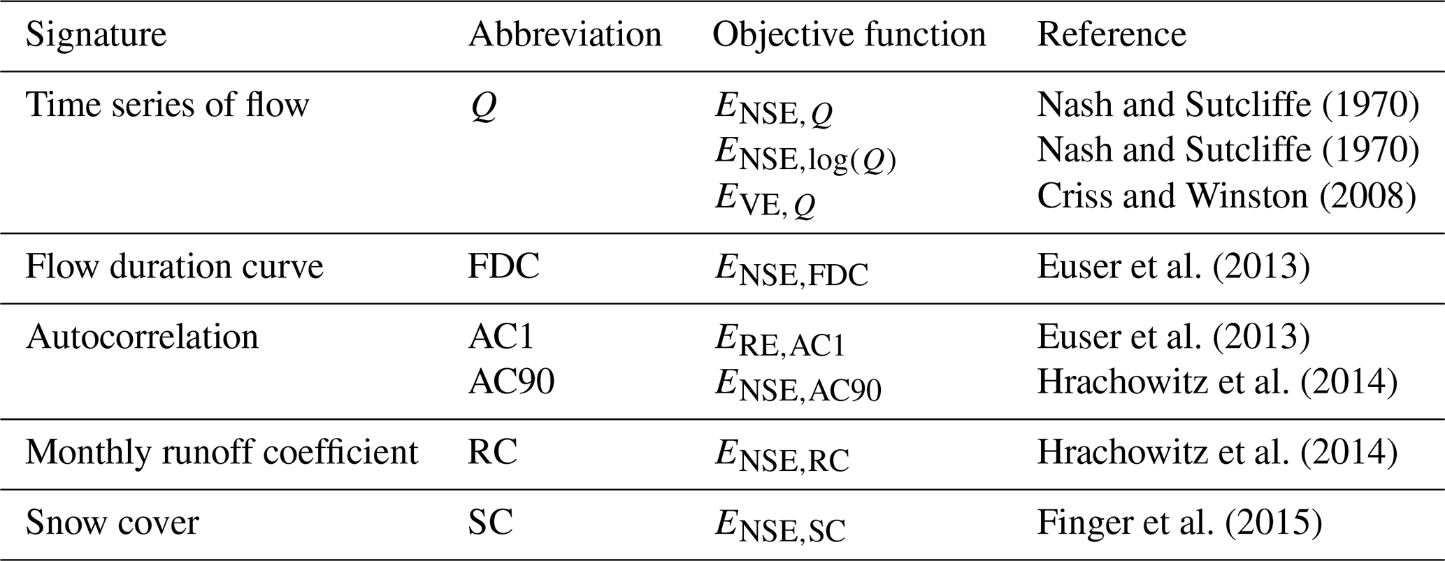
The model is then calibrated using eight objective functions (Table 3) to ensure adequate process representation and to reduce model uncertainties. This approach has proven effective in reducing false positives (e.g., Gupta et al., 2008; Efstratiadis and Koutsoyiannis, 2010; Hrachowitz et al., 2014) and mitigating the risk of “getting the right answers for the wrong reasons” (Kirchner, 2006). It thereby helps to distill meaningful signals in model parameters. The used objective functions include metrics to describe the magnitude and timing of high and low flows (Q, FDC), the memory of the catchment (AC1, AC90), the partitioning between evaporation and streamflow (RC), and the timing of snow cover (SC). All objective functions are equally weighted, as the calibrated model aims to represent the overall system dynamics. The overall model performance is then assessed by combining all individual objective functions using the Euclidian distance (E_D) from the perfect model fit, where a value of 1 indicates a perfect model (Eq. 8; Hulsman et al., 2021).

$$\begin{array}{}\text{(8)}& E_{\mathrm{D}}=\sqrt{{\displaystyle \frac{{\sum }_{n=\mathrm{1}}^N{\left(\mathrm{1}-E_N\right)}^{\mathrm{2}}}{N}}}\end{array}$$

Nash and Sutcliffe (1970)Nash and Sutcliffe (1970)Criss and Winston (2008)Euser et al. (2013)Euser et al. (2013)Hrachowitz et al. (2014)Hrachowitz et al. (2014)Finger et al. (2015)

Table 3 Objective functions used to calculate Euclidian distance (E_D) for calibration.

For each catchment, a Monte Carlo sampling strategy with 3 million realizations is performed, resulting in the same number of possible parameter combinations. These are subsequently referred to as “calibration parameter sets” (including the parameter S_r,cal). Based on a daily model time step, the calibration was performed over a 20-year period (October 1985–October 2005), with a prior 3-year model warm-up period. Only the best-performing 0.01 % of parameter sets, corresponding to a Euclidean distance E_D ≤0.2, are retained for further analysis to ensure a feasible computation time. Through this approach, ill-performing parameter combinations are excluded while still allowing the model a certain flexibility to account for parameter uncertainties.

The selected 300 parameter sets are subsequently evaluated over the post-calibration period (November 2005 to 2013 or 2015, depending on the catchment) using the objective functions outlined previously (Table 3).

3.2.2 Testing climate-based root zone storage $S_{\mathrm{r},\mathrm{clim},\mathrm{past}}$ for modeling past streamflow

To test the plausibility of root zone storage capacity estimates inferred from water balance data and to evaluate their influence on the model performance, we replace the calibrated values S_r,cal with the $S_{\mathrm{r},\mathrm{clim},\mathrm{past}}$ estimates. More specifically, the calibration parameters $S_{\mathrm{r},\mathrm{cal},\mathrm{forest}}$, $S_{\mathrm{r},\mathrm{cal},\mathrm{grass}}$ and $S_{\mathrm{r},\mathrm{cal},\mathrm{rip}}$ are replaced with a climate-based formulation, respectively $S_{\mathrm{r},\mathrm{clim},\mathrm{forest}}$, $S_{\mathrm{r},\mathrm{clim},\mathrm{grass}}$ and $S_{\mathrm{r},\mathrm{clim},\mathrm{rip}}$. Without any further re-calibration, the model is then re-run for the past period. This enables a comparison of the model's performance regarding the use of S_r,cal and S_r,clim, based on the eight hydrological signatures described above.

It is important to note that, due to the introduction of random I_max values in the water balance equation, a range is established for each S_r,clim. Hence, we randomly sample 10 values from each S_r,clim range. Therefore, the ensemble of 300 calibrated parameters for each vegetation class leads to 3000 climate-based equivalents for past conditions and for the two emission scenarios in the future. Hereafter, models using calibration and climate-based parameter sets are referred to with the subscripts cal and clim, respectively.

3.2.3 The effect of time-variant, future root zone capacity S_r,clim on streamflow

To investigate the influence of future adaptation of the root zone storage capacity on streamflow, we compare simulations using stationary $S_{\mathrm{r},\mathrm{clim},\mathrm{past}}$ and climate-adapted $S_{\mathrm{r},\mathrm{clim},\mathrm{fut}}$. For a comprehensive analysis, we first analyze the change between past and future streamflow, resulting from a changing climate, while keeping system parameters stationary, including the climate-based $S_{\mathrm{r},\mathrm{clim},\mathrm{past}}$. This run will hereafter be referred to as the stationary model run, using $S_{\mathrm{r},\mathrm{clim},\mathrm{stat}}$. Next, we quantify the additional effect of vegetation adaptation by modeling future streamflow using the climate-based, adapted $S_{\mathrm{r},\mathrm{clim},\mathrm{fut}}$. This run is hereafter referred to as the adapted model, using $S_{\mathrm{r},\mathrm{clim},\mathrm{adapt}}$. Both S_r,clim parameter sets are derived from the calibrated parameter sets, which are calibrated on past streamflow conditions. Without any further re-calibration, the S_r,cal parameter is exchanged for the $S_{\mathrm{r},\mathrm{clim},\mathrm{past}}$ and $S_{\mathrm{r},\mathrm{clim},\mathrm{fut}}$ parameters, respectively.

Next, hydrological change is assessed by examining various streamflow signatures over a 30-year period. These signatures correspond with those explored by Hanus et al. (2021), who delved into the effects of climate change between the past and future on identical study catchments. Nonetheless, our investigation predominantly focuses on evaluating the influence of vegetation adaptation on these streamflow signatures while only briefly discussing changes between past and future.

The streamflow characteristics include changes in mean annual discharge, indicating future water availability, mean monthly discharge, and both annual and seasonal runoff coefficients. Furthermore, changes in extreme hydrological events are analyzed according to Blöschl et al. (2017, 2019). Specifically, changes in the magnitude of high flows are assessed using time series of annual maximum flows (AMFs) and in the context of different return periods. Changes in timing are evaluated using the method of circular statistics (Young et al., 2000; Blöschl et al., 2017), which provides meaningful information about the timing of extreme events despite the turns of the year. However, this method cannot detect a bimodal flood season, as the average date of occurrence is located in the middle of the flood season. To address this possible non-detection, the relative frequency of AMFs occurring within 15 d is also studied. A 15 d time frame allows for the co-occurrence of different events while providing insight into relatively small changes in AMF over time.

Changes in low flows are assessed using a similar approach based on the annual minimum runoff over 7 consecutive days. Because low flows mainly occur in winter, a moving average from June to May is used to avoid complications with the turn of the year.

4 Results and discussion

4.1 Projected changes in climate

4.1.1 Hydroclimatic change

Annual median temperature and precipitation, averaged over 30 years, are projected to increase for the 2071–2100 period (Fig. 4). In spite of some variation between the 14 climate models (GCM–RCM combinations), similar temperature changes were found across all catchments, with multi-climate model median increases around 2–3 °C for RCP4.5 and 4–5 °C for RCP8.5 (vs. 1981–2010). The highest median increases are found in the Defreggental and Pitztal. Similarly, broadly consistent increases in precipitation are found across all catchments in the future. Increases are most pronounced for RCP8.5, where multi-climate model median changes range between +4 % in the Gailtal and +9 % in the Defreggental. However, the change direction depends on the climate model used, as projections range between −10 % and 20 % for RCP4.5, with spreads further increasing for RCP8.5.

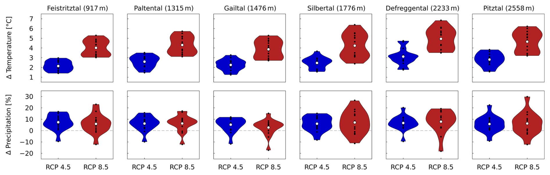
Figure 4 Violin plots displaying absolute changes in mean annual temperature and relative changes in mean annual precipitation for two RCPs and 14 climate models (black dots representing individual RCMs).

4.1.2 Future changes in the long-term water balance

For the 1981–2010 period, the Feistritztal and Silbertal show the highest and lowest aridity indices of, respectively, 0.69 and 0.23 (Fig. 3, Fig. S4, Table S2). This reflects the marked west-to-east gradient in hydroclimatic characteristics of the study catchments. Corresponding to the changes in aridity index, the evaporative index ranges between 0.28 in the Gailtal and 0.59 in the Feistritztal.

Catchment-specific values for ω range between 1.7 in the Defreggental and 3.0 in the Feistritztal, where higher values for ω (for a given aridity index) indicate more water use for evaporation. As such, differences in ω broadly reflect differences in land cover and, in particular, increases in forest cover along that gradient (Table 1, Table S2).

For the 2071–2100 period, aridity indices are projected to increase by roughly 0.03 in all catchments under RCP4.5 and up to twice as much under RCP8.5 (Fig. 3, Fig. S4, Table S2). This indicates drier future conditions with more energy available for evaporation. Again, the lowest and highest future aridity indices are found in the Silbertal (0.351–0.379) and Feistritztal (0.712–0.787), respectively.

Correspondingly, future evaporative indices are expected to increase by roughly 0.02 in all catchments for RCP4.5 and will range between 0.60 (Feistritztal) and 0.30 (Gailtal), with further increases for RCP8.5.

4.2 Water balance based on root zone storage capacity in the past and future

Using observed past data, the root zone storage capacity parameters range between $S_{\mathrm{r},\mathrm{clim},\mathrm{grass}}=$ 5–27 mm and $S_{\mathrm{r},\mathrm{clim},\mathrm{forest}}=$ 5–155 mm (Fig. 5). Regardless of the vegetation type, the lowest and highest S_r,clim values are found in the Pitztal and the Feistritztal, respectively. The low root zone values in the Pitztal suggest shallow hydrologically active soil depths, which is realistic given that bare rock covers 70 % of the catchment area. Consequently, the storage capacity is largely controlled by $S_{\mathrm{R},\mathrm{bare},\mathrm{cal}}$, which is determined through calibration and a priori constrained. This constraint reflects the substrate’s limiting effect on rooting depth and, in turn, the lower storage capacity in this catchment. Conversely, the highest values are found in the Feistritztal, where 72 % of the area is forested. This relationship between vegetation cover and root zone storage capacity is consistent with findings by Merz and Blöschl (2004) in a model calibration experiment for 308 catchments in Austria. Note that, unlike S_R,cal, S_R,clim is not constrained a priori but is instead determined by optimality principles, energy limitations and the areal fraction of vegetation.

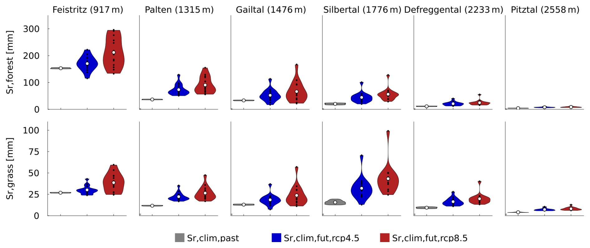
Figure 5 Estimates for $S_{\mathrm{r},\mathrm{clim},\mathrm{past}}$ and $S_{\mathrm{r},\mathrm{clim},\mathrm{fut}}$ for forest (upper row) and grassland (lower row) landscape elements, inferred from observed past and corrected projected future climate data using the Memory method. A similar figure including calibrated parameter values (S_r,cal) is included in the Supplement (Fig. S5).

The spread in $S_{\mathrm{r},\mathrm{clim},\mathrm{past}}$ is below 5 mm in all catchments for all vegetation types and directly results from the 300 different interception capacities (I_max) applied in the Memory method.

For the 2071–2100 period, moisture deficits in the root zone are projected to increase as a result of increased dryness indices and the associated higher evapotranspiration rates (Eqs. 3 and4, Fig. 3). While $S_{\mathrm{r},\mathrm{clim},\mathrm{forest}}$ remains largely stable in the Pitztal, it increases in the remaining catchments by at least 10 mm (100 %, Defreggental) and by up to 30 mm (75 %, Feistritztal) under RCP4.5, with further increases for RCP8.5.

Similarly, $S_{\mathrm{r},\mathrm{clim},\mathrm{grass}}$ increases by 4–20 mm for RCP4.5 (6–32 mm, RCP8.5) in all catchments in the future. This translates into relative changes in $S_{\mathrm{r},\mathrm{clim},\mathrm{grass}}$ of 14 %–125 %, with the lowest increases in the Feistritztal and the Pitztal. The largest increase in $S_{\mathrm{r},\mathrm{clim},\mathrm{grass}}$ is found in the Silbertal.

The spread in estimated S_r,clim values increases for the future period for all vegetation types (most outspoken for RCP8.5), thereby reflecting the uncertainty in the 14 climate models. The spread in $S_{\mathrm{r},\mathrm{clim},\mathrm{past}}$ ranges between 5–10 mm for forest and 2–8 mm for grass, with the largest spread found in the Silbertal. For $S_{\mathrm{r},\mathrm{clim},\mathrm{forest}}$ and $S_{\mathrm{r},\mathrm{clim},\mathrm{grass}}$, the spread is even more pronounced, ranging between 30–110 mm (45–160 mm, RCP8.5) and 18–60 mm (28–36 mm, RCP8.5), respectively. Notwithstanding these uncertainties, the spread in S_r,clim is much smaller compared to the spread in S_r,cal arising from calibration (Fig. S5).

4.3 Modeled hydrological response

Root zone storage capacity parameters, respectively obtained through calibration (S_r,cal) and the Memory method ($S_{\mathrm{r},\mathrm{clim},\mathrm{past}}$), are subsequently implemented in the hydrological model.

4.3.1 Calibration and evaluation

Both models, respectively using the calibrated (S_r,cal) and water balance-based ($S_{\mathrm{r},\mathrm{clim},\mathrm{past}}$) estimates of the root zone storage capacity parameter, broadly reproduce the main features of the observed hydrological response in all study catchments. Using the calibrated parameters, the overall model performance ranges between $D_{\mathrm{E},\mathrm{cal},\mathrm{tot}}$ = 0.81–0.88 and $D_{\mathrm{E},\mathrm{clim},\mathrm{tot}}=$ 0.80–0.87 during the calibration period and remains stable for the evaluation period, with $D_{\mathrm{E},\mathrm{cal},\mathrm{tot}}=$ 0.78–0.89 and $D_{\mathrm{E},\mathrm{clim},\mathrm{tot}}=$ 0.80–0.85 (Fig. S6). Hence, differences in the performance of the two model implementations are limited (Fig. 6), with a maximum difference $\mathrm{\Delta }{D}_{\mathrm{E},\mathrm{tot}}=$ −0.06 for calibration and −0.07 for evaluation, respectively.

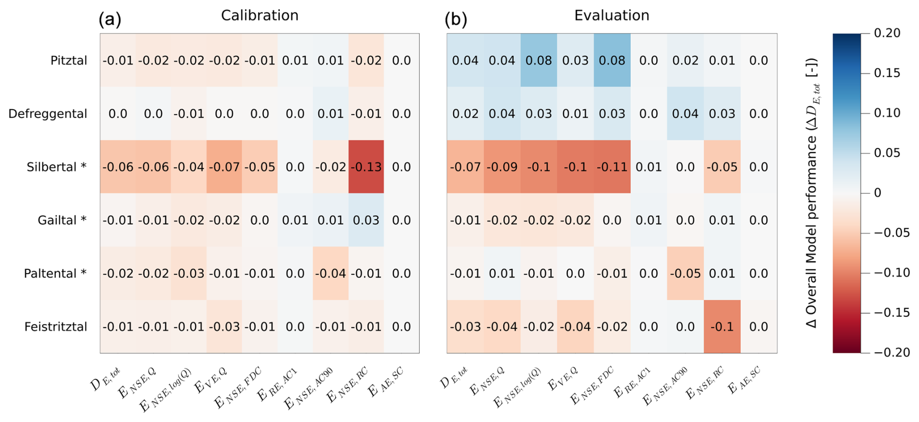
Figure 6 Difference in model performance between the calibrated and climate-based models during the calibration (a) and evaluation (b) period for the overall model fit ($\mathrm{\Delta }{D}_{\mathrm{E},\mathrm{tot}}=D_{\mathrm{E},\mathrm{clim},\mathrm{tot}}-D_{\mathrm{E},\mathrm{cal},\mathrm{tot}}$) and eight objective functions. Negative values indicate a better model performance of the calibrated model and vice versa. Catchments marked with an asterisk (^*) use an 8-year evaluation period instead of 10 years (Sect. 3.2.1). Table 3 provides a description of the objective functions.

Accordingly, the modeled hydrographs indicate that the short-term flow dynamics (Figs. 6, S7–S11) and mean regime curves (Fig. 7) are, in general, adequately captured by the models, regardless of the parameter set used. In some cases, the modeled short-term peak flows remain underestimated (e.g., in the Paltental and Defreggental). This underestimation is likely associated with uncertainties in precipitation observations in very localized high-intensity convective rainfall events (Hrachowitz and Weiler, 2011). Compared to the other catchments, the Pitztal shows a higher model spread. This likely stems from glacier presence, introducing an additional model parameter, and the extensive bare areas with limited storage capacity and hence higher climatic sensitivity.

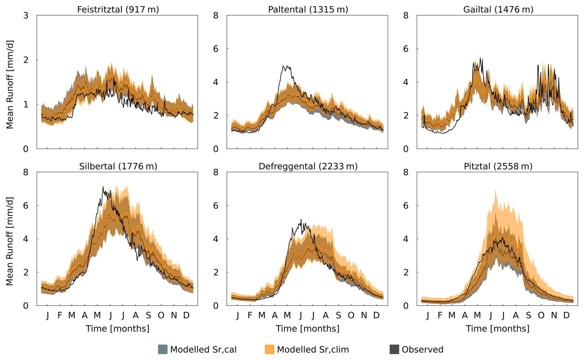
Figure 7 Annual mean regime curves for the six study catchments over the 1981–2010 period. Solid lines represent mean runoff, and shaded bands indicate ±1 SD.

Hence, we conclude that both the calibrated and climate-based models adequately reproduce the general magnitudes and seasonality in all catchments. The overall good model performance implies that the retained climate-based parameter sets can be used for modeling future streamflow.

4.4 Future streamflow projections

Future streamflow for the 2071–2100 period is estimated by forcing the hydrological model with the projected climate data. To test the impact of a dynamical evolution of the root zone storage capacity on the modeled hydrological response, the modeled streamflow from a model run with stationary $S_{\mathrm{r},\mathrm{clim},\mathrm{stat}}$ parameters, obtained from past predicted water balance data, is compared to a model run with an adapted formulation of the $S_{\mathrm{r},\mathrm{clim},\mathrm{adapt}}$ parameters (Fig. 8), based on projected future water balance data. The two model runs are hereafter referred to as the stationary and adapted models.

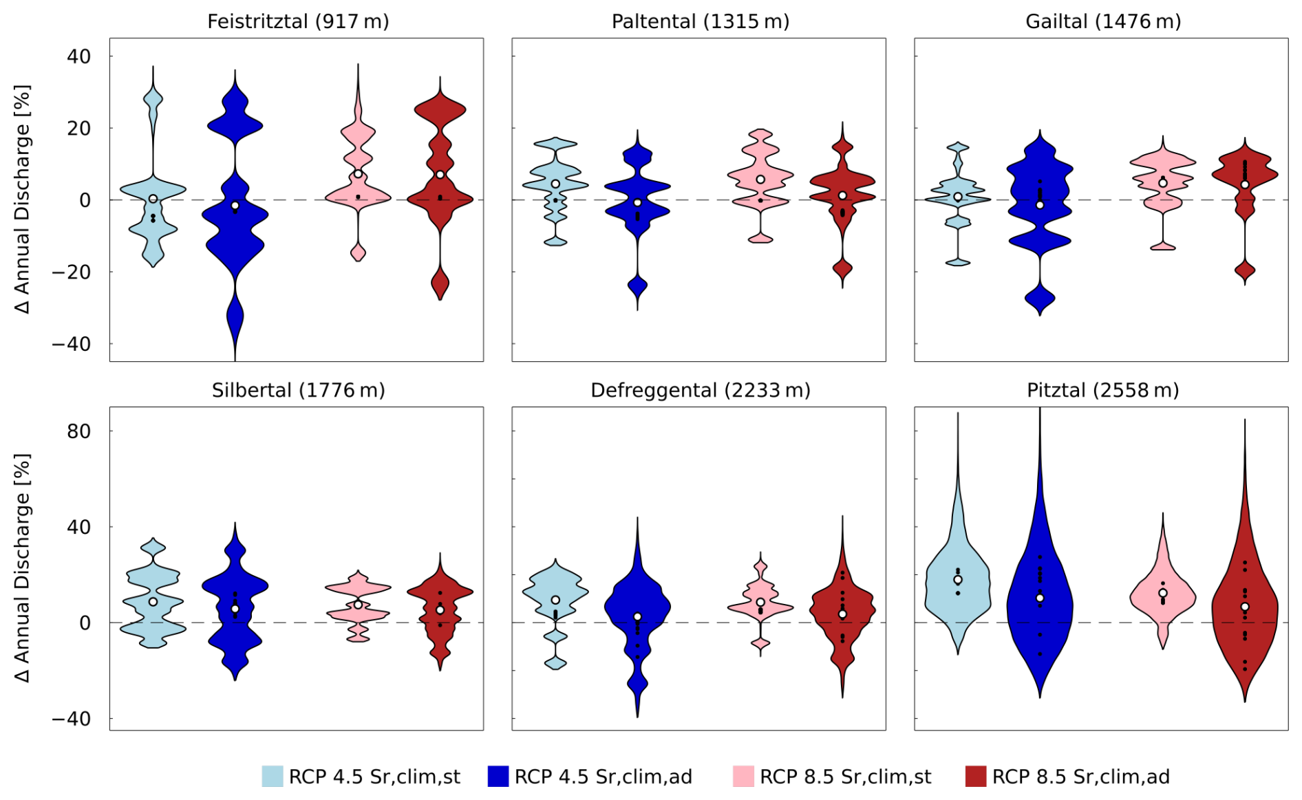
Figure 8 Relative changes in mean annual streamflow for all catchments, using models featuring $S_{\mathrm{r},\mathrm{clim},\mathrm{stat}}$ and $S_{\mathrm{r},\mathrm{clim},\mathrm{adapt}}$, for two RCPs and 14 climate models (black dots representing individual RCMs).

4.4.1 Annual discharges

In general, mean annual streamflow in the study catchments exhibits only modest sensitivity to changing climatic conditions (Figs. 8, S12). The magnitude and direction of the change in streamflow differ per catchment and climate projection used and result from the combined influence of the projected increased annual precipitation and increased evaporation (Fig. 3, Fig. S4, Table S2). The multi-climate model median temporal change in streamflow across all climate projections varies from −4 % (Feistritztal) to +10 % (Pitztal) for RCP4.5, while differences are slightly more pronounced for RCP8.5. Differences in the median modeled temporal change in streamflow between the stationary and adapted models are very minor, which is in line with the findings of Bouaziz et al. (2022).

The modeled mean annual streamflow estimates are also characterized by a relatively high spread (> 100 %) for both model runs and both climate scenarios, arising from the uncertainty in the projected hydroclimatic variables from the 14 climate models. Overall, and due to the additional uncertainty introduced by the estimation of $S_{\mathrm{r},\mathrm{clim},\mathrm{fut}}$, the spread in modeled changes in annual streamflow is somewhat more pronounced for the adapted model, with a spread up to ∼ 120 % for the Pitztal.

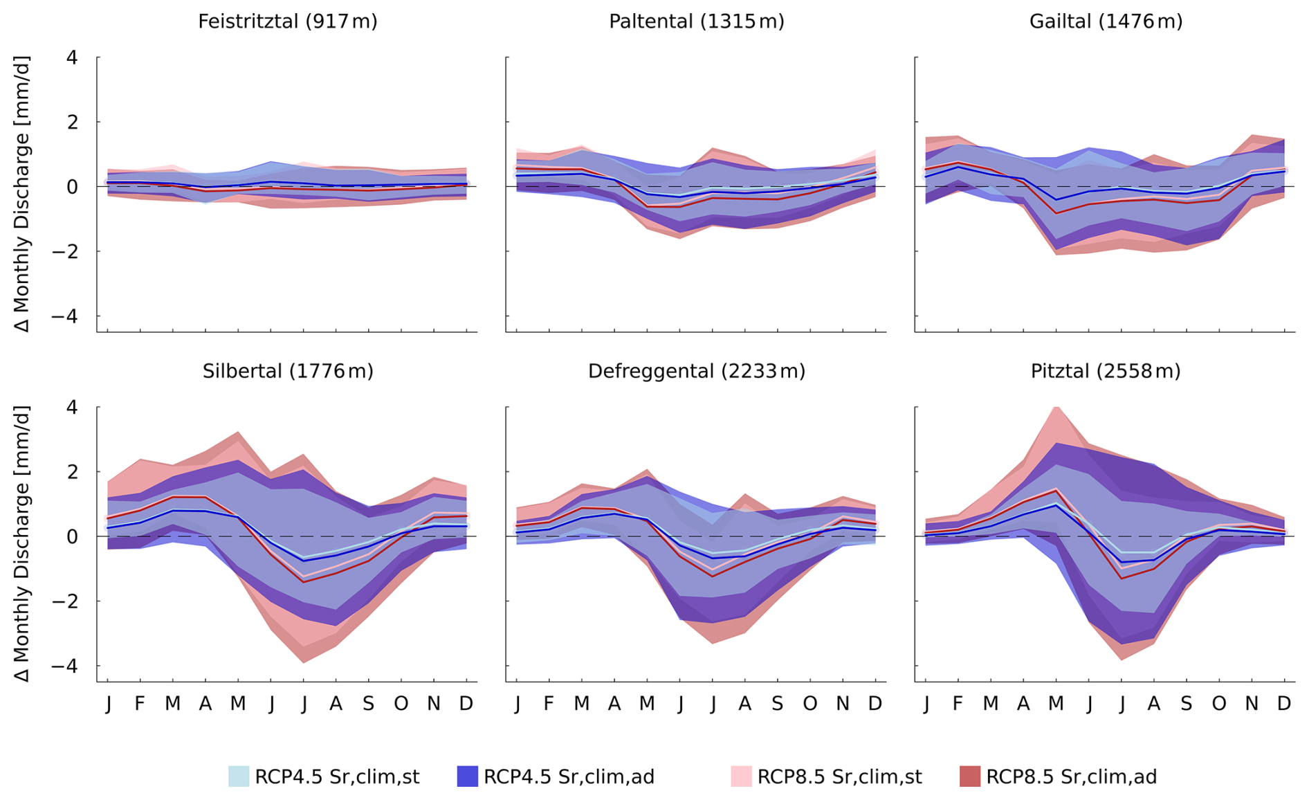
Figure 9 Absolute changes in mean monthly streamflow, using data between the 1981–2010 period and the 2071–2100 period for two RCPs and 14 climate models. Solid lines represent mean runoff, and shaded bands indicate ±1 SD.

4.4.2 Monthly discharges

The stationary and adapted runs predict consistent seasonal streamflow changes across catchments, varying in magnitude (Fig. 9). Winter and early spring flows may rise by up to ∼ 1 mm d⁻¹ (90 %) under RCP4.5 and ∼ 1.5 mm d⁻¹ under RCP8.5, while summer and early autumn flows could drop by ∼ 1 mm d⁻¹ (20 %) for RCP4.5 and ∼ 1.5 mm d⁻¹ for RCP8.5. The Feistritztal is an exception, showing little change in monthly streamflow. The only notable difference between the stationary and adapted models is for mid-summer flow in high-elevation catchments, projected by the adapted model to be up to ∼ 0.5 mm d⁻¹ (Pitztal) lower than the stationary model.

No significant difference in change timing is found between the stationary and adapted models. Both show the highest flow increases from February (Gailtal) to May (Pitztal) and the greatest flow reductions from May (Gailtal) to July at high elevations. This shift towards earlier peak flows reflects earlier onset of the melting season in a warmer climate. In lower catchments (Feistritztal, Paltental), the shifts in timing are less distinct.

The spread in results is found to be slightly larger for the adapted model and originates from the climate-model-induced spread in $S_{\mathrm{r},\mathrm{clim},\mathrm{fut}}$. In the stationary model, the absolute model spread reaches up to ∼2 mm d⁻¹ (Pitztal) for RCP4.5 and more for RCP8.5, while for the adapted model, the spread is around ∼ 3 mm d⁻¹, with further increases under RCP8.5).

4.4.3 Runoff coefficient

Both models indicate stable median runoff coefficients (C_R) at low elevations under RCP4.5 and 8.5. At higher elevations, the stationary model predicts C_R increases by up to ∼0.05 for RCP4.5 and ∼0.20 for RCP8.5, with the adapted model projecting slightly but systematically lower increases (∼0.05) than the stationary model (Fig. 10). This supports the findings of Bouaziz et al. (2022), who also reported systematically lower increases in runoff coefficients using a similar adapted model in the Meuse river basin (France, Belgium). This pattern illustrates the green-blue water paradox, where increased root zone storage capacity ($S_{\mathrm{r},\mathrm{clim},\mathrm{fut}}$) in the adapted model enhances subsurface water availability for vegetation. As a result, more water is allocated to transpiration (green water), reducing its contribution to streamflow (blue water). This mechanism is further supported by the observation that for both RCP4.5 and RCP8.5, the largest difference between adapted and stationary model projections of ΔC_R is found in the Paltental, which is also the catchment with the largest relative change in S_r,clim between past and future. Although the two hydrological model runs provide largely consistent results, the direction of change in the annual runoff coefficient C_R is highly dependent on the climate projection used (Fig. 10).

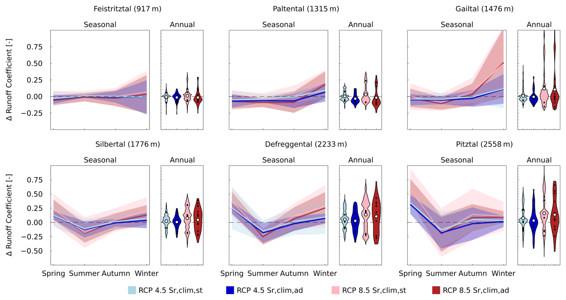
Figure 10 Absolute changes in 30-year average seasonal runoff coefficients for two RCPs and 14 climate models (black dots representing individual RCMs) using the climate-based stationary and adapted models.

The stationary and adapted hydrological models also project similar changes in seasonal runoff coefficients. In correspondence with changes in monthly discharge, seasonal runoff coefficients increase in the winter and spring with up to ΔC_R∼0.32 and decrease in the summer months with up to ΔC_R∼0.15 as a result of changes in snowmelt contributions (see Fig. 10). Slight differences exist between the stationary and adapted model runs in the Paltental and Pitztal, with the latter projecting autumn ΔC_R increases that are around 0.1 lower than those for the stationary model. For most study catchments, and irrespective of the model run, changes in the seasonal runoff coefficient become more pronounced for RCP8.5, as temperatures and consequently late-winter and early-spring snowmelt further increase. A similar pattern is found for relative changes in the runoff coefficients (Fig. S14).

4.4.4 Annual maxima (timing and magnitude)

According to both the stationary and adapted model runs, the timing of annual maximum flows (AMFs) will experience future shifts of up to several weeks (Fig. 11, Table S3). While at higher elevations, future AMF is projected to occur ∼ 1–3 weeks earlier under RCP4.5, the low-lying Gailtal will experience future AMF, on average, 3 weeks later, towards the end of October (Figs. 11; 12, right). The earlier AMF at high elevations is a result of earlier snowmelt; the later occurrence of AMF in the Gailtal, in contrast, is governed by a higher proportion of autumn precipitation falling as rain instead of snow (Vormoor et al., 2015; Brunner et al., 2020; Hanus et al., 2021). For RCP8.5, the shifts are more pronounced, by ∼ 1–2 weeks.

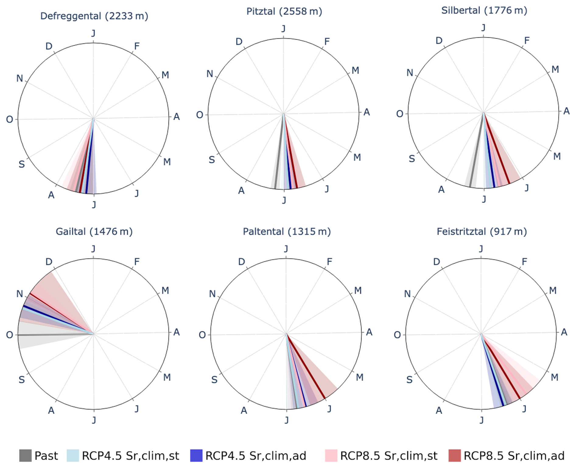
Figure 11 Simulation of the mean occurrence of the average timing of annual maximum flow over 30 years for two RCPs and 14 climate models using the climate-based stationary and adapted models. Uncertainty bands of ±1 SD are shaded, and lines connecting 15 d periods are used to allow for better visualization.

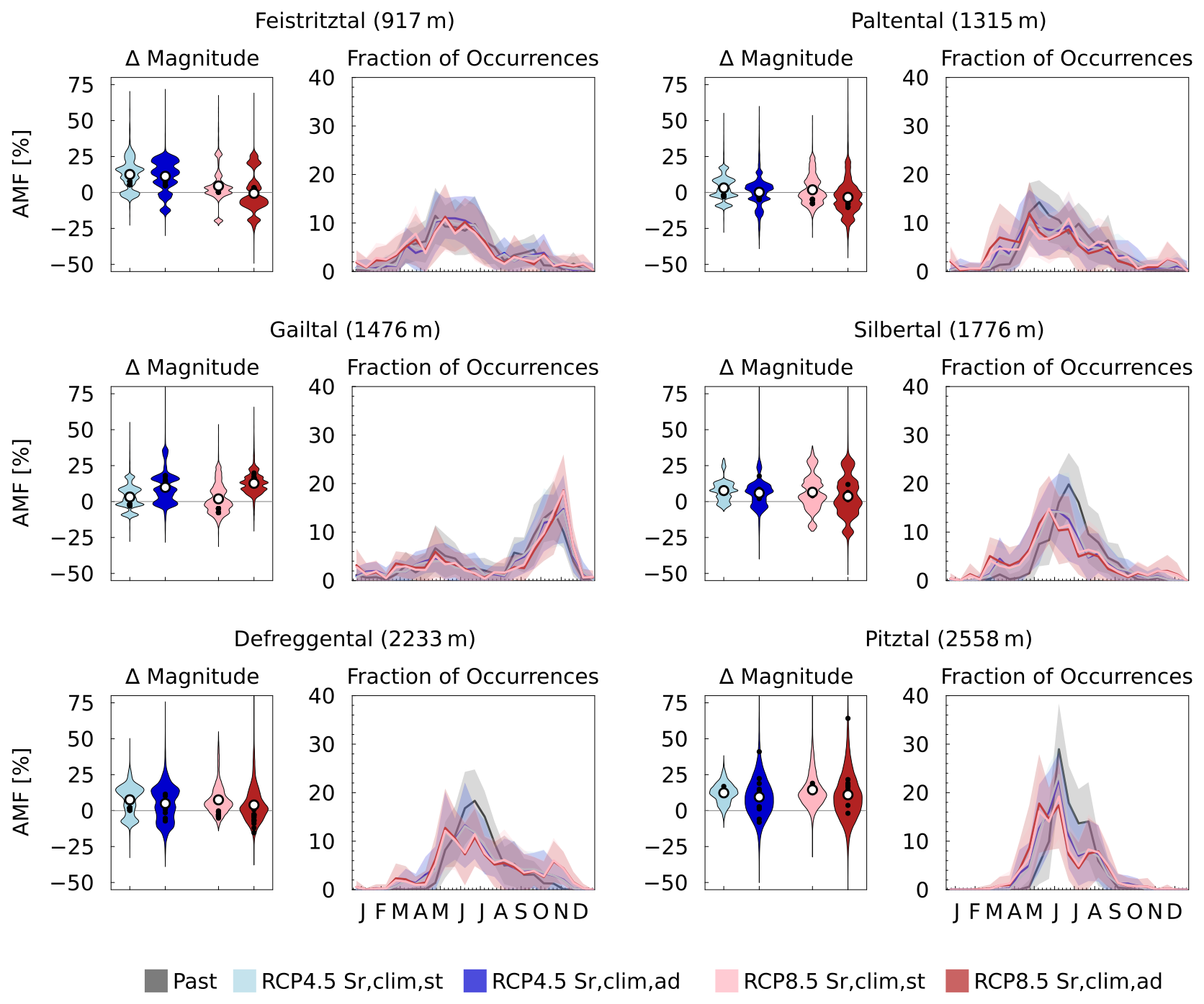
Figure 12 For each catchment: (left) relative change in the 30-year average magnitude of annual maximum flow (AMF). (Right) Mean fraction of occurrences of AMFs over 30 years, utilizing a 15 d time window. Uncertainty bands of ±1 SD are shaded, and lines connecting 15 d periods enhance visualization. Both magnitude and timing are assessed for two RCPs and 14 climate models (black dots representing individual RCMs), employing both climate-based stationary and adapted models.

Overall, the adapted model projects slightly stronger shifts in timing than the stationary model. For RCP4.5, the shifts extend over an additional 2–3 d, which increases up to 8 d for RCP8.5. One exception is the Paltental, where the shifts in AMF timing for the adapted model are between 6 d (RCP4.5) and 17 d (RCP8.5) more pronounced compared to the stationary model.

A bimodal AMF seasonality is observed in the past for the Gailtal (Fig. 12, right), with peaks in May and September, characteristic of the autumn-nival flow regime (Mader et al., 1996; Blöschl et al., 2011). This pattern is expected to persist, while higher-elevation catchments, especially under RCP8.5, may transition to a bimodal AMF with peaks in early May and mid-June (Fig. 11). This finding suggests a future extension of the length of the flood seasons in essentially all study catchments, ranging from 1 month in the Paltental to 2–3 months in the Silbertal and Defreggental, regardless of the model run.

Both models project similar future AMF changes in direction and magnitude. AMF may increase by up to ∼ 10 % under RCP4.5, with the lowest rise (∼ 5 %) in the Paltental, potentially due to reduced late-spring snowmelt offsetting increased precipitation. RCP8.5 shows smaller changes in AMF magnitude, due to less snowmelt and higher evaporation under higher temperatures, both increasing soil storage deficits and hence lowering runoff. The adapted model projects on average ∼ 5 % lower AMF increases, which is linked to the higher root zone storage capacity, reducing runoff during extremes. Only in the Gailtal, the adapted model predicts ∼ 15 % larger changes. Both the stationary and adapted models indicate a consistent increase in absolute AMF magnitude with higher return periods across all catchments (Fig. S15).

4.4.5 Annual minima (timing and magnitude)

The maximum fraction of occurrences of 7 d consecutive low flows increases with altitude and ranges between 17 % (Feistritztal) and 47 % (Gailtal, Fig. 13, right). The peak in low flow occurs between February in lower-elevation catchments (Feistritztal) and March for higher-elevation catchments (Pitztal).

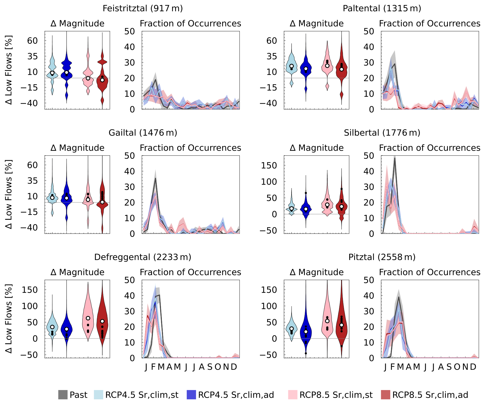
Figure 13 For each catchment: (left) relative change in the 30-year average magnitude of 7 d consecutive lowest flows. Note the different scales for high- and low-elevation catchments. (Right) Mean fraction of occurrences of yearly lowest 7 d consecutive flow in 30 years, using a 15 d time window. Uncertainty bands of ±1 SD are shaded, and lines connecting 15 d periods enhance visualization. Both magnitude and timing are assessed for two RCPs and 14 climate models (black dots representing individual RCMs), employing both climate-based stationary and adapted models.

Both models project similar future changes in low flow timing, magnitude and spread. Winter low flow occurrences are expected to decline, especially under RCP8.5, with reductions of ∼ 10 %, reaching ∼ 20 % in the Paltental and Silbertal. This aligns with Bouaziz et al. (2022), who found no significant differences in 7 d low flow probabilities between models in the Meuse basin.

Low flow occurrences become more evenly distributed throughout the year, with the least seasonality in the Feistritztal. At higher elevations, low flows shift earlier, extending the period of substantial low flows. Previously peaking in February to March, future low flows are expected from January to March due to earlier onset of the snowmelt season. At lower elevations, autumn low flows are projected to increase, with a maximum increase of 13 % in the Paltental, due to higher storage deficits under reduced precipitation and higher temperatures.

A broadly similar increase in future annual low flow magnitudes is projected by the stationary and adapted models, with a consistent increase in the magnitude of median low flows (Fig. 13, left). In high-elevation catchments, this increase is more pronounced for RCP8.5 and reaches an increase by up to 60 % (Defreggental). Although the adapted projections show a high resemblance to the stationary model, change projections are on average 1 %–5 % lower for RCP4.5 and 4 %–15 % for RCP8.5. Hence, the adapted model projects a smaller magnitude of future low flows, which is related to increased values of the climate-based adapted root zone storage capacity parameters and related higher water retention in the root zone, resulting, in turn, in reduced runoff volumes.

The direction of change is very uncertain for low flows in the Feistritztal, Paltental and Gailtal. While for the stationary model, projected spreads in magnitude of low flows vary between 80 % (Paltental) and 240 % (Pitztal), the adapted results in a larger spread, between 110 % and 240 %, respectively (for RCP8.5).

5 Broader implications and outlook

A broad consistency was found when modeling streamflow with either a stationary or an adapted root zone storage capacity parameter. While projections show significant changes in the future root zone storage capacity of forests and grasslands, with potential increases of up to 100 % and 45 %, respectively, compared to historical levels, accounting for this by adjusting the associated model parameters results in only a limited decrease in projected streamflow and differences in annual mean streamflow projections that are close to zero. This also holds for differences in 7 d consecutive low flows and fractions of occurrences of high and low flows, for which differences are very limited for all catchments. Differences in the annual runoff coefficient and annual maximum flows projected by the stationary and adapted model runs are around 5 %. However, on a seasonal scale, the model differences can be larger, with the adapted model projecting up to −10 % lower monthly discharges and seasonal runoff coefficients. In general, in our study, the differences between the model projections are the smallest for the lower-elevation catchments and increase with elevation. This pattern corresponds to the projected magnitude of change between past and future streamflow, which is particularly pronounced in higher-elevation catchments.

Our findings point to the same direction of change as previous studies that implemented vegetation dynamics in hydrological models, although our modeled changes are generally smaller. Bouaziz et al. (2022) modeled changes in annual mean (−7 %), annual maximum (−5 %) and 7 d low (0 %) flows when replacing calibrated, stationary root zone storage capacity parameters with adapted estimates. Merz et al. (2011) also showed that models with stationary parameters overestimate median average annual and maximum streamflow by +15 % and +35 %, respectively. Similarly, Duethmann et al. (2020) and Speich et al. (2018) showed model overestimation to reduce when accounting for evolving vegetation dynamics. In response to changes in vegetation, evaporation rates were found to increase from +4 % (Bouaziz et al., 2022) to as high as +67 % (Merz et al., 2011), indicating substantial variability on the order of magnitude of future changes to occur in adapted modeling. Although the magnitude of change in our study is less pronounced, a similar direction of change is distinguished: runoff coefficients are found to decrease, implying higher evaporation rates.

The six studied catchments are all relatively humid (Fig. 3) and are therefore characterized by shallow hydrologically active root zones (Merz and Blöschl, 2004). Also, the effects of rising precipitation and higher temperatures typically balance each other, thereby limiting the potential for significant expansion in root zone storage capacity. Hence, to obtain a more general conclusion on the advantages and limitations of this approach, the methodology should be further explored in a broader range of climates. In particular, it is plausible to assume that catchments in more arid environments are likely to experience larger changes in the root zone storage capacity that may further result in a stronger contrast between adapted and stationary model results. This hypothesis is supported by our findings for the Paltental, which is the catchment with the most pronounced temporal change in the root zone storage capacity, resulting in relatively large future differences between the stationary and adapted models. Similarly, Bouaziz et al. (2022) and Merz et al. (2011) found more pronounced differences in streamflow of +34 % and +67 %, respectively, in response to larger increases in root zone storage capacity under a 2 K warming scenario. However, both studies apply averaging over multiple catchments with a large climatic gradient, which might result in larger changes in root zone storage capacity. More specifically, Merz et al. (2011) showed that averaging over only the relatively humid catchments results in lower increases in root zone storage capacity of +46 %, compared to 67 % when also including drier catchments.

It is likely that changes in root zone storage capacity (the only ones we consider in this study) co-occur with changes in other system characteristics, influencing the liquid water input and in turn the root zone storage capacity. Merz et al. (2011) account for this by coupling a simulation of a land-surface model to a hydrological model, which partially explains larger differences in modeled streamflow compared to our study. Future research should investigate the effect of changes in S_r on other model parameter dynamics in future projections and the use of the Budyko framework.

5.1 Uncertainty and limitations

As stated above, the choice of catchments significantly influences our study outcomes. Although our study extends the method of Bouaziz et al. (2022), originally tested in the Meuse basin, to catchments in a different climate, a comprehensive analysis of the impact of a climate-adjusted S_r on streamflow would require testing across a broader range of climates.

The need for broader testing is further underscored by the sensitivity analysis, which highlights the critical role of a catchment’s energy balance in shaping runoff responses to changes in S_r (Figs. S16 and S17). Figures S16 and S17 show that sensitivity varies across catchments. More pronounced effects are observed in less-energy-limited environments (e.g., Feistritztal), where evapotranspiration reduces storage volumes, increasing available storage capacity and, consequently, model sensitivity. In contrast, energy-limited catchments experience minimal storage depletion due to restricted evapotranspiration, resulting in persistently saturated storages and reduced sensitivity to changes in storage capacity.

Furthermore, our study quantifies changes in modeled hydrological response while relying on the combined use of the Memory method and a parameterized Budyko framework. The various assumptions on which our study is based result in associated uncertainties. First, the Memory method relies on the assumption that vegetation will – and has had the time to – adapt to prevailing climate conditions and does so in compliance with the dynamic equilibrium described by the Budyko framework. Gentine et al. (2012), for instance, showed that vegetation eventually adapts to satisfy its water needs, which is reflected in the scattered pattern of catchments worldwide plotting around the Budyko curve (Troch et al., 2013). Yet, considering the unprecedented scale and rate of current climate change (Gleeson et al., 2020), it is unclear how ecosystems will cope with these changed conditions. In line with this, the assumed return period of dry periods that can be bridged through root zone adaptation in the future is uncertain and can have a considerable effect on the estimated future root zone storage capacity. The severity of influence depends on the magnitude of the used return period, which follows from the logarithmic shape of the GEV distribution. In addition, future changes in long-term mean runoff are estimated from a parameterized Budyko equation, which assumes that the catchment-specific parameter ω represents biophysical features of the catchments and hence changes in response to changed aridity. However, the recent work of Reaver et al. (2022) and Berghuijs et al. (2020) illustrates the need for careful and considerate use of the parameterized Budyko equation in changing systems.

Secondly, we do not explicitly account for the impact of climate change on catchment functioning and other vegetation characteristics (Seibert and van Meerveld, 2016), such as adaptation vegetation water use towards water availability (Zhang et al., 2001) and increasing CO₂ concentrations resulting in a water-saving response and increased productivity (Keenan et al., 2013; Van der Velde et al., 2014; Ukkola et al., 2016; Jaramillo et al., 2018).

Thirdly, we do not model changes in maximum interception storage (Calder et al., 2003), as Bouaziz et al. (2021) showed impacts to be relatively minor. Changes in both natural and human-induced future land use and land cover have not been considered here despite their potentially significant influence on the hydrological response (e.g., Jaramillo and Destouni, 2014, Nijzink et al., 2016; Hrachowitz et al., 2021) that would, among others, result in vertical movements in the Budyko space (Bouaziz et al., 2018; Jaramillo et al., 2018).

6 Conclusions

Understanding the non-stationarity of hydrological systems in a changing climate is a major challenge in hydrology (Blöschl, 2010). Despite the importance of non-stationarity, a knowledge gap currently exists concerning the meaningful implementation of system changes in hydrological models. Process-based approaches can help bridge this gap by holistically considering the co-evolution of soil, climate and vegetation, thereby enhancing the understanding and modeling of non-stationary hydrological systems. Our study introduces an exploratory top-down framework for describing adjustments in root zone storage capacity under the influence of climate change. This framework serves as an initial step towards understanding the non-stationarity in S_r and the potential effect this will have on future streamflow projections for six catchments in the Austrian Alps.We found that catchment dryness and evapotranspiration increase in the future, an effect that is particularly pronounced under strong warming (RCP8.5). As a result, future mean root zone storage capacities are found to increase for all catchments by up to 30 mm (+19 %, $S_{\mathrm{r},\mathrm{clim},\mathrm{forest}}$, Feistritztal, RCP4.5). However, it is worth noting that these increments in S_r,clim values also encompass a substantial spread, which can influence the direction of change. Overall, replacing stationary root zone storage capacity parameters with adapted estimates generates broadly consistent model results in the study region: our results show a consistent pattern of change in future streamflow, though the adjusted model predicts slightly lower streamflow projections, with variances in annual mean and extreme flows averaging around −5 % and up to −10 % for runoff coefficients and monthly discharges. The differences were found to be highly dependent on the catchment, time of the year, used climate model and emission scenario, indicating the need to further study non-stationarity in other settings.

Overall, our findings suggest little to no support for the hypothesis that vegetation adaptation, as assessed through the Memory method, significantly alters the hydrological response within the catchments under study. This implies that adjusting the root zone storage capacity parameter to accommodate vegetation adaptation may not be crucial for accurately projecting future streamflow in our temperate-humid study areas. However, it is important to recognize the considerable uncertainty ranges associated with our results. Moreover, our analysis focuses exclusively on isolated changes in the root zone storage parameter while keeping all other parameters constant, which limits the parameter exploration space and thereby the scope of streamflow disparities. Lastly, the study is confined to a narrow geographic scope of energy-limited alpine catchments, whose selection was guided by previous work. Consequently, additional research is needed to evaluate potential impacts in regions where more pronounced vegetation responses, including larger changes in root zone storage, are expected under climate change.