Evaluation of globally gridded precipitation data and satellite-based terrestrial water storage products using hydrological drought recovery time

Accurate precipitation observations are crucial for understanding meteorological and hydrological processes. Most precipitation products rely on station-based observations, either directly or for bias-corrected satellite retrievals. To validate these station-based precipitation products, additional independent data sources are necessary. This study aims to assess the performance of the Global Precipitation Climatology Centre (GPCC) Full Data Monthly Product v2022 and Global Precipitation Climatology Project (GPCP) v3.2 Monthly Analysis Product by estimating the hydrological drought recovery time (DRT) from precipitation and the terrestrial water storage anomaly (TWSA) acquired from satellite gravimetry. This study also evaluates the drought monitoring performance of G3P and JPL mascon total water storage (TWS) monthly solutions from the Gravity Recovery and Climate Experiment (GRACE) and GRACE Follow-On (GRACE-FO) satellite missions. The current study employed two methods to estimate DRT and evaluated the consistency of DRT estimates by calculating the time difference in DRT values derived from the two methods. Globally and across all climate zones, GPCC and GPCP showed comparable performance in hydrological applications with no significant differences in the mean DRT estimates. For the TWS products, DRT estimates using JPL mascon were, on average, 2.6 months longer than those using G3P. However, G3P showed approximately 5.0 % higher consistency than JPL mascon globally and across each climate zone, suggesting its better suitability for more precise drought-related analyses. These findings indicate that G3P outperforms JPL mascon in aligning with precipitation products and offers better consistency in DRT estimation. These results provide valuable insights into the accuracy of precipitation and TWSA products by utilizing hydrological drought characteristics, enhancing our understanding of meteorological and hydrological processes.

1 Introduction

Precipitation is a pivotal element in the global water cycle. It provides freshwater to continental regions and thereby allows vegetation to flourish. Average precipitation amounts and the associated temporal distribution of rain events characterize climate zones and terrestrial ecosystems (Bayar et al., 2023; Lai et al., 2018). Too much or too little precipitation than usual, however, can have very severe impacts on the biosphere, agriculture, and human societies in general. The close monitoring of droughts (Barker et al., 2016; Lai et al., 2019; Wu et al., 2023; Xu et al., 2015) and floods (Belabid et al., 2019; Harris et al., 2007; Maggioni and Massari, 2018), as well as the prediction of precipitation at short, medium, and long forecast horizons (Akbari Asanjan et al., 2018; Senocak et al., 2023), remains a central focus of hydrometeorological research.

In situ observations from rain gauges are typically utilized to monitor precipitation (Barker et al., 2016; Wehbe et al., 2017; Wei et al., 2019). However, the distribution of gauge stations is often sparse and uneven, particularly over complex terrains where stations may be difficult to install and maintain (Wang et al., 2017). In contrast, satellite- and satellite-blended-based precipitation products derived from remote sensing instruments have made essential strides, offering varying spatiotemporal resolutions as a viable alternative to ground-based observations (Bai et al., 2019; Prakash et al., 2015; Wang et al., 2017; Wu et al., 2023). The Global Precipitation Climatology Centre (GPCC) and Global Precipitation Climatology Project (GPCP) are frequently used precipitation products with global coverage (Adler et al., 2003; Sun et al., 2018). GPCC represents ground-based precipitation observations, whereas GPCP is a combination of satellite and in situ station observations.

Products from both GPCC and GPCP have been frequently compared with each other and against a wide range of atmospheric reanalyses (e.g., Prakash et al., 2015). At regional scales, particularly in the tropics, good agreement has been observed between GPCC and GPCP (Negrón Juárez et al., 2009; Sun et al., 2018). Moreover, the spatial distribution of annual and seasonal rainfall climatology across western Africa has been found to be consistent between GPCC and GPCP (Lamptey, 2008). Although there are regional similarities, there are also distinct differences. GPCC outperformed GPCP against station-based precipitation data in China (Wang et al., 2017), demonstrated enhanced spatiotemporal representativeness of precipitation patterns in Iran (Darand and Khandu, 2020), and showed superior performance in the Sahel region based on statistical error metrics (Ali et al., 2005). In general, these studies evaluate precipitation products by comparing them with in situ observations. However, given that both datasets utilize ground-station-based observations, independence of the evaluation analyses becomes an important aspect. Accordingly, additional independent assessments may be needed for precipitation products that utilize observations such as GPCC and GPCP.

Drought monitoring is crucial since drought is one of the most destructive disasters, resulting from a significant decrease in a region's water resources over an extended period. It can have disastrous consequences for ecosystems, human health, agriculture, irrigation, and water supply (AghaKouchak et al., 2015; Ding et al., 2020; Mishra and Singh, 2010; Patz et al., 2014; Piao et al., 2010). Drought indices, such as the standardized precipitation index (SPI; McKee et al., 1993), the standardized precipitation evapotranspiration index (SPEI; Vicente-Serrano et al., 2010), the standardized runoff index (SRI; Shukla and Wood, 2008), and the standardized streamflow index (SSI; Vicente-Serrano et al., 2012) are utilized to characterize drought characteristics (e.g., frequency, severity, and recovery time). Meteorological droughts arise from insufficient precipitation, whereas hydrological droughts result from insufficient water storage (Behrangi et al., 2015; Keyantash and Dracup, 2002; Thomas et al., 2014). SPI focuses solely on precipitation data, while SPEI utilizes precipitation and evapotranspiration data. SSI hinges on runoff yield from the land surface, while SRI utilizes streamflow in river channels (Lai et al., 2019). Complex hydrological models utilize precipitation data for hydrological drought assessment based on SSI and SRI (Lai et al., 2018; Madadgar and Moradkhani, 2014). Alternatively, the water storage deficit can provide insights into hydrological drought without employing elaborate hydrological models (Thomas et al., 2014). It only requires measurements of the amount of water stored at or underneath the ground and is employed in the estimation of drought recovery time (DRT). By combining precipitation and terrestrial water storage (TWS) observations, it is even possible to predict the amount of precipitation that will be required to re-fill any storage deficit (Singh et al., 2021).

The satellite mission Gravity Recovery and Climate Experiment (GRACE) provides such measurements of TWS (Springer et al., 2017). GRACE was conducted jointly by the National Aeronautics and Space Administration (NASA) and the German Aerospace Center (DLR) from 2002 until 2017. Since 2018, GRACE Follow-On (GRACE-FO), the successor of GRACE, has been operated by NASA together with GFZ Helmholtz Centre for Geosciences to further extend the data record until present. Terrestrial water storage anomalies (TWSAs), encompassing all subsurface and surface water balance components, are obtained by measuring tiny irregularities in the orbits of two identical twin satellites that trail each other with a distance of roughly 200 km in polar orbit of initially 490 km altitude (Wahr et al., 2004). Temporal changes in the Earth's gravity field are computed from the comparison of observations from different times. Once atmospheric, oceanic, and geophysical effects are removed, the remaining signal on monthly-to-interannual scales reflects variations in TWS. The ready-to-use TWS data from the GRACE and GRACE-FO missions are made available either as spherical harmonic (SH) or mass concentration solutions (mascons). GRACE-based TWS has been used in the past to relate interannual variations in TWS to large-scale climate modes (Pfeffer et al., 2023) and to validate hydrological models (Döll et al., 2024). There have even been attempts to assimilate GRACE data into land-surface schemes (Eicker et al., 2014; Tangdamrongsub et al., 2021). Hence, GRACE and GRACE-FO are currently the most used datasets in global TWS.

GRACE and GRACE-FO TWS products could be used for an independent assessment of precipitation products by drought monitoring, serving as an alternative to assessments conducted with hydrological models (Beck et al., 2017; Gebrechorkos et al., 2024). Existing studies evaluate precipitation products using drought monitoring and focus on drought indices such as SPI and SPEI (Golian et al., 2019; Wei et al., 2019, 2021). However, more independent assessment studies using key parameters that encompass all subsurface and surface water balance components, such as TWS, are necessary to better understand the utility of precipitation products. This is particularly important for hydrological drought assessment, as spatial variability across different climate zones globally is still inadequately explored.

The current study aims to independently evaluate and compare frequently used global gridded precipitation products (i.e., GPCC and GPCP) by using the GRACE/GRACE-FO TWS data (i.e., the JPL mascon and G3P products) in order to assess drought conditions. The research evaluates the performance of the JPL mascon and G3P TWS products based on consistency in DRT estimate criteria. Both evaluations were conducted by estimating DRT based on TWSAs and required precipitation amount. Comparisons of the suitability of these precipitation and TWS products for global hydrological applications across various Köppen–Geiger climate zones enhance our understanding of the relationship between hydrological droughts, global precipitation, and TWS products through DRT estimates.

2 Methodology

2.1 Datasets

2.1.1 GPCC and GPCP precipitation

Established in 1989 by the World Meteorological Organization (WMO), the Global Precipitation Climatology Centre (GPCC) integrates monthly land precipitation data from various sources, including global telecommunication systems (GTSs), synoptic weather reports (SYNOPs), and monthly climate reports (CLIMATs). GPCC offers different precipitation products with varying spatiotemporal resolutions, such as the Full Data Monthly Product (GPCC FDM), the Monitoring Product, and the First Guess Monthly Product. Given its suitability for model verification and water cycle studies, this study utilized GPCC FDM v2022 (Schneider et al., 2022) to analyze the relationship between precipitation and TWS (Schneider et al., 2014). The GPCC FDM dataset provides monthly precipitation data at a spatial resolution of 0.5° from 1891 to 2020. The GPCC data were sourced from the Deutscher Wetterdienst (German Meteorological Service) website (https://opendata.dwd.de/climate_environment/GPCC/html/fulldata-monthly_ v2022_doi_download.html, last access: 27 May 2022).

The Global Precipitation Climatology Project (GPCP) is a combined satellite–gauge precipitation product overseen by the World Climate Research Program (WCRP) under its Global Water and Energy Experiment (GEWEX) Data and Assessment Panel (GDAP). It integrates rain gauge observations with satellite data to generate global precipitation estimates. For this study, we utilized GPCP v3.2 Satellite-Gauge (SG) Combined Data (Huffman et al., 2023). The monthly GPCP v3.2 dataset spans 1979 to present at a spatial resolution of 0.5°. The data are available from the Goddard Earth Sciences Data and Information Services Center (https://disc.gsfc.nasa.gov/datasets/GPCPMON_3.2/summary, last access: 10 October 2023).

2.1.2 TWS from GRACE/GRACE-FO

We analyzed the GRACE/GRACE-FO Level-3 products of the G3P (Güntner et al., 2024) and the JPL Release 6 mascon (Watkins et al., 2015; Wiese et al., 2023) TWS datasets to estimate water storage deficit. TWS comprises the sum of snow, ice, surface water, soil moisture, and groundwater. The G3P TWS data were acquired from the Gravis Information Service at the GFZ Helmholtz Centre for Geosciences (https://gravis.gfz.de/gws, last access: 28 July 2024). The JPL mascon TWS data were downloaded from the Virtual Directories of Earth Data CMR (https://cmr.earthdata.nasa.gov/virtual-directory/collections/C2536962485-POCLOUD/temporal/2002/04/16, last access: 25 December 2023). Both G3P and JPL mascon offer a higher spatial resolution (0.5°) than the spherical harmonic solutions and monthly data. However, datasets suffer from missing monthly data, particularly after 2011, due to satellite battery issues. To ensure consistent comparisons between continuous TWS and precipitation time series data, we filled the missing months in the time series by averaging the data from the previous and subsequent 2 months, resulting in a mean of 4 months (Andrew et al., 2017; Long et al., 2015). However, there is also a time gap between the GRACE and GRACE-FO missions, spanning July 2017 (i.e., the end of the science phase of the GRACE mission) to May 2018 (i.e., the launch of GRACE-FO). This period is left missing.

The JPL mascon TWS dataset represents anomalies relative to a long-term mean from January 2004 to December 2009, while the G3P TWS dataset uses a long-term mean from April 2002 to December 2020 as the baseline. To ensure consistent comparisons between the time series, we adjusted the baseline of the JPL mascon TWS to match that of the G3P TWS (Humphrey et al., 2023). This involved averaging each grid point over the period of April 2002 to December 2020 and subtracting it from the entire time series. Thus, this study utilized monthly TWS data from April 2002 to December 2020 for DRT analysis.

2.1.3 Köppen–Geiger climate classification

Globally, the Köppen–Geiger climate classification system, based on temperature and precipitation, is widely used for regional climate zonation by a diverse range of disciplines, such as climate research, physical geography, hydrology, agriculture, biology, and education (Kottek et al., 2006). In response to the need for current and well-documented global climate classifications, a new Köppen–Geiger climate map was released for a high-resolution (0.5°) depiction of global climates for the 1951–2000 period (Kottek et al., 2006). The present study utilized a more recent version of this dataset, covering the 1986–2010 period at a higher spatial resolution of 0.083° (Rubel et al., 2017). To achieve consistency with our TWS and precipitation data (grid resolution of 0.5°), the Köppen–Geiger climate classifications were re-gridded using bilinear interpolation. This study focused on the following five main Köppen–Geiger climate categories: equatorial, arid, warm temperate, snow, and polar, as illustrated in Fig. 1. The Köppen–Geiger climate classification scheme used in this study is available at https://koeppen-geiger.vu-wien.ac.at/present.htm.

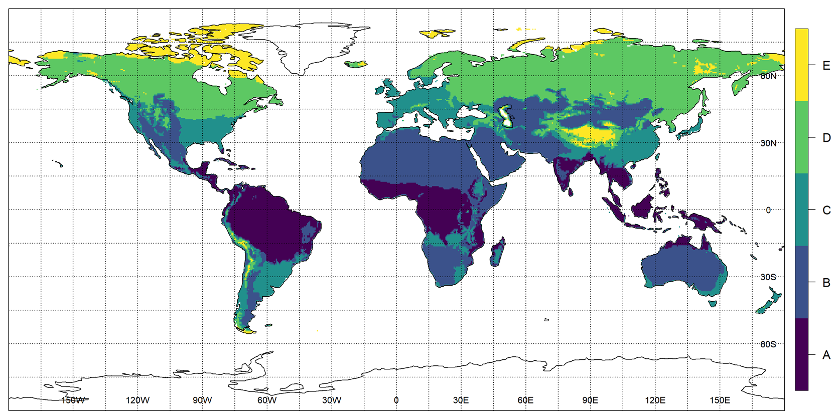
Figure 1 Köppen–Geiger climate zone classification with the five main zones: equatorial (A), arid (B), warm temperate (C), snow (D), and polar (E).

2.2 Water balance equation

TWS changes are closely related to precipitation via the water balance equation:

$$\begin{array}{}\text{(1)}& \mathrm{d}s/\mathrm{d}t=P-\mathrm{ET}-R,\end{array}$$

where $\mathrm{d}s/\mathrm{d}t$ is storage change with time, P is precipitation, ET is evapotranspiration, and R is runoff, all usually given in millimeter-equivalent water height per month (mm per month).

Any storage changes with time ($\mathrm{d}s/\mathrm{d}t$) must be caused by a water flux, which might be vertically between the surface and atmosphere (P or ET). Horizontal fluxes at or underneath the Earth's surface are summarized as lateral runoff (R). Since gravity missions directly observe TWSAs relative to an (undefined) long-term mean value, they can be used to derive information about water fluxes at a wide range of timescales. In principle, the difference between two storage estimates separated by 30 d (the usual sampling of the GRACE solutions) allows us to derive quantitative information about the amount of precipitation that occurred during this time span.

2.3 Deviation of storage (dTWSA)

Understanding the magnitude of water deficits remains crucial for determining drought recovery timelines. These water deficits can be directly inferred from the variability in TWSA data (Thomas et al., 2014). First, TWSA is smoothed by a 3-month moving average filter to reduce the high-frequency noise (Singh et al., 2021), resulting in smoothed TWSA (sTWSA). Variations in water storage can be influenced by long-term factors, such as glacier mass accumulation and/or groundwater extraction. To isolate the impact of such long-term processes, we detrended the TWSA data for each grid by removing the linear trend of the relevant grid (Singh et al., 2021). Detrending removes the linear trend, essentially isolating the deviations from this long-term trend, which we refer to as deviation of storage (dTWSA):

$$\begin{array}{}\text{(2)}& {\mathrm{dTWSA}}_{x,y,t}={\mathrm{sTWSA}}_{x,y,t}-\mathrm{trend}\left({\mathrm{sTWSA}}_{x,y,t}\right),\end{array}$$

where ${\mathrm{sTWSA}}_{x,y,t}$ is the smoothed TWSA at the x,y grid point and time t, and $\mathrm{trend}\left({\mathrm{sTWSA}}_{x,y,t}\right)$ is the trend of the smoothed TWSA at the x,y grid point and time t.

2.4 Cumulative detrended precipitation anomaly (cdPA)

To ensure consistency with dTWSA, we perform a temporal integration of the precipitation data. Then, cumulative precipitation anomalies (cPAs) were obtained by subtracting the mean precipitation observed from April 2002 to December 2020 (reference period) from the actual precipitation data for each product:

$$\begin{array}{}\text{(3)}& {\mathrm{cPA}}_{x,y,t}={\mathrm{cP}}_{x,y,t}-\stackrel{\mathrm{‾}}{{\mathrm{cP}}_{x,y}},\end{array}$$

where ${\mathrm{cP}}_{x,y,t}$ is the cumulated precipitation at the x,y grid point and time t, and ${\stackrel{\mathrm{‾}}{\mathrm{cP}}}_{x,y}$ is the temporal mean of the cumulative precipitation at the x,y grid point.

Similar to dTWSA, we smoothed the cumulative precipitation anomalies (scPAs) derived from GPCC and GPCP by applying a 3-month moving average filter (Singh et al., 2021). This process effectively reduced short-term fluctuations or noise in the anomaly data. To isolate variations in precipitation anomalies from long-term trends, we further detrended the smoothed precipitation anomalies. This additional step reduced any remaining long-term trends in the precipitation patterns. Finally, the cumulative detrended precipitation anomaly (cdPA) data were obtained:

$$\begin{array}{}\text{(4)}& {\mathrm{cdPA}}_{x,y,t}={\mathrm{scPA}}_{x,y,t}-\mathrm{trend}\left({\mathrm{scPA}}_{x,y,t}\right),\end{array}$$

where ${\mathrm{scPA}}_{x,y,t}$ is the smoothed precipitation anomalies at the x,y grid point and time t, and $\mathrm{trend}\left({\mathrm{scPA}}_{x,y,t}\right)$ is the trend of the smoothed precipitation anomalies at the x,y grid point and time t.

2.5 Relationship between dTWSA and cdPA

Variations in the key water fluxes (ET, R, and P) cause fluctuations in TWS, a crucial component of the water budget equation. This study leveraged the assumption of a constant relationship between precipitation and the combined evapotranspiration and runoff (ET + R) flux. This assumption allows us to infer potential variations in precipitation based on changes in TWSA.

This predictive model enables us to estimate the amount of precipitation necessary to balance a water storage deficit. This approach offers a valuable tool for understanding and managing water resources by directly linking precipitation dynamics to changes in TWSA. A linear relationship between dTWSA and cdPA was established to estimate the required precipitation amount as follows:

$$\begin{array}{}\text{(5)}& \mathrm{cdPA}={\mathit{\beta }}_{\mathrm{0}}+{\mathit{\beta }}_{\mathrm{1}}\cdot \mathrm{dTWSA}+\mathit{\epsilon },\end{array}$$

where β₀ is the intercept, β₁ is the slope (regression coefficient), and ε represents the residual errors of the fit.

The units of cdPA and dTWSA are both in mm per month. Therefore, a β₁ value of 1 signifies that cdPA is well represented by dTWSA. In regions where β₁ equals 1, precipitation changes directly translate to storage variations. Conversely, regions with β₁ greater than 1 indicate that some of the local precipitation is immediately transported away and does not change the local storage. This suggests that the variability in storage data only partially captures all precipitation due to other hydrological processes (e.g., ET and R) in these regions. Regions with β₁ less than 1 suggest that a smaller amount of precipitation than needed is sufficient to address the storage deficit. In other words, there must be either additional inflow from other places that is phase locked with local rain events or severe positive biases in rainfall as seen by GPCC or GPCP, leading to an underestimation of the precipitation required based solely on storage variations (Singh et al., 2021).

Following the study of Singh et al. (2021), we estimated not only regression coefficients (i.e., β₀ and β₁), but also Pearson's correlation coefficient (r) between cdPA and dTWSA, as well as maximum drought length over each pixel, utilizing 19 years of monthly data (i.e., between 2002 and 2020). We classified the correlation coefficient values as follows: no or insignificant correlation (0.00–0.13), weak correlation (0.14–0.39), moderate correlation (0.40–0.69), and strong correlation (0.70–1.00). Here, a positive relationship is expected between cdPA and dTWSA such that positive (negative) precipitation anomalies should lead to increased (decreased) storage changes. Reverse signs in cdPA and dTWSA anomalies indicate weak or no linear relationship between the two variables. Accordingly, the study of Singh et al. (2021) eliminated the pixels that contain weak or no linear relationship between cdPA and dTWSA (i.e., r < 0, β₁ < 1, and maximum drought length < 5 months) from the global analyses. Sampling errors could cause fluctuations around 1, and random variability may cause some of the pixels to have β₁ values slightly less than 1, while these pixels may still have some considerable linear relationship. Accordingly, while the methodology of Singh et al. (2021) masked out regions with β₁ <1, in this study, regions with β₁ < 0 are masked out in addition to regions with r < 0 and maximum drought length < 5 months.

2.6 DRT

Both TWSA and P are used to quantify DRT. We closely follow the methodology given by Singh et al. (2021) and utilize two different methods to estimate DRT. The first method, based on storage deficit, utilizes only GRACE data to quantify DRT as the duration of the residuals of TWSA from its climatology. The second method is based on the required precipitation amount derived from both TWSA and precipitation datasets. In this approach, a drought is considered to end when the absolute required precipitation amount surpasses the observed precipitation amount. We thus utilize two different precipitation products (GPCC and GPCP), two different GRACE storage estimates (G3P and JPL mascon), and two different DRT estimation methods (storage deficit and required precipitation amount) to study the consequences of those processing choices for different climate zones as defined by the Köppen–Geiger climatology (in total, eight different DRTs are calculated).

2.6.1 DRT based on storage deficit

The deviation of TWSA from its climatology can offer valuable insights into drought characteristics. To calculate this deviation, we first create a reference point by averaging TWSA values for each month across the entire time series. For example, to establish the average January TWSA, we would calculate the mean of all January values in the data. This average monthly TWSA represented the climatology for that specific month. Subsequently, we calculated how much each TWSA data point deviated from this average climatology by subtracting the corresponding monthly climatology value. To identify drought events, we first calculated a climatology (long-term average) for TWSA data from both JPL mascon and G3P products using the time series from April 2002 to December 2020. This climatology serves as a reference point for typical TWSA conditions for each month. We then subtracted the corresponding monthly climatology value from each TWSA data point, resulting in residuals. Negative residuals indicate water storage deficits (Thomas et al., 2014). We classified periods with persistent negative residuals lasting longer than 3 consecutive months as drought events, signifying prolonged periods of below-average water storage (Singh et al., 2021). Negative residuals lasting less than 3 consecutive months were not classified as droughts. However, if a new negative residual period began within 1 month of a previous drought recovery, we considered them a continuation of the same drought event. This approach ensured a cohesive record of drought occurrences over time. By applying these criteria, we were able to establish a comprehensive inventory of drought characteristics for each grid point. This inventory served as the basis for our DRT estimation using the storage deficit method. This method analyzed the duration of negative residuals (i.e., smaller storage values than usual) of dTWSA at each location and time, thereby providing insights into the temporal patterns and the severity of drought events.

2.6.2 DRT based on required precipitation amount

The required precipitation amount is obtained from the linear relationship between dTWSA and cdPA. The storage deficit amount is represented by dTWSA, while cdPA, the output of this relationship, represents the required precipitation amount. To quantify the absolute required precipitation amount, the climatology of precipitation over each pixel was added back into the estimated required precipitation amount. The DRT estimation was then conducted by analyzing the duration during which the observed precipitation amount exceeded the absolute required precipitation amount for any given time and location (Singh et al., 2021). This approach allows for a comprehensive assessment of DRT dynamics across the different regions and periods.

2.7 Accuracy analysis

2.7.1 Consistency in DRT estimates

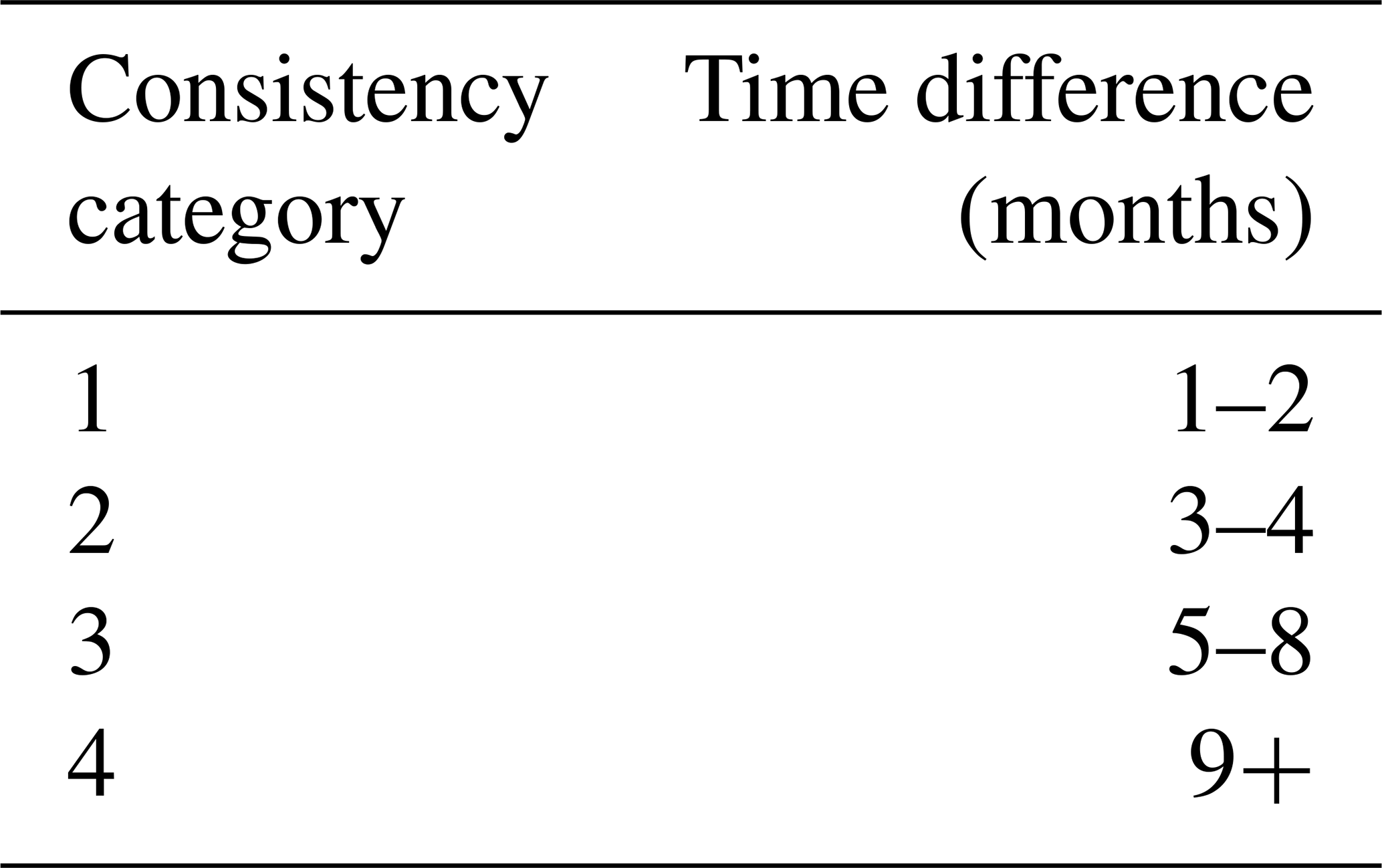
The consistency (level of agreement) between the two DRT estimates was quantified by assessing the differences in the timing obtained from both methods. In this context, consistency referred to the temporal difference between the estimated DRTs from each method, as categorized in Table 1. For example, if the time difference between the two methods fell within 1 or 2 months, the location was categorized as consistency category 1. By comparing the time differences between the DRT estimates from each method for each TWS–precipitation product, we were able to quantify the consistency between the two approaches. This analysis provides valuable insights into the reliability and robustness of the DRT estimates. In essence, it helped us assess how well the two methods converged on similar DRT values for the same locations.

Table 1 Consistency categories in DRT estimates.

2.7.2 Calculated statistics

In our analyses, we use standard error (SE) as a measure of the uncertainty associated with the means of our datasets. A smaller SE value indicates a more precise estimate of the mean DRT over each pixel, which is often achieved with less variation in the data (Lee et al., 2015). The value of SE was separately calculated for each grid point and climate zone as follows:

$$\begin{array}{}\text{(6)}& {\mathrm{SE}}_{x,y}={\displaystyle \frac{{\mathrm{SD}}_{x,y}}{\sqrt{n_{x,y}}}},\end{array}$$

where SD_x,y is the standard deviation of DRT at the x,y grid point, and n_x,y is the length of the dataset at the x,y grid point. In addition to SE, we employed confidence intervals (CIs) to assess the uncertainty around the mean values of our datasets (Curran-Everett, 2008; Lee et al., 2015). CIs provide a range of values that are likely to contain the true population mean with a specified level of confidence (95% in our case) as follows:

$$\begin{array}{}\text{(7)}& {\mathrm{CI}}_{x,y}={\mathit{\mu }}_{x,y}\mp \mathrm{1.96}\cdot {\mathrm{SE}}_{x,y},\end{array}$$

where μ_x,y is the mean DRT at the x,y grid point, and SE is the standard error of DRT at the x,y grid point.

3 Results and discussions

3.1 Relationship between cdPA and dTWSA

Figure 2a illustrates the spatial distribution of correlation coefficients between dTWSA and cdPA for one selected data combination of dTWSA from G3P and cdPA from GPCP (from now on abbreviated as G3P–GPCP). G3P–GPCP was selected to show actual values since the coupled product had the highest correlation coefficient (0.30). All the correlation coefficient values less than 0.13 were not significant (p > 0.05; n= 216). Significant and moderate correlations were found over Australia (0.55), South America (0.46), and southern Africa (0.60), characterized by not only substantial water storage variations, but also dense in situ observing networks. Such relatively high correlations indicate substantial agreement in these areas. The negative correlations over polar regions (∼ 70 % of grids), where water storage decline is strong during and after the melting season without any direct relation to the incoming precipitation, are more than those over the other regions (∼ 10 % of grids). Similar disagreements were found in highly arid climates in northern Africa and central Asia, where water storage variations are minimal, and GRACE observations are most likely dominated by measurement noise.

In addition, Figure 2b–d show the spatial distribution of differences in these correlation coefficients for the other possible combinations relative to the results obtained for G3P–GPCP. When investigating the JPL mascon (Fig. 2c), we observed differences primarily in arid climates with generally smaller TWS variations and a consequently poor signal-to-noise ratio in the GRACE data, where processing choices (like spatially variable a priori constraints, as applied in the mascon) had a greater effect. GPCC (Fig. 2d, JPL mascon–GPCC) affected correlations to a larger extent than GPCP (Fig. 2c, JPL mascon–GPCP), in particular over places with less dense in situ networks. Given the standard deviation values of correlation differences (Fig. 2c and d) resulting from the use of GPCC instead of GPCP, the variability was higher in Fig. 2d (global average: 0.21) than in Fig. 2c (global average: 0.14). Higher correlations for GPCP confirm the added value of satellite observations in otherwise data-sparse regions (like the Congo Catchment in central Africa). However, we also find a number of places where GPCC fits GRACE better than GPCP does, which suggests that systematic deficits in satellite observations might also degrade the combined product in certain areas. Despite the differences identified above, we conclude that there is a strong relation between precipitation and storage monitored by satellite gravimetry, implying that GRACE observations should be used more frequently in the future for large-scale hydrometeorological research.

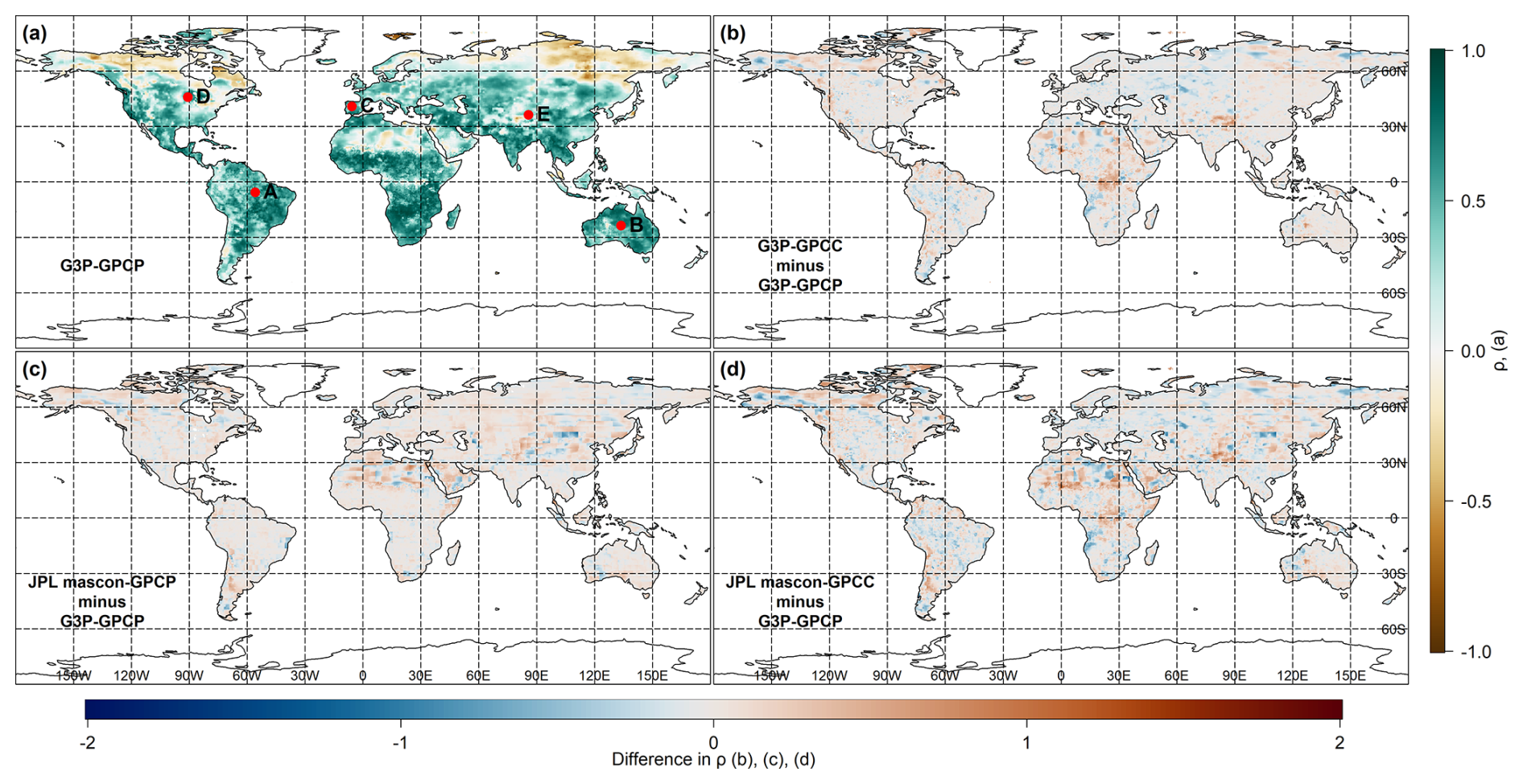
Figure 2 Representation of correlation coefficients between different dTWSA (i.e., G3P, JPL mascon) and cdPA (i.e., GPCP, GPCC) datasets. (a) Correlation coefficients obtained for dTWSA from G3P and cdPA from GPCP (G3P–GPCP). Differences in correlation coefficients relative to G3P–GPCP for (b) G3P–GPCC, (c) JPL mascon–GPCP, and (d) JPL mascon–GPCC. Note that regions with negative correlations were removed from subsequent analyses.

Figure 3a illustrates the spatial distribution of β₁ (Eq. 4), exceeding 0, for G3P–GPCP. We note that in certain regions of northern Africa, North America, and northeastern Asia, the β₁ value was less than 0. The values of TWS in these regions were likely influenced by factors other than precipitation, thereby making the link between precipitation and TWSAs less reliable. Most regions with polar climates (i.e., Köppen–Geiger Climate Zone E) exhibited β₁ below 0, indicating a weak link between precipitation anomalies and changes in TWS in these areas. Similar to the correlation analysis, a contrasting pattern emerged between the arid regions. North America's arid regions (i.e., Zone B) showed a pattern that was more comparable to Australia's arid regions. Africa's arid regions had a higher percentage of masked-out areas compared to those in Australia and North America. Additionally, the remaining areas in northern Africa's arid regions had lower β₁ values.

If we replace G3P with JPL mascon (Fig. 3c), we notice that β₁ values remain almost the same for the global average (mean difference of −0.01 in Fig. 3c). A quite similar pattern also emerges when using GPCC instead of GPCP (Fig. 3b), and the overall largest decreases in β₁ values are found for the G3P–GPCC combination (−0.06). In particular, using GPCP in Asia's snow zone and Australia's arid zone revealed more regions with β₁ closer to 1 than using GPCC. This suggests less necessity for additional variables to explain the relationship between precipitation anomalies and TWS changes in these regions when using GPCP instead of GPCC. In Europe's warm temperate zone, the use of the JPL mascon revealed more regions with β₁ larger than 3 compared to using G3P.

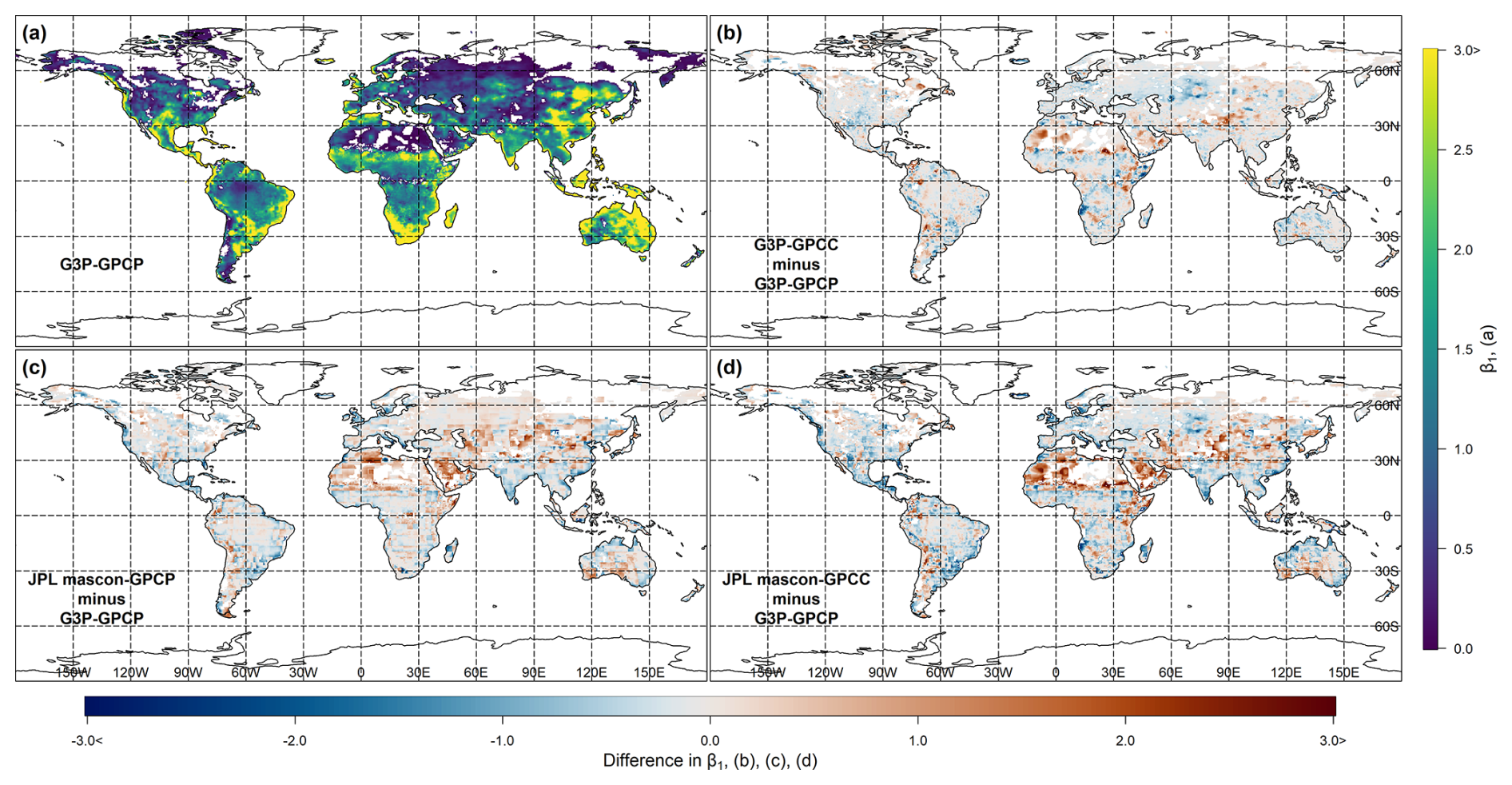
Figure 3 Representation of β₁ values between different dTWSA (i.e., G3P, JPL mascon) and cdPA (i.e., GPCP, GPCC) datasets. (a) β₁ values obtained for dTWSA from G3P and cdPA from GPCP (G3P–GPCP). Differences in β₁ values relative to G3P–GPCP for (b) G3P–GPCC, (c) JPL mascon–GPCP, and (d) JPL mascon–GPCC. Regions where the β₁ value is smaller than 0 are shown in white. Note that regions with β₁ values less than 1 were deemed as having a weak precipitation–storage relationship and were excluded from subsequent analyses.

Figure 4a displays a time series of dTWSA derived from both G3P and JPL mascon TWSA datasets in an example location in Australia (133.75° E, 16.75° S). Figure 4b illustrates the time series of cdPA derived from both GPCC and GPCP for the same point. These visualizations allow us to observe and analyze the fluctuations in water storage deviations and cdPA over time, providing insights into the dynamics of water availability and precipitation and potential drought recovery patterns. Close agreement is observed between the time series of G3P and JPL mascon and those of GPCC and GPCP, as well as between dTWSA and cdPA (average r= 0.65), as shown in Fig. 4.

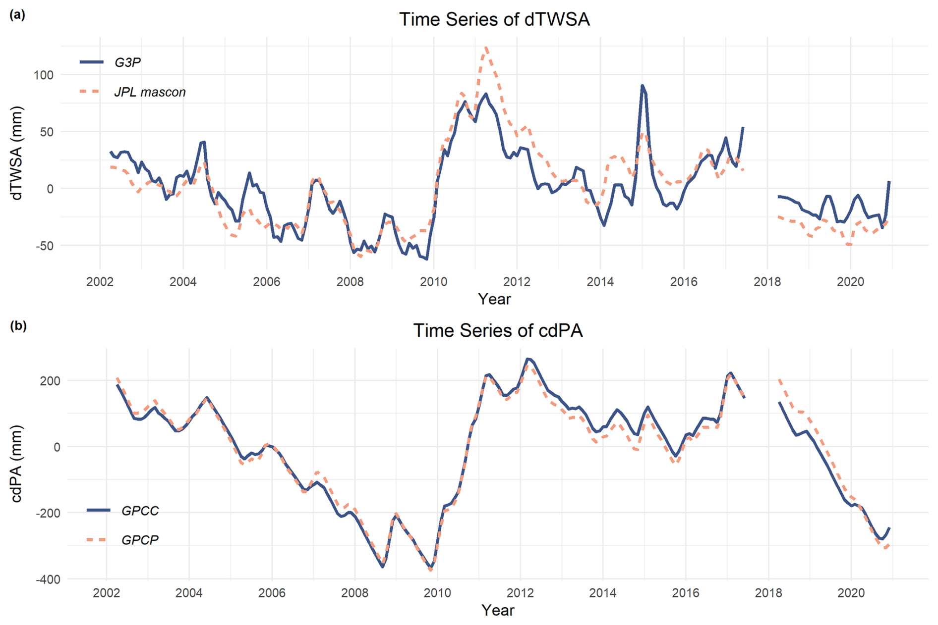
Figure 4 Time series of (a) dTWSA obtained from both G3P and JPL mascon products and (b) cdPA obtained from both the GPCC and the GPCP precipitation products, each in an example location in Australia (133.75° E, 16.75° S).

3.2 DRT estimates

The spatial distributions of mean DRT estimates based on storage deficit and required precipitation amount from the G3P–GPCP coupled product are shown in Figs. 5a and 6a, respectively. Figures 5b–d and 6b–d depict the spatial distribution of the differences between the mean DRT estimates derived from G3P–GPCP and G3P–GPCC and JPL mascon–GPCP and JPL mascon–GPCC, respectively, for both methods. The precipitation data are not utilized in calculating DRT estimates based on the storage deficit method (Fig. 5). However, they are used in the masking procedure for regions with weak or no linear relationship between cdPA and dTWSA. Although the unmasked regions have identical DRT values, the differences between Fig. 5a and b, as well as between Fig. 5c and d, arise from whether a region is masked or unmasked. Consequently, these figures are not identical. Even though the required precipitation method incorporated precipitation data into DRT estimates, the overall spatial patterns of mean DRT remained similar between G3P–GPCP and G3P–GPCC (Fig. 6b) as well as between JPL mascon–GPCP and JPL mascon–GPCC. Figures 5 and 6 indicate that both the mean and the spatial distributions of DRT estimates were consistent with each other using both methods.

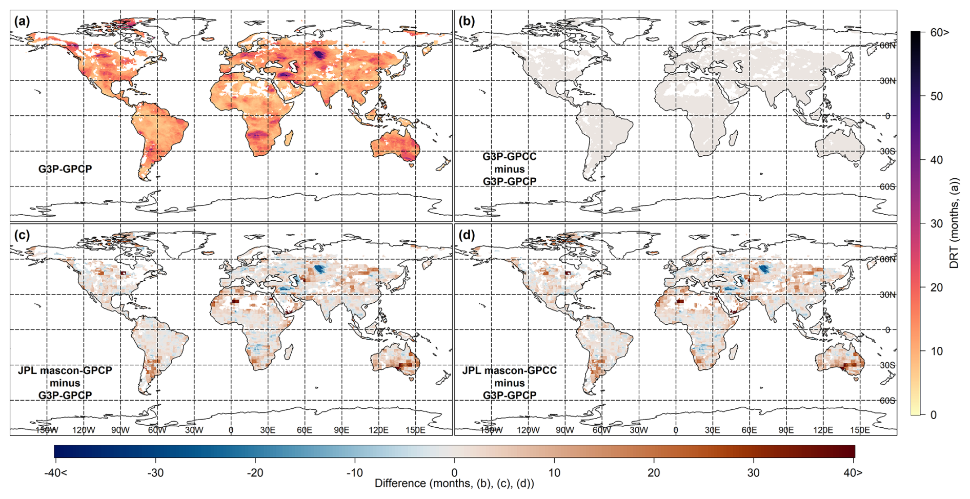
Figure 5 Representation of mean drought recovery time (DRT) estimates based on the storage deficit method, obtained from different dTWSA (i.e., G3P, JPL mascon) and cdPA (i.e., GPCP, GPCC) datasets. (a) DRT estimated using dTWSA from G3P and cdPA from GPCP (G3P–GPCP). Differences in DRT relative to G3P–GPCP for (b) G3P–GPCC, (c) JPL mascon–GPCP, and (d) JPL mascon–GPCC.

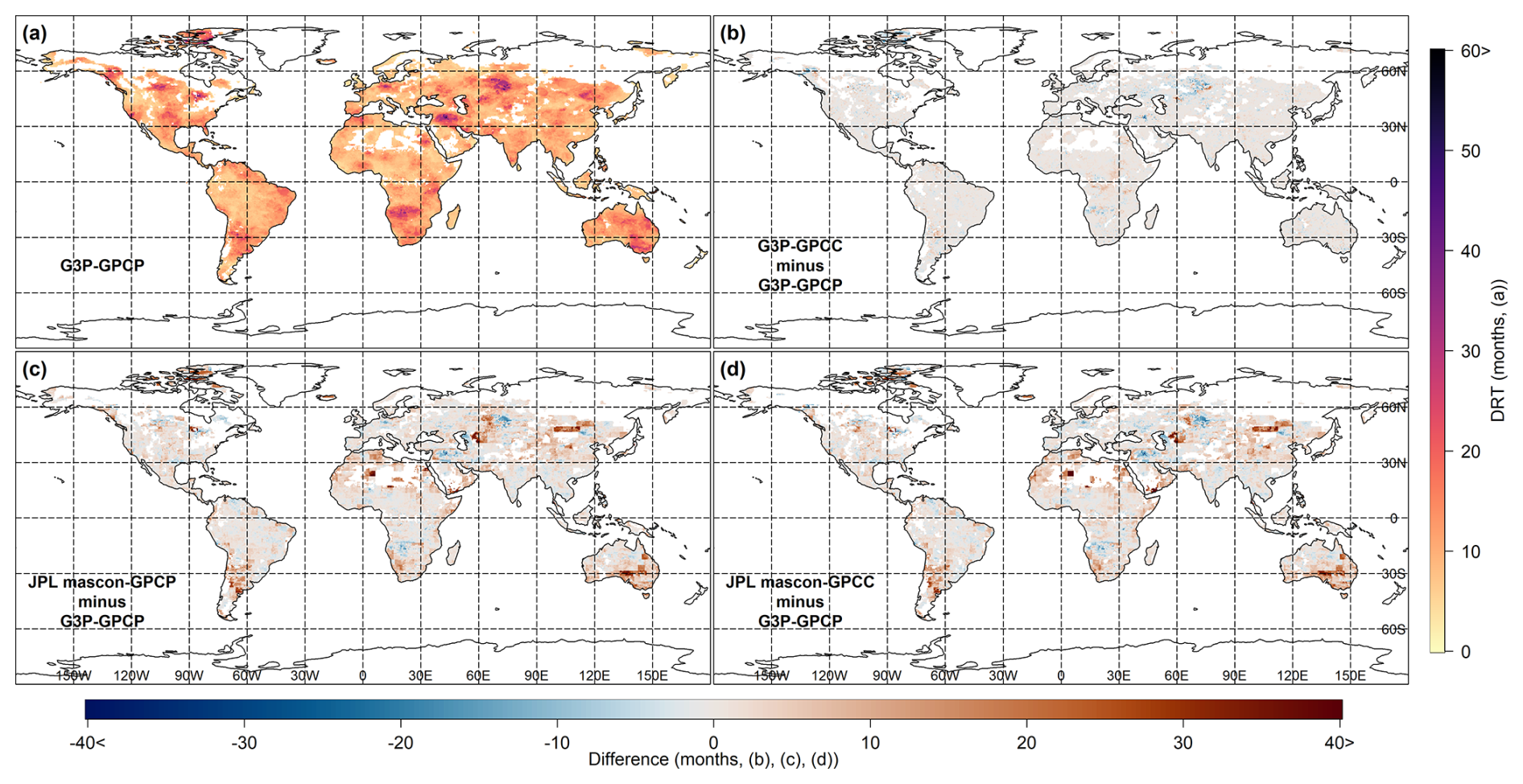
Figure 6 Representation of mean drought recovery time (DRT) estimates based on the required precipitation amount method, obtained from different dTWSA (i.e., G3P, JPL mascon) and cdPA (i.e., GPCP, GPCC) datasets. (a) DRT estimated using dTWSA from G3P and cdPA from GPCP (G3P–GPCP). Differences in DRT relative to G3P–GPCP for (b) G3P–GPCC, (c) JPL mascon–GPCP, and (d) JPL mascon–GPCC.

Figure 5a and b, which utilize G3P as the TWS product with GPCC and GPCP for precipitation, respectively, reveal the highest mean DRT (50–60 months) estimates based on the storage deficit method in Iran and central Asia. Likewise, for the required precipitation amount method, Fig. 6a and b, which also utilize G3P as the TWS product with GPCC and GPCP for precipitation, respectively, show the highest mean DRT in the same regions. Both methods consistently identified Iran, central Asia, southeastern Australia, and northern Africa as the regions experiencing the highest mean DRT (50–60 months), as illustrated in Fig. 5c and d and Fig. 6c and d, which utilize JPL mascon as the TWS product with GPCC and GPCP for precipitation, respectively. The spatial correlation between Figs. 5a and 6a is 0.75. This shows a high level of spatial correlation between the two DRT estimates based on the two methods.

The other regions that exhibited high DRT estimates based on both methods and across all the product combinations are central and southern South America (∼ 40 months), central and southern Africa (∼ 45 months), eastern Australia (∼ 35 months), central and western North America (∼ 40 months), central Europe (∼ 35 months), and eastern Asia (∼ 30 months). Increasing global aridity and drought areas since the mid-20th century, mainly as a result of extensive dryness in eastern Australia and northern mid-latitude regions, as reported by Dai (2011), are consistent with the findings of high DRT estimates of this study. Eastern Australia (∼ 35 months) experienced more severe drought conditions than western Australia (∼ 20 months) based on both methods. Consistent with the results of this study, previous research has focused on monitoring droughts in regions with a history of severe, multi-month drought events, such as Iran, central Europe, central and western North America, southeast Australia, and central South America, and which have experienced higher drought severity compared to other regions (Dai, 2011; Madadgar and Moradkhani, 2014; Rubel et al., 2017; Wu et al., 2023). Over the Colorado River basin (Madadgar and Moradkhani, 2014), droughts of varying severity were observed from 2001 to 2004, lasting a total of 48 months for the period from 2000 to 2011. Our findings for the same region indicate a mean DRT of approximately 30 months. The results of this study (Figs. 5a and 6a) are consistent with those of Boergens et al. (2020), which found that central Europe is a drought-prone region, experiencing extreme drought during the consecutive summers of 2018 and 2019, with recovery taking over a year. Moreover, the mean DRT estimates obtained from both methods when using JPL mascon were greater than those when using G3P. As shown in Fig. 6, the close agreement between GPCC and GPCP regarding the spatial distribution of mean DRT estimates for both TWS products (G3P and JPL mascon) indicates that the choice of precipitation product (GPCC or GPCP) may not influence the overall spatial patterns of DRT estimates. Figures A1 and A2 given in the Appendix illustrate the spatial distributions of the SE of DRT estimates, which were similar to the spatial distributions of the mean DRT estimates. Regions with the highest mean DRT also exhibited the highest SE, indicating that those experiencing longer DRT periods showed greater variability in the DRT estimates.

The mean DRT estimates based on storage deficit and required precipitation amount for the Köppen–Geiger main climate zones using all the TWS–precipitation coupled products are shown in Fig. 7a and b, respectively. Error bars representing the 95 % confidence intervals for each zone indicate variability in the mean DRT estimates, while the “n” values show the number of grids per coupled product within each zone. For both methods, the polar (E) zone exhibited the highest mean DRT (18.1 months for storage deficit, 14.2 months for required precipitation amount). Except for the polar (E) zone, consistent with previous findings (Van Lanen et al., 2013), for both methods, the arid (B) zone exhibited the highest mean DRT (14.8 months for storage deficit, 12.9 months for required precipitation amount), while the equatorial (A) zone displayed the lowest (10.9 months for storage deficit, 9.7 months for required precipitation amount). Mean DRT estimates based on storage deficit and required precipitation amount were 13.9 months and 11.4 months in the warm temperate (C) zone, respectively, whereas they were 14.1 months and 10.0 months in the snow (D) zone, respectively. In particular, all the climate zones except the polar (E) zone displayed minimal variability (< 0.2 months) in the mean DRT (indicated by narrow 95 % confidence intervals), suggesting low uncertainty. Overall, the difference between G3P and JPL mascon is the highest in the arid (B, 3.8 months) and polar (E, 5.7 months) zones, whereas the differences in the other zones are smaller than those in the arid (B) and polar (E) zones. Figure A3a and A3b show SE for the DRT estimates based on storage deficit and required precipitation amount, respectively, across the Köppen–Geiger climate zones for all the TWS–precipitation coupled products. The polar (E) zone had the highest SE for both methods, while the lowest SE varied depending on the product. SEs for GPCC and GPCP were similar except in the polar (E) zone. The JPL mascon estimates had slightly larger SEs than G3P for both methods.

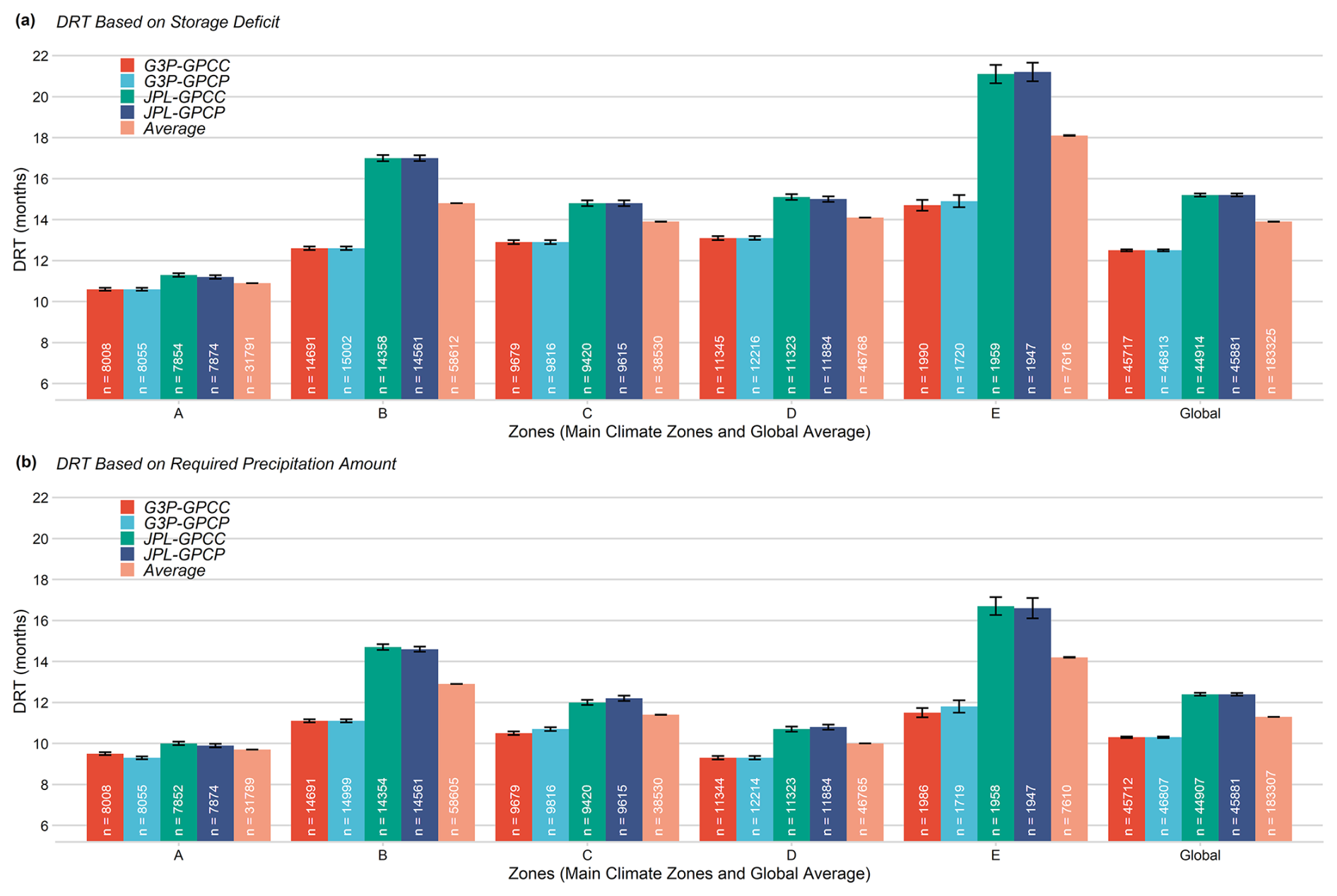
Figure 7 Average DRT estimates based on (a) storage deficit and (b) required precipitation amount for various climate zones from two different dTWSA (i.e., G3P and JPL mascon) and two different cdPA (i.e., GPCP and GPCC) products calculated for equatorial (A), arid (B), warm temperate (C), snow (D), and polar (E) climate zones, as given by the Köppen–Geiger classification.

On average, DRT based on storage deficit was estimated as 13.9 months, whereas DRT based on required precipitation amount was estimated as 11.3 months. When considering TWS products, regardless of the precipitation products, DRT estimates using JPL mascon (14.2 months) are consistently higher than those using G3P (11.6 months) across all the climate zones and the global average. When considering the precipitation products, DRT estimates using GPCC and GPCP yielded similar values (12.9 months) regardless of the TWS products across all the climate zones and the global average. These findings suggest that GPCC and GPCP closely agree on DRT estimates, and the storage deficit derived from G3P was consistently lower than that from JPL mascon across all the zones.

3.3 Consistency in DRT estimates

Figure 8a shows the spatial distributions of the consistency categories (Table 1) for the DRT estimates from G3P–GPCP coupled products. Figure 8b–d illustrate the spatial distributions of the differences in consistency categories for the DRT estimates between G3P–GPCP and G3P–GPCC, JPL mascon–GPCP, and JPL mascon–GPCC, respectively. Most regions fell into consistency category 1 (high agreement), and the mean absolute difference between DRT estimates calculated from both methods is 1.9 months. The spatial patterns were similar across all the possible data combinations (Fig. 8a–d), including those using the different TWS (G3P vs. JPL mascon) and precipitation (GPCC vs. GPCP) products. This consistency was also observed in the mean DRT for all the pairs. As expected, the regions in category 4 (time difference > 9 months) had the highest mean DRT and SE in both methods (Table 2).

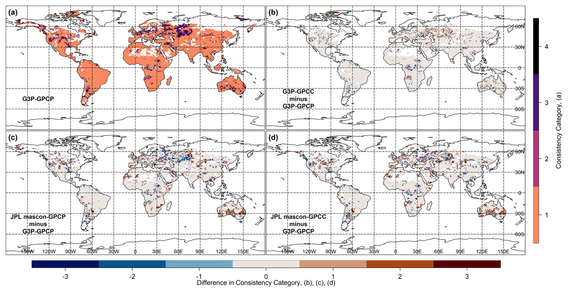
Figure 8 Representation of the consistency in DRT estimates (the class of the time difference in DRT values between two methods; see Table 1), obtained from the different dTWSA (i.e., G3P, JPL mascon) and cdPA (i.e., GPCP, GPCC) datasets. (a) Consistency using dTWSA from G3P and cdPA from GPCP (G3P–GPCP) and differences in consistency class relative to G3P–GPCP for (b) G3P–GPCC, (c) JPL mascon–GPCP, and (d) JPL mascon–GPCC.

Table 2 Mean DRT and SE for the consistency categories.

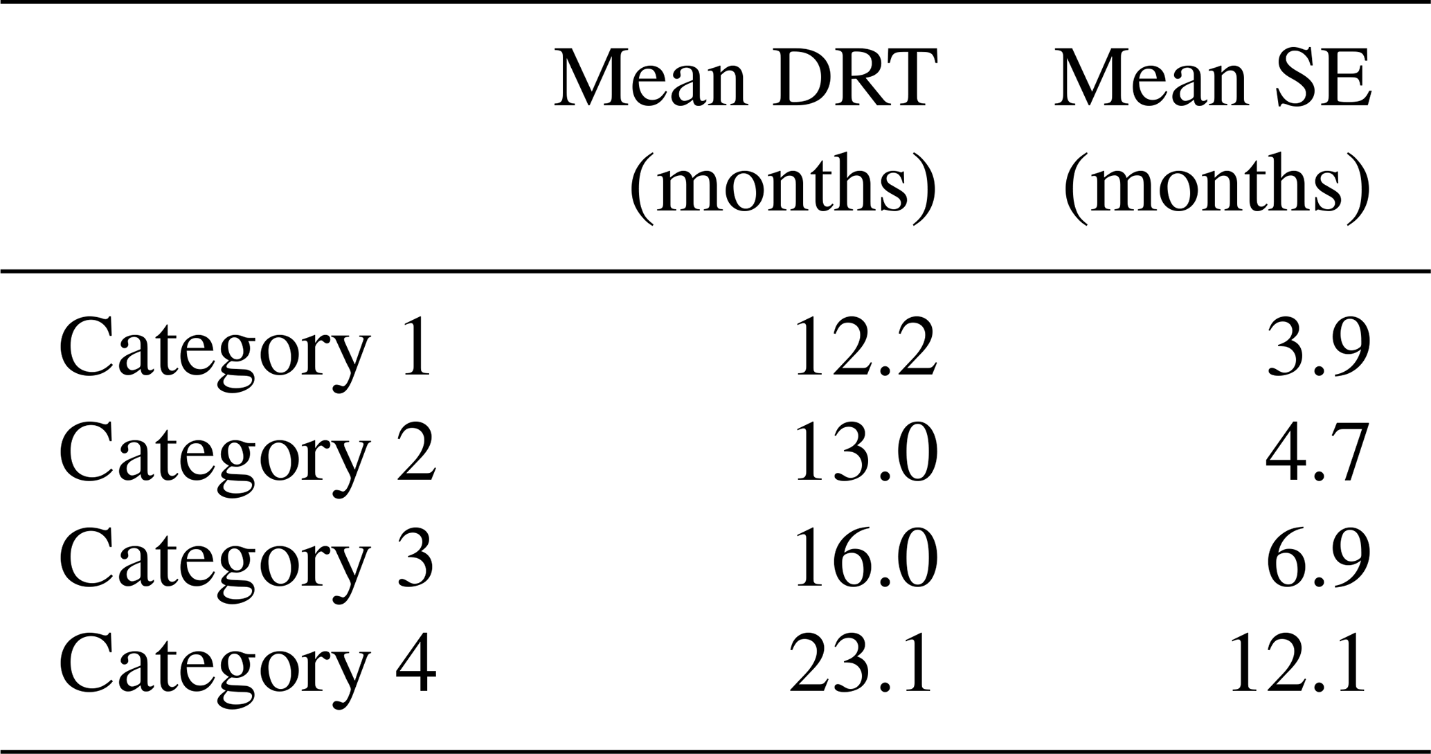
Figure 9 shows the consistency levels in terms of the percentage of category 1 (time differences of 1–2 months) for the Köppen–Geiger climate zones using all the coupled products. The polar (E) zone had the lowest average consistency (74.9 %), while the equatorial (A) zone had the highest (97.8 %). Overall, 87.5 % of DRT estimates achieved category 1 consistency. The consistency rate of G3P (88.5 %) is higher than that of JPL mascon (83.5 %) across the climate zones and globally. The G3P–GPCP combination achieved the highest consistency (on average, 88.7 %), whereas JPL mascon–GPCP showed the lowest (on average, 82.8 %).

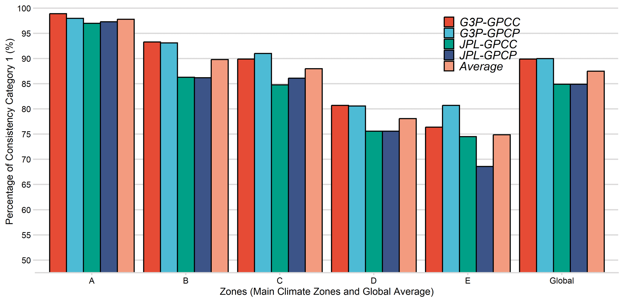
Figure 9 Percentage of DRT estimates whose consistency is category 1 for different climate zones using all the TWS–precipitation coupled products for climates characterized as equatorial (A), arid (B), warm temperate (C), snow (D), and polar (E) by the Köppen–Geiger classification.

The choice of the precipitation product (GPCC vs. GPCP) exerted minimal impact on consistency (average absolute difference 1.4 %) when the same TWS product was used. Conversely, G3P led to higher DRT consistency (average absolute difference 5.0 %) than JPL mascon when the same precipitation product was used. The climate zones also influenced consistency. GPCC and GPCP showed similar consistency in the arid (B, 0.2 months) zone and in the snow (D, 0.1 months) zone and the most different consistency in the polar (E) zone (5.1 % difference). In contrast, G3P and JPL mascon had the most similar consistency in the equatorial (A) zone (1.3 % difference) and the highest difference in the arid (B) zone and the polar (E) zone (7.0 % difference).

3.4 Discussion

Both precipitation products provided similar global mean DRT estimates (∼ 12 months), with a high consistency rate of 87.5%, suggesting that GPCC and GPCP are both reliable for global hydrological applications. The largest discrepancy in mean DRT estimation (0.1 months) was observed in the polar (E) zone, with no significant difference in the snow (D) zone. The consistency of the two precipitation products differed by less than 1 % across all the climate zones. These results for the precipitation products highlight the robustness of these products across the diverse climate zones.

For the TWS products, the global mean DRT estimation using JPL mascon (13.8 months) was 2.6 months higher than that using G3P (11.4 months). G3P exhibited 5.0 % higher global consistency (90.0 %) than JPL mascon (85.0%), suggesting that it is better suited for analyzing hydrological drought characteristics, particularly in regions with extreme climate conditions, such as the polar (E) and arid (B) zones, where G3P outperformed JPL mascon by 7.0 % in consistency. The significant disparity in mean DRT estimation in the polar zone (13.2 months for G3P versus 18.9 months for JPL mascon) highlights the challenges of accurately representing water storage dynamics in high-latitude regions, possibly due to differences in how the two products handle ice and snow storage variability. Conversely, the smallest differences in DRT estimates and consistency in the equatorial (A) zone suggest that both TWS products perform effectively in regions with stable precipitation patterns. These findings reveal that while both precipitation products perform similarly, G3P outperforms JPL mascon in consistency and alignment with TWS and precipitation-based DRT. This suggests that G3P may provide a more accurate representation of terrestrial water storage dynamics in diverse climate zones.

While this study demonstrates the utility of DRT estimates derived from precipitation and GRACE/GRACE-FO TWSA data for evaluating global datasets, it is essential to discuss certain methodological and data-related limitations to appropriately contextualize the findings. First, we assumed a linear relationship between cdPA and dTWSA. However, this dynamic relationship may be disrupted by anthropogenic activities (e.g., groundwater extraction, dam construction, deforestation, and urbanization) and natural processes (e.g., evapotranspiration and runoff), which can modify the hydrological response independently of precipitation dynamics. These factors may delay the transfer of precipitation into storage components or reduce the volume that ultimately contributes to storage. Second, uncertainties inherent to GRACE/GRACE-FO data processing and precipitation products, stemming from sensor characteristics or model parameterizations, may introduce noise or systematic biases into DRT estimates and their consistency. Third, the simplified water balance framework assumes stable partitioning of precipitation into evapotranspiration and runoff. However, temporal variability in these processes, driven by factors such as temperature, vegetation dynamics, or soil moisture conditions, may weaken the cdPA and dTWSA relationship, particularly in energy-limited regions (e.g., high-evapotranspiration zones) or areas highly sensitive to runoff (e.g., snowmelt-dominated basins). Fourth, a spatial-scale mismatch remains between datasets: GRACE/GRACE-FO's coarse spatial resolution smooths fine-scale TWS variability, while spatially aggregated precipitation data may obscure localized hydrometeorological events (e.g., intense convective rainfall), thereby affecting the precipitation–TWS relationship in regions characterized by complex topography or localized weather systems. Finally, the occurrence of high regression coefficients (β₁ > 2) highlights the sensitivity of storage changes to precipitation inputs and suggests the presence of unmodeled nonlinearities or time lags in the hydrological response. The high β₁ values, indicating rapid precipitation removal via runoff or evapotranspiration, may reflect limitations in the linear model's ability to capture delayed storage responses or nonlinearities in specific hydrological regimes. Despite these limitations, this study provides a valuable framework for assessing global precipitation and TWS products via hydrological drought characteristics.

4 Summary and conclusions

TWS changes from one time epoch to another, as observed by satellite gravimetry, are closely related to the precipitation amount occurring during that time interval. The novel observing concept realized by the GRACE and GRACE-FO missions thus provides a unique opportunity to evaluate the frequently used global precipitation products on monthly or longer timescales. GRACE/GRACE-FO directly provides water storage anomalies, offering a novel approach to characterizing drought by assessing the storage deficit. The time required for drought recovery can be directly derived from the temporal evolution of these deficits (Singh et al., 2021), enabling the measurement of both drought duration and severity.

Our assessments reveal that both GPCC and GPCP products exhibited not only similar DRT estimates but also comparable consistency globally and across all the Köppen–Geiger climate zones. However, as noted, GPCP's reliance on satellite data enhances its utility in data-sparse regions, making it a more versatile choice in such contexts. However, this advantage does not extend to regions with dense in situ networks, where the inclusion of satellite data does not improve its performance.

For TWS products, the mean DRT estimates from JPL mascon were, on average, 2.6 months higher than those from G3P, globally and across all the Köppen–Geiger climate zones. However, G3P showed slightly higher consistency in the DRT estimates (5.0 % difference, globally) than JPL mascon. Furthermore, G3P demonstrated greater consistency than JPL mascon across all the Köppen–Geiger climate zones. These findings highlight G3P's reliability for applications requiring precise water storage anomaly data, such as drought monitoring.

The results of our study underline the potential value of GRACE/GRACE-FO for hydrometeorological research due to the strong relationship between precipitation and TWS changes. Its global coverage (although with its rather low spatial resolution) allows for the testing of different precipitation products – not only those derived from combinations of satellite and in situ observations (as done in this study) but also those from numerical weather prediction models and global atmospheric reanalyses. Both NASA and the European Space Agency (ESA) are currently working on future satellite gravity missions with even more precise sensors and different orbital configurations to further enhance the quality of satellite gravimetry products for hydrological applications.

Appendix A

Abbreviations
cdPA	Cumulative detrended precipitation anomaly
cPA	Cumulative precipitation anomaly
DRT	Drought recovery time
dTWSA	Deviation of storage
G3P	Global Gravity-based Groundwater Project
GPCC	Global Precipitation Climatology Centre
GPCC FDM	Global Precipitation Climatology Centre Full Data Monthly Product
GPCP	Global Precipitation Climatology Project
JPL mascons	Jet Propulsion Laboratory mass concentration solutions
scPA	Smoothed cumulative precipitation anomaly
TWS	Terrestrial water storage
TWSA	Terrestrial water storage anomaly

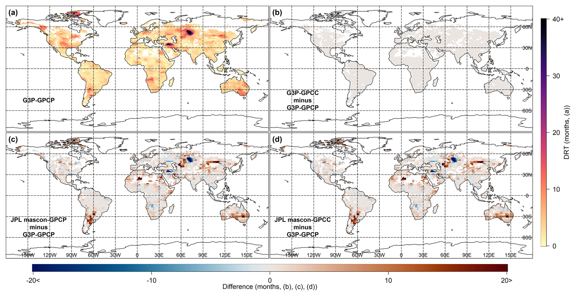
Figure A1 Display of the standard error in DRT estimates based on the storage deficit obtained from different dTWSA (i.e., G3P, JPL mascon) and cdPA (i.e., GPCP, GPCC) datasets. (a) Standard error for dTWSA from G3P and cdPA from GPCP (G3P–GPCP). Differences in standard error relative to G3P–GPCP for (b) G3P–GPCC, (c) JPL mascon–GPCP, and (d) JPL mascon–GPCC.

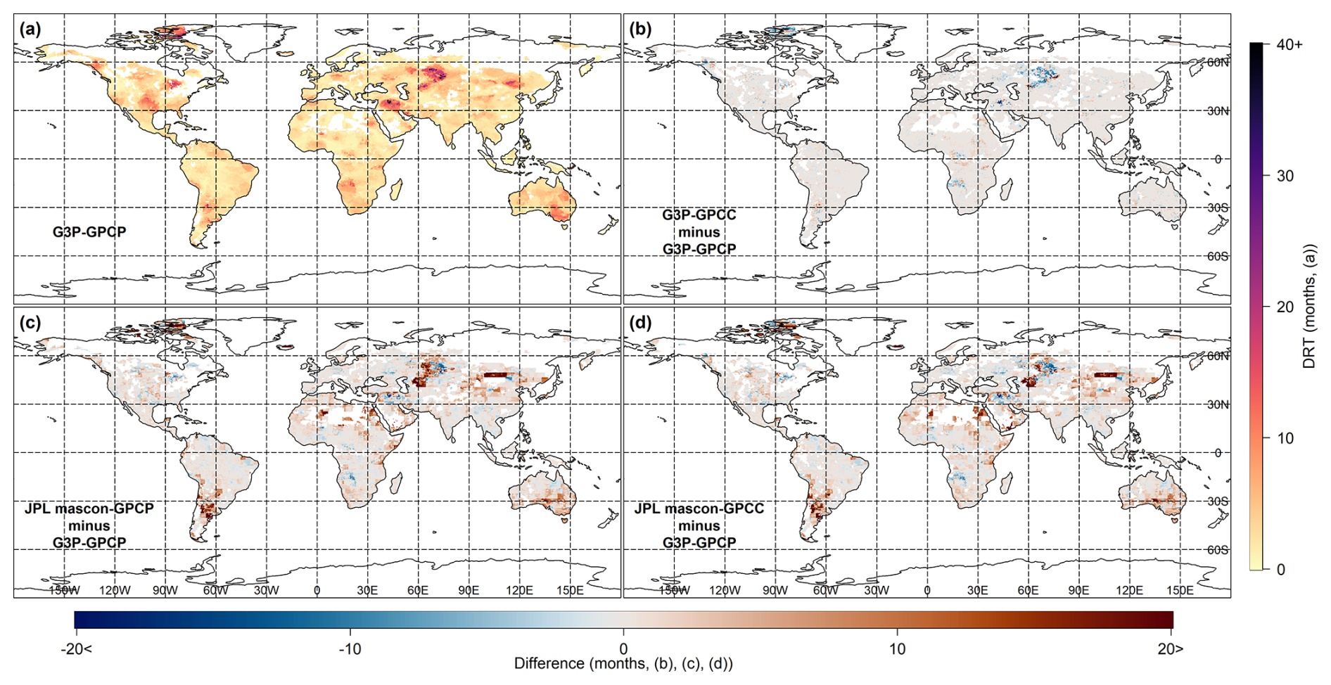
Figure A2 Display of the standard error in DRT estimates based on the required precipitation obtained from different dTWSA (i.e., G3P, JPL mascon) and cdPA (i.e., GPCP, GPCC) datasets. (a) Standard error for dTWSA from G3P and cdPA from GPCP (G3P–GPCP). Differences in standard error relative to G3P–GPCP for (b) G3P–GPCC, (c) JPL mascon–GPCP, and (d) JPL mascon–GPCC.

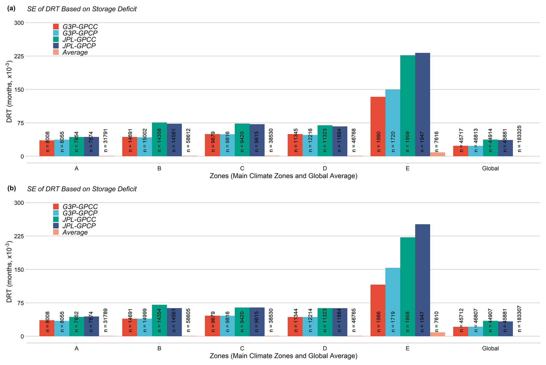
Figure A3 Standard error for average DRT estimates based on (a) storage deficit and (b) required precipitation amount for various climate zones from two different dTWSA (i.e., G3P and JPL mascon) and two different cdPA (i.e., GPCP and GPCC) products calculated for equatorial (A), arid (B), warm temperate (C), snow (D), and polar (E) climate zones, as given by the Köppen–Geiger classification.