Impacts of inter-basin water diversion projects on the feedback loops of water supply–hydropower generation–environment conservation nexus

To balance water resource distribution in different areas, inter-basin water diversion projects (IWDPs) have been constructed around the world. Unclear feedback loops of water supply–hydropower generation–environment conservation (SHE) nexus in IWDPs increase the uncertainty in rational scheduling of water resources for water receiving and water donation areas. To address the different impacts of IWDPs on a dynamic SHE nexus and explore synergies, a framework is proposed to identify these impacts across multiple temporal and spatial scales in a reservoir group. The proposed approach was applied to the Hanjiang River Basin (HRB) in China as a case study. Runoff series from the HRB at multiple temporal and spatial scales were provided through the Variable Infiltration Capacity hydrological model. Multi-level ecological flows were determined by the modified Tennant method based on a multi-level habitat condition method. 30 scenarios were set and modeled in a multisource input–output reservoir generalization model. Differences between scenarios were quantified with a response ratio indicator. The results indicate that without IWDPs there is negative feedback between water supply (S) and hydropower generation (H) and between S and environment conservation (E), while there is positive feedback between H and E. The negative feedback of S on H and the positive feedback of E on H are weakened or even broken in abundant-water periods. With IWDPs, water donation basins experience strengthened feedback loops, while water receiving basins experience weakened feedback loops. Feedback loops exhibit intrinsic similarity and stability across different time scales. Feedback loops in reservoirs with a regulation function remain stable under varying inflow conditions and feedback loops for downstream reservoirs are influenced by their upstream reservoirs, especially in low-flow periods. Simply increasing water receiving flow cannot resolve inherent SHE conflicts because of the persistent feedback polarity with IWDPs, and adaptive allocation rules are needed that account for these stable feedback patterns. The proposed approach can help quantify the impacts of IWDPs on SHE nexus and contribute to the sustainable development of SHE nexus.

1 Introduction

Water resources are fundamental to life, as well as economic and social development (MacGregor, 1963). Water supply, hydropower generation, and environment conservation constitute the three primary components of water resource utilization in a basin (Chung et al., 2021), delivering substantial economic, social, and ecological benefits to both humanity and nature. However, over the past 70 years, global water resources have been rapidly consumed and utilized, due to increasing human demand and climate change, leading to complex supply–demand conflicts (Tauro, 2021; Wang et al., 2024). Water supply, hydropower generation, and environment conservation compete, coordinate, and are interdependent with each other and intricate relationships can be found among them (Stickler et al., 2013). The interdependencies among these water supply (S), hydropower generation (H), and environment conservation (E) components are referred to as an SHE nexus (Endo et al., 2017; FAO, 2014; Sanders and Webber, 2012). Identifying the SHE nexus can elucidate the trajectory of water resource system evolution for various water resource management strategies, balance the relationships among water users, and promote sustainable resource use and ecological health (Mansour et al., 2024; Zhao et al., 2021).

Current studies on nexus primarily focus on the three fundamental resources: water, energy, and food (Conway et al., 2015; Quer et al., 2024; Wang et al., 2023). The SHE nexus refines the water–energy–food nexus and emphasizes basin-scale water resource management (Chen et al., 2020). Most studies on SHE nexus take reservoirs as nodes and primarily focus on multi-objective optimization of basin-wide water resource scheduling (Khalkhali et al., 2018; Qiu et al., 2021; Tang et al., 2024). Through game-theoretical analyses among components, they aim to identify feedback between paired components. From the perspective of reservoir nodes under scrutiny, current research primarily focuses on single reservoirs (Wu et al., 2021), virtual reservoirs (Chen et al., 2020), and cases of two connected reservoirs (Khalkhali et al., 2018). To optimize the allocation of basin-scale water resources, the deployment of cascade reservoir systems has increased significantly (Liu et al., 2022), wherein multiple reservoirs with different priority functions are strategically interconnected through series or parallel hydraulic linkages. These reservoirs form what we call a reservoir group. A reservoir group collaboratively manages the basin's water resource development and utilization. The different priority functions of reservoirs lead to different SHE nexus. It is conducive to deciphering the nexus of, and the directional changes within, an SHE system that the reservoirs are located in different locations within a basin, prioritizing different objective functions. Moreover, quantification of the E component often relies on the Tennant method (Tennant, 1976; Tharme, 2003) to estimate ecological flows (EFs) while neglecting temporal and spatial variations. Some of the E components only contain urban and rural ecological water use, and neglect the in-stream EFs (Chen et al., 2020). There is often not a straightforward positive or negative correlation between water supply, hydropower generation, and environment conservation components (Zitzler, 2007). The feedback loops among components can dynamically change when observed across different temporal and spatial scales (Keyhanpour et al., 2021). The components S, H, and E interact dynamically over time and space (Dong et al., 2019), inevitably leading to changes in the feedback loops of the resulting SHE nexus. However, studies on these changes in an SHE nexus are relatively scarce. Identifying synergy within competitive loops or competition within synergetic loops across various time–space scales enhances understanding of the dynamic changes in the SHE nexus and also provides strategies for dealing with competition among different users in actual water management. Therefore, it is critical to investigate the bidirectional and dynamic feedback loops of an SHE nexus across multiple temporal and spatial scales.

Due to frequent extreme events and intensive human activities, the spatial and temporal distribution of water resources exhibits more and more unevenness (Wang et al., 2024). The imbalance of water supply and demand has widely spread all over the world. Inter-basin water diversion projects (IWDPs), also commonly referred to as inter-basin water transfers (IBWTs, Dong et al., 2023; Sheng et al., 2024), have been widely implemented to solve the imbalance (Siddik et al., 2023) by transferring water resources from water-rich areas (i.e., water donating areas) to water-deficient regions (i.e., water receiving areas) through channels and other hydraulic engineering works. The IWDP initiatives seek to alleviate the imbalance among different basins but also result in notable changes in the water resource systems in both source and receiving areas (Long et al., 2020). Many studies have extensively examined the receiving effects of IWDPs on the three components (Tang et al., 2022; Tao et al., 2008; Wei et al., 2024), as well as focusing on the comprehensive evaluation of water resource systems (Kattel et al., 2019; Zhao et al., 2017) and multi-factor risk assessment of water donating areas (Bai et al., 2023; Mu et al., 2024; Yang et al., 2023) at different temporal and spatial scales. It was found that the dynamic planning and operation of IWDPs exert significant external impacts on an SHE system, inevitably leading to the system's “change–response–reconstitute” process. These impacts have changed the feedback loops among components of SHE systems. Additionally, studies have primarily emphasized single water donating or receiving impacts, overlooking the different impacts of IWDPs on SHE nexus and the comprehensive effects of multi-IWDPs. Water management regulations for IWDPs have become one of the focuses in SHE nexus studies (Mok et al., 2015). Current studies on this issue have primarily sought optimal water allocation methods for negotiations among water users in donating and receiving areas. They often employ case study approaches (e.g., interviews, field studies, policy reviews, and surveys) (Zhao et al., 2017) or inter-basin water resource allocation models (Ouyang et al., 2020; Wu et al., 2022). However, most of these studies have still oversimplified the interactions among these three components as only competitive (Yan et al., 2020). Identifying the changes in the feedback loops with IWDPs and synergies following the feedback loop changes are crucial steps in improving water dispatching and management in both donating and receiving areas.

One of the aims of this study is to identify the different impacts of IWDPs across multiple temporal and spatial scales on a dynamic SHE nexus in a reservoir group with different priority functions. Another is to explore a way to search synergies in the feedback loops of an SHE nexus. The research framework and methods are presented in Sect. 2, and our case study to verify the proposed framework is detailed in Sect. 3. Section 4 covers the results and Sect. 5 provides a comprehensive discussion. Conclusions are drawn in Sect. 6. All abbreviations used in this paper are listed in Table S6 in the Supplement.

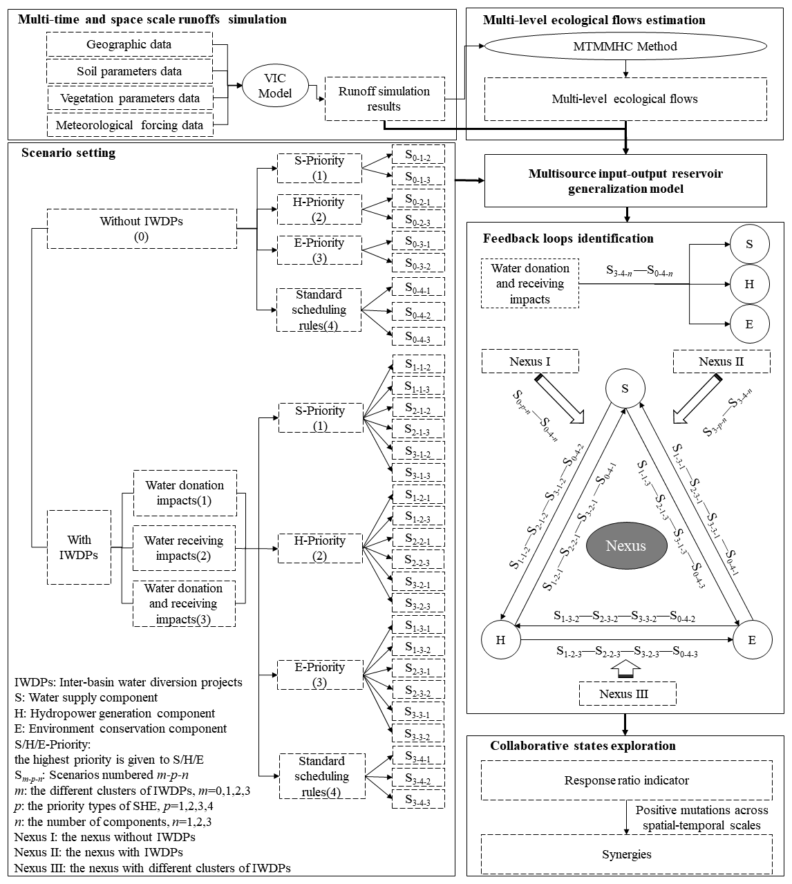
Figure 1 Framework to identify the impacts of different IWDPs on the feedback loops of SHE nexus.

2 Methodology

2.1 Research framework

To address the impacts of IWDPs across multiple temporal and spatial scales on dynamic SHE nexus, multiple temporal and spatial scale runoff simulations from the water donating basins are provided through a distributed hydrological model. Multi-level ecological flows and their corresponding multi-level ecological flow standards are also determined according to an available method with spatial–temporal variability. To facilitate identification of the impacts of IWDPs on SHE nexus, scenario experiments are set as “with/without IWDPs.” In order to take the different clusters of IWDPs into account, scenario experiments are classified by the impacts of IWDPs on a water donation area, on a water receiving area, or on an area with both water donation and water receiving if there are IWDPs. To evaluate the feedback loops of the SHE nexus, the priority order of S, H, and E is iteratively set in all reservoir nodes. We set different types of the highest priority in S, H, and E and take the standard scheduling rules as reference scenarios. All scenarios are modeled in a multisource input–output reservoir generalization model, differences between scenarios are quantified with a response ratio indicator, and the feedback loops with the different impacts of IWDPs are identified through the response ratio indicator. To explore the synergies, a positive mutation in a response ratio across time–space is found between pairwise components of SHE. This framework can be applied globally to identify the feedback loops of the SHE nexus in basins with IWDPs. Thus, our research framework is illustrated in Fig. 1. Nexus I–III in Fig. 1 are defined as the nexus with IWDPs, the nexus without IWDPs, and the nexus with the different clusters of IWDPs.

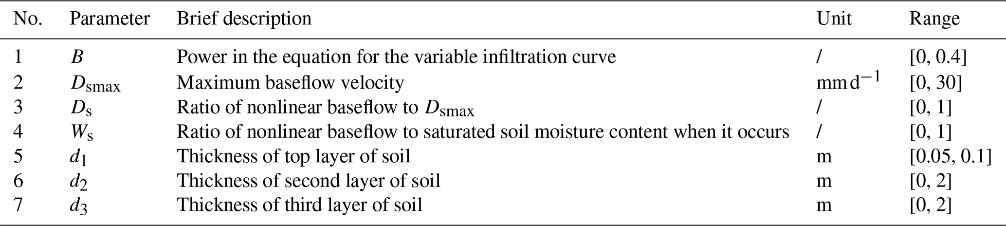
Table 1 Characteristics of parameters for model optimization (Gou et al., 2020).

2.2 The Variable Infiltration Capacity hydrological model

To simulate runoff results at multiple temporal and spatial scales, the Variable Infiltration Capacity (VIC) hydrological model is selected. The VIC model offers significant advantages in multiple temporal and spatial scale runoff simulations. It is a large-scale distributed hydrological model based on the spatial distribution grid of soil–vegetation–atmosphere transfer schemes (SVATS) (Liang et al., 1994), making it highly adaptable to studies at different spatial scales and supporting a wide range of input data types. The VIC model can simulate hydrological processes at various time scales, from hourly to annual, catering to different research needs. It has excelled at simulating both the energy balance and the water balance between the land and atmosphere, thereby addressing the oversight of energy processes in traditional hydrological models. The VIC model has been widely applied in runoff simulations across various basins worldwide, consistently yielding outstanding results (Wang et al., 2012; Yeste et al., 2024; Su et al., 2024). There are five steps to constructing a VIC model (Koohi et al., 2022): (1) collect and organize data; (2) preprocess the VIC model; (3) construct the VIC model of the selected basin; (4) run the catchment module; (5) conduct parameter calibration and validation. During the calibration process, important parameters highlighted in Table 1 are automatically calibrated using MATLAB to achieve the optimal parameter combination.

In order to verify the accuracy of the runoff simulation results, the simulations need to be compared with the observations. Three widely used quantitative indexes of numerical differences are selected and they are the Nash–Sutcliffe efficiency coefficient (NSE, Nash and Sutcliffe, 1970), coefficient of determination (R², Rousseeuw and Leroy, 1987), and percentage bias (PBIAS, Bland and Altman, 1986):

$$\begin{array}{}\text{(1)}& {\displaystyle }\mathrm{NSE}& {\displaystyle }=\mathrm{1}-{\displaystyle \frac{\sum _{t=\mathrm{1}}^T{\left(Q_t^{\mathrm{o}}-Q_t^{\mathrm{s}}\right)}^{\mathrm{2}}}{\sum _{t=\mathrm{1}}^T{\left(Q_t^{\mathrm{o}}-\stackrel{\mathrm{‾}}{Q^{\mathrm{o}}}\right)}^{\mathrm{2}}}},\text{(2)}& {\displaystyle }{R}^{\mathrm{2}}& {\displaystyle }={\displaystyle \frac{{\left[\sum _{t=\mathrm{1}}^T\left(Q_t^{\mathrm{o}}-\stackrel{\mathrm{‾}}{Q^{\mathrm{o}}}\right)\left(Q_t^{\mathrm{s}}-\stackrel{\mathrm{‾}}{Q^{\mathrm{s}}}\right)\right]}^{\mathrm{2}}}{\sum _{t=\mathrm{1}}^T{\left(Q_t^{\mathrm{o}}-\stackrel{\mathrm{‾}}{Q^{\mathrm{o}}}\right)}^{\mathrm{2}}\sum _{t=\mathrm{1}}^T{\left(Q_t^{\mathrm{s}}-\stackrel{\mathrm{‾}}{Q^{\mathrm{s}}}\right)}^{\mathrm{2}}}},\text{(3)}& {\displaystyle }\mathrm{PBIAS}& {\displaystyle }={\displaystyle \frac{\sum _{t=\mathrm{1}}^T\left(Q_t^{\mathrm{o}}-Q_t^{\mathrm{s}}\right)\times \mathrm{100}}{\sum _{t=\mathrm{1}}^T{Q}_t^{\mathrm{o}}}},\end{array}$$

where $Q_t^{\mathrm{o}}$ and $Q_t^{\mathrm{s}}$ are the observed and simulated runoff results at the tth month (m³ s⁻¹). $\stackrel{\mathrm{‾}}{Q^{\mathrm{o}}}$ and $\stackrel{\mathrm{‾}}{Q^{\mathrm{s}}}$ are the averages of, respectively, the observed and simulated runoff results over the whole period T (m³ s⁻¹). $\mathrm{NSE}\in (-\mathrm{\infty },\mathrm{1}]$: the closer NSE is to 1, the better are the simulations. An NSE of the simulations greater than 0.5 is acceptable. $R^{\mathrm{2}}\in [\mathrm{0},\mathrm{1}]$: R² approaching 1 means that the simulations are equal to the observations. PBIAS is utilized to quantify the cumulative deviation between the simulations and observations. PBIAS larger than 0 means that the simulations are generally small, and vice versa (PBIAS smaller than 0 means that the simulations are generally larger). When |PBIAS| < 25 %, the runoff simulation results are acceptable.

After getting the acceptable runoff simulation results at the selected hydrological stations, we estimate the runoff to reservoirs and the interval runoff of each pair of reservoirs according to the catchment area ratio of each reservoir with its upstream and downstream hydrological stations. The calculation formulas are as follows:

$$\begin{array}{}\text{(4)}& {\displaystyle }{Q}_{i,t}^{\mathrm{s}}& {\displaystyle }=\left\{\begin{array}{ll}\frac{Q_{\mathrm{d},\mathrm{1},t}^{\mathrm{s}}\times A_{\mathrm{1}}}{A_{\mathrm{d},\mathrm{1}}},& i=\mathrm{1},\\ Q_{\mathrm{u},i,t}^{\mathrm{s}}+\frac{\left(Q_{\mathrm{d},i,t}^{\mathrm{s}}-Q_{\mathrm{u},i,t}^{\mathrm{s}}\right)\times (A_i-A_{\mathrm{u},i})}{(A_{\mathrm{d},i}-A_i)},& i>\mathrm{1},\end{array}\right.\text{(5)}& {\displaystyle }\mathrm{\Delta }{Q}_{i,t}& {\displaystyle }=Q_{i,t}^{\mathrm{s}}-Q_{i-\mathrm{1},t}^{\mathrm{s}},i>\mathrm{1},\end{array}$$

where $Q_{i,t}^{\mathrm{s}}$ is the runoff to the ith reservoir at the tth period (m³ s⁻¹); $Q_{\mathrm{u},i,t}^{\mathrm{s}}$ and $Q_{\mathrm{d},i,t}^{\mathrm{s}}$ are the simulation runoff results of the upstream and downstream hydrological stations of the ith reservoir at the tth period (m³ s⁻¹); A_i is the catchment area of the ith reservoir (m²); and A_u,i and A_d,i are the catchment areas of the upstream and downstream hydrological stations (m²). ΔQ_i,t is the interval runoff of the ith reservoir at the tth period (m³ s⁻¹).

The inflow to the ith reservoir is the sum of the discharge from the (i−1)th reservoir and the interval runoff. The calculation formulas are as follows:

$$\begin{array}{}\text{(6)}& Q_{i,t}=\left\{\begin{array}{ll}{Q}_{\mathrm{1},t}^{\mathrm{s}},& i=\mathrm{1},\\ Q_{\mathrm{out},i-\mathrm{1},t}+\mathrm{\Delta }{Q}_{i,t},& i>\mathrm{1},\end{array}\right.\end{array}$$

where Q_i,t is the inflow to the ith reservoir at the tth period (m³ s⁻¹); $Q_{\mathrm{out},i-\mathrm{1},t}$ is the water release from the (i−1)th reservoir in period t (m³ s⁻¹).

2.3 Modified Tennant method based on multi-level habitat conditions

In order to establish a multi-level ecological flow standard to aid in evaluating river ecological health, the multi-level ecological flows are estimated by the MTMMHC method. There are over 200 methods for the estimation of ecological flows (EFs) worldwide, typically categorized into four types: hydrological, hydraulic, habitat simulation, and holistic (Tharme, 2003). The Tennant method, which determines EFs based on predetermined percentages of average annual flow, is the most widely used hydrological method (Tharme, 2003). The MTMMHC method (Li and Kang, 2014) modifies the Tennant method based on three parameters: average periodic flow, water period, and percentage. It can solve four key problems that exist in the current ecological flow standards: spatial transferability, monthly variability, inter-annual variability, and scalability (Li et al., 2015). Indeed, the MTMMHC method can avoid the impacts of extreme inter-annual flow events and uneven intra-annual distribution. This enables the calculation of different guarantee rates for various river sections, water years (e.g., wet, normal, and dry years), and months. It reflects the temporal and spatial variability of EFs and provides comprehensive and reasonable multi-level ecological flow standards. The steps of the MTMMHC method are as follows.

1. The year groups are divided into wet years (precipitation below the 25th percentile, P < 25 %), normal years (25 % ≤ P ≤ 75 %), and dry years (P > 75 %) first. Then a flow duration curve (FDC, Franchini et al., 2011) is constructed using the total-period method based on daily average flows simulated from 1976 to 2020 by the VIC model. Finally, the average of flows corresponding to the 90th and 95th percentiles of the FDC (Q_(90)xy and Q_(95)xy, m³ s⁻¹) for the yth month of the xth year is taken as the minimum ecological flow (MEF_xy, m³ s⁻¹). The formula is as follows:

   $$\begin{array}{}\text{(7)}& {\mathrm{MEF}}_{xy}={\displaystyle \frac{Q_{\left(\mathrm{90}\right)xy}+Q_{\left(\mathrm{95}\right)xy}}{\mathrm{2}}}.\end{array}$$

2. The MTMMHC method takes the 50 % flow of the FDC (Q_(50)xy, m³ s⁻¹) for the yth month of the xth year as the maximum optimum ecological flow (OEF_xy(max), m³ s⁻¹). According to the Tennant method, the EFs are assumed to be categorized in 10 levels, and the minimum optimum ecological flow (OEF_xy(min), m³ s⁻¹) is set as level 6. The formulas are as follows:

   $$\begin{array}{}\text{(8)}& {\displaystyle }{\mathrm{OEF}}_{xy(max)}& {\displaystyle }=Q_{\left(\mathrm{50}\right)xy},\text{(9)}& {\displaystyle }{\mathrm{OEF}}_{xy(min)}& {\displaystyle }={\displaystyle \frac{\mathrm{5}{Q}_{\left(\mathrm{50}\right)xy}+\mathrm{4}{\mathrm{MEF}}_{xy}}{\mathrm{9}}}.\end{array}$$

3. The MTMMHC method computes EFs at all levels using the arithmetic difference between MEF_xy and OEF_xy(min). The MTMMHC method eliminates the classification of OEF_xy(min) to OEF_xy(max), with the result that the grading number of EFs is R+1. The mode of all the grading numbers of selected stations is taken as the grading number R:

   $$\begin{array}{}\text{(10)}& {\displaystyle }R& {\displaystyle }=\text{Mode}\left(\text{Average}\right(m_{xy}\left)\right),\text{(11)}& {\displaystyle }{m}_{xy}& {\displaystyle }=\text{Round}\left({\displaystyle \frac{\mathrm{5}}{\mathrm{9}}}\times {\displaystyle \frac{Q_{\left(\mathrm{50}\right)xy}-{\mathrm{MEF}}_{xy}}{\mathrm{0.1}\times Q_{\left(\mathrm{50}\right)xy}}}\right)+\mathrm{1},\end{array}$$

   where m_xy is the grading number between MEF_xy and OEF_xy(min) in the yth month and xth year; Mode(⋅), Average(⋅), and Round(⋅) are the functions that return, respectively, the most frequently occurring number in Average(m_xy), the average of m_xy, and the nearest integer.

4. Based on the hierarchical idea of arithmetic progression, a range of EF criteria can be defined as follows:

   $$\begin{array}{}\text{(12)}& {\mathrm{EF}}_{xy\left(r\right)}={\mathrm{MEF}}_{xy}+{\displaystyle \frac{\mathrm{5}}{\mathrm{9}}}\times {\displaystyle \frac{r-\mathrm{1}}{R-\mathrm{1}}}\mathit{\pi }\left(Q_{\left(\mathrm{50}\right)xy}-{\mathrm{MEF}}_{xy}\right),\end{array}$$

   where EF_xy(r) is the rth-level ecological flow in the yth month of the xth year (m³ s⁻¹).

Figure 2 Multisource input–output flows for a single reservoir.

2.4 Log response ratio method for identifying feedback loops

2.4.1 Water supply, hydropower generation, and environment conservation indexes

To evaluate the state of S, H, and E, the water supply volume, hydropower generation, and ecological flow satisfaction rate, as indexes of the three components, are set. The formulas are as follows.

1. Regional water supply volume:

   $$\begin{array}{}\text{(13)}& \begin{array}{rl}{V}_{\mathrm{s},i,t}& =Q_{\mathrm{s},i,t}\times \mathrm{\Delta }t\\ & =V_{i,t}-V_{i,t+\mathrm{1}}+(Q_{\text{out},i-\mathrm{1},t}+\mathrm{\Delta }{Q}_{i,t}\\ & +Q_{\text{re},i,t}-Q_{\text{out},i,t}-Q_{\text{do},i,t})\mathrm{\Delta }t-I_{i,t}\end{array}\end{array}$$

   where $V_{\mathrm{s},i,t}$ is the regional water supply volume (m³); $Q_{\mathrm{s},i,t}$ is the regional water supply flow (m³ s⁻¹); Δt is the time interval (s); V_i,t and $V_{i,t+\mathrm{1}}$ are the storage volumes of the ith reservoir in, respectively, periods t and t+1 (m³); $Q_{\text{out},i-\mathrm{1},t}$ is the water release flow from the (i−1)th reservoir in period t (m³ s⁻¹); ΔQ_i,t is the flow of the intervening basin between the (i−1)th and ith reservoirs in period t (m³ s⁻¹); $Q_{\text{re},i,t}$ is the water receiving flow from IWDPs (m³ s⁻¹); $Q_{\text{do},i,t}$ is the water donation flow for IWDPs (m³ s⁻¹); and I_i,t is the sum of evaporation and seepage losses from the reservoir in period t (m³).

2. Hydropower generation:

   $$\begin{array}{}\text{(14)}& E_{i,t}=\sum _{t=\mathrm{1}}^T{N}_{i,t}\mathrm{\Delta }t,N_{i,t}=K_i{Q}_{\mathrm{e},i,t}{H}_{i,t},K_i={\mathit{\eta }}_{i}g\mathit{\rho },\end{array}$$

   where E_i,t is the hydropower generation of the ith reservoir (kW h); N_i,t is the output of the ith reservoir in the tth period (kW); K_i is the comprehensive hydropower coefficient of the ith reservoir ($\mathrm{kg}{\mathrm{s}}^{-\mathrm{2}}{\mathrm{m}}^{-\mathrm{2}}$); η_i is the hydropower generation efficiency; g is the gravitational acceleration (m s⁻²); ρ is the density of water (kg m⁻³); and $Q_{\mathrm{e},i,t}$ and H_i,t are, respectively, the release discharge for hydropower generation (m³ s⁻¹) and the average hydropower head of the ith reservoir in period t (m).

3. Ecological flow satisfaction rate is used to evaluate whether intra-river flow satisfies multi-level ecological flow standards. It is quantified through the segmented linear affiliation function:

   $$\begin{array}{}\text{(15)}& \begin{array}{rl}& {\mathrm{EFSR}}_{xy}=\\ & \left\{\begin{array}{ll}\begin{array}{c}\mathrm{0}\\ \frac{\mathrm{1}}{R+\mathrm{1}}\left(\frac{{\mathrm{EF}}_{xy}-\frac{E_{xy\left(\mathrm{1}\right)}}{\mathrm{2}}}{E_{xy\left(\mathrm{1}\right)}-\frac{E_{xy\left(\mathrm{1}\right)}}{\mathrm{2}}}\right)\end{array}& \begin{array}{c}{\mathrm{EF}}_{xy}\le \frac{E_{xy\left(\mathrm{1}\right)}}{\mathrm{2}}\\ \frac{E_{xy\left(\mathrm{1}\right)}}{\mathrm{2}}<{\mathrm{EF}}_{xy}\le E_{xy\left(\mathrm{1}\right)}\end{array}\\ \begin{array}{c}\frac{\mathrm{1}}{R+\mathrm{1}}+\frac{\mathrm{1}}{R+\mathrm{1}}\left(\frac{{\mathrm{EF}}_{xy}-E_{xy\left(\mathrm{1}\right)}}{E_{xy\left(\mathrm{2}\right)}-E_{xy\left(\mathrm{1}\right)}}\right)\\ \frac{\mathrm{2}}{R+\mathrm{1}}+\frac{\mathrm{1}}{R+\mathrm{1}}\left(\frac{{\mathrm{EF}}_{xy}-E_{xy\left(\mathrm{2}\right)}}{E_{xy\left(\mathrm{3}\right)}-E_{xy\left(\mathrm{1}\right)}}\right)\end{array}& \begin{array}{c}{E}_{xy\left(\mathrm{1}\right)}<{\mathrm{EF}}_{xy}\le E_{xy\left(\mathrm{2}\right)}\\ E_{xy\left(\mathrm{2}\right)}<{\mathrm{EF}}_{xy}\le E_{xy\left(\mathrm{3}\right)}\end{array}\\ \mathrm{\dots }& \mathrm{\dots }\\ \frac{R-\mathrm{1}}{R+\mathrm{1}}+\frac{\mathrm{1}}{R+\mathrm{1}}\left(\frac{{\mathrm{EF}}_{xy}-E_{xy(R-\mathrm{1})}}{E_{xy\left(R\right)}-E_{xy(R-\mathrm{1})}}\right)& E_{xy(R-\mathrm{1})}<{\mathrm{EF}}_{xy}\le E_{xy\left(R\right)}\\ \begin{array}{l}\frac{R}{R+\mathrm{1}}+\frac{\mathrm{1}}{R}\left(\frac{{\mathrm{EF}}_{xy}-E_{xy(R-\mathrm{1})}}{E_{xy\left(R\right)}-E_{xy(R-\mathrm{1})}}\right)\end{array}& \begin{array}{c}{E}_{xy\left(R\right)}<{\mathrm{EF}}_{xy}\le E_{xy\left(R+\mathrm{1}\right)}\end{array}\\ \mathrm{1}& E_{xy(R+\mathrm{1})}<{\mathrm{EF}}_{xy}\end{array}\right.\end{array},\end{array}$$

   where ${\mathrm{EFSR}}_{xy}\in [\mathrm{0},\mathrm{1}]$ is the ecological flow satisfaction rate in the yth month of the xth year. E_xy(1), E_xy(R), and E_xy(R+1) are MEF_xy, OEF_xy(min), and OEF_xy(max), respectively.

2.4.2 The multisource input–output reservoir generalization (MIORG) model for a reservoir group

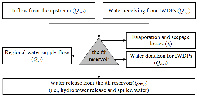
S, H, and E can be determined for reservoirs according to their scheduling rules. To quantify the differences of indexes with different impacts of IWDPs in reservoir nodes, MIORG models for a reservoir group are developed. For a single reservoir, the inputs generally refer to the inflow from upstream and the water receiving flow from IWDPs. The outputs from this MIORG model refer to regional water supply (i.e., domestic, industrial, and ecological water supply), water donation for IWDPs, evaporation and seepage losses, and water release from the reservoir. The multisource input–output to a single reservoir is shown in Fig. 2.

According to the principle of water balance, the MIORG model for a single reservoir is developed as follows:

$$\begin{array}{}\text{(16)}& V_{t+\mathrm{1}}=V_t+(Q_{\mathrm{in},t}+Q_{\text{re},t}-Q_{\mathrm{s},t}-Q_{\text{out},t}-Q_{\text{do},t})\mathrm{\Delta }t-I_t.\end{array}$$

Figure 3 Multisource input–output flows for reservoirs in a reservoir group.

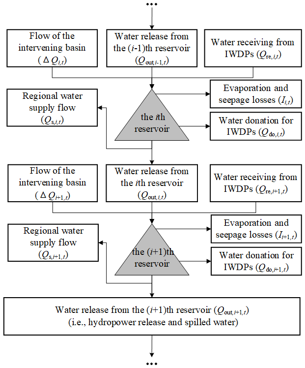
For a reservoir group, the inputs to the ith reservoir can be categorized as water release from the upstream reservoir (i.e., the (i−1)th reservoir), the flow of the intervening basin, and water receiving flow from IWDPs. The outputs from the ith reservoir in a reservoir group are the same as those from a single reservoir. The multisource input–output for the ith reservoir in a reservoir group is shown in Fig. 3. The MIORG model for the ith reservoir in a reservoir group is

$$\begin{array}{}\text{(17)}& \begin{array}{rl}{V}_{i,t+\mathrm{1}}=& V_{i,t}+(Q_{\text{out},i-\mathrm{1},t}+\mathrm{\Delta }{Q}_{i,t}+Q_{\text{re},i,t}\\ & -Q_{\mathrm{s},i,t}-Q_{\text{out},i,t}-Q_{\text{do},i,t})\mathrm{\Delta }t-I_{i,t}.\end{array}\end{array}$$

2.4.3 The log response ratio method

To analyze the feedback loops in Nexus I, Nexus II, and Nexus III in Fig. 1, the log response ratio (LRR) method (Patrick et al., 2022) is used to quantify the responses of S, H, and E for different clusters of IWDPs. This method captures nonlinear feedback loops within complex SHE nexus systems. The formula is as follows:

$$\begin{array}{}\text{(18)}& {\mathrm{LRR}}_n=\ln \left({\displaystyle \frac{(r_{c\left(n\right)}-r_n)+r_n}{r_n}}\right)=\ln \left({\displaystyle \frac{r_{c\left(n\right)}}{r_n}}\right),\end{array}$$

where LRR_n is the log response ratio of the nth component; n represents the performance evaluation component (1: water supply component; 2: hydropower generation component; 3: environment conservation component); LRR₁ refers to the log response ratio of the water supply volume between the two compared scenarios, characterizing the differences in the S component. Correspondingly, LRR₂ and LRR₃ represent, respectively, the differences in the H and E components between two compared scenarios. r_n is the value of regional water supply volume or hydropower generation or ecological flow satisfaction rate in the baseline scenario. r_c(n) is the value of the index in the compared scenario. r_c(n) and r_n are both greater than or equal to 0. A positive LRR_n indicates that r_c(n)>r_n, meaning that the compared scenario improves the component relative to the baseline. A negative LRR_n indicates that r_c(n)<r_n, meaning that the compared scenario worsens the component relative to the baseline. The absolute value of LRR_n reflects the degree of change on a logarithmic scale. The larger the absolute value of LRR_n, the more substantial the improvement (if positive) or worsening (if negative) is, measured logarithmically.

Table 2 The scenarios to identify the impacts of different clusters of IWDPs on the SHE nexus.

ISQ (in status quo) indicates that the component operates under the standard scheduling rules for reservoirs.

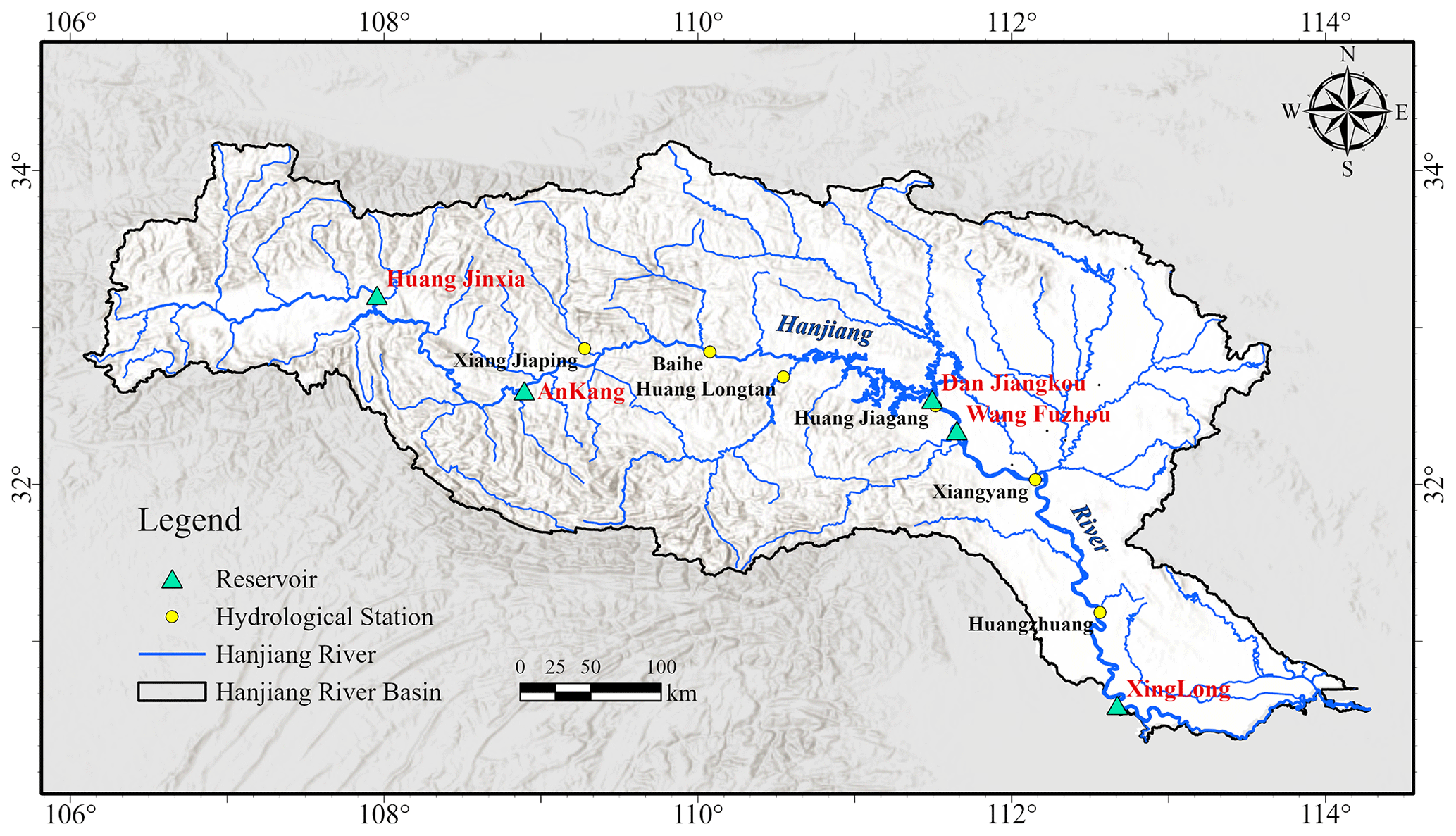
Figure 4 Overview map of the study area.

2.5 Scenario setting

To identify the impacts of different clusters of IWDPs on an SHE nexus, scenarios are set according to the following three aspects: with or without IWDPs (i.e., two types for IWDPs), different clusters of IWDPs (i.e., four clusters for each of the two types), and the priority orders of S, H, and E. As there are three components for the highest priority, six scenarios can be obtained through the combination of the three components. As S, H, and E are all determined from standard scheduling rules, there are also three types of standard scheduling rule. Combined with the types of different clusters of IWDPs, there will be a total of 30 scenarios (i.e., 4 clusters of IWDPs × 6 types for the highest priority combinations + 2 types for IWDPs × 3 types for standard scheduling rules), as listed in Table 2. Specifically, to iteratively set the priority orders of S, H, and E, all three components are all determined using standard scheduling rules first. Secondly, the highest priority is set to water supply (denoted as S-priority), which means that all reservoirs will first meet regional water demands (i.e., domestic, industrial, and ecological), with surplus water then allocated to hydropower generation and environment conservation needs. Additionally, increasing the regional water supply to 120 % enhances the observability and analytical prominence of the quantitative outcomes derived from these nexus. Thirdly, hydropower generation (H-priority) is prioritized to achieve the maximum output during the planned period. Finally, environment conservation (E-priority) is addressed by ensuring that the reservoir outflow meets OEF_xy(max). These scenarios offer flexibility in modeling SHE nexus system behavior under different conditions.

The scenarios are named using the format S_m-p-n, where m represents the different clusters of IWDPs (0: without IWDPs; 1: with only water donation; 2: with only water receiving; 3: with both donation and receiving); p represents the priority types of S, H, and E (1: the highest priority is water supply; 2: the highest priority is hydropower generation; 3: the highest priority is environment conservation; 4: standard reservoir scheduling rules); and n represents the performance evaluation component (1: water supply component; 2: hydropower generation component; 3: environment conservation component).

To analyze the feedback loops of an SHE nexus without IWDPs, the differences between the S_0-p-n (p = 1, 2, 3) and S_0-4-n scenarios are determined (i.e., the feedback loops of Nexus I, as shown in Fig. 1). To analyze the feedback loops with IWDPs (i.e., the feedback loops of Nexus II, as shown in Fig. 1), the differences between the S_3-p-n (p = 1, 2, 3) and S_3-4-n scenarios are determined. Thus, the differences between Nexus I and Nexus II show the impacts of IWDPs on the SHE nexus. To identify the SHE nexus with different clusters of IWDPs (i.e., the feedback loops of Nexus III, as shown in Fig. 1), the differences between S_m-p-n (m = 1, 2, 3; p = 1, 2, 3) and S_0-4-n scenarios are determined. The differences between Nexus I and Nexus III show the impacts of different IWDP clusters on the SHE nexus. S_0-4-n (i.e., the scenarios with standard scheduling rules without IWDPs) and S_3-4-n (i.e., the scenarios with standard scheduling rules with IWDPs) are the baseline scenarios for distinguishing Nexus I, Nexus III, and Nexus II. In the same way, to clarify the impacts of IWDPs on the three components, the differences between the S_0-4-n and S_3-4-n scenarios are determined.

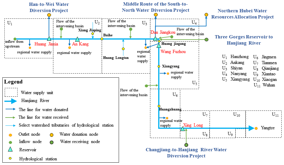
Figure 5 Sketch graphic of the Hanjiang River Basin (adapted from Zeng et al., 2023).

Table 3 Characteristic parameter values of reservoirs.

3 Study area and data

3.1 Overview of the study area

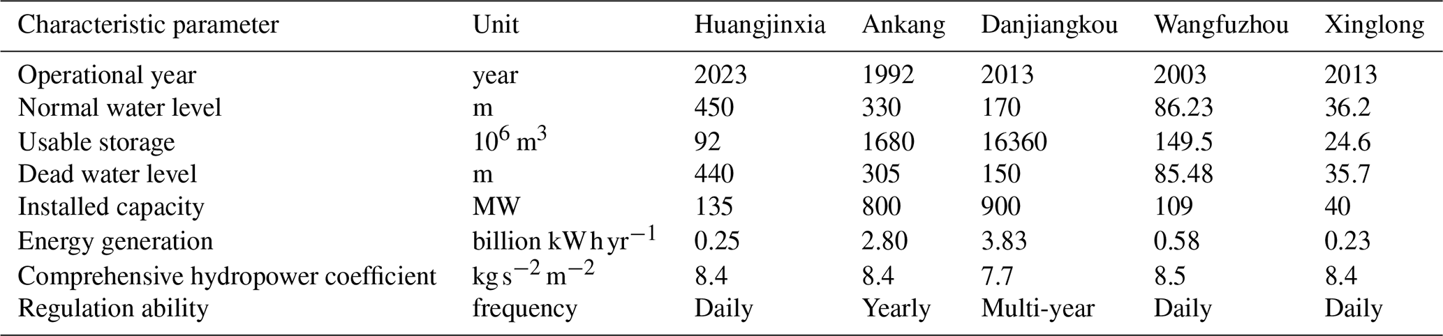
The Hanjiang River, as the largest tributary of the Changjiang River, plays an important role in China's economic development and ecological environment (Xia et al., 2020). The Hanjiang River originates from the Qinling Mountains and traverses Shaanxi, Hubei, and Henan before joining the Changjiang River in Wuhan. The Hanjiang River Basin (HRB) has a basin area of about 159 000 km² and has different clusters of IWDPs (Stone and Jia, 2006). In this study, we choose the Han-to-Wei Water Diversion Project (Wei et al., 2020), the middle route of the South-to-North Water Diversion Project (Li et al., 2016), and the Northern Hubei Water Resources Allocation Project (He and X, 2020) to analyze the water donation impacts of IWDPs on the SHE nexus. The Three Gorges Reservoir to Hanjiang River (Yang et al., 2012) and the Changjiang-to-Han River Water Diversion Project (Zhang et al., 2022) are selected to discuss the water receiving impacts in HRB. For all IWDPs, the scheduling rules for donation and receiving are followed. The HRB hosts numerous reservoirs, with a cascade of 15 reservoirs along its mainstream, starting with the Huangjinxia Reservoir. These reservoirs play significant roles in flood control, water supply, hydropower generation, and ecological conservation (Liu et al., 2018). The Huangjinxia Reservoir (HJX), Ankang Reservoir (AK), Danjiangkou Reservoir (DJK), Wangfuzhou Reservoir (WFZ), and Xinglong Reservoir (XL) are chosen as research nodes, due to their extensive spatial distribution and different priority orders of S, H, and E. Among them, HJX, DJK, and XL are water-supply-prioritized reservoirs, while AK and WFZ are hydropower-generation-prioritized reservoirs. An overview map of HRB and a sketch graphic are shown in Figs. 4 and 5. The characteristic parameter values of the reservoirs are listed in Table 3.

3.2 Data sources

Based on the availability of observed runoff data and water supply volume data in the HRB, the period 1972–2020 is chosen for runoff simulation, and the scenario simulation period is selected as 2006–2020. Observed runoff data were obtained from the Hydrology Bureau of the Changjiang Water Resources Commission, with monthly runoff data selected from six hydrological stations: Xiangjiaping, Baihe, Huanglongtan, Huangjiagang, Xiangyang, and Huangzhuang. Meteorological forcing data for the HRB were sourced from the National Meteorological Science Data Center (http://data.cma.cn/, last access: 5 August 2023). A total of 88 meteorological stations were selected for daily precipitation, maximum and minimum temperatures, and average wind speeds from 1972 to 2020. These data were interpolated onto a 5 arcmin orthogonal grid using the inverse distance weighting method. Digital elevation model (DEM) data, with a spatial resolution of 90 m, were provided by the Geospatial Data Cloud website (http://www.gscloud.cn/, last access: 10 August 2023). Vegetation parameter data were sourced from the global vegetation cover classification database with 1 km resolution developed by the University of Maryland (Hansen et al., 1998). Soil parameter data were sourced from the Cold and Arid Regions Science Data Center (https://www.ncdc.ac.cn/portal/, last access: 10 August 2023), utilizing the Harmonized World Soil Database (HWSD) created by the Food and Agriculture Organization (FAO) and the International Institute for Applied Systems Analysis (IIASA), at 5 arcmin resolution. The relevant physical parameters of soils, divided into 14 types, including bare soil, were estimated using the Soil Water Characteristics (SWCT) module in SPAW software. Reservoir characteristic parameters were primarily sourced from the official websites, reservoir design reports, and related literature. The water supply volume data were obtained from the water resources bulletins of cities in HRB from 2006 to 2020. Based on the water supply data from administrative regions, the water supply volume for the study area is calculated through ArcGIS.

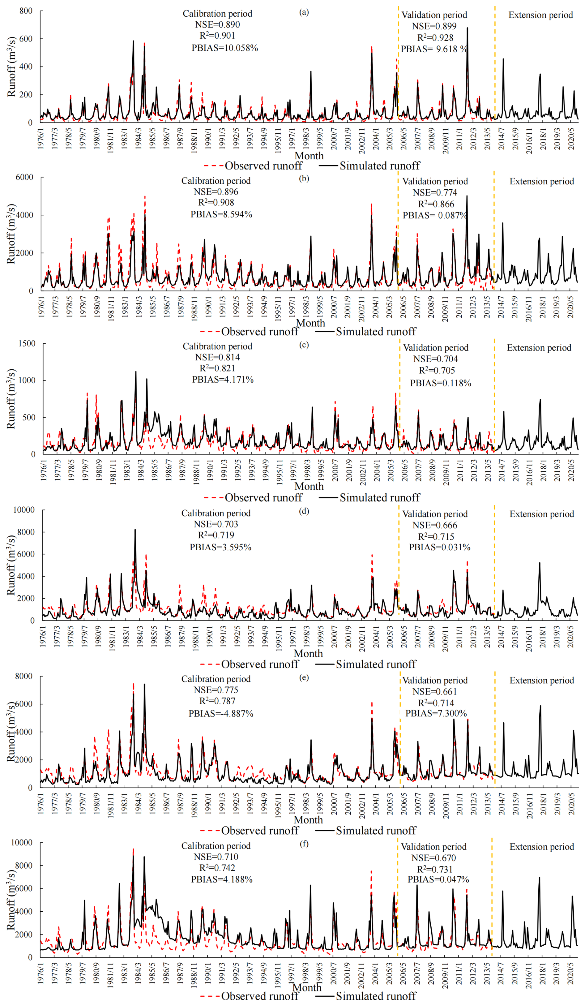
Figure 6 Calibration and validation results of simulation at hydrological stations: (a) Xiangjiangping, (b) Baihe, (c) Huanglongtan, (d) Huangjiagang, (e) Xiangyang, (f) Huangzhuang.

4 Results

4.1 Calibration and verification of VIC model

The HRB was discretized into 2103 grids of 5 arcmin. Inputting meteorological forcing, soil parameters, and vegetation parameter data for each grid, runoff was simulated. The model warm-up period was 1972–1975, with calibration from 1976 to 2005 and validation from 2006 to 2013, while runoff from 2014 to 2020 was simulated for post-validation. All these results are shown in Fig. 6. It can be found that the accuracies of the simulations at all hydrological stations are acceptable and that superior performances were found in the upstream part of the HRB. For instance, NSEs for calibration and validation were 0.90 and 0.77, with corresponding R² of 0.91 and 0.87 at Baihe (BH). Due to the intense human activity impacts in mid–lower reaches of the HRB, the performance was poorer at Huangjiagang (HJG), although the NSEs still exceeded 0.60; PBIAS for all these six stations during calibration and validation periods ranged within [−5 %, 11 %], indicating satisfactory agreement.

Table 4 Multi-level ecological flows resulting from the MTMMHC method.

4.2 Multi-level ecological flow classification and calculation results

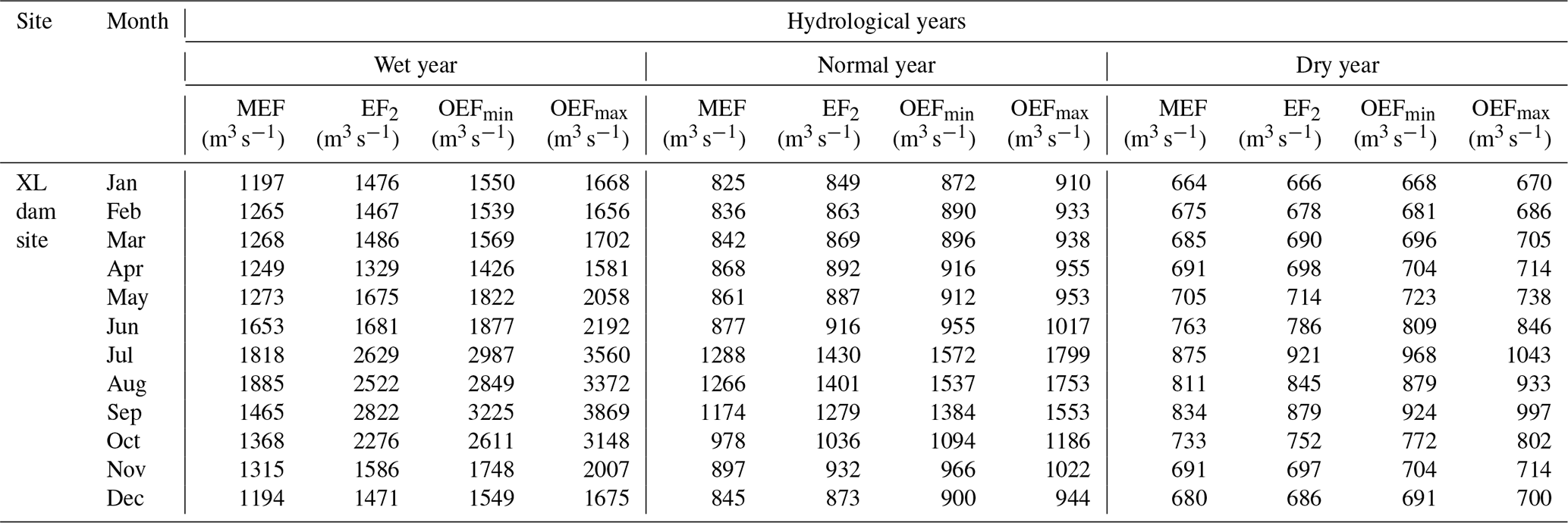
The multi-level ecological flows at the HJX, AK, DJK, WFZ, and XL reservoir dam sites for each month were determined through the MTMMHC method. The EFs are categorized in four levels: MEF, EF₂, OEF_min, and OEF_max. The results at the XL reservoir dam site from the MTMMHC method are presented in Table 4. The EFs for wet, normal, and dry years show decreasing trends, with higher values during the flood season. The peak ecological flow occurs in August during wet years but in July during both normal and dry years. All the peak EFs for the other four sites occur between July and September. The peak EFs for the HJX and AK reservoir dam sites during wet, normal, and dry years occur in July or August. The peak values for DJK and WFZ are dispersed and are found in September, August, and July. The EFs at the five reservoir dam sites are significantly higher from June to September than in other months. The EFs for wet, normal, and dry years are similar to related ecological flow quantification results in the HRB (Zhang, et al., 2022, Li and Kang, 2014).

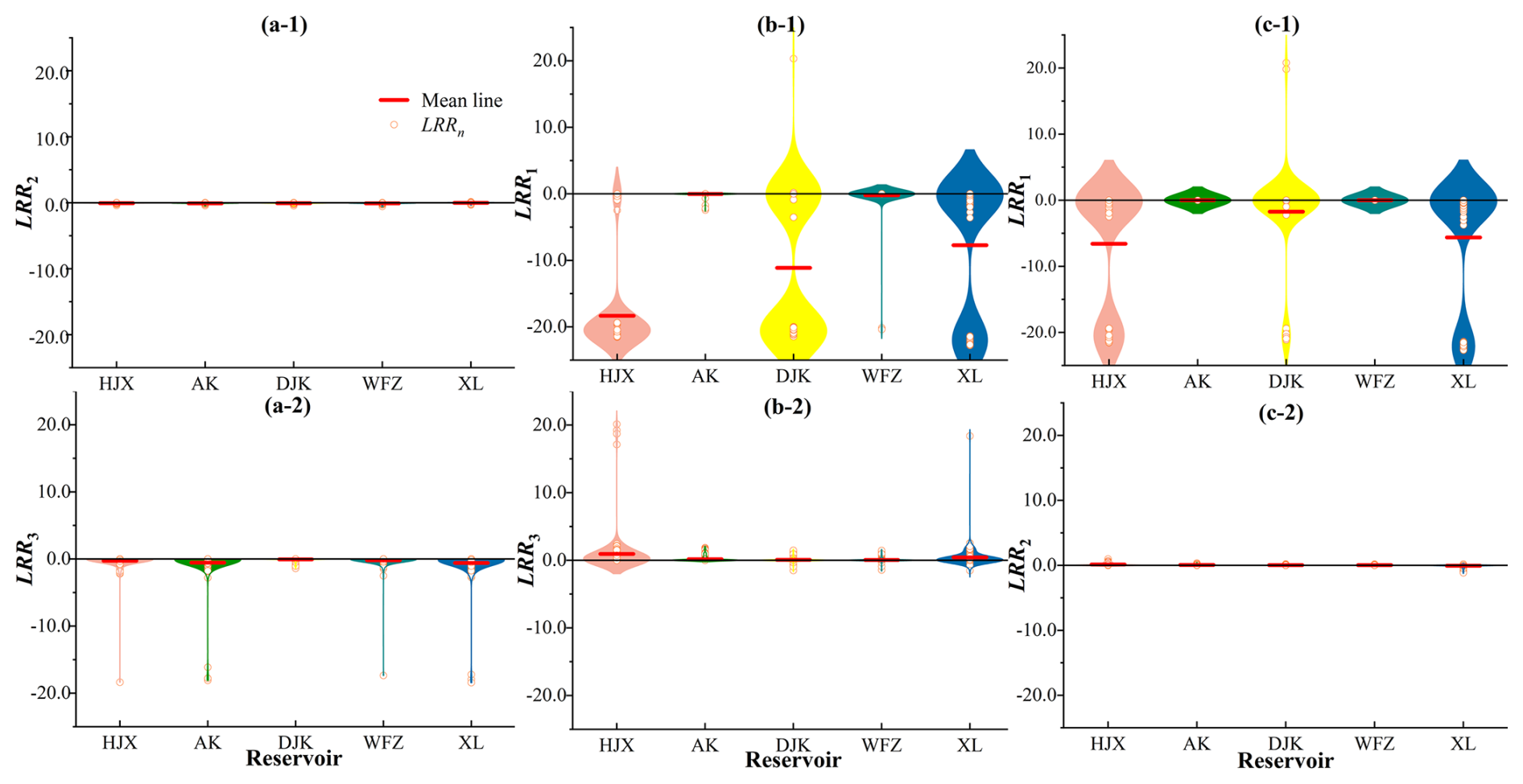
Figure 7 Differences of indexes (i.e., LRR₁, LRR₂, LRR₃ for log response ratios of the S, H, and E components) without IWDPs (i.e., between S_0-p-n and S_0-4-n) at the monthly scale: (a-1) LRR₂ with the highest priority in S (i.e., between S_0-1-2 and S_0-4-2), (a-2) LRR₃ with the highest priority in S (i.e., between S_0-1-3 and S_0-4-3), (b-1) LRR₁ with the highest priority in H (i.e., between S_0-2-1 and S_0-4-1), (b-2) LRR₃ with the highest priority in H (i.e., between S_0-2-3 and S_0-4-3), (c-1) LRR₁ with the highest priority in E (i.e., between S_0-3-1 and S_0-4-1), (c-2) LRR₂ with the highest priority in E (i.e., between S_0-3-2 and S_0-4-2).

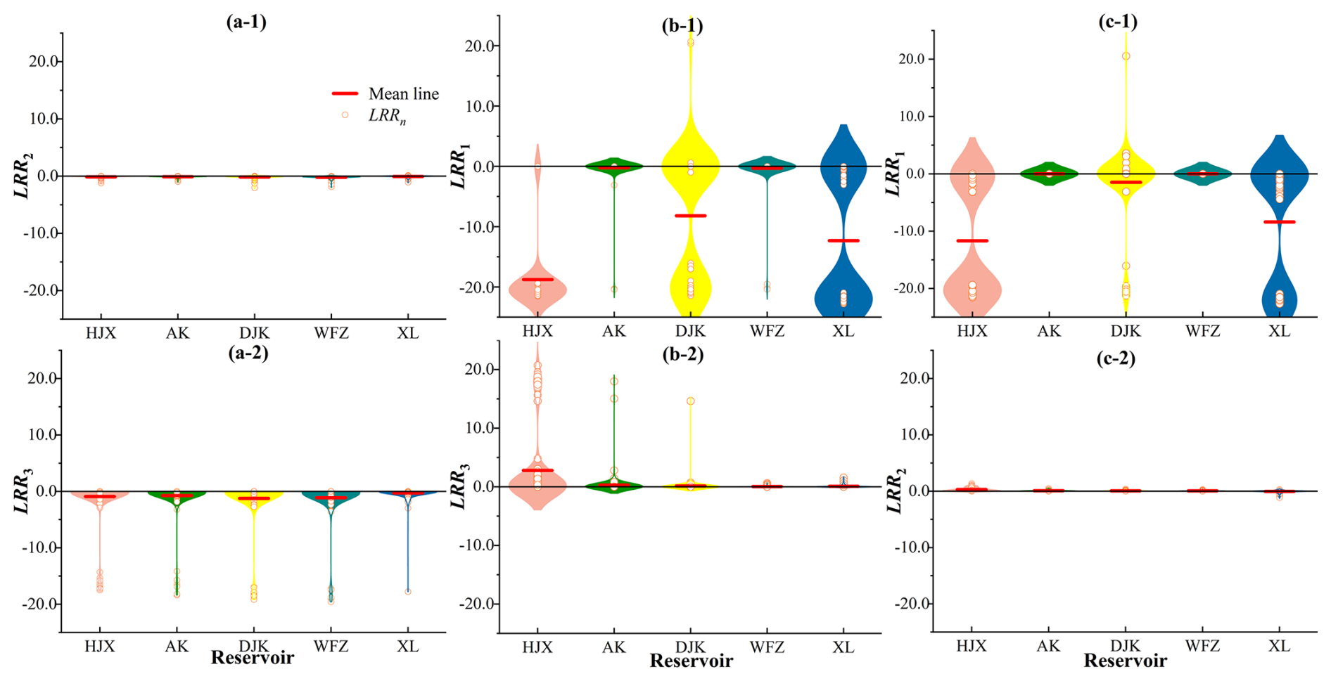
Figure 8 Differences of indexes (i.e., LRR₁, LRR₂, LRR₃ for log response ratios of the S, H, and E components) with IWDPs (i.e., between S_3-p-n and S_3-4-n) at the monthly scale: (a-1) LRR₂ with the highest priority in S (i.e., between S_3-1-2 and S_3-4-2), (a-2) LRR₃ with the highest priority in S (i.e., between S_3-1-3 and S_3-4-3), (b-1) LRR₁ with the highest priority in H (i.e., between S_3-2-1 and S_3-4-1), (b-2) LRR₃ with the highest priority in H (i.e., between S_3-2-3 and S_3-4-3), (c-1) LRR₁ with the highest priority in E (i.e., between S_3-3-1 and S_3-4-1), (c-2) LRR₂ with the highest priority in E (i.e., between S_3-3-2 and S_3-4-2).

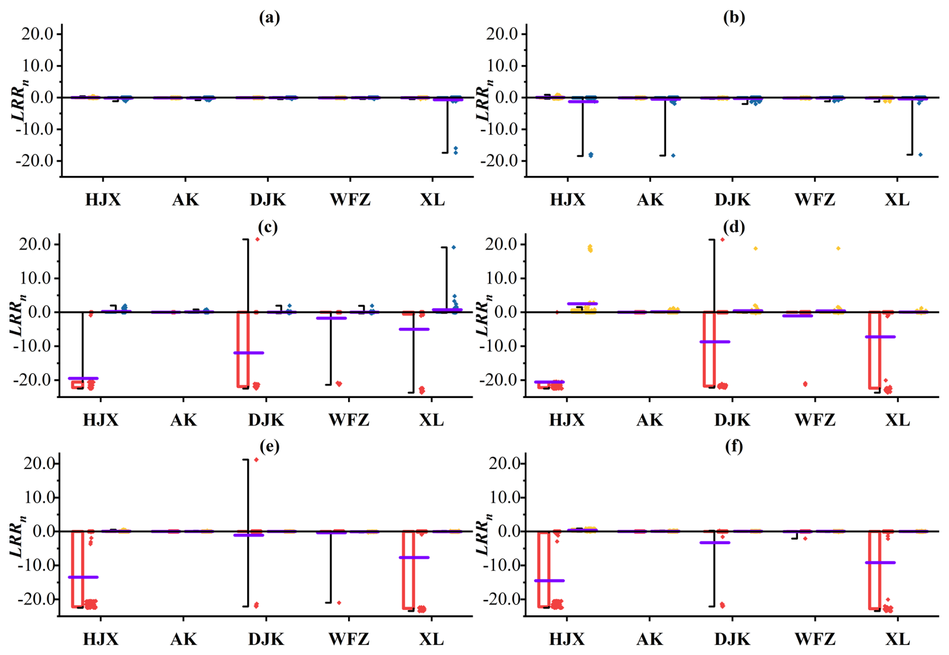
Figure 9 LRR_n with different highest priorities (i.e., between S_m-1-n and S_m-4-n) at the seasonal scale: (a, b) LRR_n with the highest priority in S without IWDPs (i.e., between S_0-1-n and S_0-4-n) and with IWDPs (i.e., between S_3-1-n and S_3-4-n), (c, d) LRR_n with the highest priority in H without IWDPs (i.e., between S_0-2-n and S_0-4-n) and with IWDPs (i.e., between S_3-2-c and S_3-4-n). (e, f) LRR_n with the highest priority in E without IWDPs (i.e., between S_0-3-n and S_0-4-n) and with IWDPs (i.e., between S_3-3-n and S_3-4-n).

4.3 Responses of indexes in feedback loops with different clusters of IWDPs in a reservoir group

4.3.1 Responses of indexes in feedback loops without and with IWDPs

To analyze the feedback loops of SHE nexus without IWDPs (i.e., S_0-p-n and S_0-4-n) and with IWDPs (i.e., S_3-p-n and S_3-4-n) across the multiple temporal (i.e., monthly, seasonal, and annual) and spatial (i.e., five reservoirs) scales, the differences in indexes (i.e., LRR₁, LRR₂, LRR₃ for the log response ratios of the S, H, and E components) between S_0-p-n and S_0-4-n or between S_3-p-n and S_3-4-n are determined at the different time scales in a reservoir group. Monthly differences are presented in Figs. 7 and 8, while the seasonal results are shown in Fig. 9. Corresponding annual-scale results can be found in Tables S1 and S2 in the Supplement.

If there are no IWDPs and S-priority is set, the mean values of both LRR₂ and LRR₃ in five reservoirs remain below 0, as shown in Fig. 7a. As there are a large number of negative values of LRR₂ in all reservoirs with S-priority, as shown in Fig. 7a-1, the hydropower generation is found to be reduced in most months. However, there are still some positive values of LRR₂ in reservoirs. XL reservoir shows a higher occurrence of positive values of LRR₂ when there is abundant water, such as in July 2007 and September 2017. As shown in Fig. 7a-2, all five reservoirs exhibit a negative LRR₃ in all months. The value of LRR₃ for DJK reservoir is closest to 0. The smallest mean values of LRR₃ for XL and AK reservoirs are −0.61 and −0.54, respectively. The reduction of ecological flow satisfaction rates for DJK is smaller than that for other reservoirs due to its effective regulation. The values of ecological flow satisfaction rates for XL and AK decrease significantly, due to the greater reductions of ecological flow and the higher ecological flow standards at these two reservoir dam sites. The extreme values (e.g., lower than 90 % months values) of LRR₃ for HJX, AK, WFZ, and XL reservoirs occur in the higher water supply demand months, such as June to September of each year. There are also differences between the results of LRR₂ and LRR₃; the range of LRR₃ is wider, while that of LRR₂ is relatively concentrated and closer to 0.

If there are no IWDPs and H-priority is set, the values of LRR₁ for all five reservoirs are less than 0 in most months, and the mean values of LRR₃ exceed 0, as shown in Fig. 7b. The water supply for HJX, DJK, and XL is significantly decreased, while the water supply for AK and WFZ has slight reductions, as shown in Fig. 7b-1. There are two positive values of LRR₁ for DJK reservoir, occurring in January 2010 and July 2011. In January 2010, higher water storage resulting from H-priority increases water availability. With H-priority, reservoirs with regulating capacity will store more water, leading to increased generation flow during dry periods (Zhang et al., 2014), while, as in July 2011, an increase in the discharge flow from the upstream reservoir increases the water supply. As shown in Fig. 7b-2, the values of ecological flow satisfaction rates for HJX reservoir significantly increase. DJK and its downstream reservoirs have negative values of LRR₃ in abundant-water months because of the increased storage capacity and the reduced inflow into DJK. The water resource allocation of DJK affects the SHE system of downstream reservoirs. There are also differences between the results for LRR₁ and LRR₃; the values of LRR₃ are relatively closer to 0 than those of LRR₁. The feedback loops on S are more pronounced than on E. The extreme values of LRR₁ and LRR₃ are always found in months with small water flow in the river but with high water supply demand.

If there is no IWDP and E-priority is set, the mean values of LRR₁ for HJX, DJK, and XL reservoirs are negative, as shown in Fig. 7c-1. However, the values of LRR₁ for AK and WFZ are almost 0 because their increased discharge water from upstream is prioritized for release for hydropower generation, and no excess is for water supply. Thus, prioritizing E has less impact on S for reservoirs, due to the main function of hydropower generation. DJK and XL exhibit some positive values of LRR₁ because of increased inflows from upstream. Therefore, the increased inflow to upstream reservoirs alleviates the negative feedback loops of E on S in downstream reservoirs. As shown in Fig. 7c-2, the mean values of LRR₂ for HJX, AK, DJK, and WFZ reservoirs are positive but close to 0. While XL has a small negative mean value of LRR₂, it experiences greater decreases in hydropower generation, primarily due to its smaller installed capacity (Zhang, 2008). Negative values of LRR₂ can be found in abundant-water months. The ranges of LRR₁ and LRR₂ are also different. The former is wide while the latter is narrow and its values are closer to 0.

The differences between scenarios S_3-p-n and S_3-4-n were determined to analyze the feedback loops with IWDPs, as shown in Fig. 8a–c. It can be found that the positive or negative signs of the LRR_n values with IWDPs are consistent with those without IWDPs. If there are IWDPs and S-priority is set, the mean value of LRR₃ for XL shows an increase, while all the values of LRR₂ and LRR₃ for the other four reservoirs are lower than those without IWDPs, as shown in Figs. 8a and 7a. The mean values of LRR₂ with IWDPs for the five reservoirs are all negative but small and the mean values of LRR₃ are slightly more negative. DJK reservoir gets more extreme values, due to the impacts of IWDPs. The values of LRR₂ with IWDPs are lower than −0.45 (i.e., the minimum value of LRR₂ without IWDPs) in 6 % of the months, while the values of LRR₃ are lower than −1.40 (i.e., the minimum value of LRR₃ without IWDPs) in 8 % of the months. It is evident that IWDPs strengthen the negative feedback loops of the S component on the other two components in HJX, AK, DJK, and WFZ, while IWDPs weaken negative feedback loops of S on E for XL. As shown in Fig. 8b-1, if there are IWDPs and H-priority is set, the mean values of LRR₁ for HJX, AK, and XL reservoirs decrease significantly but the mean value of LRR₁ for DJK reservoir increases due to IWDPs. The differences in water supply between the S_3-2-n and S_3-4-n scenarios remain negligible despite further reductions in water supply with H-priority. As shown in Fig. 8b-2, the values of LRR₃ for HJX, AK, DJK, and WFZ increase further than those in Fig. 7b-2 without IWDPs. The values of LRR₃ for XL decrease slightly, due to the positive feedback loops of the H component on E and the IWDP impacts. As shown in Fig. 8c-1, if there are IWDPs and E-priority is set, the mean values of LRR₁ for HJX and XL decrease. The mean values of LRR₁ for AK and WFZ remain at almost 0, while the mean value of LRR₁ for DJK increases with IWDPs compared with without IWDPs. As shown in Fig. 8c-2, the mean values of LRR₂ for five reservoirs increase slightly with IWDPs, compared with without IWDPs. The positive feedback loops of the E component on H are strengthened, while the negative feedback loops are weakened.

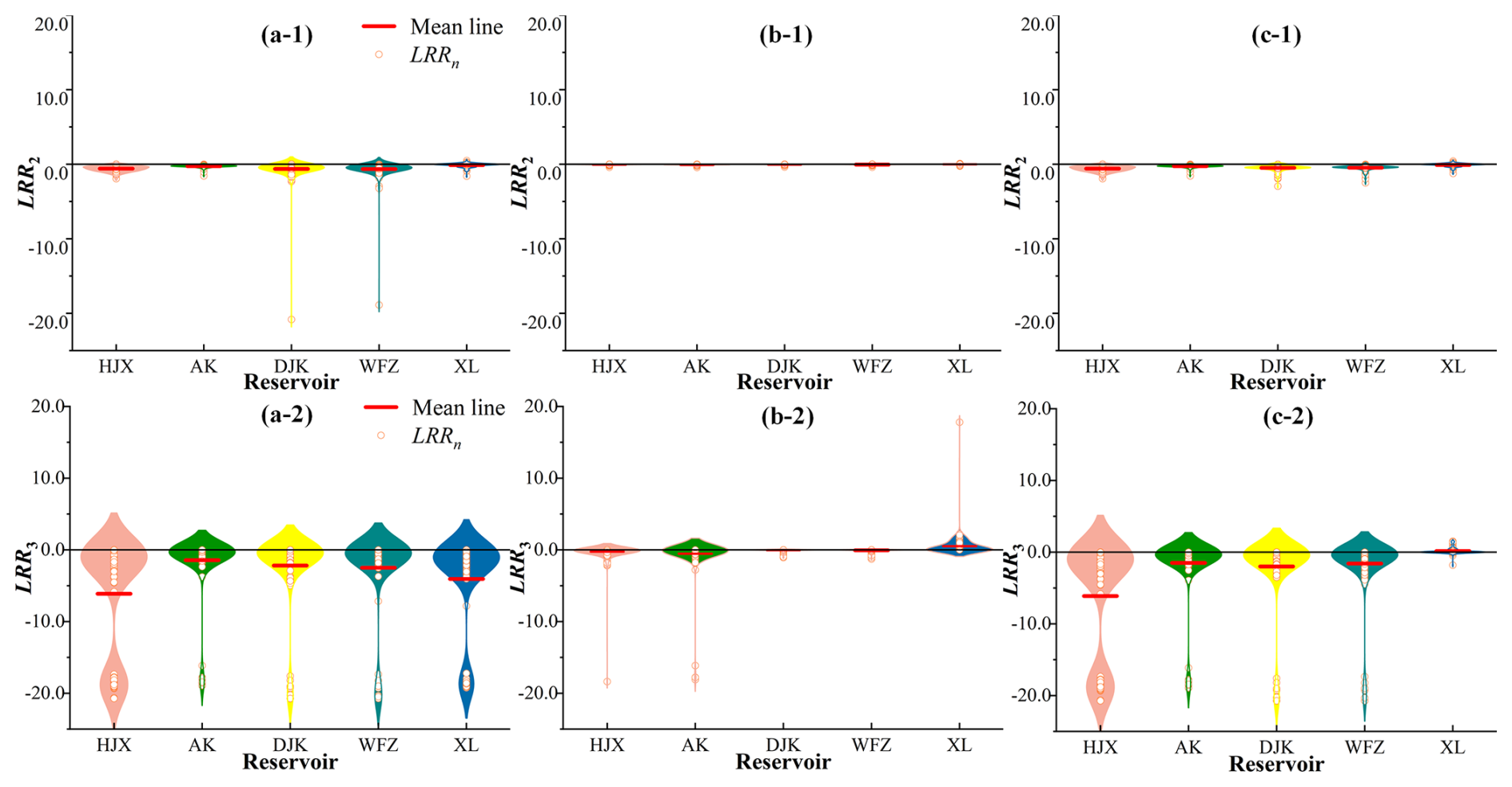
Figure 10 LRR_n values when there are different clusters of IWDPs and S-priority is set at the monthly scale: (a-1, a-2) LRR₂ and LRR₃ when there is only water donation (i.e., between S_1-1-n and S_0-4-n), (b-1, b-2) LRR₂ and LRR₃ when there is only water receiving (i.e., between S_2-1-n and S_0-4-n), (c-1, c-2) LRR₂ and LRR₃ when there are both donation and receiving (i.e., between S_3-1-n and S_0-4-n).

In this study, March, April, and May are taken as spring; June, July, and August are taken as summer; September, October, and November are taken as autumn; and December and January and February of the following year are taken as winter. The values of LRR_n for the five reservoirs at the seasonal scale are shown in Fig. 9. If there is no IWDP but S-priority is still set, positive values of LRR₂ for HJX and XL are found in summer, while all negative values of LRR₂ for the other three reservoirs are found in all seasons, as shown in Fig. 9a. All values of LRR₃ for the five reservoirs are negative in all seasons. If there are IWDPs and S-priority is set, the mean value of LRR₃ for XL increases, while the values of LRR₂ and LRR₃ for the other four reservoirs are less than those without IWDPs, as shown in Fig. 9b. These negative values indicate that IWDPs significantly strengthen the negative feedback loops of the S component on H and E in reservoirs and weaken negative feedback of S on E in XL. If there are no IWDPs but H-priority is set, negative values of LRR₁ and positive values of LRR₃ are found for the five reservoirs, as shown in Fig. 9c. For HJX, DJK, and XL reservoirs, negative values of LRR₁ are found in winter, while zero values of LRR₁ are found in summer. The mean values of LRR₁ are close to 0 in AK and WFZ reservoirs in all seasons. Positive values of LRR₃ are smaller in HJX, AK, DJK, and WFZ reservoirs, while those in XL are greater in winter with a low flow. If there are IWDPs and H-priority is set, the values of LRR₁ for all reservoirs are lower than those without IWDPs, as shown in Fig. 9d. Values of LRR₃ for HJX, AK, DJK, and WFZ reservoirs are greater than those without IWDPs, while those for XL are close to 0. If there are no IWDPs and E-priority is set, negative values of LRR₁ for HJX, DJK, WFZ, and XL reservoirs can be found in almost every season, while zero values of LRR₁ for AK reservoir can be found in all seasons. As shown in Fig. 9e, two positive values of LRR₁ for DJK are found, in spring and winter of 2007, due to the increased discharge water from AK reservoir. The positive values of LRR₂ for the five reservoirs are found in most seasons, but a few negative values are found in summer. If there are IWDPs and E-priority is set, more positive values of LRR₂ for the five reservoirs and less negative values of LRR₁ are found in HJX, DJK, WFZ, and XL reservoirs.

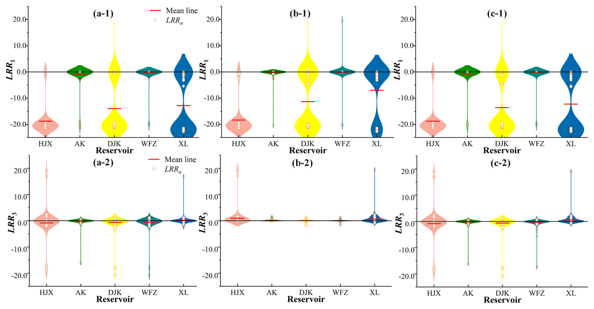
Figure 11 LRR_n values when there are different clusters of IWDPs and H-priority is set at the monthly scale: (a-1, a-2) LRR₂ and LRR₃ when there is only water donation (i.e., between S_1-2-n and S_0-4-n), (b-1, b-2) LRR₂ and LRR₃ when there is only water receiving (i.e., between S_2-2-n and S_0-4-n), (c-1, c-2) LRR₂ and LRR₃ when there are both donation and receiving (i.e., between S_3-2-n and S_0-4-n).

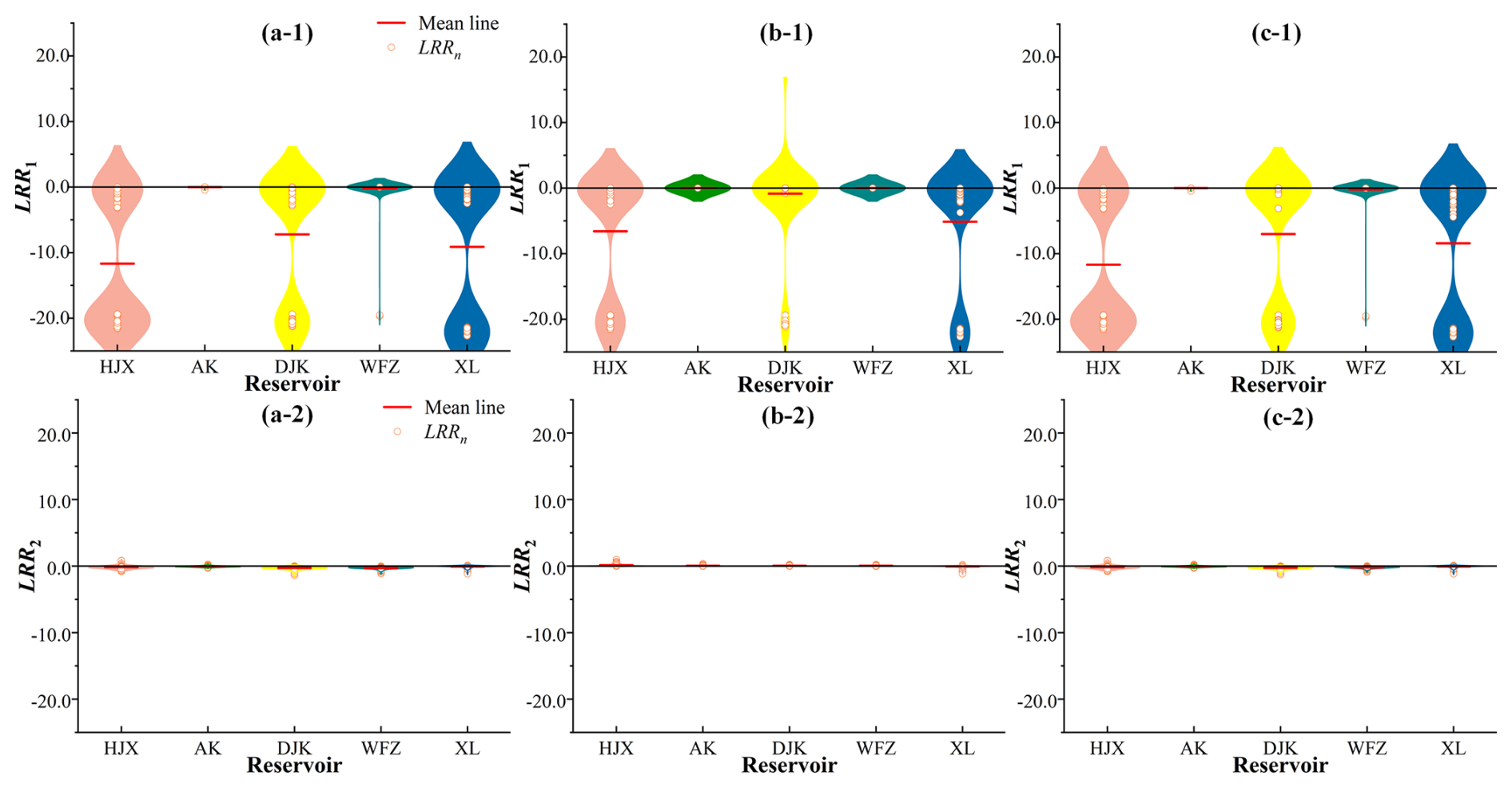
Figure 12 LRR_n values when there are different clusters of IWDPs and E-priority is set at the monthly scale: (a-1, a-2) LRR₁ and LRR₂ when there is only water donation (i.e., between S_1-3-n and S_0-4-n), (b-1, b-2) LRR₁ and LRR₂ when there is only water receiving (i.e., between S_2-3-n and S_0-4-n), (c-1, c-2) LRR₁ and LRR₂ when there are both donation and receiving (i.e., between S_3-3-n and S_0-4-n).

Figure 13 LRR_n values when there are different clusters of IWDPs at the seasonal scale: (a-1, a-2, a-3) LRR_n when there is only water donation, when there is only water receiving, when there are both donation and receiving and S-priority is set (i.e., between S_m-1-n and S_0-4-n); (b-1, b-2, b-3) the same when H-priority is set (i.e., between S_m-2-n and S_0-4-n); (c-1, c-2, c-3) the same when E-priority is set (i.e., between S_m-3-n and S_0-4-n).

4.3.2 Responses of indexes in feedback loops with only water donation, only water receiving, and both donation and receiving

To analyze the impacts of only water donation (i.e., S_1-p-n and S_0-4-n), only water receiving (i.e., S_2-p-n and S_0-4-n), and both donation and receiving (i.e., S_3-p-n and S_0-4-n) on feedback loops of SHE nexus across the multiple temporal and spatial scales, the differences of indexes between S_m-p-n and S_0-4-n are determined in a reservoir group. The results of the monthly differences are shown in Figs. 10–12. The seasonal results are shown in Fig. 13. Corresponding annual-scale results can be found in Tables S3–S5 in the Supplement.

If there is only water donation and S-priority is set, values of LRR₂ and LRR₃ for the five reservoirs are negative and lower than those without IWDPs, as shown in Fig. 10a-1 and a-2; water donation strengthens the negative feedback of S on H and E for the five reservoirs. More small negative values are found in DJK. If there is only water receiving and S-priority is set, values of LRR₂ and LRR₃ for HJX and AK are the same as those without IWDPs. Meanwhile, for DJK, WFZ, and XL, the values are close to 0. XL exhibits a lot of positive values of LRR₃, as shown in Fig. 10b-1 and b-2. If there are both water donation and receiving, the mean values of LRR₂ for the five reservoirs are all negative, and the mean values of LRR₃ for the five reservoirs are also negative, except XL, as shown in Fig. 10c-1 and c-2. IWDPs strengthen the negative feedback loops of S on H and E for HJX, AK, DJK, and WFZ and weaken the negative feedback loops of S on E for XL.

If there is only water donation and H-priority is set, values of LRR₁ and LRR₃ for the five reservoirs are lower than those without IWDPs, as shown in Fig. 11a-1 and a-2. Negative values of LRR₃ for the five reservoirs are found in low-flow months, such as November, December, and January. Thus, water donation is found to strengthen the feedback loops of H on S and E, especially in low-flow months. If there is only water receiving and H-priority is set, values of LRR₁ and LRR₃ for DJK, WFZ, and XL are greater than those without IWDPs, as shown in Fig. 11b-1 and b-2. Water receiving weakens the feedback loops of H on S and E. If there are both water donation and receiving and H-priority is set, the mean values of LRR₁ and LRR₃ for DJK, WFZ, and XL are still lower than those without IWDPs and the mean value of LRR₃ for XL is greater than those without IWDPs, as shown in Fig. 11c-1 and c-2.

If there is only water donation and E-priority is set, then values of LRR₁ and LRR₂ for the five reservoirs are as shown in Fig. 12a-1 and a-2. The mean values of LRR₁ and LRR₂ for these five reservoirs are all negative, and all these values are lower than those without IWDPs. Unlike the values of LRR_n without IWDPs, there are no positive values of LRR₁ for DJK and few positive values of LRR₂ for the five reservoirs, due to the decreased inflows from upstream with water donation. If there is only water receiving and E-priority is set, values of LRR₁ and LRR₂ for DJK, WFZ, and XL are greater than those without IWDPs. If there are both water donation and receiving and E-priority is set, the mean values of LRR₁ and LRR₂ for DJK, WFZ, and XL are still lower than those without IWDPs, as shown in Fig. 12c-1 and c-2.

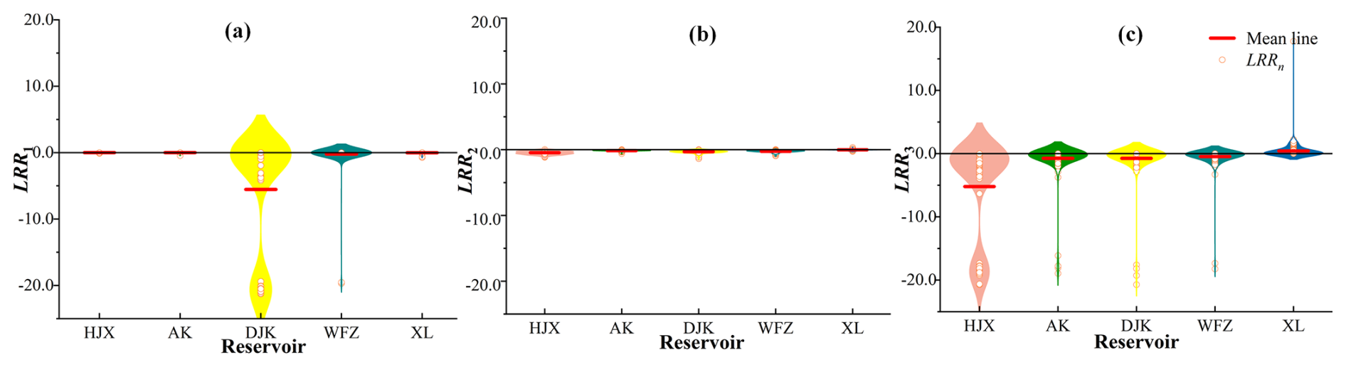
Figure 14 Differences of indexes (i.e., (a) LRR₁, (b) LRR₂, (c) LRR₃ for log response ratio of the S, H, and E components) between S_3-4-n and S_0-4-n at the monthly scale.

If there is only water donation and S-priority is set, values of LRR₂ and LRR₃, as shown in Fig. 13a-1, are lower than those without IWDPs in all seasons, as shown in Fig. 9a. If there is only water receiving and S-priority is set, mean values of LRR₂ and LRR₃ for DJK, WFZ, and XL, as shown in Fig. 13a-2, are all greater than those without IWDPs. If there are both water donation and receiving and S-priority is set, mean values of LRR₂ for the five reservoirs decrease, compared with those without IWDPs. Mean values of LRR₃ for HJX, AK, DJK, and WFZ decrease but those for XL increase, compared with those without IWDPs, as shown in Fig. 13a-3. If there is only water donation and H-priority is set, values of LRR₁ and LRR₃, as shown in Fig. 13b-1, are lower than those without IWDPs. Water donation strengthens feedback loops of H on S for HJX, DJK, and XL. If there is only water receiving and H-priority is set, mean values of LRR₂ for DJK, WFZ, and XL increase, while mean values of LRR₃ for DJK, WFZ, and XL only increase slightly, compared with those without IWDPs. If there are both water donation and receiving and H-priority is set, mean values of LRR₂ for the five reservoirs are negative or 0 (AK), and mean values of LRR₃ for the reservoirs except XL are close to 0, as shown in Fig. 13b-3. If there is only water donation and E-priority is set, it can be found that values of LRR₁ and LRR₂ in all seasons are lower than those without IWDPs, as shown in Fig. 13c-1. Mean values of LRR₁ and LRR₂ for the five reservoirs all decrease. If there is only water receiving and E-priority is set, mean values of LRR₁ and LRR₂ for DJK and WFZ and mean values of LRR₁ for XL are greater than those without IWDPs, while mean values of LRR₂ for XL increase, as shown in Fig. 13c-2. If there are both water donation and receiving and E-priority is set, values of LRR₁ and LRR₂ for DJK and WFZ and values of LRR₁ for XL, as shown in Fig. 13c-3, are greater than those with only water donation, while lower than those without IWDPs, while values of LRR₂ for XL are greater than those without IWDPs because of the reduced spilled water. Therefore, values of LRR_n at the seasonal scale demonstrate a consistent conclusion with those at the monthly scale. Moreover, the values of LRR_n are relatively stable in summer, while they change greatly in winter at seasonal scale. The impacts of IWDPs on SHE nexus are more significant in low-flow seasons.

4.4 Responses of the three components with IWDPs

To identify the impacts of IWDPs on S, H, and E components in a reservoir group, differences between indexes without IWDPs and with IWDPs (i.e., S_3-4-n and S_0-4-n) were determined. Negative values of LRR₁ for the five reservoirs are found in all months, as shown in Fig. 14a. It is found that values of LRR₁ for DJK are significantly smaller than those for the other reservoirs. Mean values of LRR₂ for the five reservoirs are all negative, as shown in Fig. 14b. Positive values of LRR₃ are found in XL and negative values of LRR₃ are found in HJX, AK, DJK, and WFZ in all months, as shown in Fig. 14c.

5 Discussion

The proposed framework reveals significant negative feedback loops of the water supply (S) on both hydropower generation (H) and environment conservation (E), as evidenced by reductions in hydropower generation (negative LRR₂ in Fig. 7a-1) and ecological flow satisfaction rate (negative LRR₂ in Fig. 7a-2) with S-priority. The negative feedback loops of the S component on E are more pronounced than those on H, as evidenced by the wider range of variation in LRR₃ values compared with LRR₂ values. These findings are consistent with previous studies on SHE nexus (Chen et al., 2018; Khalkhali et al., 2018). It has been found that there are a few positive feedback loops between S and H in abundant-water months because the increased spilled water leads to a reduction in hydropower generation (Jiang et al., 2018). Thus, the increasing water storage or increasing water supply can still ensure hydropower generation. The values of ecological flow satisfaction rates for XL and AK significantly decrease, due to the greater reductions of ecological flow and the higher ecological flow standards at the two reservoir dam sites. The extreme values (e.g., lower than 90 % months values) of LRR₃ for HJX, AK, WFZ, and XL reservoirs occur in the higher water supply demand months, such as June to September of each year. And Gao et al. (2023) find that the higher the water supply demand, the lower the ecological flow left in rivers. The environment conservation of downstream river systems is critically influenced by upstream water supply decisions (Gupta, 2008). Contrary to the unidirectional positive nexus between hydropower generation and environment conservation proposed by Wei et al. (2022), our study reveals bidirectional feedback loops of H and E, aligning with Wu et al. (2023). The positive feedback loops between H and E are weakened or even become negative in small installed capacity hydropower generation reservoirs (e.g., the XL reservoir, Zhang et al., 2008), in abundant-water months particularly. The increased flows for hydropower generation alleviate the pressure of ecological damage in rivers. However, the more flows for hydropower generation there are from the reservoir, the less water resources for supply (Doummar et al., 2009) are available, leading to negative impacts on the S component. The feedback loops of H on S are more pronounced than on E, as shown by the wider range of variation in LRR₁ values compared with LRR₃ values. Negative feedback of the E component on S for reservoirs has been found when the main function is water supply, while no significant effect on reservoirs has been found when the main function is hydropower generation (negative LRR₁ in Fig. 7c-1). There are both negative and positive feedback loops of the E component on H, while the negative feedback loops strengthen in abundant-water months. Feedback loops of the E component on S are stronger than those on H, as shown by the values of LRR_n. The negative feedback loops between S and H, and between S and E, are strong in low-flow months, due to the high water supply demand. Stronger competition for water among S, H, and E occurs in low-flow months, with stronger negative feedback loops of the SHE nexus (Wu et al., 2023). Feedback loops of SHE nexus in reservoirs with regulation functions (e.g., AK and DJK) remain stable under the varying inflow conditions. These reservoirs reasonably allocate water among S, H, and E components to prevent strengthening of negative feedback loops in low-flow months. Furthermore, increasing hydropower generation flow might have impacts on downstream water quality and biodiversity (Botelho et al., 2017; Martinez et al., 2019); the feedback loops of H on E are enhanced.

Inter-basin water diversion projects (IWDPs) have negative impacts on the regional water supply from DJK and upstream reservoirs with negative LRR₁, consistent with Hong et al. (2016) and Ouyang et al. (2018). All reservoirs experience reduced hydropower generation, but there are positive impacts on H in abundant-water months (positive LRR₂ in Fig. 14b). Many studies have highlighted the negative impacts of IWDPs on hydropower generation (Yang, et al., 2023) but the positive impacts are less frequently discussed. With the water donation for the Han-to-Wei Water Diversion Project, the middle route of the South-to-North Water Diversion Project and the Northern Hubei Water Resources Allocation Project, multiple algal bloom events occurred downstream of the HRB (Tian et al., 2022), water donation having a significant negative impact on the environment conservation of the basin. Water received from the Three Gorges Reservoir to Hanjiang River does not compensate for all these negative impacts, and water receiving from the Changjiang-to-Hanjiang River Water Diversion Project benefits environment conservation for XL. It is evident that IWDPs significantly alter the feedback loops of an SHE nexus by modifying water availability. As IWDPs export or import water to or from an area, the amount of available water changes, and can prompt a redistribution and re-planning of the available water (Li et al., 2014), which can significantly impact feedback loops of SHE nexus (Feng, et al., 2019). Although strong responses occur in feedback loops of SHE nexus, the positive or negative nature of feedback among these components remains stable with impacts of IWDPs. Thus, the redistribution and re-planning of available water cannot alter the competition or synergy among the components of an SHE nexus. It is evident that water donation strengthens the negative feedback loops between S and H, the negative feedback loops between S and E, and the positive feedback loops between H and E, while receiving water weakens these feedback loops. Water donation results in a reduction of available water (Mok et al., 2015; Wu et al., 2022), leads to lower flow, stronger competition for water among S, H, and E, and stronger feedback loops. Reduced competition among S, H, and E is found in water receiving areas, primarily due to the replenishing available water resources. The persistent feedback polarity with IWDPs suggests that simply increasing water receiving (e.g., via compensation donations like the Three Gorges Reservoir to Hanjiang River) cannot resolve inherent SHE conflicts – instead, adaptive allocation rules that account for these stable feedback patterns are needed.

The consistency in the signs of mean LRR_n values across the seasonal scale, as shown in Figs. 9 and 13, and annual scale, as shown in Tables S1–S5 in the Supplement, with those at the monthly scale indicates an inherent similarity and stability in SHE nexus feedback loops over different temporal resolutions. Compared with the values of LRR_n at the monthly scale, the values at the seasonal scale show stronger periodic variations. Based on the variations in LRR_n and the mathematical implications of LRR₁, LRR₂, and LRR₃, this study found that these periodic variations align closely with the runoff variations, and the temporal and spatial variations in feedback loops are primarily attributed to variations in runoff. The wavelet transform analysis has also been applied to the runoff for the HJX, AK, DJK, WFZ, and XL dam sites. The results are consistent with those for the Hutuo River Basin (Xu et al., 2018), the periodic variations being at the seasonal scale. The LRR_n values at the seasonal scale can help analyze variations in periodic feedback loops. Unlike the monthly or seasonal scales, results at the annual scale reveal the long-term trends and periodic variations in the inter-annual and spatial trends of an SHE nexus from a macro perspective. The impacts of reservoir operation and regulation on SHE nexus can be clearly simulated and observed at the monthly scale, so the immediate changes in the nexus at the monthly scale can provide information for short-term decision-making in reservoirs.

6 Conclusions

A framework is proposed to address the different impacts of IWDPs on dynamic SHE nexus across multiple temporal and spatial scales in reservoir groups with different priority functions and to explore synergies in feedback loops. The HRB was taken as a case study to verify the feasibility and reliability of this framework. Negative feedback loops can be found between S and H and between S and E, while positive feedback loops can be found between H and E, in a reservoir group without IWDPs. The negative feedback loops of S on H and the positive feedback loops of E on H are weakened or even broken in abundant-water periods. All feedback loops are strengthened in low-flow periods, due to heightened competition for water resources. Water donation strengthens the negative feedback loops between S and H, the negative feedback loops between S and E, and the positive feedback loops between H and E, while water receiving weakens these feedback loops. Feedback loops of an SHE nexus exhibit intrinsic similarity and stability across different time scales. The impact of reservoir operation and regulation on an SHE nexus are clearest at the monthly scale. The seasonal scale reveals variations in periodic feedback loops and the annual scale offers inter-annual and spatial trends of an SHE nexus from a macro perspective. Feedback loops in reservoirs with regulation functions (e.g., AK and DJK) remain stable under varying inflow conditions at the monthly scale. The positive feedback loops between H and E are weakened or even become negative in small installed capacity hydropower generation reservoirs (e.g., the XL reservoir), even in abundant-water periods. Feedback loops for downstream reservoirs are influenced by their upstream reservoirs, especially in low-flow periods. In abundant-water periods, the increasing water donation or regional water supply can increase hydropower generation efficiency due to the reduced spilled water. In dry periods, it is necessary to consider the priority order of S, H, and E, and determine a water utilization threshold for each component to maximize the benefits. We find that simply increasing water receiving cannot resolve inherent SHE conflicts because of the persistent feedback polarity with IWDPs. Adaptive allocation rules are needed that account for these stable feedback patterns.

This framework offers a systematic and quantitative approach to examining the spatiotemporal variations of an SHE nexus with external perturbations. It elucidates the existence and nature of synergies among S, H, and E. However, more work should be done to enrich the representation of each component, such as the E component. This component should be enriched by a comprehensive set of water quality indicators. Then more details of the mechanism of the SHE nexus can be elaborated.