the Creative Commons Attribution 4.0 License.
the Creative Commons Attribution 4.0 License.
 | 25 Jul 2025
Merits and limits of SWAT-GL: application in contrasting glaciated catchments
Florentin Hofmeister
Gabriele Chiogna
Fabian Merk
Julian Machnitzke
Lucas Alcamo
Jingshui Huang
Markus Disse
The recently released SWAT-GL aims to overcome multiple limitations of the traditional hydrological model SWAT (Soil Water Assessment Tool) in glaciated mountainous catchments. SWAT-GL intends to increase the applicability of SWAT in these catchments and to reduce misapplication when glaciers have a significant role in the catchment hydrology. It thereby relies on a mass balance module, based on a degree-day approach similar to SWAT's snow melt module, extended by a glacier evolution component that is based on the delta-h (Δh) parameterization. The latter is a mass-conserving approach that enables the spatial distribution of ice thickness changes and thus dynamic glacier retreat. However, the extended SWAT version has not yet been comprehensively benchmarked. Hence, our paper aims to evaluate SWAT-GL with four different benchmark glaciers, which are part of the United States Geological Survey Benchmark Glacier Project. The benchmarking considers a comprehensive evaluation procedure, where SWAT-GL is optimized on glacier mass balance and hypsometry as well as snow cover. Snow cover is included to consider snow–glacier feedbacks. In addition, a sensitivity analysis using elementary effects (or the Morris method) is performed to give a detailed picture of the importance of the introduced glacier processes, as well as the relevance of the interactions with the already-existing snow routine. We intentionally did not include discharge in the optimization procedure to fully demonstrate the capabilities of SWAT-GL in terms of glacier and snow processes. Results demonstrate that SWAT-GL is able to represent the characteristics of contrasting glaciated catchments, which underlines SWAT-GL's applicability and transferability. We could further show its strong (non-linear) interactions with the existing snow routine, suggesting a simultaneous calibration of the snow components. While snow and glacier processes were adequately represented in the catchments, discharge was not necessarily represented sufficiently when excluded from the optimization procedure. However, SWAT-GL has been shown to be easily capable of reproducing discharge when used in a stand-alone optimization, although this may come at the expense of model consistency. Lastly, SWAT-GL significantly outperformed a standard SWAT model used for benchmarking purposes in high mountain environments.
- Article
(9821 KB) - Full-text XML
- BibTeX
- EndNote


We recently submitted a paper that introduces a new glacier routine to the Soil Water Assessment Tool (SWAT) to overcome current limitations to its applicability, especially in glaciated catchments (Schaffhauser et al., 2024). The work is built on previous efforts of multiple groups that intend to address common constraints of conceptual and physically-based hydrological models in glacier-dominated catchments. Examples include the work of Seibert et al. (2018) or Li et al. (2015) for HBV (Hydrologiska Byråns Vattenbalansavdelning), Wortmann et al. (2016) for SWIM (Soil and Water Integrated Model) or Shannon et al. (2023) for the DECIPHeR model (Dynamic fluxEs and ConnectIvity for Predictions of HydRology). However, to our knowledge, many hydrological models do not include glacier routines by default, and glacier-focused extensions are often available only to the developing groups, although trends are clearly towards publishing model code and making it openly accessible. Despite these improvements, applications in glaciated basins remain challenging due to missing (or very simple) glacier representations, whereby modelers might rely on external couplings of glaciological and hydrological models (Adnan et al., 2019; Wu et al., 2015; Stoll et al., 2020; Du et al., 2022; Naz et al., 2014; Wiersma et al., 2022; Chen et al., 2017). As it is commonly known, glacio-hydrological models applied to small and highly glacierized catchments often have no or a rather rough representation of additional hydrological components (e.g., evapotranspiration) (Hassan et al., 2021; Ali et al., 2017; Pradhananga et al., 2014), potentially leading to an integration problem, at least when the model domain is extended (Tiel et al., 2020; Wortmann et al., 2016). A further problem is that it is not always clear in the existing literature whether, for example, a glacier routine is coupled with or integrated into an hydrological model, if this hydrological model by default does not take glacier processes into account (e.g., SWAT, HBV and VIC – Variable Infiltration Capacity) and is used to simulate glacio-hydrological processes. The terms integrated and coupled seem to be used interchangeably, thus impairing reproducibility. From our perspective, integration should suggest a model expansion, while coupling suggests the use of an additional model. In addition, distinctions are not always easy and clear regarding what coupling exactly means. In our understanding, coupling usually refers to a chained approach, where external information, e.g., from a snow module, is used as input for a hydrological model without an exchange of information of the two.
Depending on the research question and data available, several glacier routines with different complexities are available for simulating glacier mass balances and melt contribution in hydrological models. An unlimited ice storage that generates melt water based on a calibrated degree-day factor represents the simplest empirical routine (Naz et al., 2014). However, this routine cannot consider glacier evolution, such as glacier retreat. Conceptual routines, such as volume–area scaling (VA scaling) (Bahr et al., 2015) or the Δh-parameterization (Huss et al., 2010), simulate the spatial dynamic of a glacier as a simplified function of glacier extent, thickness and elevation range (Tiel et al., 2020). The largest limitation of these methods is the lack of an actual representation of the ice flow dynamic, which can be simulated with full physics-based algorithms (Zekollari et al., 2022). Because ice flow modules require several input data and the definition of distinctive boundary conditions, such as bedrock roughness, the application is usually beyond the scope of common water balance simulations in glaciated catchments. In recent years, the coupling of water balance simulation models with global glacier models has proven to be a valuable method for predicting the hydrological response of catchments in mountainous regions under a changing climate (Pesci et al., 2023).
Past SWAT-specific efforts to improve capabilities in glacier-fed catchments other than those from Schaffhauser et al. (2024), for example, refer to the work of Luo et al. (2013), who implemented a VA scaling for glacier evolution along with a degree-day-based mass balance module. The modified SWAT version was further applied in several studies, mostly focusing on China (Gan et al., 2015; Luo et al., 2018; Ma et al., 2015; Shafeeque et al., 2019; Wang et al., 2018), and recently integrated in SWAT+ (Yang et al., 2022). However, to the best of our knowledge, in none of the publications was the model code made publicly available. Moreover, Ji et al. (2019) implemented an ice melt routine based on a degree-day approach but did not account for glacier evolution explicitly. Unfortunately, none of the approaches were included in any of the official SWAT revisions. SWAT-GL was developed to tackle these issues and to provide a freely available and user-friendly SWAT version for glaciated catchments (Schaffhauser et al., 2024). In addition, the chosen approach, namely, the Δh-parameterization from Huss et al. (2010), has proved to be a robust method to simulate glacier evolution in glaciated catchments (Huss and Hock, 2015).
However, no comprehensive evaluation of SWAT-GL has been conducted to date. As glaciers and high mountainous catchments are usually rather data-scarce (Tuo et al., 2016), testing the performance of glacio-hydrological models for long-observed time series of good quality is challenging. Moreover, in many cases, the available variables to calibrate and validate the model are limited to discharge only, with these gauges often located much farther downstream and not close to the glacier. Evaluating the glaciological routines of glacio-hydrological models by discharge alone, representing a superposition of multiple signals, might be problematic, as it might not reflect the signatures that would be visible in the glaciological components. In other words, a satisfactory representation of discharge used to evaluate catchment glaciology (or other processes), albeit often done, might be inadequate. Nevertheless, a sound evaluation of newly introduced schemes in glacio-hydrological models (e.g., glacier components in a hydrological model) should be desired and aimed for. If a mass balance module is implemented together with an evolution module (as in SWAT-GL), in the best case, both are evaluated individually and complemented by discharge assessments.
The United States Geological Survey (USGS) Benchmark Glacier Project (O'Neel et al., 2019) is a promising attempt to overcome current limitations in data accessibility and modeling efforts of high mountainous and glaciated basins. The project involves five glaciers, four for which long-term measurements are available and one for which the project expanded more recently. The glaciers, namely, the Gulkana, Wolverine, Lemon Creek, South Cascade and Sperry glaciers, are located across the Northern US and thus characterized by various climate regimes (O'Neel et al., 2014, 2019). As each glacier is situated within the catchment of a close-by discharge gauge, they are well-suited for glacio-hydrological studies. Long-term hydrological, meteorological, glaciological and geodetic measurements are available for each glacier, which range back to the 1950s in terms of mass balance and glacier area observations. O'Neel et al. (2019) found that mass loss is not only present from the beginning of the measurements but has actually increased for four of the five glaciers since the 1990s, a trend which is likely to continue under global temperature projections (Tebaldi et al., 2021).
This paper evaluates the recently developed SWAT-GL model with a focus on its novel glaciological components. A sensitivity analysis (SA) using the Morris method (Morris, 1991), also known as elementary effects (EEs), is conducted to screen and rank the new input factors under different conditions. Additionally, the model is assessed against long-term glacier mass balance and glacier area–altitude (hypsometry) measurements. Given the interactions between the snow and glacier routines, the evaluation also considers the model's ability to simulate snow cover. Discharge is used for cross-validation under the hypothesis that a well-performing snow and glacier routine in alpine catchments is sufficient to reproduce discharge. Lastly, the performance of the snow- and glacier-optimized SWAT-GL model is compared to a discharge-only optimized and a mass-balance-only optimized SWAT-GL model, as well as two standard SWAT models that serve as upper and lower benchmarks without considering glacier processes. The evaluation is performed for four highly glaciated catchments across the US based on the USGS Benchmark Glacier Project (O'Neel et al., 2019).
In the following, we will briefly introduce the USGS Benchmark Glacier Project, the chosen datasets for the evaluation, the study area, and the evaluation and sensitivity analysis approach.
2.1 Datasets and USGS Benchmark Glacier Project
The study is based on the USGS Benchmark Glacier Project (O'Neel et al., 2019), which provides data for five long-term monitoring glaciers across the Northern US (Mcneil et al., 2016; Baker et al., 2018). The five sites are distributed over Alaska, Washington and Montana and thus represent coastal as well as inland locations. Long-term meteorological, geodetic and glaciological measurements starting from the 1950s or 1960s onward are available for four of the glaciers. For the relatively new Sperry Glacier in the program, only short time series (from 2005 on) are available; therefore, it was excluded from this study. In the following, we refer to only the Gulkana (GG), Wolverine (WG), South Cascade (SCG) and Lemon Creek (LCG) glaciers. Seasonal mass balance estimates are derived from geodetically calibrated, conventional glacier-wide mass balance observations (Mcneil et al., 2016). The project combines measurements with homogeneous data processing methods to allow for inter-glacier comparisons. An overview of the acquisition years of the geodetic surveys can be found in O'Neel et al. (2019). Glaciological field visits of each glacier take place every spring and fall. In brief, the following glaciological variables from the USGS Glacier Benchmark Project were used: total annual glacier area (km2), annual net mass balance change () and annual glacier hypsometry (km2 at a specific elevation range) (see Table 1). Glacier hypsometries hereby represent the area–altitude distribution of the glacier.
Table 1Overview of datasets used. P represents precipitation (mm), T temperature (°C), Q discharge (m3 s−1) and SC snow cover (%). Glaciological data are a merged representation of annual net mass balance change (Bgl in ), total annual glacier area (Agl in km2) and annual glacier hypsometry (Hgl in km2 at a specific elevation range). “var.” indicates that measurements stem from various locations or refer to the whole glacier. The elevation in the glaciological dataset section refers to the total glacier elevation range.
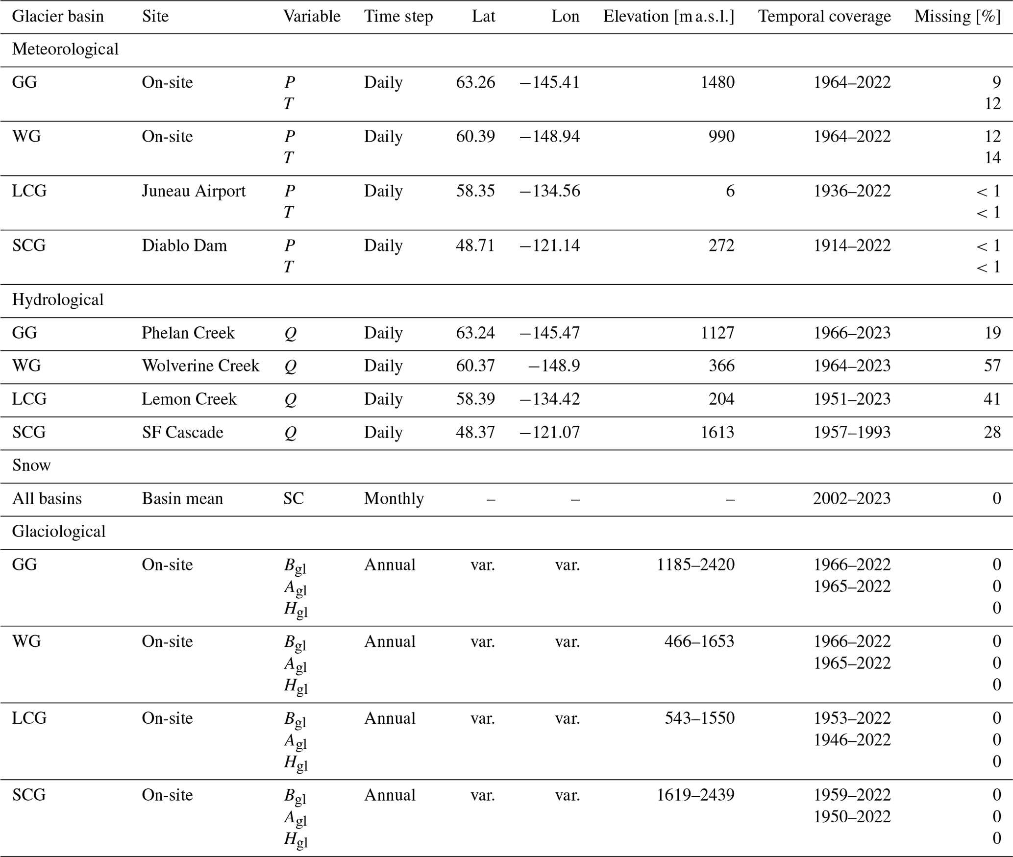
Continuous daily meteorological time series (precipitation and temperature) are directly available on-site for the GG and WG. However, although on-site measurements are also available for the LCG and SCG, the time series are rather short and show a relatively high number of missing values. For reasons of comparability, we follow the approach of O'Neel et al. (2019) and use the closest representative station, which is Juneau Airport (LCG) and Diablo Dam (SCG), respectively. The latter two are also part of the official data of the USGS Benchmark Glacier Project (Baker et al., 2018).
However, because SWAT-GL needs the minimum daily (Tmin) and maximum daily (Tmax) temperature, which were not continuously available in the project for the GG (starting 1995) and WG (starting 1997), a regression model was established to produce continuous daily Tmin and Tmax time series. In detail, daily mean temperature was used as a predictor of either Tmax or Tmin in the period where all three variables were available. Subsequently, the regression model was used to predict Tmax and Tmin backwards for the periods before 1995 (GG) and 1997 (WG). Data gaps of up to 3 days were linearly interpolated, and longer gaps were regressed using daily data from the closest meteorological station of each glacier. The approach is similar to O'Neel et al. (2019), with the only difference being that they used monthly regression for longer gaps. We also investigated the potential of the ERA5-Land (Muñoz Sabater, 2019) data to fill gaps, which was inadequate, especially due to a significant precipitation bias throughout the annual cycle and between years compared to the station data (see Fig. A1).
Hydrological data were obtained from the USGS National Water Information System (U.S. Geological Survey, 1994). We used the closest available gauge for each glacier to determine the total basin area. In detail, the discharge data of Phelan Creek (representing the GG basin), Wolverine Creek (WG basin), Lemon Creek (LCG basin) and the SF Cascade (SCG basin) were used. Details about the meteorological and hydrological sites and time series are found in Table 1.
Snow cover (SC) data were derived from the MOD10A1 and MYD10A1 V061 NDSI (Normalized Difference Snow Index) products with 500 m resolution. The NDSI is based on optical sensors from MODIS (Moderate Resolution Imaging Spectroradiometer) and is calculated as the difference between the reflection in the green spectrum (GREEN) and the short-wave infrared (SWIR) divided by the sum of the two (Dozier, 1989):
where INDSI is the NDSI and BGREEN and BSWIR are the green and SWIR bands, respectively.
For the classification of snow or no-snow pixels, an NDSI threshold of 0.4 was used, where values above 0.4 (Hofmeister et al., 2022) indicate snow pixels and smaller values are classified as snow-free. Daily fractional SC (%) on the basin and subbasin scale was then calculated as the average of snow-covered pixels within each basin. Subsequently, monthly aggregates were produced. MODIS NDSI data were available from 2002 up to now. A full overview of all datasets is given in Table 1. Auxiliary datasets used were elevation data from the Shuttle Radar Topography Mission (SRTM) (NASA JPL, 2013), the Randolph Glacier Inventory V6 (RGI) (RGI Consortium, 2017) and ice thickness estimates from Farinotti et al. (2019).
2.2 Study area
The locations of the USGS Benchmark Glaciers combined with the locations of the corresponding hydrological and meteorological stations used for each glacier are shown in Fig. 1. Note that the representative meteorological stations that were used to force the SWAT-GL models of the SCG and LCG are not shown, as they are situated outside of the basin boundaries (see O'Neel et al., 2019 for more details). In addition, the map contains the basin boundaries for each glacier, which were used as the model domain. The total glacier area in each catchment is slightly higher than the individual glacier area of each glacier, as the basins can include several adjacent glaciers. However, the main glacier fraction can be accounted to the four benchmark glaciers in each basin.
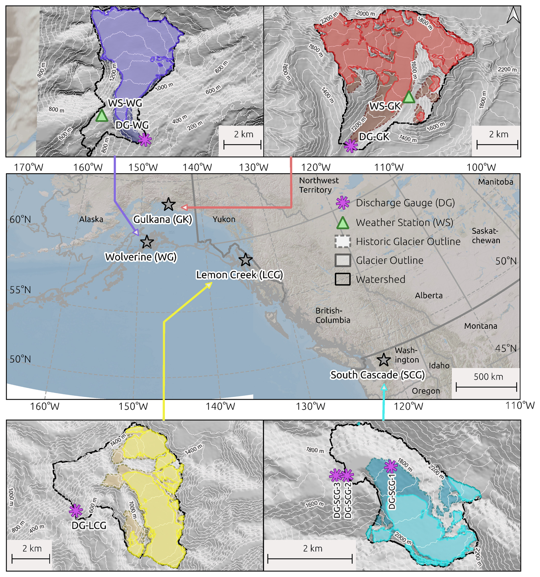
Figure 1Overview of the four USGS Benchmark Glaciers used in this study. Note that the SCG and LCG meteorological stations that were used are remote stations, which is why they are not visible in the map. The transparent outline refers to a historical date, and the filled outline, to a recent date. The dates are as follows: 1957/2021 GG, 1950/2020 WG, 1948/2021 LCG, 1958/2021 SCG.
The basins have an area of 28.4 km2 (GG, 64 % glaciated 2009), 23.9 km2 (WG, 69 % glaciated 2006), 29.3 km2 (LCG, 50 % glaciated 2005) and 5.9 km2 (SCG, 58 % glaciated 1958). Basin-wide glacier fractions were determined using Randolph Glacier Inventory data (RGI Consortium, 2017). Each glacier hereby represents a distinct climate regime, where the one located most northward (GG) is characterized by a continental (high-latitude) climate (O'Neel et al., 2014, 2019). WG, in contrast, is characterized by a maritime (high-latitude) climate regime (O'Neel et al., 2014, 2019). LCG represents another high-latitude maritime glacier, while SCG represents a mid-latitude maritime glacier (O'Neel et al., 2019; Horlings, 2016). All glaciers are retreating, with SCG showing the strongest relative recession, with a glacier area loss of more than 40 % (1.3 km2) since 1950. GG has lost around 18 % (3.3 km2) of its area since 1965, LCG decreased by 16 % (3.3 km2) from 1946 up to now and WG receded around 12 % (2 km2) compared to 1965. Glacier recession magnitudes reveal a gradient from north to south (O'Neel et al., 2019). Mass balance rates are provided in Fig. 3, which show an increasing negative (statistically significant) trend at all sites (O'Neel et al., 2019). According to O'Neel et al. (2019), total uncertainty, consisting of a geodetic and glaciological component, in the mass balance estimates is around 0.2 a−1, except for GG, where it is higher, with 0.4 a−1.
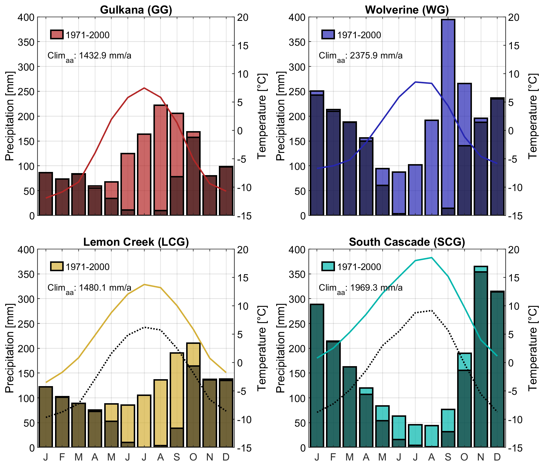
Figure 2Overview of the mean climate regimes of the four glaciers according to the stations of Table 1 and the reference period 1971–2000. Lines refer to monthly mean temperatures, and bars refer to mean monthly precipitation sums. As the LCG and SCG stations are remote and lower-elevated (20 and 40 km apart and at 6 and 270 m), black dotted lines representing temperature based on a −6.5 °C km−1 lapse rate are also provided. The letters from J to D correspond to the months January to December. Climaa refers to the annual average precipitation for the indicated periods. Black overlapping bars represent a solid precipitation proxy assuming that snowfall occurs when the temperature is below 1 °C.
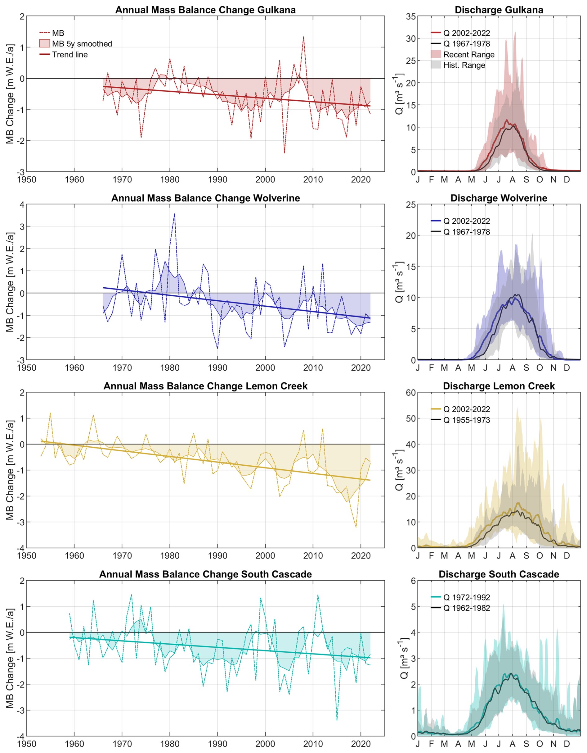
Figure 3Overview of the annual mass balance rates of all glaciers merged with the mean daily discharge of two periods for each glacier. The recent periods refer to 2002–2022 (GG, WG, LCG) and 1972–1992 (LCG), and the older periods refer to 1967–1978 (GG, WG), 1955–1973 (LCG) and 1962–1982 (SCG), as indicated in the day-of-the-year plots.
The following mean climate characteristics of each basin were evaluated based on the meteorological stations listed in Table 1 and the period 1971–2000. The continental GG, with an annual average precipitation of ∼1480 mm and a peak in August/September, is significantly drier than its maritime counterparts. SCG with an annual average of 1970 mm and WG with an annual mean of 2375 mm show the highest precipitation values among the four. While WG has its precipitation peak roughly in September/October, it also shows consistent high precipitation during the winter months and a dry period in summer. SCG is also characterized by a summer low, followed by an increase in precipitation during autumn and ending in a strong late autumn and winter peak (November–January). The annual precipitation totals of the LCG are around 1480 mm, with a less pronounced peak in autumn. The glacier generally has a lower gradient between wet and dry periods, which makes precipitation more evenly distributed throughout the year. In terms of temperature, all glaciers reach their maximum in either July or August and their yearly minimum in January. The mean climates are illustrated in Fig. 2. However, it should be noted that no lapse rates have been applied for the climate classification; the meteorological stations used for LCG and SCG come with an elevation difference of more than 500–1500 m (LCG) and 1300–2100 m (SCG). Lapse rates (temperature and precipitation) were later calibrated through the optimization procedure (see Sect. 3.3).
All gauges belong to intermittent streams, which can fall dry during the winter months (Fig. 3). While the corresponding streams of GG and WG had almost no flow in the available time series (see Table 1) from December to April/May, the streams of SCG and LCG carried water sporadically during these months. Annual average flows are 2.4 m3 s−1 (GG), 2.7 m3 s−1 (WG), 5.5 m3 s−1 (LCG) and 28.1 m3 s−1 (SCG), evaluated for the period 2002–2022 for all glaciers except SCG, where the years from 1972 to 1992 had to be chosen (due to a lack of observations). Inter-annual variability is highest at GG (coefficient of variation – CV – of 0.21) and lowest at SCG (CV of 0.13). Except for the SCG basin, we can see a tendency of a slight shift in the flow period towards an earlier onset of the melt season (Fig. 3).
2.3 SWAT-GL
The recently developed SWAT-GL (Schaffhauser et al., 2024) is a modified version of the traditional hydrological model SWAT (Arnold et al., 1998), which includes glacier dynamics based on the Δh approach developed by Huss et al. (2010). The empirical Δh-parameterization is called annually to translate the cumulative mass balance change to a change in glacier geometry. The concept assumes that lower elevated areas closer to the glacier terminus receive stronger ablation than higher elevated ones (Huss et al., 2008, 2010). Therefore, glaciers are divided into different elevation sections (ESs) for the application. In addition to its spatial distributed applicability, the method is mass-conserving and can be applied with glacier outlines and glacier thickness data only (Li et al., 2015; Seibert et al., 2018).
It basically consists of two modules: a mass balance and a glacier evolution module. Mass balance estimations are based on a degree-day approach, similar to the already existing snow routine of SWAT. Glacier evolution is implemented by means of the Δh approach (Huss et al., 2008, 2010). For detailed technical explanations, we refer to Schaffhauser et al. (2024), as we provide only a short summary of the main points here.
In general, the mass balance is formulated as:
where Wt represents the water equivalent of ice [mm H2O d−1] on day t, Mt represents the melt rate [mm H2O d−1], St represents the sublimation rate [mm H2O d−1], Ct refers to the accumulation rate [mm H2O d−1] and βf is an adjustable refreezing factor of ice during melt periods. Mt is calculated analogously to snow melt in the standard SWAT using a distinct melt factor.
The physical-based Δh-parameterization is able to simulate spatially distributed glacier retreat. The core of the approach is that glaciers are discretized into elevation sections, where each has an inherent storage and receives distinct ice thickness changes. The ESs are normalized for the glacier elevation range, and a characteristic (normalized) ice thickness change is assigned to each zone, according to:
where Enorm,i is the normalized elevation of ES i [–], Emax and Emin refer to the maximum and minimum glacier elevation [m], respectively, and Ei is the actual elevation of ES i [m].
Lower altitudes hereby receive stronger ablation than higher ones. The characteristic ice thickness change for each normalized elevation varies with glacier size. One of three parameterizations is used separately for each glacier, which are thus classified as small (<5 km2), medium (5–20 km2) or large (>20 km2). The empirical relationship is illustrated in Fig. 4. It is important to note that the Δh-parameterization is called annually (at the end of a glaciological year) to redistribute (lumped) annual mass balance changes over the individual ESs of a subbasin to simulate glacier retreat. The normalized ice thickness change formulas of Fig. 4 follow the general form:
where a, b, c, y are coefficients that vary with glacier size and Δhi represents the normalized ice thickness change for an elevation Ei. We use the parameters based on Huss et al. (2010). Theoretically, the parameters could be derived specifically for any glacier if the required data are available (e.g., two digital elevation models (DEMs) on different dates). The dimensionless ice thickness change Δhi is rescaled using a scaling factor fs [m] to receive the change in meters for every glaciological year (5):
with Va referring to the annual glacier volume change, expressed in water equivalent [m3], that is calculated by multiplication of the annual EW values (see Eq. 2) with the subbasin area. Ai is the area of ES i, with n being the total number of ESs. Annual ice thickness changes are then calculated via:
where hi,1 is the updated ice thickness [m water equivalent] after each glaciological year of ES i and hi,0 is the ice thickness [m water equivalent] in ES i before the application of Δh parameterization. If hi,1 is ≤0, the ES is assumed to be ice-free, causing an update of the glacier extent.
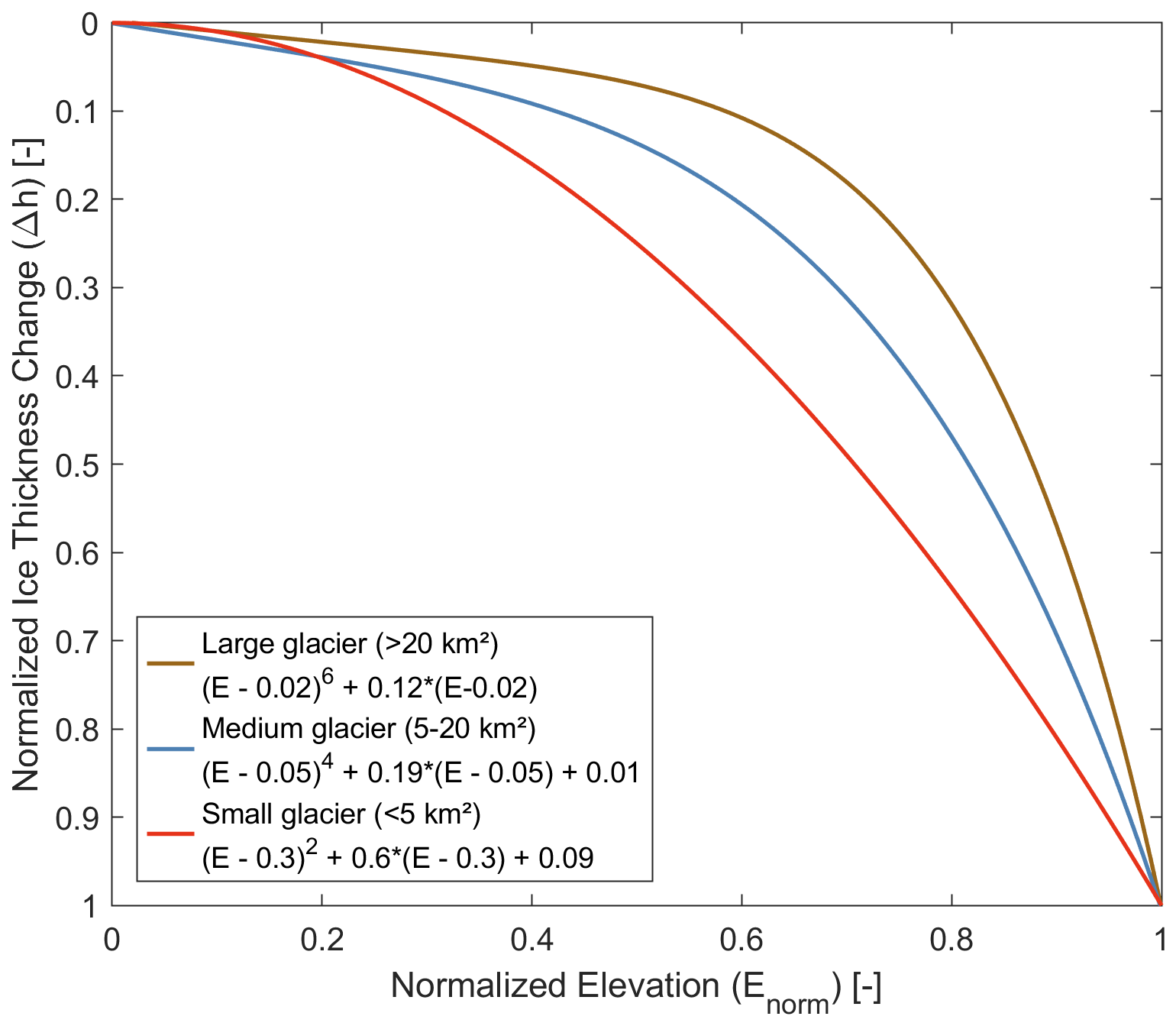
Figure 4Empirical relationship between normalized glacier elevation and the normalized ice thickness change based on Huss et al. (2010).
SWAT-GL classifies glaciers on the subbasin scale, meaning that a simplified assumption is used where all glaciated areas within a subbasin are considered as one glacier object. The implementation of the glacier routine in SWAT introduces five new parameters that control glacier melt (and refreezing) and accumulation. In addition, one new output file containing annual glacier mass balance information (for each glaciological year) and two new input files that require some preprocessing are introduced. The two input files refer to the parameterization on the HRU scale and the glacier initialization with respect to hypsometry, ice thickness and volume. The source code of SWAT-GL, together with an example, is freely accessible from GitLab (https://gitlab.com/lshm1/swat-g, last access: 21 July 2025).
2.4 Sensitivity analysis
In order to provide a comprehensive picture of SWAT-GL, we also performed a global sensitivity analysis using the Morris method (or elementary effects) (Morris, 1991; Saltelli et al., 2008). The method, which is based on a multiple-starts perturbation approach and thus belongs to the one-at-a-time (OAT) methods, is able to determine approximate sensitivities at a relatively low computational cost (Saltelli et al., 2008; Pianosi et al., 2016). A lower computational cost hereby refers to the fact that the total number of simulations required is significantly reduced compared to other methods, such as for the Sobol method. The EEs test has thus been established as a robust method for screening and ranking of the input factors (Pianosi et al., 2016).
For sampling, we used the radial design, where r sample points from a Latin hypercube sampling serve as well-spread starting points in the input space (Campolongo et al., 2011). The total sample size N follows the form r(M+1), with M being the number of input factors. For r, a value of 500 was chosen, resulting in 7500 model evaluations (M=14) (Sarrazin et al., 2016). A value of r=500 can be considered as sufficient for screening and ranking purposes; for example, Vanuytrecht et al. (2014) has shown that a stable ranking can be achieved using only 25 trajectories, whereby the relatively small numbers of simulations necessary for ranking were further confirmed by Nossent et al. (2011). The basic idea of the radial design is that, from a starting point, one factor M is varied while keeping all others fixed. This results in M steps (varying each factor once) that are performed for each sampling point (r). In general, r EEs are calculated per input factor, which are then averaged to provide a global sensitivity metric μi for each input factor i. The calculation itself is based on finite differences. To account for non-monotonic effects in the model, is used based on the absolute values of the EEs (Campolongo et al., 2011). The formulation is:
An EE of an input factor i can be calculated as follows:
with IEE,i being an elementary effect of input factor i, being the individual values of the factors and Δ being the step (or perturbation). We also calculated the standard deviation σi of the EEs as a proxy of the interaction of input factor i with the other factors. It also describes whether the model output is linearly or non-linearly affected by an input factor (Garcia Sanchez et al., 2014; Merchán-Rivera et al., 2022). To avoid confusion with other sigmas used in this work, we define the sigma of an EE as σEE,i. The ratio of also provides insights into whether the effect of a factor is monotonous or almost monotonous, as explained in Garcia Sanchez et al. (2014) and Merchán-Rivera et al. (2022). This is especially important to derive information on whether the interaction of snow and glacier processes is represented (adequately). Due to the different scales of the input factors, the standardization of Sin and Gernaey (2009) was applied. The SA is used to support and complement the benchmarking procedure to (i) determine the importance of the newly introduced parameters under different conditions, (ii) rank the parameters to get insights into how the most influential parameters differ between the catchments and (iii) identify whether the glacier routine interacts appropriately with the snow routine. For the SA, the combined calibration period from 2002–2015 and validation period from 2016–2022 was used.
2.5 SWAT-GL testing methodology
The core of the study is to evaluate the capabilities of SWAT-GL to simulate multiple glaciological components in glaciated catchments. This involves the assessment of SWAT-GL based on the representation of multiple snow and glacier variables in the four glaciated catchments. The glacier- and snow-optimized SWAT-GL model is further compared with a discharge-only and mass-balance-only optimized SWAT-GL model. Lastly, two SWAT standard models are introduced that do not consider glacier processes and serve as upper and lower benchmark estimates in comparison to SWAT-GL.
2.5.1 Preprocessing and initialization
SWAT-GL needs distributed glacier thickness and glacier area information as input for each ES and subbasin. However, these data are usually not easily available for various years. In most cases, only globally and openly available datasets such as glacier areas from the RGI (RGI Consortium, 2017) and ice thickness from Farinotti et al. (2019) or Millan et al. (2022), representing a fixed point in time, are available to use. Alternatively, if geodetic information is available at different times, glacier thickness can also be directly inferred for each of them. As the USGS Benchmark Glacier Project provides geodetic data for several years, we have chosen the best available DEM closest to the mass balance observation start of each glacier. “Best” hereby refers to full coverage of the glacier basins along with a minimum of missing values. The thickness was then estimated using the GlabTob2 model (Linsbauer et al., 2009, 2012; Frey et al., 2014). Glacier outlines were also available at several times in the benchmark project, and the year closest to the chosen DEM was selected to initialize SWAT-GL. If a mismatch between DEM and glacier outline acquisition year and mass balance observation start was present, we corrected the initial glacier volume by adding the mass loss or gain that happened since the observation started to the DEM acquisition year. For example, if mass balance measurements started in 1966 and the best DEM and glacier outline was available from 1977, the cumulative mass balance estimates until 1977 were added to the initial volume. The volume was then distributed to the individual ESs while maintaining the original volume fractions of the bands in the total volume. ES sections were defined with a spacing of 100 m.
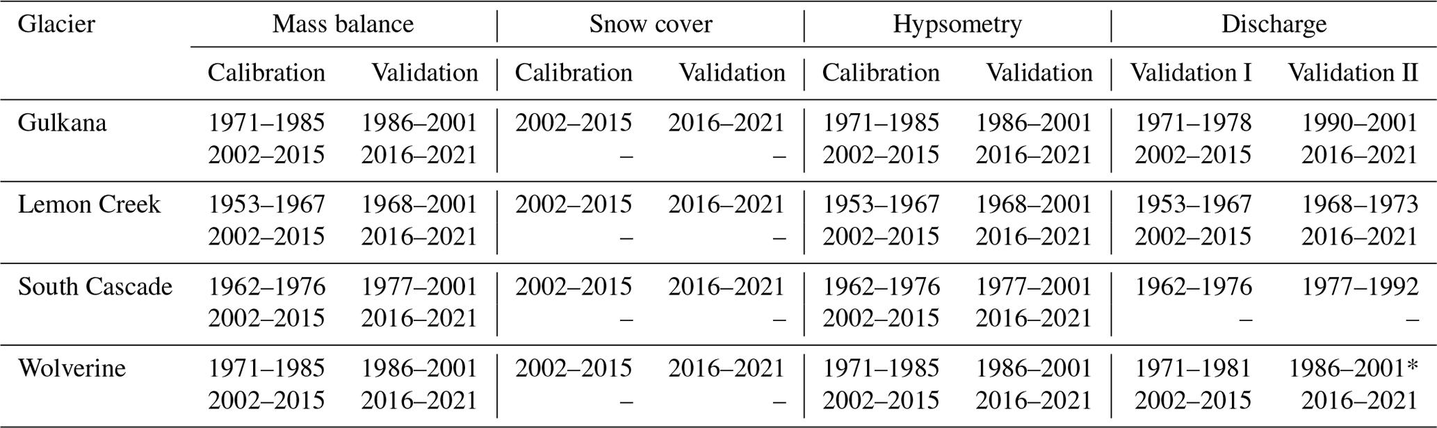
A model run comprised the full available glaciological time series of each catchment, due to differences in the availability of snow cover and the glaciological components. Thus, across glaciers, calibration phases can differ. For example, the glaciers were initialized for the starting year of the mass balance time series (GG 1966, WG 1966, LCG 1953, SCG 1959), while MODIS SC was available from 2002 onward. SC was therefore calibrated from 2002 to 2015 and validated for the period 2016–2021. For glacier mass balances and glacier hypsometries, two calibration phases were used (in contrast to snow cover), one which was the same period as for snow cover (2002–2015) and one at the beginning of the model run (GG 1971–1985, WG 1971–1985, SCG 1962–1976, LCG 1953–1967). Discrepancies in the first calibration and validation phase across glaciers stem from different measurement starting dates. The aim was to make use of the full glaciological time series to account for transient behavior in the models. The remainder of the time series was then used as the validation phase (one period matching the one of snow cover (2016–2021) and one covering the remaining time series at the end of each glacier's first calibration phase up to 2001). The second validation phase was used in order to make full use of the available information and to assess SWAT-GL over a long timescale. The summary of the temporal settings is given in Table 2. Note that the periods for discharge were intended to match those of the other variables; however, data restrictions did not allow a perfect match.
Table 2Overview of the calibration and validation phases. Note: as discharge was used for cross-validation purposes only, it thus has two validation phases rather than a calibration and validation phase. For the SCG, no discharge data were available for the 2000s, leading to only one validation period. The asterisk for the WG indicates that validation period II is rather poor due to mainly missing values. For snow cover only, one calibration and validation phase was used due to the relatively short temporal coverage of the product, while for glacier variables, two calibration and validation periods were used. A minus sign indicates that a specific second calibration or validation period was not used for this variable.
2.5.2 Multi-objective optimization
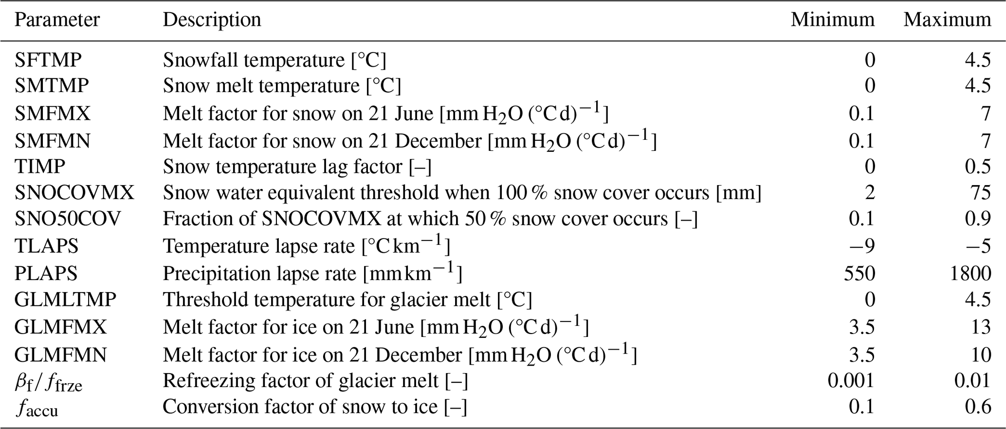
Although hydrological models traditionally focus on discharge simulation, which is also one of the main goals of SWAT-GL, the glacier routine will be assessed primarily with respect to representing glacier and snow processes. Given the relevance of discharge, the variable will be presented alongside for cross-validation purposes. It is assumed that an adequate discharge representation in heavily glacier- and snow-dominated catchments could be achieved by a reasonable representation of the snow and glacier components. In detail, we calibrated and validated each of the four models based on snow cover (monthly), glacier mass balance variations (annual) and glacier hypsometries (annual) using an automated multi-objective optimization (MOO). As mentioned, discharge simulations (from daily to annual) are also provided to evaluate the model consistency of SWAT-GL. Given the snow- and glacier-focused optimization, only parameters related to SWAT's original snow routine and the newly introduced glacier routine in SWAT-GL were used for the MOO (see Table 3). As a result, 14 parameters were considered in the MOO. We used an automatic MOO procedure, where each of the three prescribed variables referred to one objective (SC, MB, hypsometry). The optimization was performed using the widely used evolutionary NSGA-II (Nondominated Sorting Genetic Algorithm) algorithm (Deb et al., 2002). Based on nondomination sorting and the introduction of a crowding distance operator to favor solutions that are less-crowded (high crowding distance), NSGA-II iteratively finds solutions that are uniformly spread at the Pareto front. The population size of a generation was 100, and the maximum number of generations was set to 100. We used simulated binary crossover with a crossover probability of 0.9 and polynomial mutation with a mutation probability of 0.3.
Table 3Parameters and their relative ranges used for the benchmarking of SWAT-GL.
For glacier and snow variables, a normalized root-mean-square error (fNRMSE), based on the standard deviation of the observations of each variable, was consistently used as the objective function (OF) (Eq. 10). The fNRMSE increases comparability between the individual OFs and allows minimizing the residuals between observed and simulated values of all variables. For snow cover, we excluded winter months in the optimization procedure to put more weight on the months where snow cover is dynamic, as snow cover is usually 100 % from December to at least April. The effect is more pronounced in basins with less snow cover dynamics and therefore a relatively high minimum summer snow cover. The simulation of a permanent snow cover then leads to good OF values. We will further discuss this issue later in the paper. The standard form of fRMSE can be defined as follows:
with Ox,t being observed and Sx,t being simulated components of variable x, which is either snow cover, glacier mass balance or hypsometry, t refers to the time step (monthly or annual depending on the variable), and n represents the number of available data points. The standardization follows the form:
where σx is the standard deviation of the observations of each variable.
However, as glacier hypsometries provide areal time series for multiple glacier elevations, the individual fRMSE of each elevation was calculated and then averaged to obtain one fRMSE value, which was standardized in a last step using the standard deviation of the observed total glacier area. This gives a more equal weight to all elevations to get rid of solutions where individual elevations might have a high non-standardized error. In other words, if using an average of the fNRMSE of all individual elevations, those with small observed standard deviations (e.g., higher-elevated and less dynamic ones) could lead to an excessive degradation of the overall OF. fPBIAS is used to show the difference between simulated and observed cumulative mass balance at the end of the simulation period and can be formulated as:
with the same declarations as above.
Discharge, used for cross-validation purposes, is based on the Kling–Gupta efficiency (KGE), which is calculated as:
where r refers to the Pearson Correlation, α to the error in flow variability and β to the bias term, with:
where σ and μ refer to the standard deviation and mean of the simulation and observation, respectively.
2.5.3 Statistical tests
The results for all variables focus on the last generation of the optimization and the best simulations of each variable. Apart from the described methodology, we tested SWAT-GL's ability to reproduce observed mass balance nonstationarities, inter-annual variability, and the monotonic relationship between simulated and observed mass balance. For this purpose, the full time series was used, homogeneity was tested with the Wilcoxon rank-sum test (WRS) (Wilcoxon, 1945) and the Pettitt test (Pettitt, 1979), and trends were detected using a modified Mann–Kendall (MK) version from Hamed and Ramachandra Rao (1998), which considers autocorrelation. For the WRS, the first calibration and the last available validation periods were used. Statistical tests are applied to give an indication whether SWAT-GL is generally able to deal with potential nonstationarities in the catchments, as the model is applied for relatively long simulation periods.
2.5.4 Single-objective optimization of SWAT-GL and benchmarking with the SWAT standard
Lastly, for demonstration purposes, a single-objective optimization (SOO) was conducted using differential evolution (DE) (Storn and Price, 1997) and the adaptations described in Dawar and Ludwig (2014). The SOO demonstration was performed as an example for the WG and two variables, namely, mass balance and discharge. For discharge, an additional standard SWAT model without the SWAT-GL glacier extensions was set up for benchmarking purposes, taking the benchmarking approach by Seibert et al. (2018) and slightly modified by Merk et al. (2024) as orientation. The standard SWAT model, not considering glaciers adequately, provided a lower benchmark (LB) for the discharge representation, using the median value of 1000 random Latin hypercube samples. As the upper benchmark (UB) for discharge, again, a SOO analogous to the one from SWAT-GL was performed. In summary, the comparison consisted of five models for discharge (three SWAT-GL, two SWAT standard) and three for mass balance (all SWAT-GL due to the missing components in the SWAT standard). An overview is provided in Table 4.
Table 4Overview of models used for the comparison and evaluation of SWAT-GL.
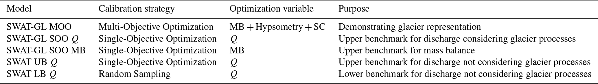
The results of the mass balance SOO model were compared with the results of the MOO introduced previously (covering MB, SC and hypsometry), while the results of the discharge SOO model were also compared with the LB and UB SWAT models for discharge. The results exemplify how MOO models in glaciated catchments compare to SOO benchmark models for pure discharge or mass balance calibrations, which is common in hydrological studies. The results therefore demonstrate the impacts of SOO models on general model consistency, missing trade-offs, and the structural differences between SWAT and SWAT-GL. Discharge was evaluated based on fKGE, and mass balance again on fNRMSE. The time periods are equal to those in Table 2. For the SOO of discharge, the following additional parameters were included: to account for lags in discharge as well as the general infiltration behavior, SURLAG (surface runoff lag) and CN2 (curve number for moisture conditions II) parameters were introduced for the SOO of discharge in contrast to the MOO parameter space of Table 3. The LB and UB models that use the SWAT standard share the same parameters and ranges as the discharge SOO model, except for the five glacier parameters available only in SWAT-GL and not in the standard SWAT.
In the following, the results of the Morris SA and SWAT-GL MOO are presented, complemented by results providing details on the final parameterizations derived from the MOO and results indicating SWAT-GL's representation of inhomogeneities and variability as well as SWAT-GL's representation of discharge. First, the results of the SA are shown (Sect. 3.1), followed by an overview of the final parameter sets across all catchments (Sect. 3.2). Afterwards, the results of SWAT-GL's MOO are illustrated, which represent the main purpose of the paper (Sect. 3.3). The MOO results are supplemented by a short statistical analysis focusing on whether SWAT-GL captures inhomogeneity and variability appropriately (Sect. 3.4), as well as results on how the MOO (excluding discharge) is capable of simulating discharge (Sect. 3.5). Lastly, the results of the two SOO SWAT-GL models that were optimized using discharge and mass balance and the two SWAT standard models serving as LB and UB estimates of discharge are compared to the MOO results of simulating the mass balance, discharge and snow cover (Sect. 3.6).
It is important to note that discharge was excluded from the MOO procedure, as the primary objective of the study is to evaluate SWAT-GL's ability to represent snow and glacier processes. However, given that all catchments are strongly driven by snow and glacier processes, discharge simulations from the MOO are discussed and further compared to a SOO model that solely considers discharge and, therefore, can be seen as an upper benchmark for the discharge representation in these catchments by SWAT-GL.
3.1 SWAT-GL's glacier and snow parameter sensitivity
The SA is based on the EEs method. Our results for all catchments are presented as a scatterplot between μ*, the mean sensitivity of a factor (parameter) and σ as proxy for the interactions of a factor (Fig. 5).
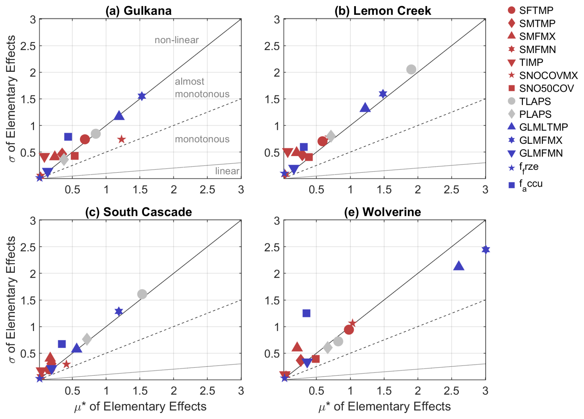
Figure 5SA results based on the EEs method for all four catchments and 14 parameters. The slopes () of the different lines, which classify parameter effects on the model outputs as linear, monotonous, almost monotonous and non-linear, are as follows: 0.1 (dotted line), 0.5 (dashed line), 1 (solid line). Red signs refer to snow parameters, gray indicate lapse rates and blue indicate glacier parameters.
A common pattern that all catchments share, albeit to varying extents, is their spread around the 1:1 line that differentiates between non-linear and almost-monotonous effects (Garcia Sanchez et al., 2014). Moreover, it is shown that, in general, the more sensitive parameters (larger μ*) tend to have higher interactions and stronger potential non-linear model responses. It is also shown that the model response of all catchments strongly depends on GLMFMX (blue hexagon), which controls the maximum value of the degree-day factor of ice (and thus the amount of glacier melt that can occur at a specific day of the year). In terms of factor ranking, GLMFMX is the most or the second-most influential factor. It is the most important parameter in the WG and GG basins, where the respective meteorological stations are located directly at the glacier. However, GLMFMX is substituted by the temperature lapse rate (TLAPS, gray circle) at the SCG and LCG, where the respective meteorological stations are located outside the catchment and at a significantly lower elevation than the glaciers. Due to the difference in altitude (which is part of the precipitation correction formulation) between station and elevation band centers, it is inherent that the lapse rates become more important. Due to the temperature dominance of both snow and glacier processes, the sensitivity of the precipitation lapse rate (PLAPS, gray diamond) is less pronounced and strongest at the high-elevated SCG. Among the four most important factors is the threshold temperature of glacier melt (GLMLTMP, blue upward triangle), which controls the onset of melt and has an effect on the timing of melt events and the amount of melt. The temperature lapse rate and glacier melt temperature can favor similar conditions or act contradictory (a decrease in melt temperature favors earlier melt onset and small or no temperature lapse rate). In general, SWAT-GL is strongly temperature-dominated in all catchments.
However, the relevance of precipitation in the SCG basin might be a special characteristic (with regard to the PLAPS ranking in the other basins). In addition, except for the SCG and LCG, SNOCOVMX (red pentagon) is ranked among the four most sensitive parameters. The parameter determines a threshold of snow water equivalent (SWE) that corresponds to a 100 % coverage of snow. As glacier melt can occur only when the glacier is snow-free, the parameter directly affects glacier melt, which explains its relevance in the catchments.
Overall, the ranking shows that, across all basins, GLMFMX, TLAPS, GLMLTMP, SNOCOVMX and PLAPS are found to be most often among the most influential parameters.
With respect to potential interactions and non-linear model responses, the accumulation factor (f_accu, blue square) that is responsible for the snow metamorphism (or turnover from snow to ice) takes a dominant role at the WG, GG and SCG. This is plausible, as it couples snow and glacier processes by transforming a specific fraction of snow lying on the glacier to ice and thus affects both storages. Although it is not among the most sensitive factors, it can have a high significance in certain situations due to its possible interactions. Although the most influential parameters receive high σEE values, they do not necessarily fall in the non-linear area (GG, WG). The strong non-linearity visible for the SCG and LCG might be caused by the fact that the underlying measurement stations are located outside the catchments at relatively low elevations. All models generally show a non-linear or monotonous behavior and are potentially characterized by interactions rather than a linear relationship.
Additionally, we identify around six to eight parameters that are less or non-influential, which would reduce the dimensionality of the parameter space for the respective models. However, given the strong interactions of the parameters, the parameter space was kept constant, including the entire space.
3.2 Inter-basin comparison of optimized glacier parameters
A comparison between the values of the final parameter sets of all catchments is shown in Fig. 6. As the main purpose is to evaluate the glacier routine introduced in SWAT-GL, the comparison is limited to the five glacier parameters. Results are presented for the fNRMSE values of the annual glacier mass balance only. The parameter values of the GG are relatively well-spaced in the parameter space, with the exception of the GLMFMX parameter, which controls the maximum amount of glacier melt. The parameter tends to cluster at its lower boundary for GG, LCG and SCG. The lower bound of GLMFMX is associated with a reduction in strong negative mass balance rates, which might lead to an overestimated ablation. The parameter is among the most interactive ones, as shown before, indicating that parameter clustering does not necessarily result in a distinct objective function distribution. As Fig. 6 provides only a snapshot for the fNRMSE of MB, the pattern of the objective function space for SC, for example, could look different. Analogous to GG, the final parameterizations of the LCG are generally well-spread. An exception is the glacier melt temperature (GLMLTMP) and GLMFMX, which both show clustered values. In contrast to the maximum melt factor, the glacier melt threshold temperature groups at its (relatively high) upper bound for the LCG, WG and SCG. The two patterns indicate the necessity of high melt rates, which should not occur too early. The final parameter distribution of the WG is more narrow compared to the other catchments. It is shown that, especially for the accumulation rate (faccu), small values are desired to avoid large positive mass balance simulations.
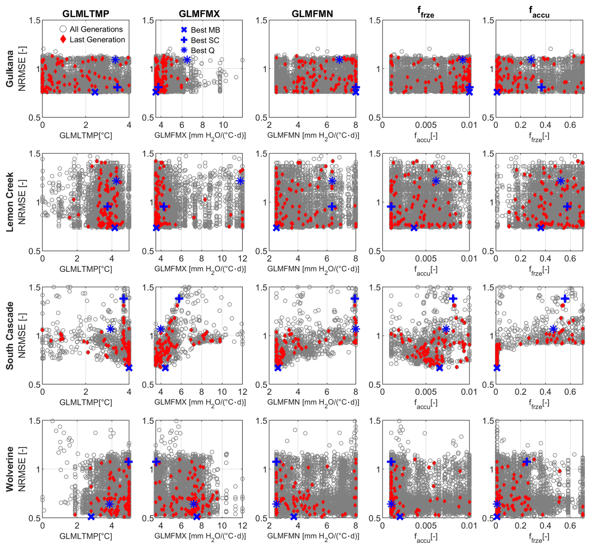
Figure 6Parameter space illustrated for all glacier-related parameters for all generations (gray) and the final generation (red). The shown fNRMSE values refer to the results of annual glacier mass balance simulations. The three blue symbols refer to the individual best solutions for the mass balance, snow cover and (cross-validated) discharge in the last generation. “Best” hereby means either the lowest fNRMSE (for SC or MB) or the highest KGE (for discharge) within the last generation.
Looking at the best parameters for different objectives, it is shown that the best SC simulations can deviate significantly from the best MB simulations (in both the difference in fNRMSE of the MB and the parameter values). Large deviations in terms of the fNRMSE of the MB can be seen for the SCG and WG (large vertical difference of blue cross and x). With respect to the best final parameters of these two variables, large differences can be observed for GLMLTMP, GLMFMX of the WG (large horizontal distance of blue cross and x), and GLMFMN of the SCG and LCG. Moreover, it already becomes apparent that the best discharge simulations do not necessarily coincide with the best simulations of the glacier mass balance or snow cover, despite the strong dependency of discharge on snow and glacier melt, which is further discussed in the following sections.
Table A1 provides a detailed overview of the ranges and median values for each glacier parameter and each catchment at the end of the optimization.
3.3 Evaluating SWAT-GL's representation of glacier and snow processes
The performance of the optimization procedure is shown in Table 5. Statistical results for discharge are presented alongside the other variables for demonstration purposes, although it was not part of the optimization procedure. The results for discharge comprise two validation periods, which were chosen analogously to the ones for the glacier mass balance, if data were available.
Table 5Performance of SWAT-GL for all variables and glaciers with respect to the best simulation of the last generation of the optimization procedure. Numbers in brackets belong to the initial results based on a Latin hypercube sampling and serve as starting values for the optimization to provide an indication of the optimization performance. Note: discharge was not calibrated but is only shown for cross-validation purposes. Discharge thus has two validation phases, following the periods assigned to the glacier mass balance evaluation of each glacier (see Sect. 3.3). “Cum. Bgl” refers to the mismatch between observed and simulated cumulative mass balance at the end of the time series and is therefore not attributed to any of the calibration or validation periods. Negative values of Cum. Bgl indicate that the model is underestimating mass balance losses. Optimal values for fNRMSE and fPBIAS are 0 and 1 for fKGE, respectively.
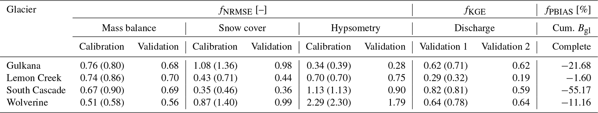
With respect to glacier mass balance estimates, the lowest fNRMSE values were found for the WG model (both calibration and validation), followed by the SCG model. In contrast, the WG model shows the worst performance w.r.t. hypsometries, for which the best performance was reached in the GG basin. Concerning snow cover, the LCG and SCG models achieve the best performance metrics in both the calibration and validation periods (0.43 and 0.44 for the LCG model; 0.35 and 0.36 for the SCG model). Slight variations were observed between the calibration and validation phases for any of the objective functions of all variables included in the optimization procedure. It should be noted that a direct inter-comparison of the absolute fNRMSE values between the catchments is difficult, as the standard deviation of the observations used for the normalization has a dominant effect on the values. For example, the standard deviation of the mass balance observations of the WG is a factor of 1.6–9.4 higher than that of the other glaciers (calibration period). The same applies for the snow cover results of the SCG, where observed snow cover standard deviations are 1.3–2.4 times higher than those of the other glaciers.
A clearer picture emerges from the graphical representation of the optimization results in Fig. 7. The discrepancy at the end of the simulation periods of the cumulative mass balance ranges from −1.6 % to −55.17 %. The relatively large outlier of −55.17 % arises from the SCG, where the mass balance loss stagnates in the 1990s. The abrupt change in the mass balance is also indirectly reflected in the cross-validated results of discharge. While fKGE in the beginning of the simulation is around 0.82, a significant drop to 0.59 can be observed in the second evaluation period. Problems in the SCG model become especially apparent when focusing on the lower bound of the model range (gray shading in Fig. 7 of the cumulative mass balance). Here, we notice a very poor representation of the inter-annual signal, as the simulations show two very abrupt drops and long periods of stagnation. It is likely that the glacier has retreated to altitudes that are not subject to temperature-induced melting. The wide range visible in the cumulative mass balance could be caused by only a few solutions and does not allow for conclusions about the real distribution of the final simulations. We thus show in Fig. A2 the individual cumulative mass balance representations of all optimized solutions together with the distribution of the cumulative mass balance at the end of the simulation period (all 100 values of the last year of simulation for each glacier). It is found that the upper bound of the GG and WG and the lower bound of the LCG and SCG are caused by a small subset of solutions. The LCG, with an almost perfect fit at the end of the simulation period, is nevertheless overestimating ablation for a large part of the simulation period. Overall, the models are underestimating ablation rates after the 2000's (with the exception of the WG). This underestimation becomes even more evident by looking at the annual mass balance rates (last column of Fig. 7). All models perform well in simulating monthly snow cover in both the calibration and validation phase. The spread of the models (gray shading) is relatively large and includes simulations with almost no snow cover in summer. The WG has a period of positive mass balance in the 1980s, which is likely causing the upward tendency of the simulation range (the share of simulations with a positive cumulative mass balance until the end of the simulation).
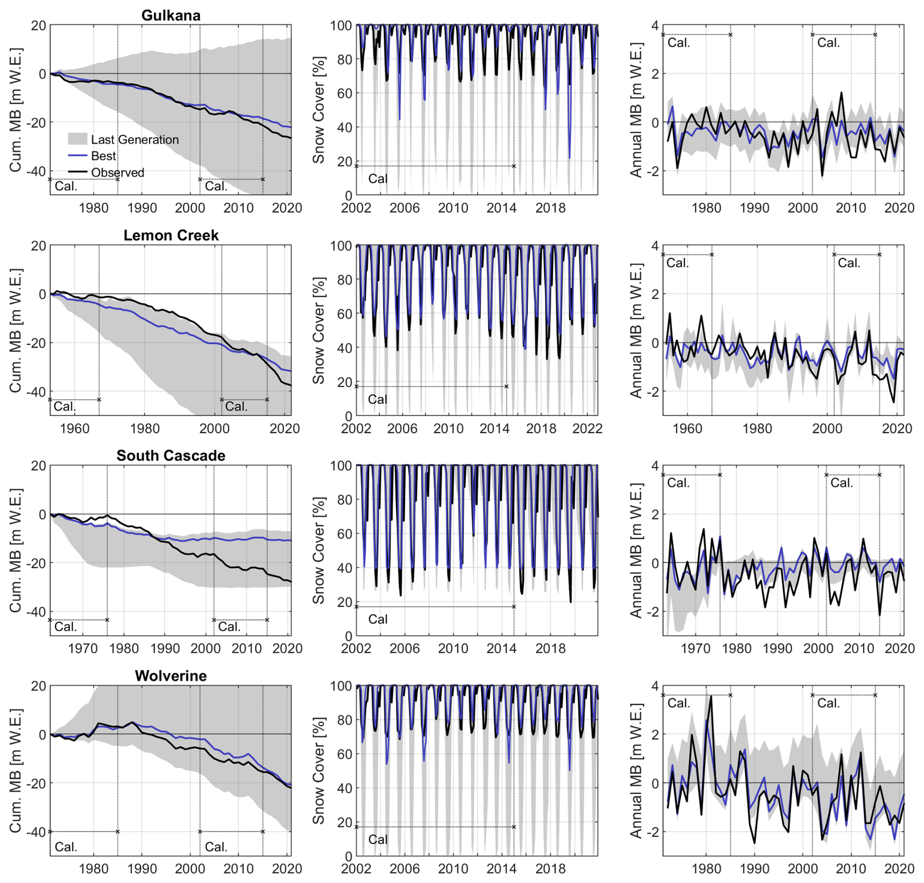
Figure 7Simulation results of the last generation of the optimization procedure for the cumulative mass balance (Column 1), monthly snow cover (Column 2) and annual mass balance (Column 3). Each row corresponds to one glacier. Blue represents the best evaluation of the last generation for the respective variable, black refers to observations and gray shadings indicate the range of all evaluations of the last generation. The dashed lines with the “Cal.” annotation indicate the individual calibration phases of each study area. The remainder of each time series was used for validation.
In summary, the objective function values indicate that SWAT-GL is generally capable of representing the glacier dynamics, with the exception of the SCG, which shows a sharply declining drop in performance over the course of the simulation period. However, a benchmark model would be necessary for an absolute interpretation of the values.
3.4 SWAT-GL's ability to capture mass balance inhomogeneity and variability
As SWAT-GL was tested for relatively long simulation periods, its capabilities to capture potential inhomogeneities present in the mass balance observations are evaluated. Furthermore, it was investigated how mass balance variability, e.g., represented by the coefficient of variation (CV) as a proxy for inter-annual variability, is represented by SWAT-GL. Inhomogeneities were determined by a trend detection based on a modified Mann–Kendall and additionally using the Pettitt and Wilcoxon rank-sum (WRS) tests. The null hypothesis of both methods is that the time series contain no change. All results are provided in Table 6. The results of the MK, WRS and Pettitt tests are provided as integers, 0 or 1, indicating whether the null hypothesis was rejected (1) or not (0).
Table 6Summary of statistical results for the simulated and observed mass balance time series over the whole simulation period. The summary table consists of the Spearman correlation (ρ), the modified Mann–Kendall after Hamed and Ramachandra Rao (1998) considering autocorrelation (MMKH), the Sen's slope estimator, the coefficient of variation (CV), and the Pettitt and Wilcoxon–Rank Sum (WRS) tests. Results of the MK, WRS and Pettitt tests are provided as integers, where 1 indicates that the null hypothesis was rejected and 0 indicates that it was accepted.
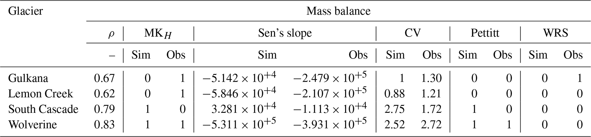
While the Spearman correlation suggests a satisfying to good agreement in the monotonic relationship between simulated and observed mass balance in all catchments, the models failed to represent the trend detection results of the observations. Based on the modified Mann–Kendall test, which takes serial correlation into account, SWAT-GL was able to correctly classify the trend statistic in only one catchment. The Sen's slope estimator, used to represent trend magnitudes, differed, especially for the outlier SCG model, where the sign was mismatched. In the WG and LCG models, the simulated trend component was underestimated, while it was overestimated for the WG. The CV, with generally large values mostly above 1, was underestimated in two cases and overestimated in two cases. While it was general in an acceptable range, the SCG again exhibited an outlier. The annual mass balance time series, which were trend-corrected in the presence of a trend, were further tested on inhomogeneities based on the non-parametric Pettitt and Wilcoxon rank-sum tests.
In summary, the simulations agreed relatively well with the observations at the 0.05 significance level. However, SWAT-GL did not capture the shift in the median detected in the observed time series of the GG (based on the WRS) and additionally rejected the null hypothesis of the Pettitt test for the SCG. However, it can be observed that poor SCG simulations affect the significance of test results.
3.5 Cross-validation of discharge
Discharge in all catchments was cross-validated on the daily scale, assuming that a reasonable fit is achievable, when glacier- and snow-related processes are well represented in the heavily glaciated catchments. The performance, evaluated based on fKGE, can be found in Table 5. The temporal coverage of the validation periods of each catchment is found in Table 2.
First, we see that the GG and WG models show no difference in the fKGE values of the respective validation periods. Second, a significant drop in quality for the SCG model (from validation phases 1–2) is found. Lastly, the LCG model acts as a strong outlier, with fKGE values In contrast, the other three catchments almost entirely show fKGE values >0.6, results often considered satisfactory in hydrological studies according to the classifications of Moriasi et al. (2007) and Moriasi et al. (2015). Interestingly, the worst-performing glacier during the glacier-based optimization (SCG) exhibits the best overall discharge performance. Its good quality in the first validation period stems mainly from an overestimated ablation that reduces the underestimation of available water for discharge compared to the other glaciers. Given the large glacier influence in the catchment, the good performance w.r.t. discharge is likely caused for wrong reasons. This result stresses the fact that models that are evaluated only for discharge are questionable for comprehensive hydrological investigations. The other glaciers are characterized by a high fPBIAS towards the observations (simulations have less water than observations). The second validation phase of the SCG model, in contrast to the other glaciers, does not cover the 2000s, which are associated with even higher instationarities. Covering the 2000s would likely further reduce the performance metric. fPBIAS is larger in the LCG model, where streamflow is underestimated by 45 % and 51 % in the calibration and validation phases, respectively.
In addition to the daily performance of Table 5, we further evaluate mean annual flows, as illustrated in Fig. 8, together with two separate periods of simulated mean daily discharge (average discharge for each day of the year over the indicated periods). For the WG, LCG and GG models, a distinct underestimation of annual flows is present in the simulations. When annual flows are centered (mean corrected), a good monotonic relationship for the WG model is observed (see Fig. A3). For the SCG, the deviation of observed and simulated annual discharge increases over time. This further indicates that a temporal coverage of the 2000s of the SCG model would further degrade its results. The annual dynamics of the LCG and GG are only partially met, and the larger positive anomalies of the LCG are not captured by the model. The results suggest that inter-annual discharge variability is slightly lower in the model than that observed. In general, simulated annual flows of the SCG show a decreasing tendency with time, which could be caused by the strong recession initiated at an early stage of the simulation period, as shown before (Sect. 3.3). This could then cause a pronounced underestimation of glacier melt contribution, especially at the end of the simulations, as the actual contributing elevations have already disappeared.
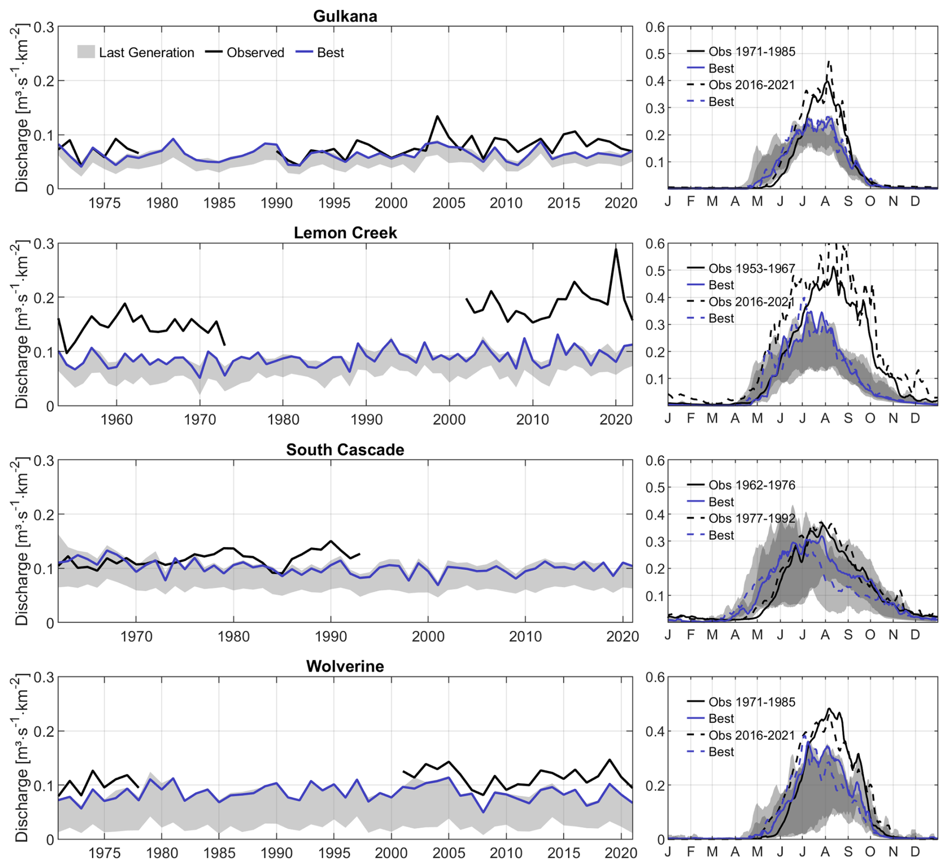
Figure 8Simulation results for cross-validation of the discharge in all four catchments based on mean annual flows (Column 1) and hydrological regimes (Column 2) at the end of the optimization. Hydrological regimes are represented by the mean of daily flows for each day of the year (from day 1 to 366) for the earliest available slice of validation period 1 (solid black line represents the observation, and solid blue line denotes the best simulation; see also Table 2) and the latest available period of validation period 2 (dashed black line represents the observation, and dashed blue line denotes the best simulation). Blue lines (simulation) cover the same period as their black counterparts.
Evaluating the mean daily discharge of the different periods further stresses the substantial undercatch of flow in the simulations (Fig. 8 for all glaciers). The periods were chosen so that they lie apart from each other to highlight potential model deficiencies in the representation of nonstationarities. The LCG and GG models do not show any significant change in the amount of discharge between the early and late periods. This points to relatively stable glacier conditions. In contrast, flows in the SCG basin essentially decrease in the later period, which is in line with the aforementioned results. A similar, albeit not as pronounced, pattern is found for the WG model. The model of the SCG shows the largest range of simulated flows over the year (gray shadings). The share of simulations with a positive mass balance for the WG (see Sect. 3.3) is likely causing the very low simulation bound of discharge in the basin, with almost no flow until August.
3.6 Comparison of SWAT-GL single-objective and multi-objective optimization and the SWAT standard
To illustrate the capabilities of SWAT-GL in terms of discharge and mass balance simulations, two separate SOOs were conducted. The SOO of discharge was evaluated using fKGE, and that of mass balance relied on fNRMSE, ensuring consistency with the MOO counterpart. The results of the two SOO models are compared with the MOO model results introduced and shown in Sects. 3.3–3.5 (using SC, MB and hypsometry). In addition, two SWAT standard models that do not consider glacier processes were created as lower and upper benchmark models. The LB represents the median fKGE of Q for 1000 Latin-hypercube-based simulations. The UB model is optimized for discharge only, analogous to the discharge SOO SWAT-GL model. However, it is also based on SWAT rather than SWAT-GL. The evaluation focuses on the WG only and replicates a typical hydrological modeling case where either discharge or mass balance is the only objective. It is important to note that we are not endorsing this approach as desirable; rather, we highlight that, despite well-known shortcomings of SOO studies, the approach remains a common practice. For the SOO of mass balance, the parameter choices and ranges are similar to Table 3. The introduction aims to improve SWAT-GL's capabilities in the representation of streamflow.
The results are illustrated in Fig. 9. For discharge (a), the SOO results demonstrate a sharp increase in fKGE values when discharge is used directly as the objective, compared to fKGE values from the MOO. The former best fKGE of 0.64 (Table 5) is substituted by a relatively high upper bound of 0.91. The results are reached after only 40 generations and lead to a median fKGE shift from around ∼0.5 to around ∼0.9. In addition, the median fKGE of the MOO corresponds to the lower bound of the Q SOO. Although the simulated mean annual flow of the MOO procedure showed a significant bias compared to the observed flow (see Fig. 8), the SOO Q results in fPBIAS values of −0.78 % (not shown) and is thus capable of bringing reasonable amounts of water into the system. The MOO shows slightly poorer discharge results compared to those resulting from the MB SOO. Below the 20th percentile, the performance of MOO is largely degraded. The SWAT-based UB model only reaches maximum fKGE values below 0.7 and thus significantly below the Q SOO SWAT-GL counterpart. The LB results are even below 0.4, and even the MOO without Q using SWAT-GL is substantially better (in its median), though worse than the SWAT UB. The highest fKGE values from the MB SOO exceed both the LB and UB.
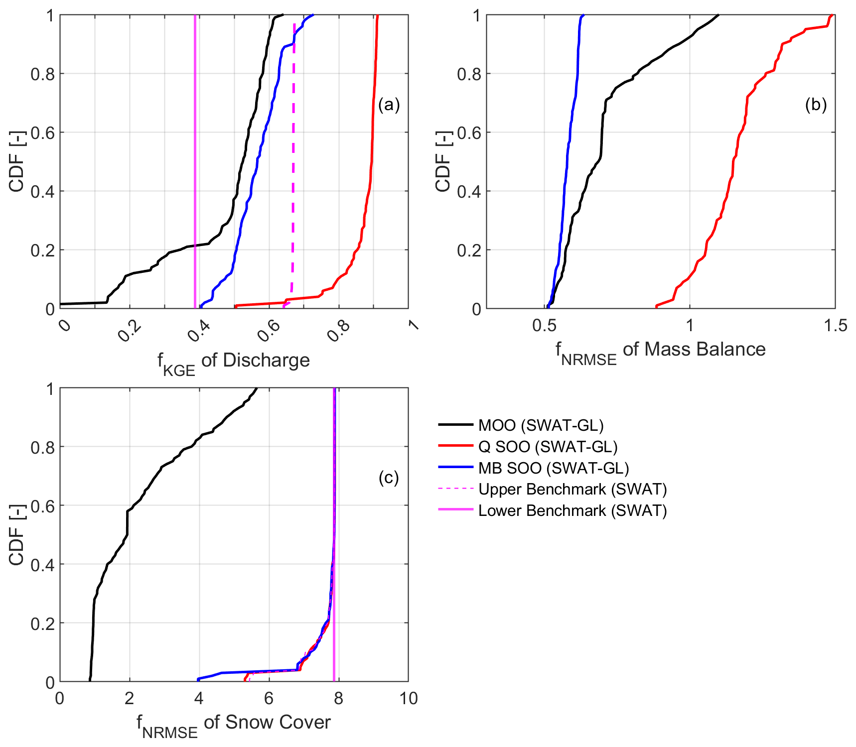
Figure 9Cumulative distribution function (CDF) plots of the objective functions for the different SWAT-GL models (single-objective optimization (SOO) for mass balance and discharge and multi-objective optimization (MOO)) and the lower benchmark (LB) and upper benchmark (UB) SWAT standard models for Wolverine Glacier. (a) shows the results for discharge, (b) for mass balance (note that no LB and UB are provided, as the SWAT standard does not simulate mass balance) and (c) for snow cover. Q SOO refers to the SWAT-GL model optimized for discharge, and MB SOO for the SWAT-GL model optimized for mass balance. The CDF of the MOO refers to the last generation (Generation =100), while the selected SOO results refer to generations up to the convergence point. In detail, the selected generation of the Q SOO and UB model is generation 40, whereas that of the MB SOO model is generation 20. The subscripts “Q” and “MB” indicate discharge and mass balance, respectively. The sample size N of the CDFs is 100, which refers to the general sample size in the optimization. Note that the LB is a vertical line, as it represents only one simulation (median fKGE of Q for 1000 Latin hypercube samples).
The SOO of discharge shows a substantial degradation in representing the annual mass balance compared to the MOO and MB SOO (b). The best solution of the SOO of discharge has a fNRMSE value that is ∼0.37 above the MOO counterpart (or 78 %). Despite a substantially improved MB representation already after 20 generations seen in the MB SOO, the “best” performing simulations (smaller than the 10 % percentile) are similar between MOO and MB SOO. The MB SOO model does not exceed the minimum fNRMSE of 0.51 achieved in the MOO, even after convergence. This result highlights the suitability of an MOO with SWAT-GL for complex glaciated and snow-fed catchments.
When looking at SC, which was not included in the SOO models but was in the MOO, the MOO yields largely superior results. The MB SOO is slightly better in the low percentiles but is generally identical in simulating SC compared to the Q SOO. Also, the LB and UB based on the SWAT standard show nearly identical results for SC as the two SOO models. It is thus notable how the SC results improve drastically even in a MOO framework compared to simulations where SC is not considered. It would be interesting to see whether a SOO using SC only would further improve the results. Furthermore, the comparability, especially for discharge, is constrained because it was not considered in the MOO.
As a profound evaluation of SWAT-GL's performance in different glaciated catchments has been missing so far, the intention was to contribute to the closing of this gap with our work. Note that further information with respect to the technical details of SWAT-GL and future plans about model improvements are found in Schaffhauser et al. (2024).
4.1 Glacier parameterizations and process representation
We used the Morris method to identify (screen) and rank glacier and snow parameters in the four basins (Song et al., 2015; Pianosi et al., 2016; Sarrazin et al., 2016).
In general, lapse rates together with parameters controlling the maximum degree-day factor for ice (and thus glacier melt) were shown to be among the most sensitive parameters in all catchments. The strong temperature-dependence of SWAT-GL is further emphasized by the high sensitivity of the threshold temperature when glacier melt occurs. An important role is played by the SWE threshold, as it determines when a (sub-)basin is fully snow-covered. The parameter links the old snow routine and the newly integrated glacier routine, as glacier melt can occur only under snow-free conditions on the glacier. SWAT's snow cover has received growing attention in multi-objective calibration studies that try to improve model consistency (Tuo et al., 2018; Grusson et al., 2015). The fraction of snow cover directly affects the amount of daily snow melt (lower fractions reduce the amount of snow melt) and indirectly glacier melt. As any degree of snow cover can be achieved with any SWE, there is also the risk of accomplishing good snow cover results with implausible amounts of snow. This circumstance is, contrary to its importance, rarely discussed in the literature. SWE measurements can therefore add significant benefits, as they provide valuable insights into actual amounts of snow. However, resolutions of reanalysis or remote-sensing-based SWE products, along with the significant variability observed in product comparison studies, remain a challenge. SWE observations would be more suitable for drawing conclusions about precipitation inputs compared to relying solely on snow cover. We want to further emphasize that the intermediate sensitivity of precipitation lapse rates might be misleading. The objectives chosen might not be sufficient to allow for precipitation-related conclusions, as none of the three variables are based on absolute volumes (of snow or ice). For example, a separate consideration of summer ablation and winter accumulation would provide a more realistic picture of system inputs and outputs.
As SWAT-GL is still in its early stages, SA was conducted for diagnostic purposes, involving screening and ranking among different catchments. This was done independently of the optimization purpose. In future applications, the dimensions of the parameter space should be reduced accordingly. The SA, for example, suggested a reduction of the parameter space (by six to eight dimensions) in the different catchments of the study. The derived glacier parameter sets after optimization are relatively well-spread in the parameter space. However, in the demonstration catchments, the maximum melt factor tends to group at its defined lower bound. This indicates a potential reduction of the lower bound for an even better representation of glacier mass balance. The chosen values could be reduced, however, as SWAT-GL internally makes a plausibility check between the estimated snow and ice degree-day factors; a further reduction might make internal corrections of the degree-day factor more likely. In addition, further reducing the lower bound of the parameter might exacerbate the strong underestimation of flow. The high values of the glacier melt temperature imply that the models seem to compensate for other temperature-dependent processes, as the model seems to try to delay glacier melt. This indicates that glaciers are, despite the good SC representation, snow-free and exposed to melting too early. A lag factor similar to the temperature lag factor of snow already present in SWAT could also give further control in the timing of glacier melt. However, our study has shown that the snow lag factor is not very sensitive, although its lower bound was chosen to avoid abrupt and extreme snow melt events. We further propose that alternative solutions concerning the lag of ice and snow melt might be explored and evaluated in order to decouple them more clearly from the lag factor related to effective precipitation.
Overall, the standard deviation of the elementary effects indicates that glacier and snow processes behave strongly non-linearly and exhibit potential interacting effects, which we see as a further indication of SWAT-GL's suitability. The moderate interaction ability for SNOCOVMX is considered to be unusual, as it links snow and glacier processes that would suggest higher interaction and/or non-linearity. Future work might focus on time-varying sensitivity analysis (TVSA), such as DYNIA or also using EEs, to obtain further insights into the parameter dominance at different scales and periods over time (Chiogna et al., 2024). Especially in the context of climate impact assessment, insights into a potential loss in model skill due to a reduction in the dominance of (historically working) parameter sets in non-stationary systems become crucial (Wagener, 2022).
4.2 SWAT-GL's performance in representing glaciated catchments
The optimization procedure using NSGA-II for snow cover, glacier hypsometry and glacier mass balance worked well for the highly glaciated catchments, with the exception of the SCG. For the SCG, an abrupt change in the mass balance estimates in the middle of the simulation period causes implausible results. However, snow cover estimates were very good in all catchments, and we highly recommend using snow cover as an objective function for an adequate representation of mountain hydrology when using SWAT-GL. This is particularly true as MODIS (or other) snow cover data are relatively easy to access and widely available, unlike glacier mass balance measurements, which are more challenging to obtain. In data-scarce regions, predominantly the typical setting of high mountainous areas, snow cover, in combination with downstream measured discharge, might often be the only source of data for calibration and validation.
While annual net mass balance was well represented, it was noticed that glacier melt tends to start too early, leading to an extended overlapping period where snow and glacier melt contribute equally to runoff generation. The mass balance estimates are better represented for the bigger glaciers or catchments. However, SWAT-GL was introduced to provide a simple but efficient approach to representing glacier dynamics on multiple scales. While SWAT applications often focus on larger scales compared to the relatively small SCG, more evaluation is necessary regarding the reasons for the bad performance and whether it might be linked to the small spatial scale, something that is especially important to investigate given the overall trend of shrinking glaciers across the world.
As hypsometry measurements were available, they were used in the optimization process. In future work, total glacier area might be a suitable alternative to the individual hypsometry time series. As the Δh-parameterization assumes upper parts of a glacier to be more stable, we conclude that the approach might fail to represent the dynamics of the upper elevation sections at the SCG and LCG, while it seems more appropriate for the WG and GG (see Fig. A4). Using total area changes could therefore improve the representation of the overall MOO, as it would circumvent the attempt to reproduce a pattern SWAT-GL is structurally not able to. Similarly, if individual hypsometry time series are used, one might consider putting less weight on the upper parts of the glacier.
We have shown that, by using discharge as a single objective, as done for the WG, the performance could be substantially ameliorated (fKGE>0.9). Using mass balance in the SOO (again for WG), we have shown that the best solutions of the MOO were comparable to those resulting from the SOO with respect to the achieved fNRMSE values. The statistical results of the mass balance estimates significantly dropped using discharge for SOO and could not compete with the MOO mass balance results. In contrast, the resulting discharge performance from the mass balance SOO was better than the discharge representation of the MOO. Unlike mass balance, discharge was not part of the MOO objectives and partly constrains the interpretability. The benchmarking of the discharge-optimized SWAT-GL model against the SWAT standard illustrated the importance of adequate structural representations in high mountain environments. In addition, the results indicate the limited applicability of the SWAT standard in glaciated catchments even when solely conditioned on discharge.
However, the difficulty in achieving model consistency in highly glaciated and mountainous basins became particularly visible in the LCG basin. The studied glaciers generally have a high contribution to streamflow, as, for example, found in O'Neel et al. (2014) (for GG and WG). Because we consistently overestimate ablation for the LCG, it is initially contradictory that we obtain streamflow underestimations of up to about 50 % (ablation mainly refers to glacier melt). Potential reasons can be manifold. A wrong representation of snow amounts and distribution, despite a good snow cover fit, or an underestimation of liquid precipitation (or a combination of the two) might be potential reasons. Moreover, similar to what is described in O'Neel et al. (2014), the model could also underestimate summer ablation and winter accumulation, both of which govern the mass balance, which would again be related to precipitation. However, it seems that precipitation input might be too low because the LCG meteorological data stem from a remote valley station and the model relies on optimized lapse rates. Precipitation estimates in mountainous catchments can generally be considered as a complex field with large uncertainties that are then reflected in our hydrological models (Evin et al., 2024). Therefore, future modeling work could also try to not only use net mass balance but (if available) also make further use of seasonal mass balance (winter accumulation and summer ablation) derivations in the calibration strategy (Schaefli and Huss, 2011). The winter mass balances could also be used to additionally validate the precipitation inputs from the stations and to adjust the precipitation lapse rates.
In general, it became evident that SWAT-GL is very capable of being applied in glaciated catchments, as well as for longer, non-stationary timescales. It is assumed that the simple degree-day approach integrated in the mass balance module alone could cause significant improvements in glaciated catchments. The simplicity of the approach also leads to high transferability with manageable effort.
4.3 Glacier initialization
A further very sensitive factor that affects the simulation results, in particular under long simulation periods, which are likely subject to persistent climate change effects, is the initialization of the glacier mass. Datasets such as those from Farinotti et al. (2019) or Millan et al. (2022) provide valuable information on glacier thickness and thus mass initialization. However, attention should be paid when simulation periods start decades before the considered thickness estimates. A comparison of the mass differences between the Farinotti estimates and our own calculations based on GlabTop-2 for the earliest possible DEM and outline (see Sect. 2.5) reveals substantial differences. The magnitudes are between −11 % and +19 %. The contradictory signs are produced because the Randolph Glacier Inventory outlines for the different glaciers stem from different acquisition years, which are sometimes earlier than the outlines used for GlabTop-2. This emphasizes the importance of the initialization assumptions. In greater detail, temperature conditions back then might not be suitable to trigger glacier melt at an appropriate magnitude, as lower glacier bounds are simply located too high. Basically, there would be a mismatch between the link of glacier elevation and runoff generation. This becomes evident when examining areal losses as a fraction of the initial area of each glacier over the simulation period (see Appendix A5), where fractional area losses range from more than 10 % (WG) to more than 40 % (SCG).
The Δh approach implemented in SWAT-GL does not consider glacier flow and does allow for glacier area growth (not to be confused with accumulation in the ice water equivalent of a specific ES) in its current version, which is relevant especially for long simulation periods with phases of growth.
The recently extended version of SWAT, called SWAT-GL, was tested in representing the hydrology of four highly glaciated basins. The new SWAT-GL, which makes use of a physical-based glacier evolution routine, has proved to provide robust hydrological simulations of catchments that are characterized by nivo-glacial processes. It thus serves its purpose and adds a valuable contribution to the hydrological modeling community and, in particular, the SWAT community.
We also identified traditional model consistency issues prevalent in hydrological modeling and demonstrated their significance, even when multiple glacier and snow processes are included in the calibration procedure. Although SWAT-GL substantially improves model consistency, such problems should receive more attention. Although we could show SWAT-GL's applicability even under long transient conditions, constraints remain and require further efforts to address. This is particularly true for climate impact studies, where simulation periods can exceed 100 years. In such studies, we advocate a minimum requirement that assesses the suitability of model components for climate impact statements to avoid flawed conclusions. Transient conditions, for example, could significantly affect degree-day factors, making initial choices inappropriate, a topic that is rarely addressed and discussed.
We identified parameter clustering at the edges of the initial parameter ranges, which indicates solutions that could impair physical plausibility. In addition, contradictory patterns were found in the representation of snow and glacier processes (and discharge). For example, a good representation of the snow and glacier processes partly resulted in an unsatisfactory representation of streamflow. We demonstrated that an adequate-to-good snow cover simulation does not necessarily lead to an accurate representation of glacier components. These basic insights, although partly recognized, go beyond SWAT-GL applications and are of general importance for the modeling community. The sensitivity analysis of SWAT-GL showed a strong temperature-dependence of the model. This underpinned the importance and role of lapse rate parameterizations, also as a major source of uncertainty, in high mountainous catchments. However, by benchmarking different SWAT-GL models against the SWAT standard, substantial improvements in representing water availability were highlighted.
Despite SWAT-GL being tested in catchments that are unprecedented in terms of data availability, the authors see no restrictions in its transferability to areas with poor data. Global datasets of ice thickness estimates and glacier outlines set a suitable baseline to apply SWAT-GL. Although relatively small glaciated catchments were employed, the approach can be scaled up without imposing any substantial additional computational demand or physical limitation on the approach.
In conclusion, the most significant merit we discovered with SWAT-GL was its ability to adequately represent glacier processes and outperform the SWAT standard in contrasting glaciated catchments. This encourages its further application and need in high mountainous catchments.
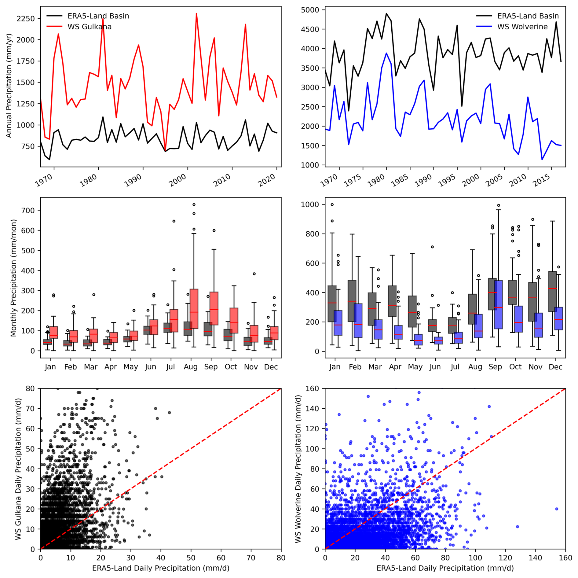
Figure A1Comparison of the used weather station (WS) precipitation data with ERA-Land Reanalysis data for the Wolverine and Gulkana glaciers, as the station data refer to local stations. ERA5-Land results refer to the mean over all pixels that touch the corresponding basin boundary (4 pixels for both basins).
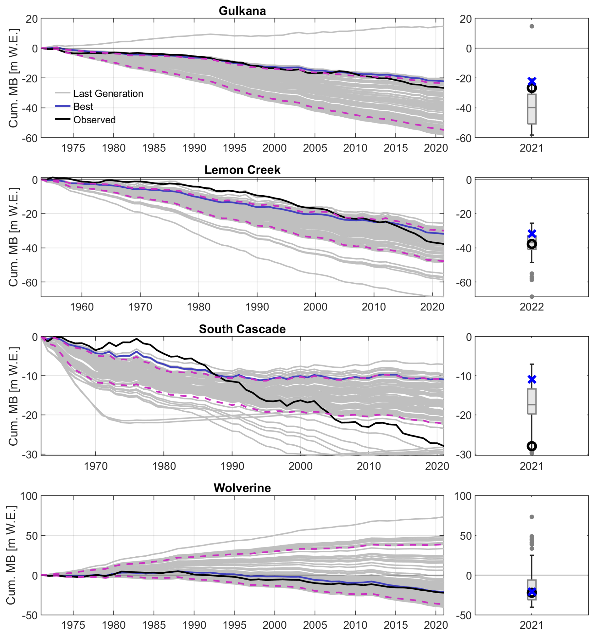
Figure A2Similar to the cumulative mass balance plot of Fig. 7 but providing all individual solutions of the final generation instead of the range. The boxplots provide an estimate of the distribution of the cumulative mass balance at the end of the simulation period. For example, the boxplot of GG consists of the 100 individual cumulative mass balance estimates of year 2021. Blue crosses indicate the results of the best annual mass balance representation in the optimization, and black circles indicate the final observed value. Dashed purple lines refer to the 10th and 90th percentiles.
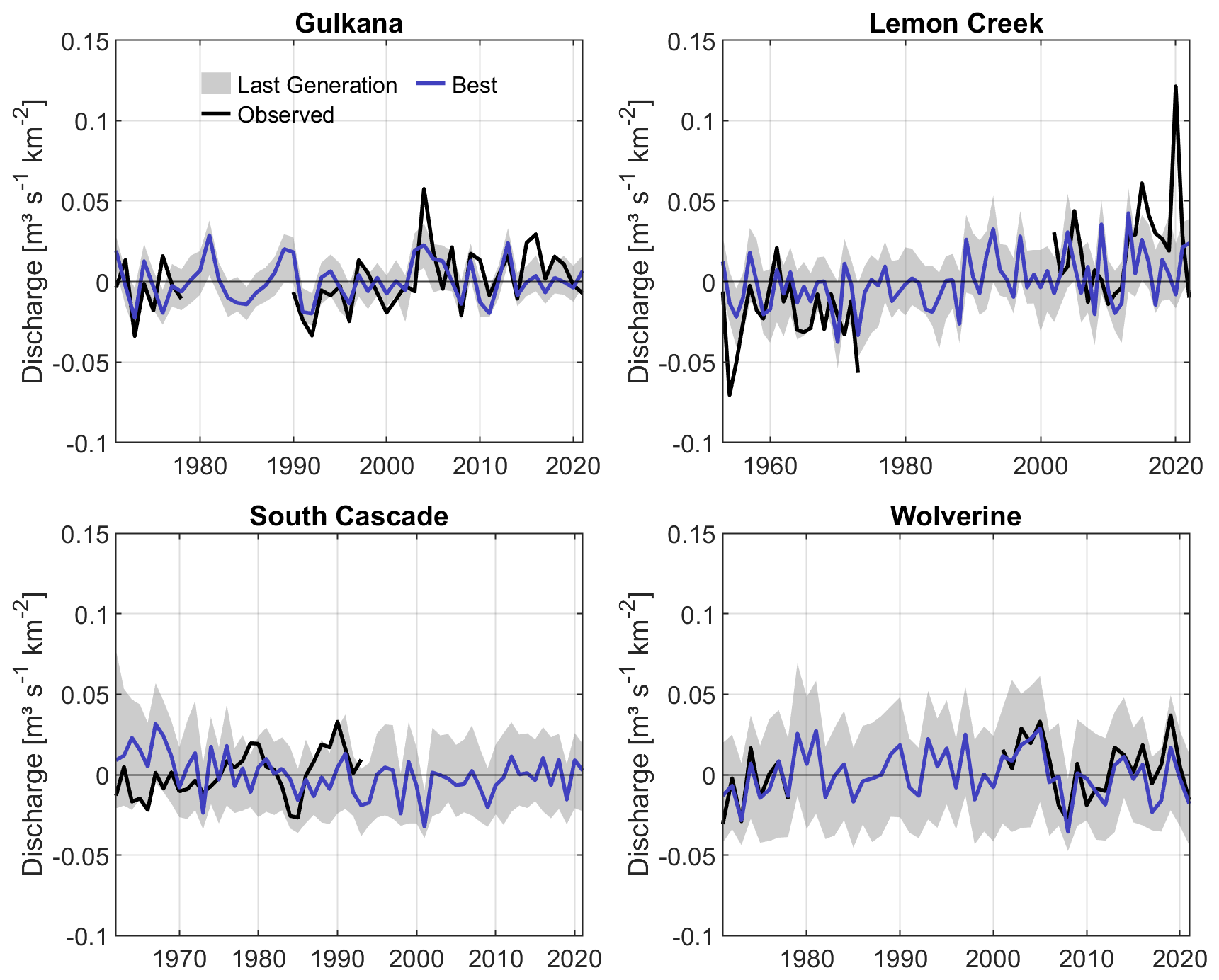
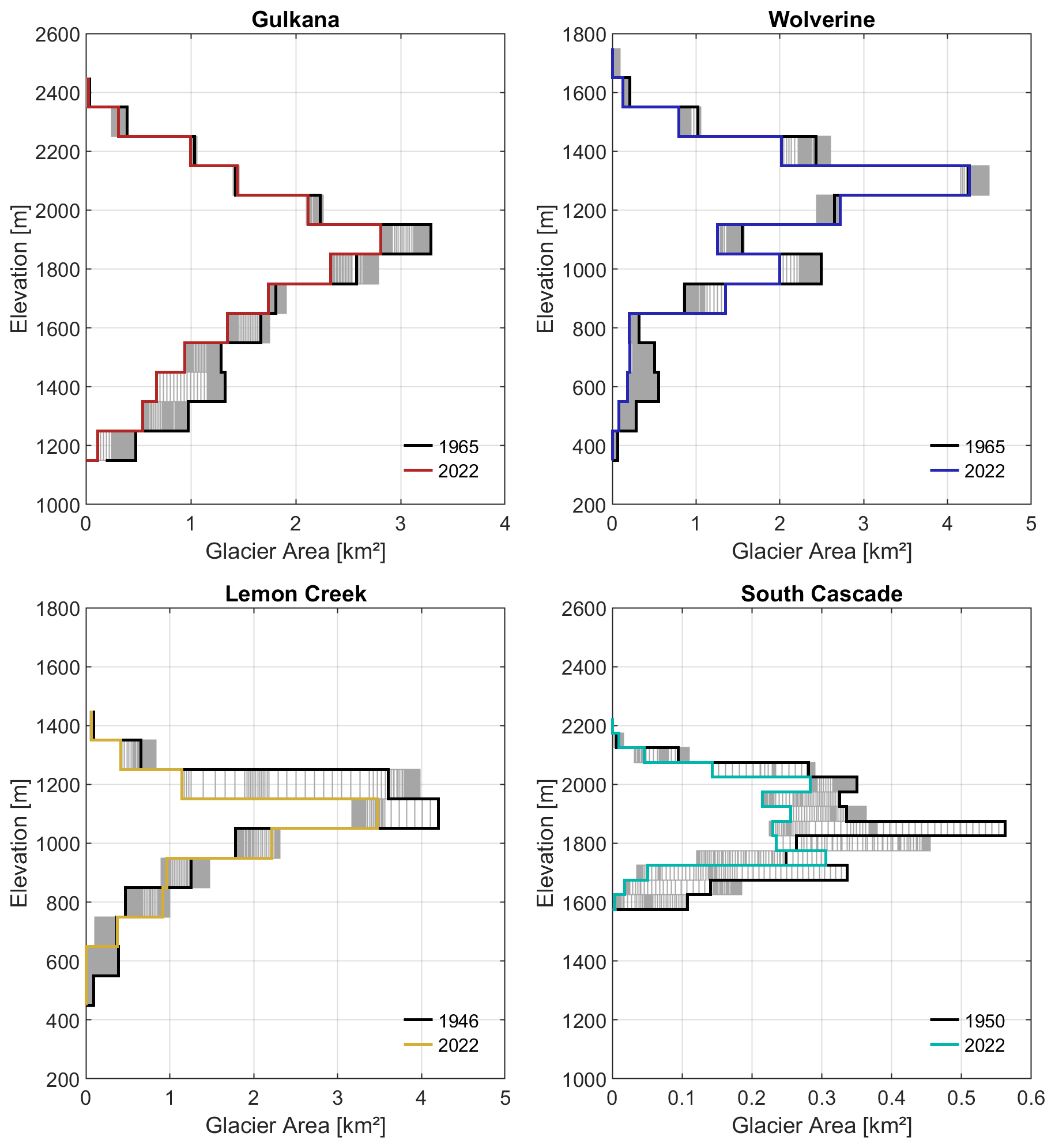
Figure A4Annual glacier hypsometry observations for all four glaciers. Gray indicates each year where the data were available, while black represents the first available year and the individual colors the last available year of measurements.
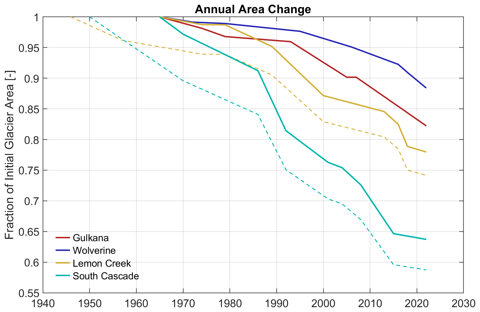
Figure A5Observed annual glacier area observations of all glaciers, expressed as a fraction of the initial area. Solid lines represent the earliest date of overlap between all glaciers, and dashed lines represent the dates on which the mass balance measurement started in case they deviate from the starting point of the solid counterpart (only for SCG and LCG).
Table A1Parameter ranges and median values of all glaciers for the last generation of the optimization. Note: only the glacier parameters are shown here, which is the main novelty and purpose of the article.
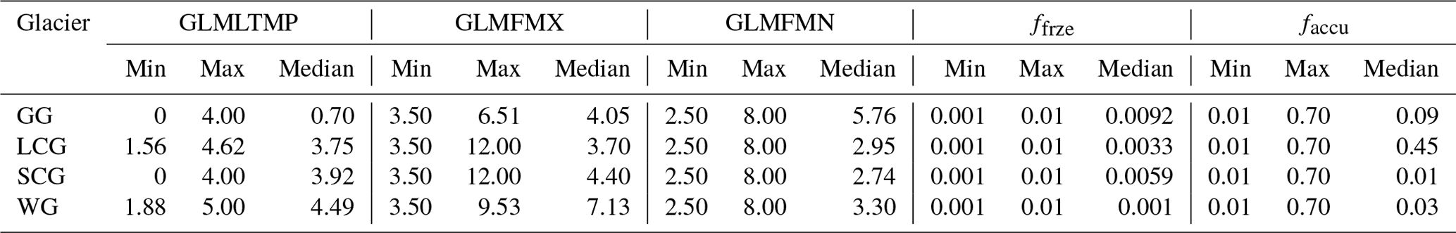
Code and executable of SWAT-GL can be acquired from https://gitlab.com/lshm1/swat-g (https://doi.org/10.5281/zenodo.8068724, Schaffhauser, 2024). The underlying hydrological, meteorological and glaciological data can be obtained from the USGS Benchmark Glacier Project: https://www.usgs.gov/publications/us-geological-survey-benchmark-glacier-project (Florentine and McKeon, 2022).
TS, FM, FH, GC, MD, YT, LA, JM – paper review and editing; TS, FM, MD – study design; TS, FM, JM – data acquisition; TS, FM, FH, JM – data analysis and modeling; TS, FM, FH, GC, MD, YT, LA, JM – model evaluation; TS – paper draft.
The contact author has declared that none of the authors has any competing interests.
Publisher's note: Copernicus Publications remains neutral with regard to jurisdictional claims made in the text, published maps, institutional affiliations, or any other geographical representation in this paper. While Copernicus Publications makes every effort to include appropriate place names, the final responsibility lies with the authors.
We gratefully acknowledge support from the United States Geological Survey (USGS) Benchmark Glacier Project for providing the comprehensive datasets. The authors also want to thank Scott Boyce from USGS for assisting the work.
This research has been supported by the Bundesministerium für Bildung und Forschung (grant no. 01LZ1802B) and by the EU Horizon Europe project WE-ACT (ID 101083481).
This paper was edited by Jan Seibert and reviewed by Cyril Thébault, Dipti Tiwari, and one anonymous referee.
Adnan, M., Kang, S., Zhang, G., Saifullah, M., Anjum, M. N., and Ali, A. F.: Simulation and analysis of the water balance of the Nam Co Lake using SWAT model, Water-Sui., 11, 1383, https://doi.org/10.3390/w11071383, 2019. a
Ali, S. H., Bano, I., Kayastha, R. B., and Shrestha, A.: COMPARATIVE ASSESSMENT OF RUNOFF AND ITS COMPONENTS IN TWO CATCHMENTS OF UPPER INDUS BASIN BY USING A SEMI DISTRIBUTED GLACIO-HYDROLOGICAL MODEL, Int. Arch. Photogramm. Remote Sens. Spatial Inf. Sci., XLII-2/W7, 1487–1494, https://doi.org/10.5194/isprs-archives-XLII-2-W7-1487-2017, 2017. a
Arnold, J. G., Srinivasan, R., Muttiah, R. S., and Williams, J. R.: Large area hydrologic modeling and assessment part I: Model development, J. Am. Water Resour. As., 34, 73–89, https://doi.org/10.1111/j.1752-1688.1998.tb05961.x, 1998. a
Bahr, D. B., Pfeffer, W. T., and Kaser, G.: A review of volume-area scaling of glaciers, Rev. Geophys., 53, 95–140, https://doi.org/10.1002/2014rg000470, 2015. a
Baker, E. H., Mcneil, C. J., Sass, L., Peitzsch, E. H., Whorton, E. N., Florentine, C. E., Clark, A. M., Miller, Z. S., Fagre, D. B., and O'Neel, S. R.: USGS Benchmark Glacier Mass Balance and Project Data, United States Geological Survey (USGS) [data set], https://doi.org/10.5066/F7BG2N8R, 2018. a, b
Campolongo, F., Saltelli, A., and Cariboni, J.: From screening to quantitative sensitivity analysis. A unified approach, Comput. Phys. Commun., 182, 978–988, https://doi.org/10.1016/j.cpc.2010.12.039, 2011. a, b
Chen, Y., Li, W., Fang, G., and Li, Z.: Review article: Hydrological modeling in glacierized catchments of central Asia – status and challenges, Hydrol. Earth Syst. Sci., 21, 669–684, https://doi.org/10.5194/hess-21-669-2017, 2017. a
Chiogna, G., Marcolini, G., Engel, M., and Wohlmuth, B.: Sensitivity analysis in the wavelet domain: a comparison study, Stoch. Env. Res. Risk. A., 38, 1669–1684, https://doi.org/10.1007/s00477-023-02654-3, 2024. a
Dawar, D. and Ludwig, S.: Differential evolution with dither and annealed scale factor, in: 2014 IEEE Symposium on Differential Evolution (SDE), IEEE, Orlando, FL, USA, 9–12 December 2014, 1–8, https://doi.org/10.1109/sde.2014.7031528, 2014. a
Deb, K., Pratap, A., Agarwal, S., and Meyarivan, T.: A fast and elitist multiobjective genetic algorithm: NSGA-II, IEEE T. Evolut. Comput., 6, 182–197, https://doi.org/10.1109/4235.996017, 2002. a
Dozier, J.: Spectral signature of alpine snow cover from the landsat thematic mapper, Remote Sens. Environ., 28, 9–22, https://doi.org/10.1016/0034-4257(89)90101-6, 1989. a
Du, X., Silwal, G., and Faramarzi, M.: Investigating the impacts of glacier melt on stream temperature in a cold-region watershed: coupling a glacier melt model with a hydrological model, J. Hydrol., 605, 127303, https://doi.org/10.1016/j.jhydrol.2021.127303, 2022. a
Evin, G., Le Lay, M., Fouchier, C., Penot, D., Colleoni, F., Mas, A., Garambois, P.-A., and Laurantin, O.: Evaluation of hydrological models on small mountainous catchments: impact of the meteorological forcings, Hydrol. Earth Syst. Sci., 28, 261–281, https://doi.org/10.5194/hess-28-261-2024, 2024. a
Farinotti, D., Huss, M., Fürst, J. J., Landmann, J., Machguth, H., Maussion, F., and Pandit, A.: A consensus estimate for the ice thickness distribution of all glaciers on Earth, Nat. Geosci., 12, 168–173, https://doi.org/10.1038/s41561-019-0300-3, 2019. a, b, c
Frey, H., Machguth, H., Huss, M., Huggel, C., Bajracharya, S., Bolch, T., Kulkarni, A., Linsbauer, A., Salzmann, N., and Stoffel, M.: Estimating the volume of glaciers in the Himalayan–Karakoram region using different methods, The Cryosphere, 8, 2313–2333, https://doi.org/10.5194/tc-8-2313-2014, 2014. a
Florentine, C. and McKeon, L. A.: U.S. Geological Survey Benchmark Glacier Project: U.S. Geological Survey Fact Sheet 2022-3050, 2 pp., https://www.usgs.gov/publications/us-geological-survey-benchmark-glacier-project (last access: 1 April 2024), 2022. a
Gan, R., Luo, Y., Zuo, Q., and Sun, L.: Effects of projected climate change on the glacier and runoff generation in the Naryn River Basin, Central Asia, J. Hydrol., 523, 240–251, https://doi.org/10.1016/j.jhydrol.2015.01.057, 2015. a
Garcia Sanchez, D., Lacarrière, B., Musy, M., and Bourges, B.: Application of sensitivity analysis in building energy simulations: combining first- and second-order elementary effects methods, Energ. Buildings, 68, 741–750, https://doi.org/10.1016/j.enbuild.2012.08.048, 2014. a, b, c
Grusson, Y., Sun, X., Gascoin, S., Sauvage, S., Raghavan, S., Anctil, F., and Sáchez-Pérez, J.-M.: Assessing the capability of the SWAT model to simulate snow, snow melt and streamflow dynamics over an alpine watershed, J. Hydrol., 531, 574–588, https://doi.org/10.1016/j.jhydrol.2015.10.070, 2015. a
Hamed, K. H. and Ramachandra Rao, A.: A modified Mann-Kendall trend test for autocorrelated data, J. Hydrol., 204, 182–196, https://doi.org/10.1016/s0022-1694(97)00125-x, 1998. a, b
Hassan, J., qing Chen, X., Kayastha, R. B., and Nie, Y.: Multi-model assessment of glacio-hydrological changes in central Karakoram, Pakistan, J. Mt. Sci., 18, 1995–2011, https://doi.org/10.1007/s11629-021-6748-9, 2021. a
Hofmeister, F., Arias-Rodriguez, L. F., Premier, V., Marin, C., Notarnicola, C., Disse, M., and Chiogna, G.: Intercomparison of Sentinel-2 and modelled snow cover maps in a high-elevation Alpine catchment, J. Hydrol., 15, 100123, https://doi.org/10.1016/j.hydroa.2022.100123, 2022. a
Horlings, A.: A Numerical Modeling Investigation on Calving and the Recession of South Cascade Glacier, University Honors Theses, Paper 247, https://doi.org/10.15760/honors.307, 2016. a
Huss, M. and Hock, R.: A new model for global glacier change and sea-level rise, Front. Earth Sci., 3, 54, https://doi.org/10.3389/feart.2015.00054, 2015. a
Huss, M., Farinotti, D., Bauder, A., and Funk, M.: Modelling runoff from highly glacierized alpine drainage basins in a changing climate, Hydrol. Process., 22, 3888–3902, https://doi.org/10.1002/hyp.7055, 2008. a, b
Huss, M., Jouvet, G., Farinotti, D., and Bauder, A.: Future high-mountain hydrology: a new parameterization of glacier retreat, Hydrol. Earth Syst. Sci., 14, 815–829, https://doi.org/10.5194/hess-14-815-2010, 2010. a, b, c, d, e, f, g
Ji, H., Fang, G., Yang, J., and Chen, Y.: Multi-objective calibration of a distributed hydrological model in a highly glacierized watershed in Central Asia, Water-Sui., 11, 554, https://doi.org/10.3390/w11030554, 2019. a
Li, H., Beldring, S., Xu, C.-Y., Huss, M., Melvold, K., and Jain, S. K.: Integrating a glacier retreat model into a hydrological model – case studies of three glacierised catchments in Norway and Himalayan region, J. Hydrol., 527, 656–667, https://doi.org/10.1016/j.jhydrol.2015.05.017, 2015. a, b
Linsbauer, A., Paul, F., and Haeberli, W.: Modeling glacier thickness distribution and bed topography over entire mountain ranges with GlabTop: application of a fast and robust approach, J. Geophys. Res.-Earth, 117, F03007, https://doi.org/10.1029/2011jf002313, 2012. a
Linsbauer, A, Paul, F, Hoelzle, M, Frey, H, and Haeberli, W: The Swiss Alps without glaciers – a GIS-based modelling approach for reconstruction of glacier beds, Department of Geography, University of Zurich, https://doi.org/10.5167/UZH-27834, 2009. a
Luo, Y., Arnold, J., Liu, S., Wang, X., and Chen, X.: Inclusion of glacier processes for distributed hydrological modeling at basin scale with application to a watershed in Tianshan Mountains, northwest China, J. Hydrol., 477, 72–85, https://doi.org/10.1016/j.jhydrol.2012.11.005, 2013. a
Luo, Y., Wang, X., Piao, S., Sun, L., Ciais, P., Zhang, Y., Ma, C., Gan, R., and He, C.: Contrasting streamflow regimes induced by melting glaciers across the Tien Shan – Pamir – North Karakoram, Sci. Rep., 8, 16470, https://doi.org/10.1038/s41598-018-34829-2, 2018. a
Ma, C., Sun, L., Liu, S., Shao, M., and Luo, Y.: Impact of climate change on the streamflow in the glacierized Chu River Basin, Central Asia, J. Arid Land., 7, 501–513, https://doi.org/10.1007/s40333-015-0041-0, 2015. a
Mcneil, C. J., Sass, L., Florentine, C., Baker, E. H., Peitzsch, E. H., Whorton, E. N., Miller, Z., Fagre, D. B., Clark, A. M., and O'Neel, S. R.: Glacier-Wide Mass Balance and Compiled Data Inputs: USGS Benchmark Glaciers, Alaska Science Center [data set], https://doi.org/10.5066/F7HD7SRF, 2016. a, b
Merchán-Rivera, P., Geist, A., Disse, M., Huang, J., and Chiogna, G.: A Bayesian framework to assess and create risk maps of groundwater flooding, J. Hydrol., 610, 127797, https://doi.org/10.1016/j.jhydrol.2022.127797, 2022. a, b
Merk, F., Schaffhauser, T., Anwar, F., Tuo, Y., Cohard, J.-M., and Disse, M.: The significance of the leaf area index for evapotranspiration estimation in SWAT-T for characteristic land cover types of West Africa, Hydrol. Earth Syst. Sci., 28, 5511–5539, https://doi.org/10.5194/hess-28-5511-2024, 2024. a
Millan, R., Mouginot, J., Rabatel, A., and Morlighem, M.: Ice velocity and thickness of the world's glaciers, Nat. Geosci., 15, 124–129, https://doi.org/10.1038/s41561-021-00885-z, 2022. a, b
Moriasi, D. N., Arnold, J. G., Liew, M. W. V., Bingner, R. L., Harmel, R. D., and Veith, T. L.: Model evaluation guidelines for systematic quantification of accuracy in watershed simulations, T. ASABE, 50, 885–900, https://doi.org/10.13031/2013.23153, 2007. a
Morris, M. D.: Factorial sampling plans for preliminary computational experiments, Technometrics, 33, 161–174, https://doi.org/10.1080/00401706.1991.10484804, 1991. a, b
Moriasi, N. D., Gitau, W. M., Pai, N., and Daggupati, P.: Hydrologic and water quality models: performance measures and evaluation criteria, T. ASABE, 58, 1763–1785, 2015. a
Muñoz Sabater, J.: ERA5-Land hourly data from 1950 to present, Copernicus Climate Change Service (C3S) Climate Data Store (CDS) [data set], https://doi.org/10.24381/cds.e2161bac, 2019. a
NASA JPL: NASA Shuttle Radar Topography Mission Global 1 arc second, NASA Land Processes Distributed Active Archive Center [data set], https://doi.org/10.5067/MEASURES/SRTM/SRTMGL1.003, 2013. a
Naz, B. S., Frans, C. D., Clarke, G. K. C., Burns, P., and Lettenmaier, D. P.: Modeling the effect of glacier recession on streamflow response using a coupled glacio-hydrological model, Hydrol. Earth Syst. Sci., 18, 787–802, https://doi.org/10.5194/hess-18-787-2014, 2014. a, b
Nossent, J., Elsen, P., and Bauwens, W.: Sobol' sensitivity analysis of a complex environmental model, Environ. Modell. Softw., 26, 1515–1525, https://doi.org/10.1016/j.envsoft.2011.08.010, 2011. a
O'Neel, S., Hood, E., Arendt, A., and Sass, L.: Assessing streamflow sensitivity to variations in glacier mass balance, Climatic Change, 123, 329–341, https://doi.org/10.1007/s10584-013-1042-7, 2014. a, b, c, d, e
O'Neel, S., McNeil, C., Sass, L. C., Florentine, C., Baker, E. H., Peitzsch, E., McGrath, D., Fountain, A. G., and Fagre, D.: Reanalysis of the US Geological Survey Benchmark Glaciers: long-term insight into climate forcing of glacier mass balance, J. Glaciol., 65, 850–866, https://doi.org/10.1017/jog.2019.66, 2019. a, b, c, d, e, f, g, h, i, j, k, l, m, n, o
Pesci, M. H., Schulte Overberg, P., Bosshard, T., and Förster, K.: From global glacier modeling to catchment hydrology: bridging the gap with the WaSiM-OGGM coupling scheme, Frontiers in Water, 5, 1296344, https://doi.org/10.3389/frwa.2023.1296344, 2023. a
Pettitt, A. N.: A Non-Parametric Approach to the Change-Point Problem, Appl. Stat.-J. Roy. St. C, 28, 126, https://doi.org/10.2307/2346729, 1979. a
Pianosi, F., Beven, K., Freer, J., Hall, J. W., Rougier, J., Stephenson, D. B., and Wagener, T.: Sensitivity analysis of environmental models: a systematic review with practical workflow, Environ. Modell. Softw., 79, 214–232, https://doi.org/10.1016/j.envsoft.2016.02.008, 2016. a, b, c
Pradhananga, N. S., Kayastha, R. B., Bhattarai, B. C., Adhikari, T. R., Pradhan, S. C., Devkota, L. P., Shrestha, A. B., and Mool, P. K.: Estimation of discharge from Langtang River basin, Rasuwa, Nepal, using a glacio-hydrological model, Ann. Glaciol., 55, 223–230, https://doi.org/10.3189/2014aog66a123, 2014. a
RGI Consortium: Randolph Glacier Inventory – A Dataset of Global Glacier Outlines, Version 6, National Snow and Ice Data Center [data set], https://doi.org/10.7265/4M1F-GD79, 2017. a, b, c
Saltelli, A., Ratto, M., Andres, T., Campolongo, F., Cariboni, J., Gatelli, D., Saisana, M., and Tarantola, S.: Global Sensitivity Analysis: The Primer, John Wiley and Sons, Print ISBN 9780470059975, online ISBN 9780470725184, https://doi.org/10.1002/9780470725184, 2008. a, b
Sarrazin, F., Pianosi, F., and Wagener, T.: Global sensitivity analysis of environmental models: convergence and validation, Environ. Modell. Softw., 79, 135–152, https://doi.org/10.1016/j.envsoft.2016.02.005, 2016. a, b
Schaefli, B. and Huss, M.: Integrating point glacier mass balance observations into hydrologic model identification, Hydrol. Earth Syst. Sci., 15, 1227–1241, https://doi.org/10.5194/hess-15-1227-2011, 2011. a
Schaffhauser, T.: SWAT-GL Demo Model Martelltal, Zenodo [data set], https://doi.org/10.5281/zenodo.8068724, 2024. a
Schaffhauser, T., Tuo, Y., Hofmeister, F., Chiogna, G., Huang, J., Merk, F., and Disse, M.: SWAT GL: a new glacier routine for the hydrological model SWAT, J. Am. Water Resour. As., 60, 755–766, https://doi.org/10.1111/1752-1688.13199, 2024. a, b, c, d, e, f
Seibert, J., Vis, M. J. P., Kohn, I., Weiler, M., and Stahl, K.: Technical note: Representing glacier geometry changes in a semi-distributed hydrological model, Hydrol. Earth Syst. Sci., 22, 2211–2224, https://doi.org/10.5194/hess-22-2211-2018, 2018. a, b, c
Shafeeque, M., Luo, Y., Wang, X., and Sun, L.: Altitudinal distribution of meltwater and its effects on glacio-hydrology in glacierized catchments, Central Asia, J. Am. Water Resour. As., 56, 30–52, https://doi.org/10.1111/1752-1688.12805, 2019. a
Shannon, S., Payne, A., Freer, J., Coxon, G., Kauzlaric, M., Kriegel, D., and Harrison, S.: A snow and glacier hydrological model for large catchments – case study for the Naryn River, central Asia, Hydrol. Earth Syst. Sci., 27, 453–480, https://doi.org/10.5194/hess-27-453-2023, 2023. a
Sin, G. and Gernaey, K. V.: Improving the Morris method for sensitivity analysis by scaling the elementary effects, in: Computer Aided Chemical Engineering, Elsevier, https://doi.org/10.1016/s1570-7946(09)70154-3, 925–930, 2009. a
Song, X., Zhang, J., Zhan, C., Xuan, Y., Ye, M., and Xu, C.: Global sensitivity analysis in hydrological modeling: review of concepts, methods, theoretical framework, and applications, J. Hydrol., 523, 739–757, https://doi.org/10.1016/j.jhydrol.2015.02.013, 2015. a
Stoll, E., Hanzer, F., Oesterle, F., Nemec, J., Schöber, J., Huttenlau, M., and Förster, K.: What can we learn from comparing glacio-hydrological models?, Atmosphere-Basel, 11, 981, https://doi.org/10.3390/atmos11090981, 2020. a
Storn, R. and Price, K.: Differential Evolution – A Simple and Efficient Heuristic for global Optimization over Continuous Spaces, J. Global Optim., 11, 341–359, https://doi.org/10.1023/a:1008202821328, 1997. a
Tebaldi, C., Debeire, K., Eyring, V., Fischer, E., Fyfe, J., Friedlingstein, P., Knutti, R., Lowe, J., O'Neill, B., Sanderson, B., van Vuuren, D., Riahi, K., Meinshausen, M., Nicholls, Z., Tokarska, K. B., Hurtt, G., Kriegler, E., Lamarque, J.-F., Meehl, G., Moss, R., Bauer, S. E., Boucher, O., Brovkin, V., Byun, Y.-H., Dix, M., Gualdi, S., Guo, H., John, J. G., Kharin, S., Kim, Y., Koshiro, T., Ma, L., Olivié, D., Panickal, S., Qiao, F., Rong, X., Rosenbloom, N., Schupfner, M., Séférian, R., Sellar, A., Semmler, T., Shi, X., Song, Z., Steger, C., Stouffer, R., Swart, N., Tachiiri, K., Tang, Q., Tatebe, H., Voldoire, A., Volodin, E., Wyser, K., Xin, X., Yang, S., Yu, Y., and Ziehn, T.: Climate model projections from the Scenario Model Intercomparison Project (ScenarioMIP) of CMIP6, Earth Syst. Dynam., 12, 253–293, https://doi.org/10.5194/esd-12-253-2021, 2021. a
Tiel, M., Stahl, K., Freudiger, D., and Seibert, J.: Glacio-hydrological model calibration and evaluation, WIREs Water, 7, e1483, https://doi.org/10.1002/wat2.1483, 2020. a, b
Tuo, Y., Duan, Z., Disse, M., and Chiogna, G.: Evaluation of precipitation input for SWAT modeling in Alpine catchment: a case study in the Adige river basin (Italy), Sci. Total Environ., 573, 66–82, https://doi.org/10.1016/j.scitotenv.2016.08.034, 2016. a
Tuo, Y., Marcolini, G., Disse, M., and Chiogna, G.: A multi-objective approach to improve SWAT model calibration in alpine catchments, J. Hydrol., 559, 347–360, https://doi.org/10.1016/j.jhydrol.2018.02.055, 2018. a
U.S. Geological Survey: USGS Water Data for the Nation, U.S. Geological Survey, National Water Information System (NWIS) [data set], https://doi.org/10.5066/F7P55KJN, 1994. a
Vanuytrecht, E., Raes, D., and Willems, P.: Global sensitivity analysis of yield output from the water productivity model, Environ. Modell. Softw., 51, 323–332, https://doi.org/10.1016/j.envsoft.2013.10.017, 2014. a
Wagener, T.: On the Evaluation of Climate Change Impact Models for Adaptation Decisions, Springer International Publishing, 33–40, https://doi.org/10.1007/978-3-030-86211-4_5, 2022. a
Wang, X., Zhang, Y., Luo, Y., Sun, L., and Shafeeque, M.: Combined use of volume-area and volume-length scaling relationships in glacio-hydrological simulation, Hydrol. Res., 49, 1753–1772, https://doi.org/10.2166/nh.2018.137, 2018. a
Wiersma, P., Aerts, J., Zekollari, H., Hrachowitz, M., Drost, N., Huss, M., Sutanudjaja, E. H., and Hut, R.: Coupling a global glacier model to a global hydrological model prevents underestimation of glacier runoff, Hydrol. Earth Syst. Sci., 26, 5971–5986, https://doi.org/10.5194/hess-26-5971-2022, 2022. a
Wilcoxon, F.: Individual comparisons by ranking methods, Biometrics Bull., 1, 80, https://doi.org/10.2307/3001968, 1945. a
Wortmann, M., Bolch, T., Krysanova, V., and Buda, S.: Bridging glacier and river catchment scales: an efficient representation of glacier dynamics in a hydrological model, Hydrol. Earth Syst. Sci. Discuss. [preprint], https://doi.org/10.5194/hess-2016-272, 2016. a, b
Wu, F., Zhan, J., Wang, Z., and Zhang, Q.: Streamflow variation due to glacier melting and climate change in upstream Heihe River Basin, Northwest China, Phys. Chem. Earth, Parts A/B/C, 79–82, 11–19, https://doi.org/10.1016/j.pce.2014.08.002, 2015. a
Yang, C., Xu, M., Fu, C., Kang, S., and Luo, Y.: The coupling of glacier melt module in SWAT model based on multi-source remote sensing data: a case study in the Upper Yarkant River Basin, Remote Sens.-Basel, 14, 6080, https://doi.org/10.3390/rs14236080, 2022. a
Zekollari, H., Huss, M., Farinotti, D., and Lhermitte, S.: Ice dynamical glacier evolution modeling – a review, Rev. Geophys., 60, e2021RG000754, https://doi.org/10.1029/2021rg000754, 2022. a