Representation of a two-way coupled irrigation system in the Common Land Model

Human land–water management, especially irrigation water withdrawal and use, significantly impacts the global and regional water cycle, energy budget, and near-surface climate. While land surface models are widely used to explore and predict the impacts of irrigation, the irrigation system representation in these models is still in its early stages. This study enhances the Common Land Model (CoLM) by introducing a two-way coupled irrigation module. This module includes an irrigation water demand scheme based on soil moisture deficit, an irrigation application scheme considering four major irrigation methods, and an irrigation water withdrawal scheme that incorporates multiple water source constraints by integrating CoLM with a river routing model and a reservoir operation scheme. Crucially, it explicitly accounts for the feedback between irrigation water demand and supply, which is constrained by available surface water (i.e., runoff, streamflow, reservoir storage) and groundwater. Simulations conducted from 2001 to 2016 at a 0.25° spatial resolution across the contiguous United States reveal that the model effectively reproduces irrigation withdrawals, their spatial distribution, and water source proportions, aligning well with reported state-level statistics. Comprehensive validation demonstrates that the new module significantly improves model accuracy in simulating regional energy dynamics (sensible heat, latent heat, and surface temperature), hydrology (river flow), and agricultural outputs (yields for maize, soybean, and wheat). Application analyses highlight the potential of the enhanced CoLM as a valuable tool for predicting irrigation-driven climate impacts and assessing water use and scarcity. This research offers a pathway for a more holistic representation of fluxes in irrigated areas and human–water interactions within land surface models. It is valuable for exploring the interconnected evolution of climate, water resources, agricultural production, and irrigation activities, while supporting sustainable water management decisions in a changing climate.

1 Introduction

Freshwater resources are indispensable for human society. Since 1900, the global population has increased more than 4-fold, leading to a nearly 6-fold rise in water withdrawals, from approximately 500 km³ yr⁻¹ in 1900 to about 3000 km³ yr⁻¹ in 2000, with agriculture being the dominant water user (Pokhrel et al., 2016). Around 70 % of global freshwater has been withdrawn for irrigation (Campbell et al., 2017), accounting for 90 % of consumptive water use (Siebert and Döll, 2010), with irrigated areas providing approximately 40 % of global food production on just 2.5 % of global land (bin Abdullah, 2006). Accompanied by significant socioeconomic benefits, these intense human land–water management practices have profoundly altered Earth's surface and impacted terrestrial water and energy cycles (Ketchum et al., 2023; Nocco et al., 2019; Rappin et al., 2022; Thiery et al., 2017; de Vrese et al., 2016). The demand for irrigation water is anticipated to rise with the growing global population and food demand, while climate-warming-induced droughts are likely to exacerbate this need (McDermid et al., 2023; Mehta et al., 2024; Yang et al., 2023). Therefore, understanding and quantifying the impacts of irrigation water management in human–Earth system interactions are crucial for developing strategies to sustainably manage these resources amidst changing climatic and demographic conditions.

Irrigation practices transfer water from various sources, such as rivers, lakes, reservoirs, and aquifers, into agricultural systems, directly affecting the magnitude and timing of runoff and river flow (Ketchum et al., 2023). The rising irrigation demand has spurred increased construction of reservoirs and diversions, resulting in both local and downstream impacts. In some regions, water extraction for irrigation has reduced the availability of both surface and groundwater (Döll et al., 2014). Besides modifying water fluxes, irrigation also influences regional climates both locally and remotely. Locally, it alters surface albedo, evapotranspiration, and surface soil moisture, impacting regional radiation and energy balances and affecting temperature, humidity, and precipitation through land–atmosphere feedback (Chen and Dirmeyer, 2019; Kang and Eltahir, 2018; Li et al., 2022; McDermid et al., 2017; Nocco et al., 2019). Remotely, it affects climate through complex interactions between altered temperature and moisture gradients and larger-scale processes such as atmospheric circulation and wave activity (Douglas et al., 2009; Phillips et al., 2022; de Vrese et al., 2016).

Earth system models (ESMs) are powerful tools for examining the interactions and feedback among the intricately intertwined processes of the Earth system, both in the past and future. Land surface models (LSMs) are a crucial component of ESMs. Due to the complex dynamics of natural hydrological processes and anthropogenic activities, describing human–water interactions has been recognized as a significant challenge in land surface modeling (Nazemi and Wheater, 2015). In recent years, targeted efforts have aimed to address this deficiency, yet water use remains largely underrepresented or in a nascent stage within LSMs (Blyth et al., 2021; Taranu et al., 2024). Meanwhile, global hydrological models (GHMs), originally designed for water resource assessment, have undergone continuous improvements over the last 3 decades to explicitly represent human water use (Hanasaki et al., 2018; Liang et al., 1994; Müller Schmied et al., 2021; Sood and Smakhtin, 2015; Sutanudjaja et al., 2018; Tang et al., 2007). These models enable the determination of the spatial distribution and temporal evolution of water resources and water stress for both humans and other biota under the pressures of global change (Döll et al., 2018; Schewe et al., 2014; Schlosser et al., 2014). These advancements have offered valuable insights for incorporating human water use into LSMs.

Parameterizing irrigation water use and modeling its impacts in GHMs and LSMs has been approached using different assumptions and simplifications in three key aspects: irrigation demands, irrigation methods, and irrigation water supplies/withdrawals. The first aspect is estimating irrigation water demands. Models estimate these demands using either a root-zone soil moisture deficit approach or a crop-specific potential evapotranspiration approach. The root-zone soil moisture deficit approach estimates irrigation demand as the water needed to keep root-zone soil moisture (usually within the top meter of soil) above a certain threshold during the growing season (normally a certain percentage of field capacity or soil saturation) (Ozdogan et al., 2010). The crop-specific potential evapotranspiration approach estimates irrigation needs based on the difference between crop-specific potential evapotranspiration and simulated unirrigated evapotranspiration, or between potential and effective precipitation under well-watered conditions where crops transpire at their maximum rate (Müller Schmied et al., 2021). Notably, LSMs generally do not use potential evapotranspiration to estimate irrigation demand.

The second aspect concerns the representation of irrigation methods. Many models simplify irrigation application by directly modifying soil moisture or treating it as additional rainfall across all irrigated land, overlooking the diversity of irrigation techniques employed in various parts of the world or by different farmers (Li et al., 2024a; Lu et al., 2015; de Vrese et al., 2018). Recently, some models have started integrating specific irrigation techniques for certain crops or regions. For instance, LPJmL includes sprinkler, drip, and surface irrigation methods, and CLM incorporates drip, sprinkler, flood, and paddy irrigation methods (Jägermeyr et al., 2015; Yao et al., 2022). Different irrigation techniques affect farmland hydrological processes and irrigation efficiency in distinct ways. For example, drip and surface irrigation methods avoid interception losses observed with the sprinkler irrigation method (Nair et al., 2013).

Third is the representation of irrigation water supplies/withdrawals, which is particularly critical as it involves the interaction between multiple processes or modules, such as hydrological and agricultural systems. However, explicit representation of these interactions remains largely absent in LSMs, despite the extensive modeling experience provided by GHMs. Such modeling first requires identifying the sources of irrigation water, typically categorized into surface water and groundwater. Surface water sources are normally constrained by available runoff, streamflow, and storage such as lakes and reservoirs. Accessing these sources, such as rivers and reservoirs, necessitates coupling with river routing and reservoir modules, which are well represented in many GHMs (Biemans et al., 2011; Hanasaki et al., 2018). Groundwater is typically divided into renewable sources (baseflow or dynamic groundwater levels) and nonrenewable sources (fossil groundwater). Some models assume an inexhaustible supply of nonrenewable groundwater to meet irrigation demands, neglecting irrigation shortages caused by water scarcity (Zhou et al., 2020). Additionally, some GHMs incorporate alternative sources, such as inter-regional water transfers and seawater desalination (Hanasaki et al., 2018; Sutanudjaja et al., 2018). A second critical aspect of irrigation water supply modeling is determining the allocation of irrigation water among different sources, including the prioritization of water usage. Various models adopt different assumptions for this allocation. For example, H08 prioritizes surface water (Hanasaki et al., 2018), while WBMplus prioritizes reservoirs and groundwater (Wisser et al., 2010). PCR-GLOBWB uses an empirical approach that allocates groundwater use based on comparisons between baseflow conditions and long-term historical climatology, capturing feedback between water supply and demand (Sutanudjaja et al., 2018). Another common approach is to assume a predefined allocation ratio based on water withdrawal infrastructure (e.g., Siebert et al., 2010), using this ratio to divide total irrigation abstractions between groundwater and surface water (Arboleda-Obando et al., 2024; Leng et al., 2015). Despite these advances, the representation of water extraction and the coupling of irrigation and hydrological systems in LSMs is still in its early stages. Most irrigation-enabled models still assume an unlimited water supply, failing to account for constraints imposed by water availability (Druel et al., 2022; Yao et al., 2022; Zhou et al., 2020).

The Common Land Model (CoLM; Dai et al., 2003), derived from the Community Land Model (CLM), is a widely used land surface model that integrates ecological, hydrological, and biophysical processes. In recent years, it has further incorporated various physical processes such as lakes, wetlands, and dynamic vegetation, enhancing the representation of energy and water exchanges among soil, vegetation, snow, and atmosphere. CoLM has been successfully implemented in global atmospheric models, such as GRAPES, CWRF, and CAS-ESM2.0 (Shen et al., 2017; Yuan and Liang, 2011; Zhang et al., 2020a). Despite significant advancements in parameterizing natural land surface processes, the representation of human activities in CoLM remains at an early stage. Recently, CoLM has further integrated a crop module, providing a foundation for considering irrigation and its interactions with natural water systems.

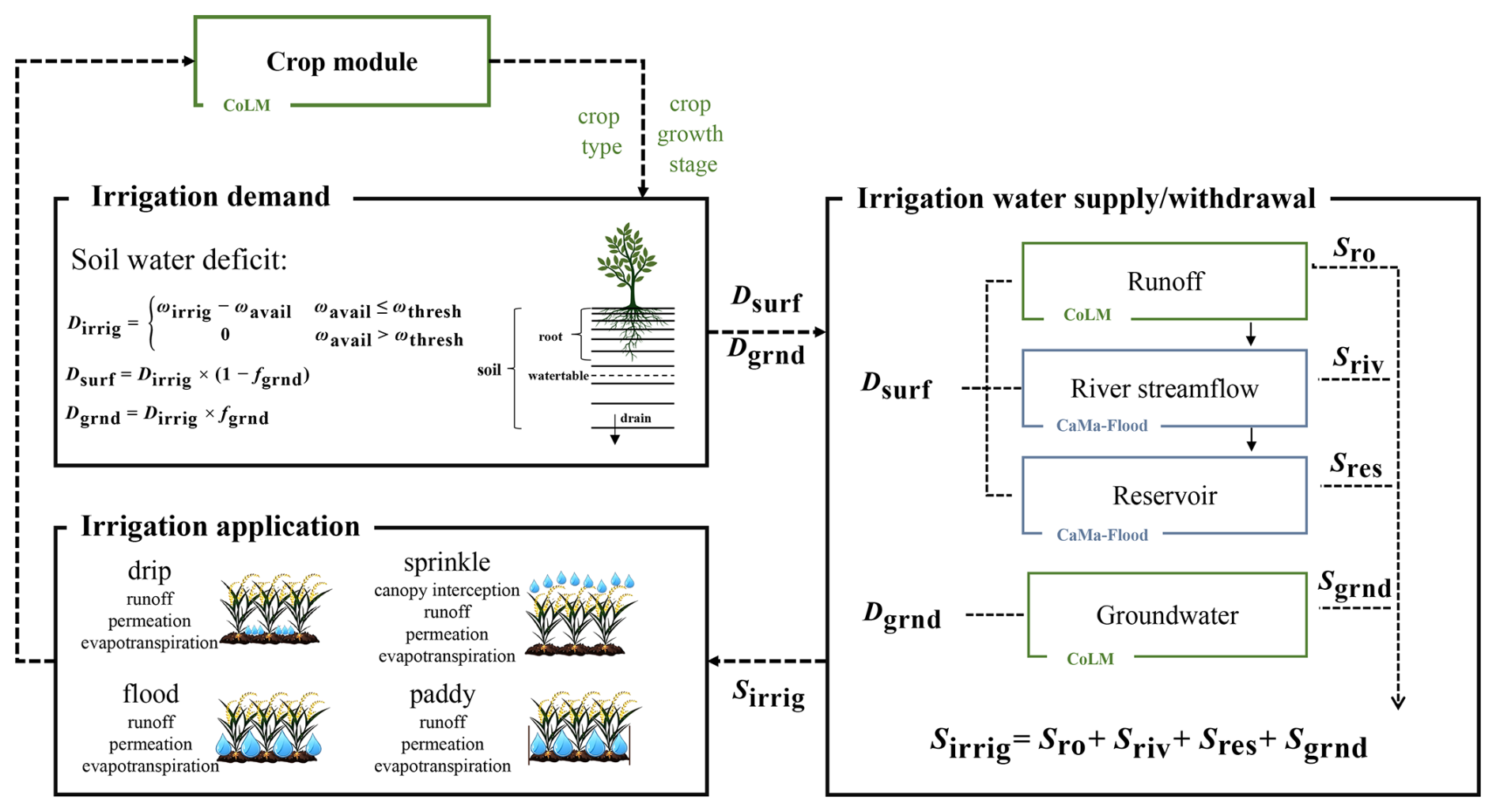
To enhance the representation of human–water interactions in land surface models, we introduce a new irrigation module for CoLM. This module provides a comprehensive framework for simulating the entire irrigation water system, including water demand, withdrawal, and utilization. It incorporates an irrigation water demand scheme based on soil moisture deficits, an irrigation application scheme accounting for four major irrigation methods, and an irrigation water withdrawal scheme that incorporates multiple water source constraints by integrating CoLM with a river routing model and a reservoir operation scheme. A key focus of this module is the bidirectional coupling between irrigation water demand and supply, alongside a detailed representation of water withdrawals from different sources. Section 2 provides a detailed description of the module and its implementation, including an overview of CoLM, the datasets used for simulation and validation, and the experimental design. Section 3 validates the module's performance in simulating irrigation water withdrawals using reported data and compares its results to other hydrological models. It also assesses improvements in model accuracy for regional energy dynamics (sensible heat, latent heat, and surface temperature), hydrology (river flow), and agricultural outputs (maize, soybean, and wheat yields). Section 4 demonstrates two key applications of the module: analyzing irrigation impacts on the energy budget and evaluating irrigation water security. Finally, we discuss the module's current limitations and propose potential future improvements.

2 Materials and methods

2.1 Description of CoLM and its crop module

The Common Land Model (CoLM) is one of the most advanced land surface models widely used to simulate the water–energy–carbon nexus. The original version of CoLM (Dai et al., 2003) combines the three land surface models: the Land Surface Model (LSM) of Bonan (1996), the Biosphere-Atmosphere Transfer Scheme (BATS; Dickinson et al., 1993), and the 1994 version of the Chinese Academy of Sciences Institute of Atmospheric Physics LSM (IAP94; Dai and Zeng, 1997). CoLM2014 integrates the Catchment-based Macro-scale Floodplain model (CaMa-Flood; Yamazaki et al., 2011), enabling river routing calculations within the model. Specifically, runoff generated by CoLM is transferred to CaMa-Flood for routing through the river network. CaMa-Flood represents the river network as a series of irregular unit catchments, defined through sub-grid topographic parameters. River discharge and other flow characteristics are computed using the local inertial equations along the river network, allowing for detailed flow dynamics across catchments.

In CoLM2024, the patch serves as the fundamental computational unit to account for land surface heterogeneity (Fig. S1). Based on land type, patches are divided into five types: vegetation (including bare soil), urban, wetlands, glaciers, and water bodies. The vegetation patch is further classified into natural vegetation and crops, represented using the plant functional type (PFT) approach. Under this framework, all natural vegetation within a grid cell is treated as a single patch, sharing common soil thermal and moisture conditions, while radiative and photosynthesis processes are simulated independently. When the crop model is activated, each crop type (distinguishing between rainfed and irrigated crops) is treated as an independent patch. This means that the calculations of soil moisture and thermal processes for each crop patch remain independent, without shared water and heat dynamics.

At each patch, the primary thermal processes include precipitation phase change; radiation transfer; temperature calculations for leaves, snow, and soil; and turbulent exchange, among others. The key hydrological processes include canopy interception, evapotranspiration, surface runoff, infiltration, soil water vertical movement, subsurface runoff, groundwater, and river routing, among others. Specifically, the two-big-leaf scheme is employed to compute radiation transfer, leaf temperature, photosynthesis, and transpiration (Dai et al., 2004; Yuan et al., 2017). Surface turbulent exchange is simulated using similarity theory (Liu et al., 2022; Zeng and Dickinson, 1998). Soil and snow temperature are determined using the heat diffusion equation, considering only vertical exchange (Dai and Yuan, 2014). Canopy interception is calculated the same as CoLM2014, considering the leaf angle and precipitation phase (Dai and Yuan, 2014; Sellers et al., 1996). Soil water vertical movement is simulated by the Richards equation and Buckingham–Darcy's law using the Campbell soil water characteristic curve scheme to close the Richards equation (Buckingham, 1907; Campbell, 1974; Richards, 1931). Surface and subsurface runoff are estimated using the SIMTOP approach (Niu et al., 2005). When the irrigation scheme is activated, irrigation water is applied to the canopy or top soil according to predefined irrigation methods and simulated irrigation amounts, thereby influencing the soil moisture and thermal processes within the irrigated patches.

The CoLM2024 version incorporates substantial updates over CoLM2014, particularly by introducing representations of biogeochemical cycles and human activity processes (e.g., crop growth and reservoir management). The new crop module introduces a phenological development scheme based on accumulated temperature, a biomass allocation scheme among different plant organs, and fertilization schemes (Drewniak et al., 2013). Crops are categorized into four organ pools: leaves, stems, fine roots, and grains. The growth stages are divided into three phases: sowing to emergence, emergence to grain filling, and grain filling to maturity, with carbon allocation ratios to roots, stems, leaves, and grains varying across these phases. Upon maturation, crops are harvested, with part of the carbon from the grains contributing to the yield, while a small portion (3 g) is reserved as seeds for the next growing season. For carbon assimilation, the module employs Farquhar's photosynthesis scheme (Collatz et al., 1992; Farquhar et al., 1980) and Ball–Berry's stomatal model (Ball et al., 1987; Collatz et al., 1991), treating maize as a C₄ crop and other crops as C₃. Additionally, the module accounts for the effects of heat stress, water stress, nitrogen stress, and ozone stress on yield (Li et al., 2024b; Lombardozzi et al., 2020). The module has been calibrated for various crops, including maize, soybean, spring and winter wheat, rice, cotton, and sugarcane, enabling accurate simulation of crop yields.

2.2 Two-way coupled irrigation water use module

2.2.1 Irrigation demand

The irrigation demand is calculated using the soil moisture deficit method (Leng et al., 2017; Ozdogan et al., 2010; Yao et al., 2022). During the crop growth stage, irrigation is triggered at 06:00 local time (LT) if the soil moisture in the root zone (z_irrig=1 m) falls below the threshold value (ω_thresh). The total irrigation water demand (D_irrig, mm) is then calculated using Eq. (1),

$$\begin{array}{}\text{(1)}& D_{\mathrm{irrig}}=\left\{\begin{array}{ll}{\mathit{\omega }}_{\mathrm{irrig}}-{\mathit{\omega }}_{\mathrm{avail}}& {\mathit{\omega }}_{\mathrm{avail}}\le {\mathit{\omega }}_{\mathrm{thresh}}\\ \mathrm{0}& {\mathit{\omega }}_{\mathrm{avail}}>{\mathit{\omega }}_{\mathrm{thresh}}\end{array},\right.\end{array}$$

where ω_avail is the total soil water amount in the root zone (mm), and ω_irrig is the irrigation target threshold (mm), calculated using Eq. (2),

$$\begin{array}{}\text{(2)}& {\mathit{\omega }}_{\mathrm{irrig}}=f_{\mathrm{irrig}}({\mathit{\omega }}_{\mathrm{target}}-{\mathit{\omega }}_{\mathrm{wilt}})+{\mathit{\omega }}_{\mathrm{wilt}},\end{array}$$

where ω_wilt is the wilting point soil water amount in the root zone (mm), calculated as the sum of soil water at the wilting point for each soil layer (${\sum }_{j=\mathrm{1}}^{N_{\mathrm{irr}}}{\mathit{\theta }}_{\mathrm{wilt}}\mathrm{\Delta }{z}_j$), and ω_target is the target soil water amount in the root zone (mm), calculated as the sum of target soil water for each soil layer (${\sum }_{j=\mathrm{1}}^{N_{\mathrm{irr}}}{\mathit{\theta }}_{\mathrm{target}}\mathrm{\Delta }{z}_j$). N_irr is the number of soil layers in the root zone, and Δz_j is the thickness of each soil layer (m). The target (θ_target) and wilting point (θ_wilt) soil moisture (m³ m⁻³) for each layer are calculated based on the corresponding soil water potential (Φ_target and Φ_wilt). f_irrig is a weighting coefficient ranging from 0 to 1, controlling the extent to which soil water amount approaches the target level ω_target during irrigation (default value = 1). In some cases, it can represent the efficiency of the irrigation system, accounting for water losses due to evaporation, seepage, or other factors.

The irrigation trigger threshold (ω_thresh) in Eq. (1) is calculated as

$$\begin{array}{}\text{(3)}& {\mathit{\omega }}_{\mathrm{thresh}}=f_{\mathrm{thresh}}({\mathit{\omega }}_{\mathrm{trigger}}-{\mathit{\omega }}_{\mathrm{wilt}})+{\mathit{\omega }}_{\mathrm{wilt}},\end{array}$$

where ω_trigger is the trigger water amount in the root zone (mm), and f_thresh is also a weighting coefficient ranging from 0 to 1 that controls the proximity of soil water amount to the trigger level ω_trigger (default value = 1). In this study, f_irrig and f_thresh were set to their default values.

The values of ω_trigger and ω_target are set according to the irrigation application method. For drip and sprinkler irrigation, both ω_trigger and ω_target are set to the soil field capacity water amount. For flood irrigation, ω_trigger is set to the soil field capacity water amount and ω_target to the saturation water amount. For paddy irrigation, both ω_trigger and ω_target are set to the saturation water amount.

2.2.2 Irrigation application

The model incorporates four different irrigation application methods: drip irrigation, sprinkler irrigation, flood irrigation, and paddy irrigation, each with unique triggering conditions, water demand requirements, and application processes. Drip irrigation is triggered when soil moisture in the root zone falls below field capacity, with the irrigation goal being to restore soil moisture to field capacity. This method applies water directly to the surface soil, allowing it to percolate into deeper soil layers. Sprinkler irrigation shares the same triggering condition and demand requirement as drip irrigation but applies water above the canopy. In this method, water can be intercepted and evaporated before reaching the soil surface, resulting in relatively lower irrigation efficiency. This method is the most commonly used in the United States. Flood irrigation is triggered when soil moisture falls below field capacity, to raise soil moisture to the point of saturation. Paddy irrigation is applied whenever soil moisture drops below saturation, aiming to restore soil moisture to saturation without causing runoff loss (Table S1). Paddy fields are typically maintained with a specific water level on the surface (10 cm) during the growing season. A global irrigation method map (Yao et al., 2022; Fig. S4) is used to determine the irrigation method for each grid. In addition, irrigation is implemented daily at 06:00 LT, if necessary, with water supply evenly distributed across each time step throughout the next 4 h.

2.2.3 Irrigation water supply/withdrawal

The model incorporates two distinct irrigation water supply/withdrawal schemes. The first scheme, unlimited supply (irrig-unlim), assumes that irrigation demand is fully met without accounting for specific water sources, a common approach in most land surface models (Yao et al., 2022). The second scheme, limited supply (irrig-lim), divides total irrigation demand between surface water and groundwater sources, labeled as surface water demand (D_surf) and groundwater demand (D_grnd), respectively. Both demands are constrained by the available water within each respective system. This distribution is based on the spatial extent of groundwater irrigation equipment, as provided by Siebert et al. (2010), and is formulated as follows:

$$\begin{array}{}\text{(4)}& {\displaystyle }{D}_{\mathrm{surf}}=D_{\mathrm{irrig}}\times (\mathrm{1}-f_{\mathrm{grnd}}),\text{(5)}& {\displaystyle }{D}_{\mathrm{grnd}}=D_{\mathrm{irrig}}\times f_{\mathrm{grnd}},\end{array}$$

where D_surf and D_grnd represent the demand from surface water and groundwater systems, and f_grnd denotes the area fraction covered by groundwater equipment. In this scheme, surface water demand (D_surf) is sourced sequentially from local grid cell runoff, local river streamflow, and upstream reservoirs, while groundwater demand (D_grnd) is drawn from groundwater aquifers.

Surface water supply

In our two-way coupled irrigation system (Fig. 1), the daily surface water supply for irrigation is constrained by surface water availability, which is simulated by CoLM (runoff) and CaMa-Flood (local streamflow and upstream reservoirs). We first examine whether the runoff from the local grid cell (S_ro) can meet the daily surface water demand (D_surf) for that cell. If runoff is insufficient, additional water is sourced from local streamflow and upstream reservoirs. River streamflow availability (S_riv) is determined by CaMa-Flood. For each irrigated grid cell, the river grid with the highest flow within a 250 km radius is selected as the source. To prevent excessive water extraction, a withdrawal limit is imposed, ensuring that the remaining flow in each river grid cell does not drop below 20 % of its average daily volume. Before conducting irrigation simulations, natural river flow simulations are performed to establish essential parameters for both river and reservoir water withdrawal schemes.

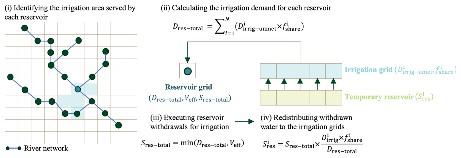
Reservoir water availability (S_res) is also determined by CaMa-Flood, which now includes a reservoir module. This module consists of the following components: (i) a reservoir dataset that provides reservoir location information matched with the river network, along with reservoir parameters (e.g., characteristic storage capacity); (ii) a reservoir operation scheme designed for flood control; and (iii) a routing scheme that integrates reservoir operations into river flow simulations. For more details, refer to Hanazaki et al. (2022). In this study, we further propose a new scheme for sourcing irrigation water from reservoirs (Fig. 2), which involves the following steps:

• i.

  Identifying the irrigation area served by each reservoir. It is challenging to accurately define the true irrigation extent/area for each reservoir, especially across large spatial domains. Therefore, a simplified approach is adopted here: larger reservoirs are assumed to cover a proportionately larger irrigation area, restricted to downstream regions only (since upstream water transfer is economically infeasible). Based on the relationship between reservoir size and the corresponding irrigation area provided in Table S2, we calculate the irrigation area for each reservoir according to its storage capacity by linear interpolation. Downstream irrigation grids are selected sequentially, from nearest to farthest, until the cumulative grid area closely matches the calculated irrigation area. If multiple reservoirs serve the same irrigation grid, a sharing proportion (f_share, ranging from 0 to 1) is assigned to the irrigation grid based on the degree of shared usage.

• ii.

  Calculating the irrigation demand for each reservoir by aggregating the demands of associated irrigation grids. This is expressed as $D_{\text{res-total}}={\sum }_{i=\mathrm{1}}^N\left(D_{\text{irrig-unmet}}^i\times f_{\mathrm{share}}^i\right)$, where $D_{\text{irrig-unmet}}^i$ and $f_{\mathrm{share}}^i$ represent the irrigation demand (i.e., the portion of D_surf not met by local runoff and river streamflow) and sharing proportion of grid i, respectively. N denotes the number of irrigation grids served by the reservoir.

• iii.

  Executing reservoir withdrawals for irrigation based on demands. Water is then withdrawn (S_res-total) from the reservoir's effective storage (V_eff) – the portion between the current water level and dead water level – according to the required demand. This is expressed as $S_{\text{res-total}}=min\left(D_{\text{res-total}},V_{\mathrm{eff}}\right)$. After updating the reservoir storage, the reservoir operation and subsequent river routing are calculated following the approach outlined in Hanazaki et al. (2022).

• iv.

  Redistributing withdrawn water to the irrigation grids. Based on each irrigation grid's contribution to the total reservoir irrigation demand, the total withdrawal volume is proportionally allocated across the associated grids ($S_{\mathrm{res}}^i$). This is expressed as $S_{\mathrm{res}}^i=S_{\text{res-total}}\times \frac{D_{\text{irrig-unmet}}^i\times f_{\mathrm{share}}^i}{D_{\text{res-total}}}$. Notably, this water is not applied directly to irrigation but is stored in a temporary reservoir (i.e., a temporary variable) for each irrigation grid in CoLM. This approach addresses the response delay in water supply from the river routing model to the land model's irrigation demands, as the time step for CoLM is 60 min, while CaMa-Flood operates with a 6 h time step and exchanges information with CoLM every 6 h. Moreover, if the reservoir cannot fully meet the irrigation demand within the initial time step, any unmet demand is carried forward to the next time step. This process continues over a 24 h cycle, after which new water demands for the next day are received.

Thus, the computational sequence proceeds as follows. Step (i) is completed before model execution, with its results serving as an essential input for the irrigation module. During model operation, CoLM calculates the irrigation demand at 06:00 LT. The unmet demand (after subtracting the water supplied by local runoff and streamflow) is then sent to CaMa-Flood, as described in step (ii). CaMa-Flood supplies water from the reservoir to meet this demand, as described in step (iii), and returns the supplied water to CoLM according to step (iv) over the next 24 h. During this process, the water supplied by the reservoir is stored in the temporary reservoir (variable) for each irrigation grid within CoLM. The following day, when irrigation begins again at 06:00 LT, water is withdrawn directly from the temporary reservoir if the demand cannot be met by local runoff and streamflow.

Figure 1 Diagram of the two-way coupled irrigation water system in the Common Land Model.

Figure 2 Diagram of the reservoir water supply scheme.

Groundwater supply

Groundwater supply is constrained by the availability of water within the aquifer. In CoLM, the groundwater table interacts with soil layers through vertical water exchange, allowing recharge or withdrawal of water from the aquifer (Li et al., 2017a). The evolution of the groundwater table is determined by the balance of soil water recharge and subsurface outflow, with the specific yield dynamically linking the water table position to changes in soil moisture and aquifer storage. When irrigation is required, water is directly extracted from the top of the simulated aquifer, and the water table depth is updated accordingly. This process continues until either the irrigation demand is fully met or the water table falls below a predefined threshold, set as 1 m below the initial depth at the beginning of the year (Jasechko et al., 2024; Russo and Lall, 2017). Groundwater supply is immediately available upon demand, with no temporal lag between the request and its availability for irrigation. Changes in the water table depth can then affect subsurface drainage and recharge from the bottom soil layer to the aquifer.

2.3 Materials

2.3.1 Input datasets

In this study, CoLM was implemented across the contiguous United States at a 0.25° spatial resolution for the period 2001–2016. Meteorological input data were derived from the WATCH Forcing Data methodology applied to ERA-Interim data (WFDEI) (Weedon et al., 2014a), which has also been utilized in the Inter-Sectoral Impact Model Intercomparison Project phase 2a (ISIMIP2a; Gosling et al., 2019). Soil property data were sourced from the Global Soil Dataset for Earth System Modeling (GSDE), originally provided at a spatial resolution of 30 arcsec (Dai et al., 2019; Shangguan et al., 2014a). Land cover data were derived from the MODIS dataset (MCD12Q1; Friedl and Sulla-Menashe, 2022), providing detailed global land classification information at a spatial resolution of 500 m.

The simulation of irrigation processes also required detailed data on crop areas, planting dates, irrigation areas, and irrigation methods. Crop planting areas were derived from the 30 m resolution CropScape and Cropland Data Layer (CDL) datasets (2008–2020) and aggregated to a spatial resolution of 5 arcmin for analysis (USDA/NASS, 2019). These datasets, produced by the U.S. Department of Agriculture, provide annual, crop-specific land cover information using satellite imagery and ground reference data. For each pixel, we calculated the proportion of cropland relative to the pixel's area (PCT_CROP) and the proportions of maize, wheat, and soybean relative to the cropland area (PCT_CFT). Pixels with a cropland percentage (PCT_CROP) exceeding zero were classified as crop pixels. The plant functional type (PFT) approach employed in CoLM allowed different crops and vegetation types to coexist within the same grid cell according to their percentages (PCT_CFT). To define planting and harvesting dates, we utilized an observation-based crop calendar dataset from the Global Gridded Crop Model Intercomparison (GGCMI), which provided information for 20 major crops under both rainfed and irrigated conditions at each grid cell for 1980–2010 (Jägermeyr et al., 2021a).

The irrigation map was derived using the 5 arcmin resolution data from the FAO Global Map of Irrigation Areas version 5 (Siebert et al., 2013). Since the CropScape data do not distinguish between rainfed and irrigated crops, we combined them with the irrigation map to determine the proportions of rainfed and irrigated crops. Irrigation water withdrawals were classified into surface water and groundwater sources following FAO data on regions equipped for groundwater extraction, which informed the allocation of irrigation demand across sources (Siebert et al., 2010). The irrigation application method data were obtained from Yao's global irrigation map, which details irrigation methods (drip, sprinkler, or flood) for 32 crop types, each assigned a single method (Yao et al., 2022). Jägermeyr et al. (2015) originally used a decision tree to refine AQUASTAT's data, classifying irrigation methods for 14 crop functional types (CFTs) based on crop area, soil characteristics, and socioeconomic conditions. Yao et al. (2022) then matched these CFTs to 32 crop types in CLM5 and incorporated an additional irrigation method, paddy, specifically for rice-growing regions, creating a more detailed global irrigation dataset.

For river routing simulations in CaMa-Flood, the baseline topography was derived from the Multi-Error-Removed Improved-Terrain Hydrography dataset (MERIT Hydro; Yamazaki et al., 2019). Fundamental information on dams/reservoirs in the river network, including dam name, coordinates, total storage capacity, and drainage area, was obtained from the GRanD database (Lehner et al., 2011a). GRanD version 1.3 contains data on 7320 dams globally, along with their associated reservoirs. The locations of the dams in the 0.25° river map were determined following the method outlined by Hanazaki et al. (2022), which enabled the identification of 1464 reservoirs across the contiguous United States (Fig. S3). In addition to GRanD, the Global Reservoir Surface Area Dataset (GRSAD; Zhao and Gao, 2018) and the Global Reservoir Geometry Database (ReGeom; Yigzaw et al., 2018a) were used to estimate reservoir parameters, such as storage capacity at emergency, flood control, and critical levels (Hanazaki et al., 2022). GRSAD provides a monthly time series of surface areas for 6817 GRanD reservoirs from 1984 to 2015, based on global surface water occurrence data (Pekel et al., 2016). ReGeom contains storage–area–depth information for 6824 reservoirs in GRanD, with geometry estimates derived from assumed surface and cross-sectional shapes, as well as data on reservoir extent, total storage, and surface area.

2.3.2 Validation datasets

To evaluate the scheme developed in this study, we focused on validating irrigation water withdrawal volumes, land fluxes (including energy fluxes and river flows) and crop yields in irrigated areas. We used hydrological survey data from the U.S. Geological Survey (USGS, 2023), which provided detailed statistics on total irrigation water withdrawals, categorized by surface and groundwater sources, every 5 years since 2000. Within the time frame of this study, data were available for the years 2005, 2010, and 2015. Building on this, Ruess et al. (2024) employed a global hydrological model (PCR-GLOBWB) to estimate annual, crop-specific irrigation water withdrawals from 2008 to 2020. Additionally, we compared the irrigation water withdrawal volumes simulated by our model with those generated by six other hydrological models – VIC, PCR-GLOBWB, MATSIRO, LPJmL, H08, and DBH – that participated in ISIMIP2a (Gosling et al., 2019). Although more hydrological models were included in ISIMIP2a, our comparison was limited to these six because they provided irrigation water withdrawal outputs. The simulations were driven by the WFDEI climate dataset, with a spatial resolution of 0.5° and covering the period from 1971 to 2010.

For land surface flux validation, we used monthly latent and sensible heat fluxes provided by FLUXCOM at a resolution of 0.5° (Jung et al., 2019). FLUXCOM leveraged FLUXNET site observations and extended these globally through machine learning algorithms, resulting in a global dataset for latent heat, sensible heat, and carbon fluxes. For temperature validation, we used land surface temperature data from 2001 to 2016 at a spatial resolution of 0.1° from the ERA5-Land reanalysis dataset (Muñoz-Sabater et al., 2021).

For streamflow validation, we utilized monthly streamflow data from the Global Runoff Data Centre (GRDC, 2023) for the period 2001–2016. To ensure robust validation, we excluded catchments with fewer than 5 years of data during the study period and focused on catchments significantly influenced by irrigation while minimizing the impacts of other anthropogenic activities. These selection criteria ultimately resulted in 77 catchments being included in the analysis (Fig. S10).

For terrestrial water storage (TWS) validation, we utilized monthly terrestrial water storage anomaly data from the Gravity Recovery and Climate Experiment (GRACE) mission for the period 2002–2016, with a spatial resolution of 0.5°, provided by the NASA Jet Propulsion Laboratory (Watkins et al., 2015; Wiese et al., 2016).

For crop yield validation, we relied on annual yield reports for irrigated and rainfed crops from the USDA NASS at the county level, which is regarded as a reliable source of yield statistics (USDA/NASS, 2023). The data for irrigated crops primarily covered the Central Plains of the United States, with limited coverage in the eastern and western regions. We aggregated our grid-based yield simulation results to the county level and performed validation only for regions and years with available USDA data.

2.4 Experimental design

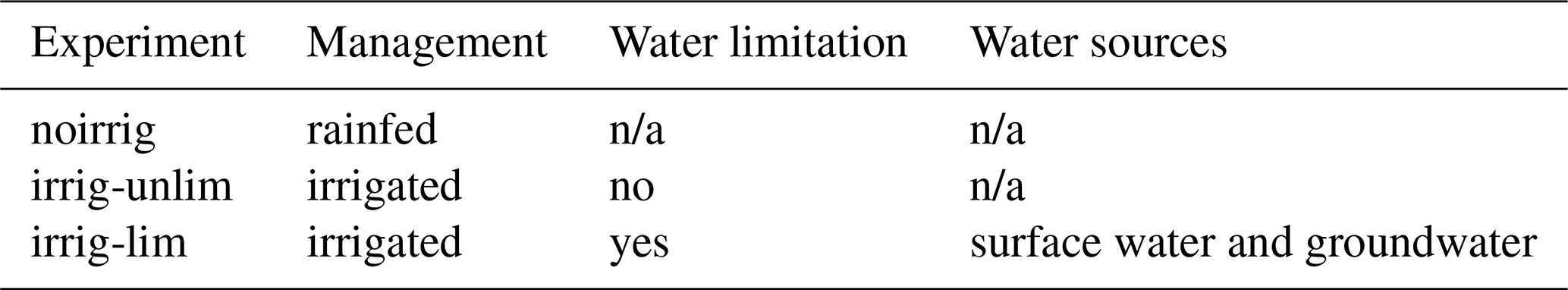
This study conducted three simulation experiments to evaluate the effectiveness of the newly developed module by comparing their performance:

• i.

  Non-irrigation experiment (abbreviated as noirrig). This scenario assumes all crops in the region are rainfed, with no irrigation applied. It serves as a baseline to represent natural surface water and energy balance conditions.

• ii.

  Unlimited irrigation experiment (abbreviated as noirrig-unlim). This scenario distinguishes between irrigated and rainfed areas based on crop maps. In irrigated areas, crop water demands are fully satisfied throughout the growing season, without considering the limitations of water resources.

• iii.

  Limited irrigation experiment (abbreviated as irrig-lim). In this scenario, irrigation water is supplied proportionally from surface water and groundwater based on availability, as illustrated in Fig. 1. Here, irrigation is constrained by the availability of surface and groundwater, which may result in unmet crop water demands.

The non-irrigation experiment was first simulated for the period 2001–2010 to stabilize vegetation carbon and nitrogen pools, soil moisture, and the groundwater table. This stabilized state served as the initial condition for all three experiments. The main simulation period spanned 2001–2016, covering the contiguous United States at a spatial resolution of 0.25° × 0.25°. In the subsequent analysis, key evaluation metrics – bias, root mean square error (RMSE), Pearson correlation coefficient (r), and Kling–Gupta efficiency (KGE) – were employed to assess the performance of the simulations.

Table 1 Experiment configurations. n/a: not applicable.

3 Results

3.1 Evaluation of simulated irrigation water withdrawal

3.1.1 Comparison with observations

Based on annual irrigation withdrawal data from the USGS, states in the western and central United States withdraw significantly more water for irrigation than those in the eastern regions (Fig. 3a). This is primarily due to the relatively low precipitation in the western and central regions, where the majority of irrigated areas are located, while crops in the eastern United States are predominantly rainfed. The top five states with the highest annual irrigation withdrawals – California (CA), Idaho (ID), Colorado (CO), Arkansas (AR), and Montana (MT) – are all situated in the Midwest and west (Fig. 3b). Nationally, the total annual irrigation withdrawal averages approximately 166.23 km³ yr⁻¹, based on data from 2005, 2010, and 2015. In comparison, the irrig-unlim and irrig-lim schemes simulate national total withdrawals of 290.94 and 120.81 km³ yr⁻¹, respectively. As illustrated in Fig. 3c–f, the simulations capture the spatial patterns of water withdrawals across different states effectively, with the irrig-lim scheme yielding better performance. The root mean square error (RMSE) and correlation coefficient (r) for the irrig-lim scheme are 3.60 km³ yr⁻¹ and 0.82, respectively, slightly outperforming the corresponding values for the irrig-unlim scheme (9.78 km³ yr⁻¹ and 0.76).

Irrigation water withdrawals draw from both surface water and groundwater sources. According to USGS reports, most irrigation withdrawals in the central United States come from groundwater (Dieter et al., 2018). In states such as Missouri (MO), Kansas (KS), Iowa (IA), Illinois (IL), Rhode Island (RI), and Mississippi (MS), the share of groundwater withdrawals exceeds 90 % (Fig. 4c). In contrast, states with high surface water withdrawals are primarily in the eastern and western United States, with states like Wyoming (WY), Connecticut (CT), Kentucky (KY), and Montana (MT) reporting surface water withdrawal proportions greater than 90 %. These spatial variations in water source usage are primarily attributed to the central United States's abundant groundwater resources and widespread groundwater extraction infrastructure.

In our simulations, the irrig-lim scheme effectively accounts for irrigation water withdrawals from different sources, constrained by their availability. Encouragingly, the scheme generally reproduces observed annual surface water and groundwater withdrawals across states (Fig. 4a–b), achieving correlation coefficients of 0.68 and 0.95, respectively. Furthermore, the simulated proportions of water sources closely align with observed data (Fig. 4c–d), with a correlation coefficient of 0.64 (p<0.01). However, the model tends to underestimate the surface water withdrawal proportions in the northwestern regions of the United States (particularly in Montana and Colorado; Fig. 4d), while slightly overestimating them in some central and eastern states. This discrepancy may stem from limitations in the data used to allocate water demand. Specifically, the model relies on predetermined groundwater extraction infrastructure proportions, which may not accurately reflect actual extraction practices, particularly as the dataset was published in 2005 and may not account for subsequent changes in groundwater infrastructure in certain states. Alternatively, the discrepancy could arise from model biases in simulating surface and groundwater availability. For example, in the northwestern region, surface runoff is heavily influenced by snowmelt and glacial meltwater (Li et al., 2017b), and biases in simulating these processes could lead to an underestimation of surface water availability.

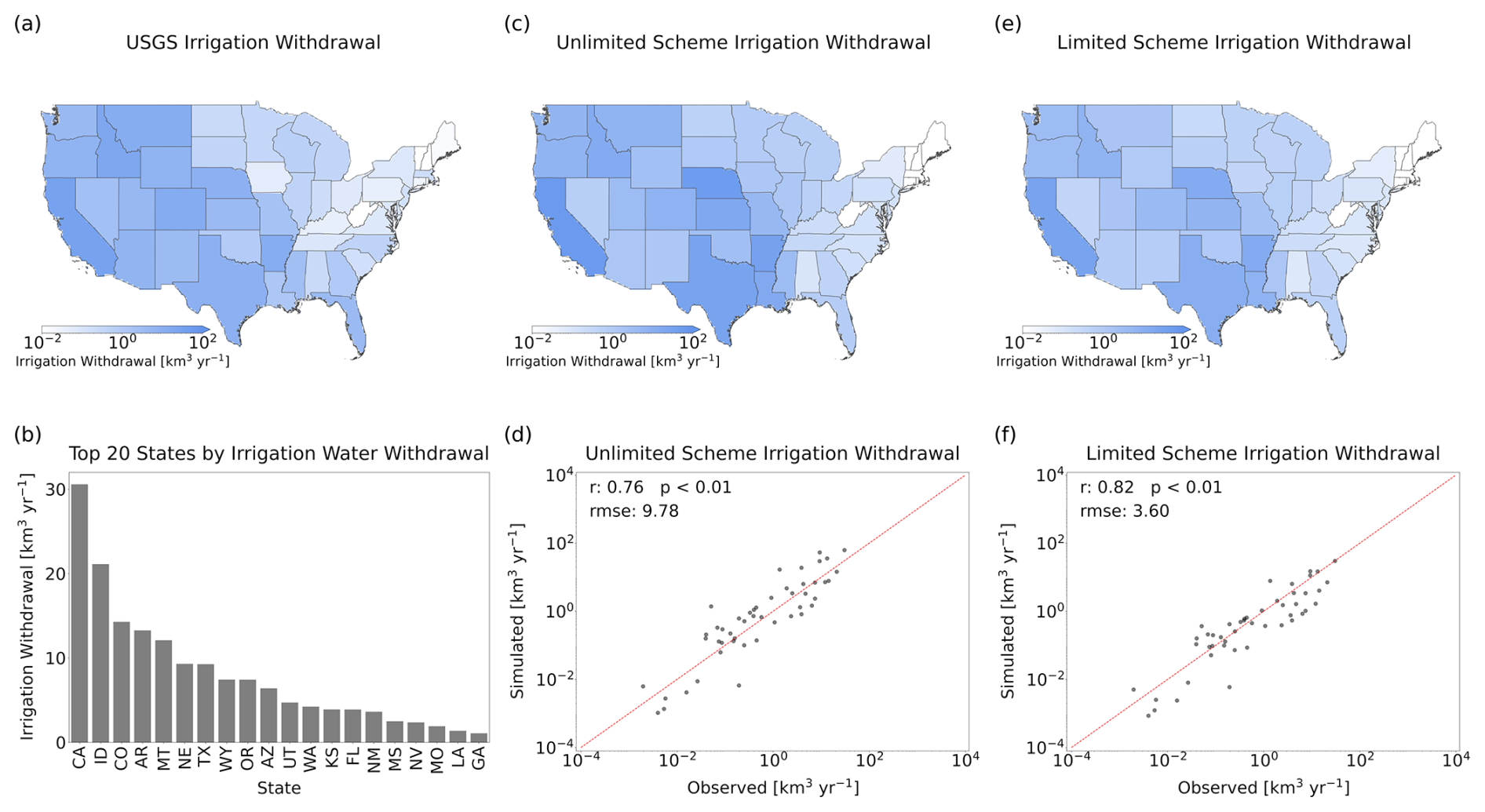
Figure 3 Comparison of reported and simulated irrigation water withdrawal in the United States. (a) Annual irrigation water withdrawal reported by the USGS for individual states. (b) Annual withdrawal amounts for the top 20 states by irrigation water withdrawal. (c) Annual irrigation water withdrawal simulated by CoLM using the unrestricted water supply (irrig-unlim) scheme for individual states. (d) Comparison of reported and simulated irrigation water withdrawal (using the irrig-unlim scheme) for individual states, with Pearson correlation coefficient (r) and root mean square error (RMSE) displayed, along with statistical significance (two-tailed Student's t test). (e) Annual irrigation water withdrawal simulated by CoLM using the restricted water supply (irrig-lim) scheme for individual states. (f) Comparison of reported and simulated irrigation water withdrawal (using the irrig-lim scheme) for individual states.

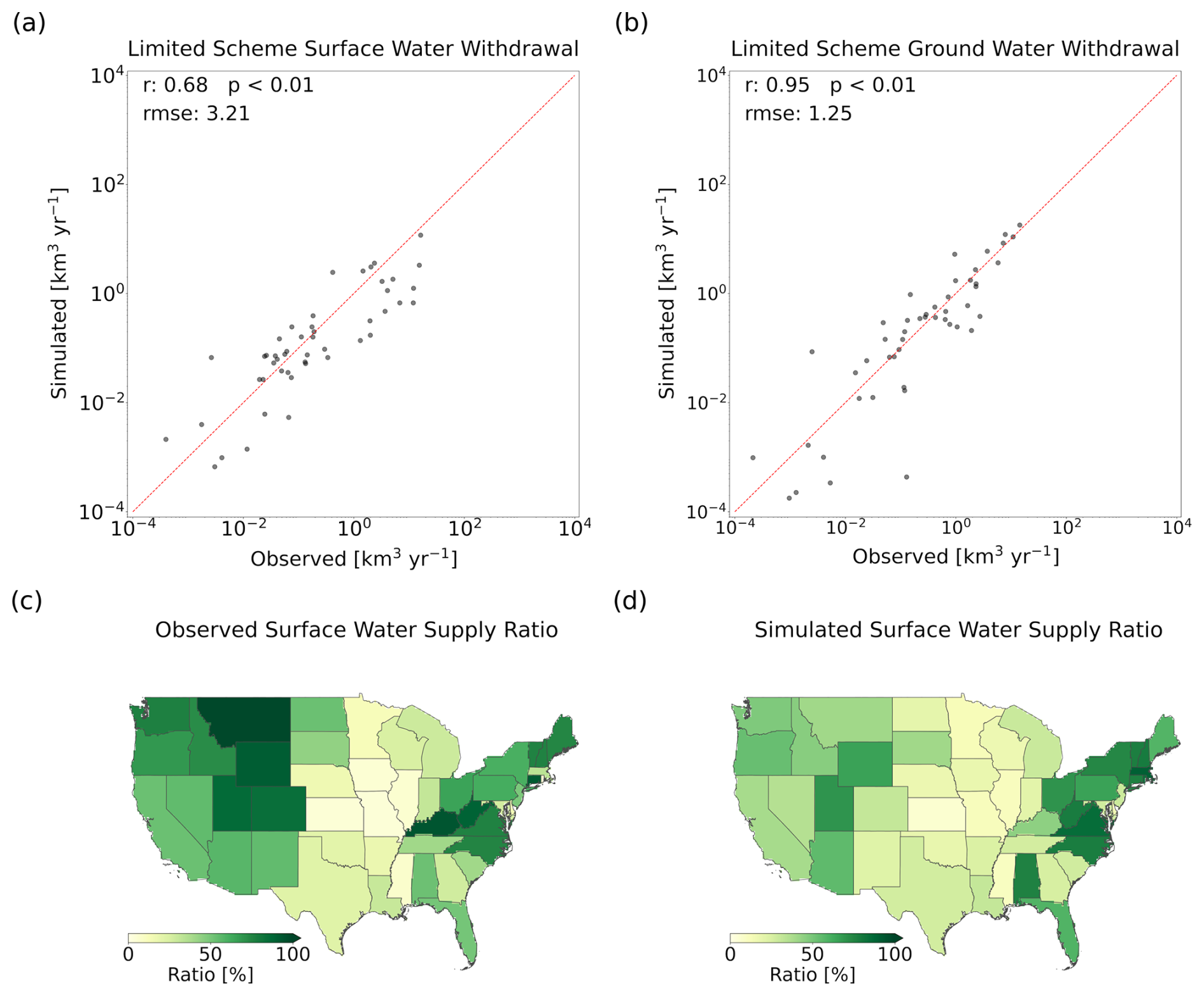
Figure 4 Comparison of reported and simulated irrigation water withdrawal in the United States by water source. (a) Comparison of reported and simulated surface water withdrawal volumes for individual states. (b) Same as panel (a) but for groundwater withdrawal volumes. (c) Proportion of surface water in irrigation withdrawal, based on USGS reports for individual states. (d) Proportion of surface water in irrigation withdrawal, simulated by CoLM using the irrig-lim scheme for individual states.

Ruess et al. (2024), using data from the USGS and model outputs from PCR-GLOBWB 2, generated an irrigation water withdrawal dataset that included withdrawal volumes for major crops in the United States. According to this dataset (Fig. 5), wheat is the largest consumer of irrigation water, with an average annual withdrawal of approximately 27.29 km³ yr⁻¹, followed by maize at about 20.91 km³ yr⁻¹. In contrast, soybean requires considerably less irrigation (i.e., 5.89 km³ yr⁻¹), partly due to its greater drought tolerance and smaller planted area compared to the other two crops. Under the irrig-unlim (irrig-lim) simulation scheme, the annual irrigation withdrawals for maize, wheat, and soybean are 53.98, 47.53, and 29.99 km³ yr⁻¹ (19.19, 17.95, and 11.05 km³ yr⁻¹), respectively. Once again, the irrig-lim scheme provides a closer alignment with observation-based data, as indicated by a lower RMSE (Fig. 5). These results suggest that our irrigation module generally performs well in simulating total national annual water withdrawals, the spatial distribution of withdrawals (Fig. 3), the proportion of water source types (Fig. 4), and the irrigation volumes for different crops (Fig. 5).

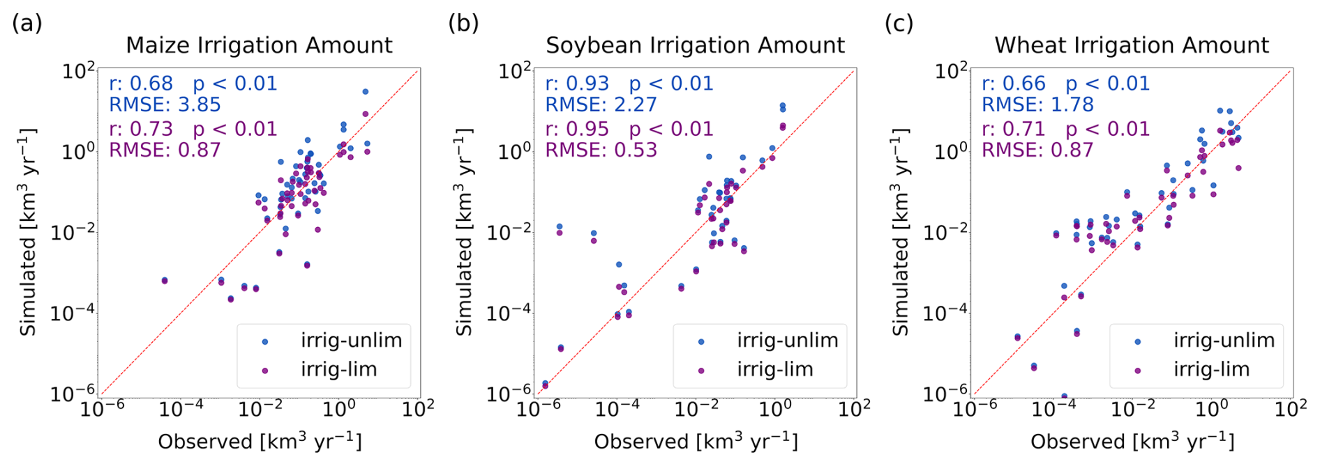
Figure 5 Comparison of reported and simulated irrigation water withdrawal in the United States by crop type. (a) Comparison of reported and simulated irrigation water withdrawal for maize, using both the unrestricted (irrig-unlim, blue dots) and restricted (irrig-lim, purple dots) supply schemes for individual states. (b–c) Same as panel (a) but for soybean and wheat.

3.1.2 Comparison with other models

We further compare the irrigation water withdrawal simulations from this study with outcomes from six global hydrological models (VIC, PCR-GLOBWB, MATSIRO, LPJmL, H08, and DBH) that participated in ISIMIP2a. Notably, all simulations used the same climate forcing (WFDEI), ensuring consistency in the comparison. Our results, particularly from the irrig-lim scheme, closely align with observed total national annual irrigation withdrawals. By contrast, five of the six models, excluding LPJmL, exhibit larger absolute deviations from observed value (Fig. 6a). Regarding spatial distribution, most models perform well (Fig. 6b), with LPJmL (orange dots) achieving the highest correlation coefficient (0.89) and the lowest RMSE (2.86 km³ yr⁻¹). The irrig-lim scheme in this study (purple dots) performs comparably to LPJmL, demonstrating competitive accuracy. In terms of temporal dynamics, comparisons across models are limited due to the scarcity of observed data. However, the general seasonal patterns are consistent across models (Fig. S6), with the highest irrigation withdrawals occurring in June and July and the lowest in January and December. Most models exhibit similar seasonal fluctuations, with irrigation volumes during peak months approximately 10 times greater than during off-peak months. Overall, these results suggest that our model performs similarly to, or even better than, existing models in simulating irrigation water withdrawals in the United States.

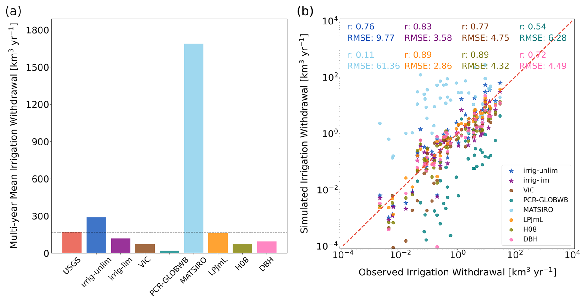
Figure 6 Comparison of irrigation water withdrawal simulated by CoLM and six global hydrological models participating in ISIMIP2a. (a) Annual total irrigation water withdrawal amounts in the United States as reported by the USGS, compared with simulations from CoLM (using both the irrig-unlim and irrig-lim schemes) and the six global hydrological models. (b) Comparison of reported and simulated irrigation water withdrawal for individual states, with Pearson correlation coefficient (r) and root mean square error (RMSE) for each simulation displayed.

3.2 Evaluation of simulated land energy and water fluxes

3.2.1 Evaluation of simulated energy fluxes

We evaluate CoLM's performance in simulating surface energy fluxes over irrigated areas in the United States using different schemes, with FLUXCOM monthly sensible heat (SH) and latent heat (LH) fluxes as observational references. Figure 7 compares multi-year monthly averages of observed and simulated SH and LH fluxes across irrigated grid points. Without irrigation (the noirrig scheme), the model significantly overestimates SH (Fig. 7a), with an average bias of 16.89 W m⁻² (44.53 %), and underestimates LH (Fig. 7c), with an average bias of 18.84 W m⁻² (37.11 %). In contrast, biases over non-irrigated grids are considerably lower, at 3.04 % and 17.38 % for SH and LH, respectively (Fig. S7). This indicates that CoLM performs satisfactorily in simulating energy processes over natural vegetation and rainfed areas but less so over irrigated regions.

With the inclusion of the irrigation module, simulation errors in surface energy fluxes over irrigated areas are significantly reduced, particularly in the US High Plains and the California Central Valley (Figs. S8 and S9). Under the irrig-unlim and irrig-lim schemes, average SH biases decrease to 27.10 % and 30.79 %, respectively, while LH biases decrease to 18.41 % and 22.18 %. These improvements are evident across most irrigated grid points, as illustrated by the kernel density estimate (KDE) curves of KGE, which indicate an increase in grid points with higher KGE values (Fig. 7). A KS test confirms that the differences between the irrigation (i.e., the irrig-unlim and irrig-lim schemes) and noirrig simulations are statistically significant. Although the irrig-unlim scheme performs slightly better than irrig-lim for SH and LH, this difference is not significant.

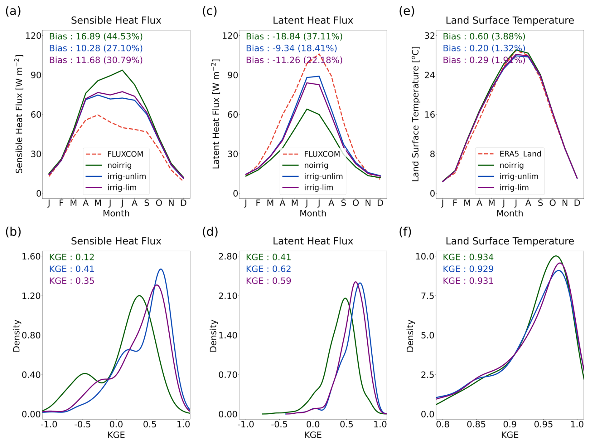
Figure 7 Evaluation of simulated energy fluxes and land surface temperature in the irrigation region. (a) Monthly sensible heat flux averaged from 2001 to 2016, based on FLUXCOM dataset and simulated by CoLM using the noirrig, irrig-unlim, and irrig-lim schemes in irrigation regions of the United States, with the bias between simulations and observations (i.e., FLUXCOM) indicated in the panel. (b) Kernel density estimate (KDE) curves for the Kling–Gupta efficiency (KGE) between observed and simulated monthly sensible heat flux for each irrigation grid, with mean KGE value indicated in the panel. (c–d) Same as panels (a)–(b) but for latent heat flux. (e–f) Same as panels (a)–(b) but for land surface temperature, using data from the ERA5-Land reanalysis dataset.

Additionally, the FLUXCOM data (dashed red line) show that the highest monthly SH and LH occur in May and July, respectively. However, the noirrig simulation (solid green line) fails to capture this seasonal peak, showing instead that SH peaks in July and LH in June. This discrepancy is not present in non-irrigated areas (Fig. S7), suggesting that irrigation in agricultural regions (and the subsequent crop growth it supports) substantially affects the seasonal pattern of regional energy balance. When the irrigation module is incorporated into the model, these seasonal patterns are more accurately reproduced, with the timing of the simulated peak months aligning more closely with FLUXCOM data (solid blue and purple lines).

The incorporation of the irrigation module improves the simulation of energy partitioning in irrigated areas, enabling the model to better capture surface temperature dynamics (Fig. 7e). Under the noirrig scheme, the average bias of monthly surface temperature is 0.6° (3.88 %). This bias decreases to 0.20° (1.32 %) with the irrig-unlim scheme and 0.29° (1.91 %) with the irrig-lim scheme. However, even with irrigation included, the simulated total evapotranspiration remains systematically underestimated (Fig. 7c). This underestimation is also evident in non-crop areas (Fig. S7c), suggesting that it may not be due to limitations in the irrigation module itself but rather to certain deficiencies in CoLM's evapotranspiration simulation approach.

3.2.2 Evaluation of simulated river flow

Irrigation processes can significantly alter natural hydrological dynamics and river flow patterns both temporally and spatially. To evaluate the effectiveness of the irrigation module in capturing these impacts, we compare model outputs with observed catchment streamflow data. We select catchments that are substantially influenced by irrigation while minimizing the effects of other anthropogenic activities. Figure S10 illustrates the locations of the selected 77 catchments. Figure 8 shows that CoLM's performance in simulating runoff – and consequently streamflow – remains limited, with relatively low average KGE values across all three schemes. This limitation is likely due to the use of a simplified runoff parameterization scheme in CoLM (Li et al., 2011). However, it is encouraging to note that the irrig-lim scheme notably improves monthly streamflow simulations compared to the noirrig scheme, increasing the average KGE from −0.57 to −0.49 and reducing the average percentage bias (PBIAS) from 117.28 % to 106.54 %. The enhancement can be largely attributed to the incorporation of irrigation effects, which account for reduced streamflow due to increased water use for evapotranspiration. This adjustment effectively mitigates the overestimation of streamflow observed in the noirrig scheme.

Our analysis reveals that the irrig-unlim scheme significantly reduces the accuracy of streamflow simulations compared to the noirrig scheme, leading to a pronounced overestimation of river discharge. This issue arises because the irrig-unlim scheme meets any irrigation demand by introducing additional water directly into the system without considering its source. Such an approach is common among crop and land surface models that incorporate irrigation (Malek et al., 2017; Yao et al., 2022; Zhang et al., 2020b). However, our findings indicate that introducing extra water for irrigation without accounting for its specific sources and limitations may lead to an imbalance in the water budget from a comprehensive perspective of the entire water system, undermining the model's ability to accurately represent the dynamics of the hydrological system. Furthermore, we compared observed and simulated monthly streamflow in 10 larger catchments (Fig. S12), providing a more intuitive assessment. The results clearly indicate that the irrig-lim scheme produces streamflow estimates that align more closely with observations, whereas the irrig-unlim scheme tends to overestimate streamflow, particularly during months with high irrigation demand.

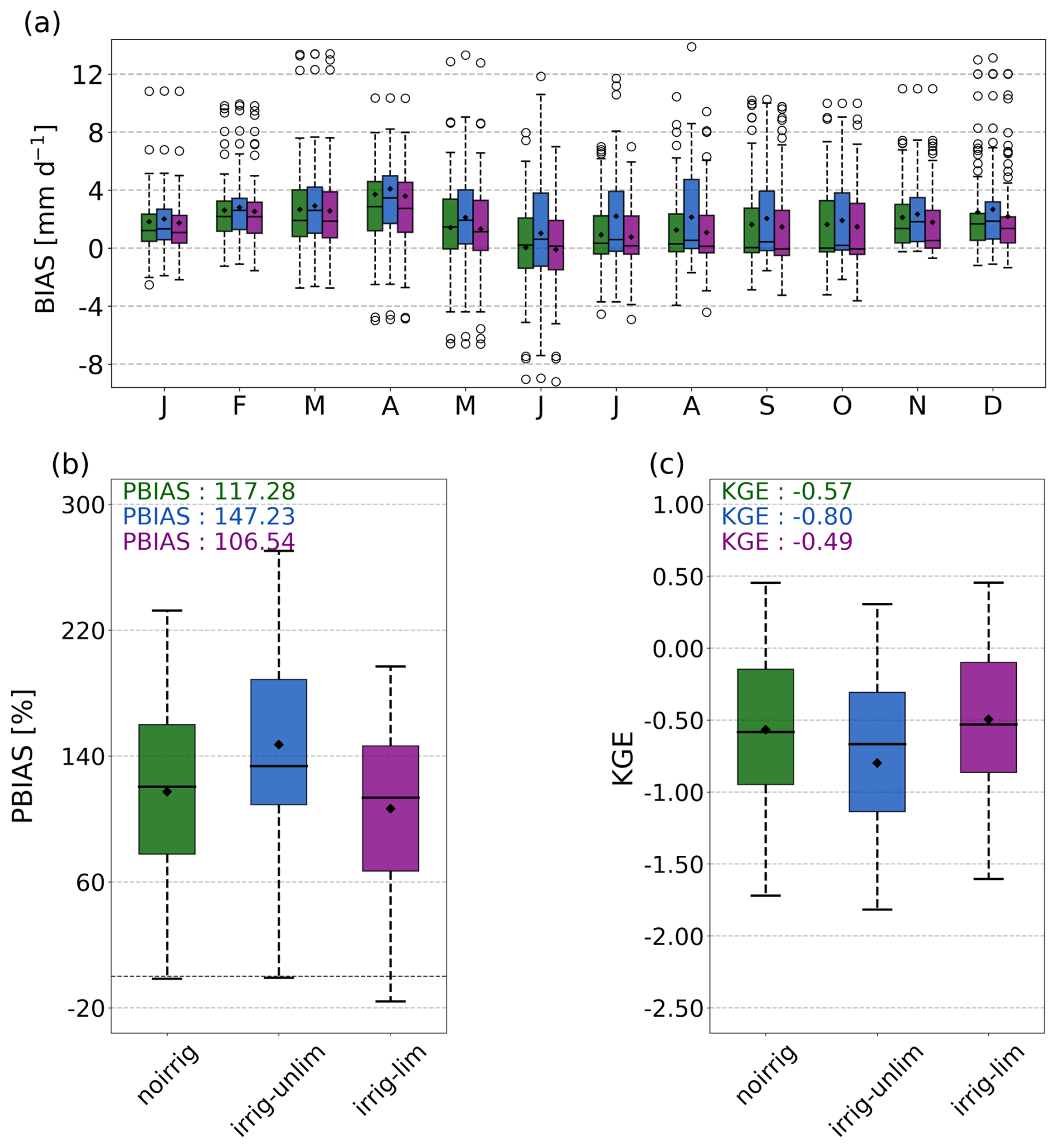
Figure 8 Evaluation of simulated streamflow in 77 irrigation-affected catchments. (a) Multi-year average monthly streamflow bias simulated using the noirrig, irrig-unlim, and irrig-lim schemes in the evaluation catchments. The boxes represent the interquartile range, black lines indicate median values, black dots show mean values, and dashed black whiskers extend to 1.5 times the interquartile range; points outside the boxes represent outliers. (b) Percentage bias (PBIAS) between observed monthly streamflow and simulations from CoLM under the noirrig, irrig-unlim, and irrig-lim schemes, with the average PBIAS value indicated in the panel. (c) Same as panel (b) but for the Kling–Gupta efficiency (KGE) between simulated and observed streamflow.

3.2.3 Evaluation of simulated terrestrial water storage anomalies

To assess the model's ability to simulate the impact of irrigation on terrestrial water storage (TWS) dynamics, we compared the simulated monthly TWS anomalies with those derived from GRACE satellite products provided by the NASA Jet Propulsion Laboratory. The results showed that incorporating the irrigation module, particularly under the irrig-lim scheme, improved the model's ability to capture both the interannual variability (Fig. 9a) and seasonal patterns (Fig. 9b) of TWS anomalies. Under the noirrig scheme, the simulated monthly TWS anomalies from 2002 to 2016 had a Pearson correlation of 0.25 with GRACE data and an RMSE of 6.75. In contrast, the irrig-lim scheme increased the correlation to 0.75 and reduced the RMSE to 5.13 (Fig. 9a). The spatial distribution of Pearson correlation coefficients between the simulations and GRACE data (Fig. S13) further demonstrated a widespread improvement across the United States, particularly in the Corn Belt.

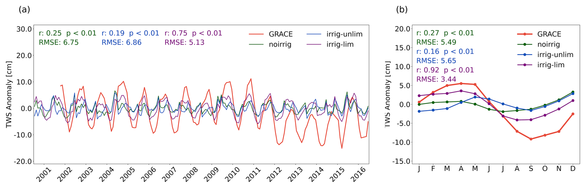
Figure 9 Evaluation of simulated terrestrial water storage anomalies in irrigated regions. (a) Time series of monthly terrestrial water storage anomalies from 2001 to 2016, simulated by CoLM (under the noirrig, irrig-unlim, and irrig-lim schemes) and derived from GRACE (JPL dataset). The Pearson correlation coefficient (r) and root mean square error (RMSE) between the simulations and GRACE data are indicated in the panel. (b) Climatological monthly terrestrial water storage anomalies averaged over 2001–2016, simulated by CoLM and derived from GRACE.

The enhancement was even more pronounced in the simulation of seasonal TWS anomaly patterns. Without irrigation, the model underestimated seasonal variations, resulting in a pattern that deviated substantially from GRACE observations. This bias was effectively corrected in the irrig-lim scheme, where the Pearson correlation coefficient increased to 0.92 and the RMSE decreased to 3.44 (Fig. 9b). However, none of the simulations captured the decline in GRACE-derived TWS anomalies during 2012 to 2016, likely due to groundwater depletion from irrigation (Rodell and Reager, 2023). This suggests that the model may require further validation and improvements in simulating irrigation-induced groundwater storage changes.

3.3 Evaluation of simulated crop yield

Irrigation reflects a direct human influence on crop yields by providing supplemental water. Crop models primarily focus on this aspect, but they often neglect how irrigation affects other processes. Conversely, most hydrological models concentrate on the impact of irrigation withdrawals on the water cycle, with some also addressing energy fluxes, yet pay less attention to crop yield. From this perspective, land surface models offer distinct advantages; they provide a more detailed representation of hydrological and surface energy processes compared to crop models, while also presenting more physics-based representations of crop growth than traditional hydrological models. Therefore, this study further evaluates whether incorporating the developed irrigation module can enhance crop yield in the simulations.

Using county-scale crop yield data for irrigated and rainfed regions provided by the USDA, we assess simulated yields under both irrigated and non-irrigated scenarios. The dataset may not comprehensively cover all irrigated areas in the United States or all years during the study period, so comparisons are limited to regions and years with reported data. In rainfed regions, the model broadly reproduces average annual yields for the maize, soybean, and wheat (Fig. S14). However, in irrigated regions, the model without irrigation significantly underestimates crop yields, with average underestimations of 31.95 %, 44.45 %, and 35.95 % for maize, soybean, and wheat, respectively (Fig. 10). Under both the irrig-umlim and irrig-lim schemes, despite slight differences in performance across crops, the model effectively simulates yield increases under irrigation, aligning well with observations. As shown in Fig. S15, the yield underestimation observed in most counties without irrigation is substantially corrected under the irrig-unlim (and irrig-lim) schemes, with 90.5 % (70.8 %), 99.5 % (94.2 %), and 68.4 % (74.8 %) of counties showing absolute yield differences for maize, soybean, and wheat within 1 t ha⁻¹ compared to observations. Differences between the two irrigation schemes are minimal: the irrig-unlim scheme performs slightly better for maize and soybean in terms of average biases, while the irrig-lim scheme shows better performance for wheat.

Furthermore, based on limited annual yield data, we observe that considering irrigation generally improves the model's ability to capture inter-annual yield fluctuations (Fig. S16). The KGE values of annual yields under the noirrig scheme are −1.342, −1.451, and −1.308 for maize, soybean, and wheat, respectively, while with the irrig-umlim and irrig-lim schemes the KGE values increase to 0.101, −1.132, and 0.197 and to −0.158, −1.449, and −0.144, respectively.

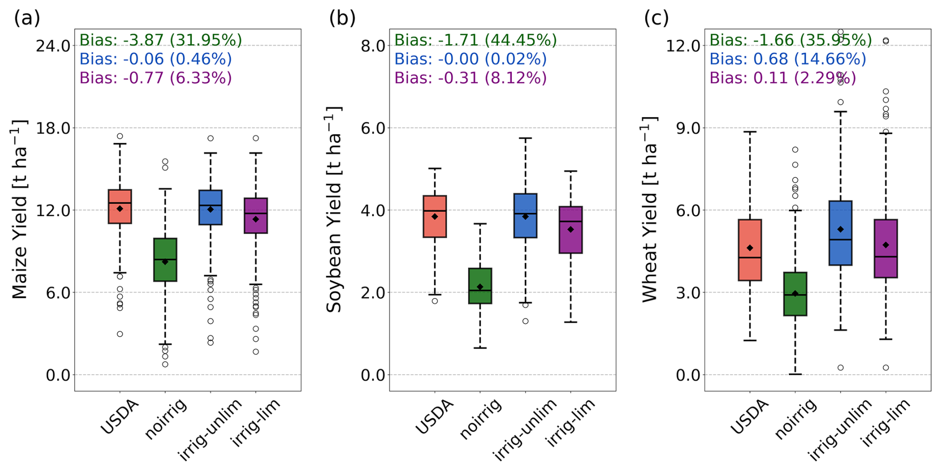
Figure 10 Evaluation of crop yield simulated using different schemes in the United States. (a) Maize yield in irrigated maize-growing regions of the United States, as reported by the USDA (orange boxes), compared with simulations by CoLM using the noirrig (green boxes), irrig-unlim (blue boxes), and irrig-lim (purple boxes) schemes. Since reported yields are at the county scale, grid-based simulation results were aggregated to corresponding counties. (b–c) Same as panel (a) but for soybean and wheat yields.

4 Discussions

4.1 Applications of the developed module

4.1.1 Impacts of irrigation on energy budget

Numerous studies have highlighted the impacts of irrigation on global and regional energy budgets and near-surface climates. In this study, we similarly examine the effects of irrigation on the energy budget over irrigated areas in the United States by comparing results from the irrig-lim and noirrig scheme. Consistent with prior research, we find that irrigation increases latent heat (LH) by 7.53 W m⁻² (23.25 %) and decreases sensible heat (SH) by 5.18 W m⁻² (9.48 %) averaged from 2001 to 2016, resulting in an approximately 0.30 °C reduction in land surface temperature (Fig. 11). Since land–atmosphere coupling is not included, the primary mechanisms driving these impacts are increased soil evaporation due to enhanced soil moisture and greater vegetation transpiration driven by improved crop growth following irrigation (Fig. S17a–b). Annually, these mechanisms contribute roughly equally to the increase in total evapotranspiration in irrigated regions, with pronounced seasonal differences: during the peak growing seasons (summer and autumn), the contribution was dominated by vegetation transpiration, while in other seasons, particularly winter, the increase in soil evaporation plays a larger role in affecting regional energy distribution and temperature (Fig. S17c).

This study further explores the spatial characteristics of these impacts, analyzing the correlations between irrigated area; irrigation water withdrawal; and changes in LH, SH, and land surface temperature (ΔLH, ΔSH, ΔT_s) across different climate zones. Notably, irrigation has the most substantial impact in arid regions, especially on LH, where ΔLH is more than double that of semi-arid and humid regions, with a larger reduction in temperature by 0.36 °C. Interestingly, while previous studies have emphasized irrigated area as the primary determinant of irrigation-induced climate effects (Al-Yaari et al., 2022; Chen and Dirmeyer, 2019), our results indicate that irrigation water withdrawal has a stronger influence on the regional energy budget and temperature. Across all climate zones, ΔSH, ΔLH, and ΔT_s are significantly correlated (p<0.01) with irrigation water withdrawal, with correlation coefficients of −0.81, 0.79, and −0.82, respectively (Fig. 11b, e and h), which are higher than the correlations with irrigated area (−0.59, 0.61, and −0.52; Fig. 11c, f and i). This emphasizes the critical role of water availability in modulating the climate effects of irrigation.

It is important to note that this study employs offline land simulations, which do not capture land–atmosphere interactions, potentially introducing biases in the estimated climate impacts. Previous studies have demonstrated that irrigation can induce both cooling and warming effects. While increased evapotranspiration contributes to cooling, irrigation can also enhance atmospheric water vapor content, leading to greater absorption of longwave radiation and potential cloud formation, resulting in warming (Dessler and Sherwood, 2009; Hu et al., 2019). These processes cannot be adequately represented in offline simulations, likely leading to an overestimation of irrigation-induced cooling and a subsequent underestimation of temperature (Fig. 11g). Future studies should incorporate coupled land–atmosphere simulations to provide a more comprehensive assessment (Cook et al., 2015; Puma and Cook, 2010; Sacks et al., 2009). Another aspect worth considering is that some farmers irrigate not only to address water deficits but also to mitigate heat stress during high-temperature periods (Verma et al., 2020). This practice can notably affect local temperatures. For instance, surface water temperatures generally track air temperatures, whereas groundwater temperatures remain relatively stable throughout the year – typically warmer than air in winter and cooler in summer. This temperature difference, especially in regions relying on groundwater irrigation, may have non-negligible effects on local climate that should be incorporated into future modeling efforts.

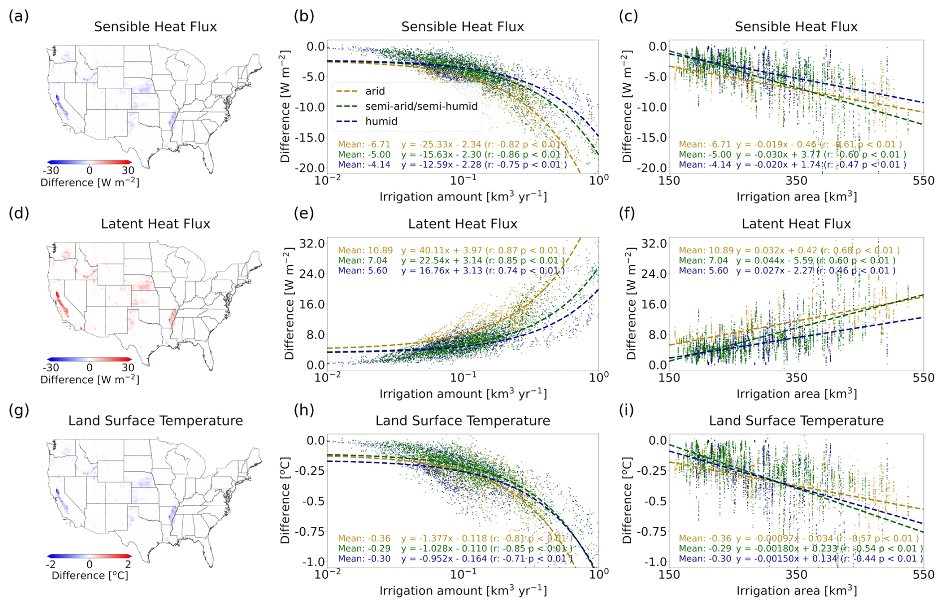
Figure 11 Impact of irrigation on local energy flux and surface temperature in the United States. (a) Impact of irrigation on sensible heat flux, quantified by the difference (ΔSH) between the noirrig and irrig-lim simulation results. (b) Relationship between irrigation amount and ΔSH, with grid colors indicating the climate zones (i.e., arid, semi-arid/semi-humid, humid). For each climate zone, the mean ΔSH, the regression line of irrigation amount versus ΔSH, and the regression equation are displayed. (c) Same as panel (b) but for the relationship between irrigation area and ΔSH. (d–f) Same as panels (a)–(c) but for the impact on latent heat flux (ΔLH). (g–i) Same as panels (a)–(c) but for the impact on land surface temperature (ΔT_s).

4.1.2 Assessments of irrigation water security

This study compares the irrigation schemes with and without water availability constraints, highlighting the necessity and importance of incorporating water limitations into simulations. Our results demonstrate that including these constraints improves simulation accuracy, particularly in the modeling of water systems. Specifically, irrigation water withdrawal simulated under the irrig-lim scheme aligns more closely with observational data (Figs. 3 and 6). Validation against river flow observations further supports the improved performance of the irrig-lim scheme. Importantly, this scheme avoids the risk of potential water imbalances in the modeled hydrological system – an issue commonly associated with non-constrained schemes (Fig. 8).

Additionally, incorporating water availability constraints more accurately reflects the reality of water resource utilization. By accounting for the interconnections between subsystems within the irrigation water demand–supply system, this approach enables simulation and prediction of irrigation water security issues. Here, we visualize the average number of days when water supply was insufficient to fully meet irrigation demand simulated by the irrig-lim scheme (Fig. 12). Spatially, in humid regions, where irrigation demand is low and water resources are abundant, fewer days of unmet irrigation needs occur. Conversely, in arid regions, where irrigation demand is high and water resources are often limited, the number of unmet irrigation days increases significantly. Figure 12a illustrates that states with a higher number of unmet irrigation days are also those with relatively scarce water resources (e.g., Montana and Nevada). From a temporal perspective, drought years lead to increased irrigation requirements due to reduced precipitation or higher evaporative demand. Although additional water withdrawals can partially address this increased demand, drought conditions often simultaneously result in deficits in both surface and groundwater resources within the water system. As a result, most states experience a substantial increase in unmet irrigation days during drought years (an average of 43 d). In contrast, during wetter years, the number of unmet days decreases significantly (an average of 31 d).

Reported disaster data show that even with irrigation, significant crop losses can occur during drought years, aligning with broader water security challenges (Mieno et al., 2024). Our approach effectively captures this phenomenon by describing the connectivity between subsystems in the water demand–supply system and highlighting the impact of water limitations on irrigation. In contrast, ignoring these constraints risks underestimating potential food security issues in a future characterized by more frequent and/or severe droughts. This represents a critical limitation of crop and land surface models that adopt irrigation schemes without considering water availability constraints.

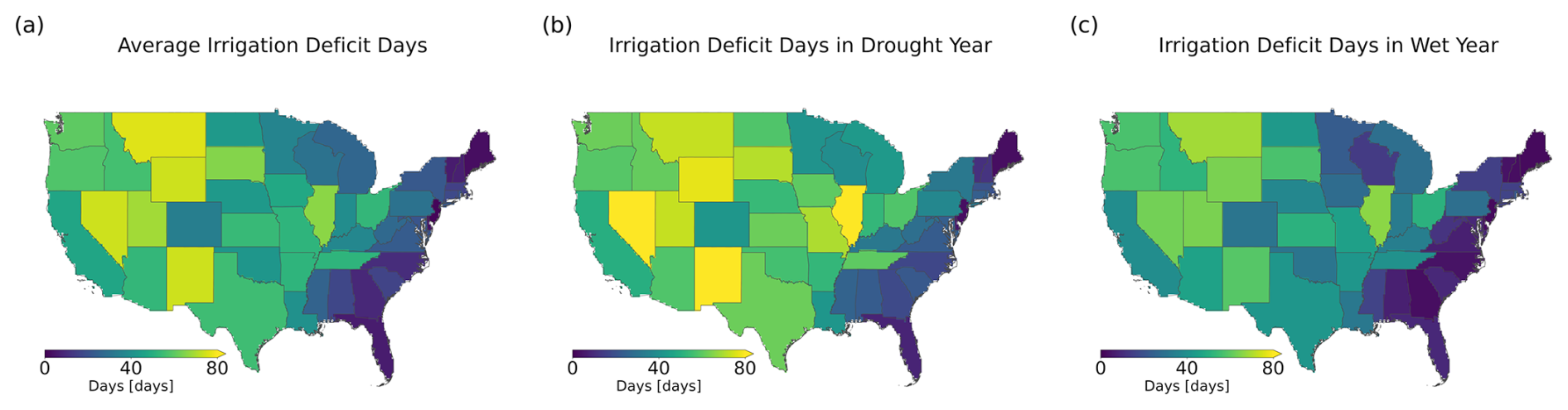
Figure 12 Days per year with unmet irrigation demand (i.e., irrigation deficit days) in the United States simulated by the irrig-lim scheme. (a) Multi-year average irrigation deficit days from 2001 to 2015 for individual states. (b) Irrigation deficit days in drought year for individual states. (c) Irrigation deficit days in wet year for individual states. Drought year (wet year) is defined as the year with the lowest (highest) annual precipitation during 2001–2016.

4.2 Limitations and a way forward

While the developed module represents a significant advancement in modeling the irrigation water system within land surface models by providing a comprehensive representation of the irrigation processes, including water demand, water withdrawal, and water utilization, several limitations and assumptions should be acknowledged.

Irrigation water demand in this study is estimated using a soil moisture deficit method. However, the parameterization of certain key variables (e.g., target and threshold soil moisture levels) is overly simplified and does not account for variations among crop types. These parameters are adjustable, and their calibration could further enhance the model's accuracy in reproducing irrigation water use. Similarly, the fixed root depth of 1 m for all crops introduces additional uncertainty, potentially leading to overestimation or underestimation of irrigation demand. Incorporating dynamic root growth could better represent actual root-zone depth based on crop-specific characteristics. Additionally, in some cases, farmers irrigate not only to address soil moisture deficits but also to reduce crop heat stress during high-temperature periods – a factor that should be incorporated into future modeling efforts. Furthermore, this study did not account for water losses during conveyance and application. Irrigation losses, as noted by Jägermeyr et al. (2015), include conveyance losses and on-field application losses. By ignoring conveyance losses, the model assumes that water withdrawn equals water applied, likely leading to an underestimation of total irrigation water use. Field application losses depend on irrigation methods (Leng et al., 2017), and while this study considered four irrigation systems with differentiated efficiencies, the reliance on simplified rules and a coarse irrigation map fails to reflect the diversity of irrigation methods and distributions. For example, actual sprinkler systems distribute water in specific spray patterns rather than uniformly. However, the model assumes uniform water distribution across each crop functional type (CFT). Future models could benefit from parameterizations that capture spatial heterogeneity in irrigation distribution (Jägermeyr et al., 2015; Merriam et al., 1999). Moreover, irrigation water demand also depends on agricultural practices, such as crop types, cropping calendars, and planting intensities. While the model determines crop phenology based on meteorological data, real cropping calendars are influenced by farmers' decisions (Sacks et al., 2010). Incorporating satellite-derived phenology data could better represent these human factors. Addressing these agricultural practices is crucial for improving the accuracy and applicability of irrigation models.

In simulations of irrigation water withdrawal, this study provides a detailed representation of reservoir water withdrawal but acknowledges several sources of uncertainty: first, the dataset includes fewer dams than exist, as it focuses primarily on large dams and may lack data due to protection policies. This omission likely contributes to the underestimation of surface water extraction in some states. Second, all dams are assumed to supply irrigation water, although some reservoirs may not serve this purpose. The irrigation areas served by each dam are unknown, and a generalized estimation method is employed in this study, introducing large uncertainties that remain difficult to validate. Third, dam operations are simplified, while in reality they often involve complex considerations, such as multi-objective operations and coordinated management of multiple reservoirs. Advanced reservoir optimization strategies, which require predictive simulations and prior knowledge of future inflows and demands, are not incorporated into the model, presenting a significant challenge for considering the impacts of complex human decision-making in land surface models.

Determining the division of irrigation water withdrawals between surface and groundwater sources, as well as the withdrawal sequence, is also critical. This study allocates irrigation demand based on predefined proportions and simultaneously withdraws water from both sources. Surface water demand is met sequentially through local runoff, river discharge, and upstream reservoir storages. This method, employed in models such as ORCHIDEE v2.2 (Arboleda-Obando et al., 2024) and E3SM (Zhou et al., 2020), provides satisfactory simulations of water source allocation for irrigation (Fig. 4 vs. Fig. S19). However, its reliability depends on the accuracy of input data and may underestimate withdrawals if any water source is inadequately represented. Alternatively, some models (e.g., MATSIRO and CLM5; Pokhrel et al., 2012; Yao et al., 2022) do not pre-allocate demand but set a fixed order of water withdrawals – typically prioritizing surface water before groundwater. This method tends to satisfy more irrigation demand and provides better estimates in regions with unreported groundwater extraction. We propose that a hybrid approach, defining surface and groundwater proportions dynamically, warrants consideration in future study. For instance, during wet seasons, surface water extraction proportions could increase to reduce groundwater reliance and associated pumping costs. Conversely, during dry seasons, surface water may be more constrained, necessitating greater reliance on groundwater for irrigation. However, such an approach still needs to address challenges, including unreported groundwater use; data scarcity; and the physical, technical, and socioeconomic constraints on groundwater use across regions.

Additionally, this study does not account for restrictions beyond water availability, such as local regulations governing water allocation, including water rights and inter-basin water transfers. Alternative water sources, such as desalinated seawater and treated wastewater, also warrant consideration (van Vliet et al., 2021). Recent assessments indicate that these unconventional water sources are experiencing exponential growth (Jones et al., 2019). Although their contributions remain low globally, they play a significant role in water-scarce regions. Incorporating these factors into models could further improve simulations of irrigation water security.

The developed module's results and applicability are also strongly influenced by the CoLM framework itself. A critical aspect requiring careful consideration is the evaluation and calibration of hydrological variables, such as soil moisture, runoff, river discharge, and groundwater levels, which are essential for water resource modeling. Currently, the CoLM employs the simplified TOPMODEL (SIMTOP) developed by Niu et al. (2005) for runoff simulations. The excessive simplification of this approach, coupled with the lack of calibration, limits the model's accuracy in runoff simulations. Inadequate representation of snow and glacial melt processes introduces regional biases, particularly in northern and midwestern US states where these factors are pivotal. For instance, surface water extraction is underestimated in some states within these regions, likely because the model fails to accurately capture snowmelt and glacial melt contributions to streamflow, leading to erroneous estimates of surface water availability. Similarly, simulated evapotranspiration is systematically underestimated, even in areas without crops or irrigation, likely due to more complex underlying causes. These biases, when aggregated at the watershed level, result in significant discrepancies in river discharge, thereby constraining the model's applicability for water resource management and its ability to predict irrigation water security. Addressing these issues requires urgent improvements in the representation of related processes, along with further calibration and parameter tuning.

Although the validation in this study is limited to the United States, the framework can be applied to other regions with appropriate datasets. For example, the module requires defining the allocation and sequence of withdrawals from surface water and groundwater sources. When applying the model to other regions, the groundwater and surface water withdrawal ratios should be predefined based on local infrastructure, such as groundwater extraction facilities, and the withdrawal sequence can also be adjusted accordingly. For surface water withdrawals, it is essential to prepare river network data and reservoir information for CaMa-Flood simulations. Additionally, improving simulation accuracy may require incorporating region-specific crop distribution (distinguishing rainfed and irrigated areas), crop characteristics (e.g., phenology, photosynthetic capacity, carbon allocation), and management practices (e.g., planting dates, irrigation strategies). Furthermore, CoLM offers multiple parameterization schemes for thermal, hydrological, and biogeochemical processes, which should be evaluated for their suitability in the target region.

5 Conclusions

The growing challenges posed by increasing global food demand and water scarcity underscore the need for advanced modeling tools capable of accurately capturing human–water interactions. This study contributes to addressing this need by implementing a two-way coupled irrigation water system within the Common Land Model. The developed module provides a comprehensive representation of the entire irrigation water use process, including water demand, withdrawal, and utilization. It introduces a refined multi-source water withdrawal framework and achieves bidirectional coupling between water demand and withdrawal during simulation.

The robustness of the new irrigation module is validated through simulations across the contiguous United States, focusing on regional-scale water, energy, and crop yield dynamics. The module effectively simulates total national annual irrigation withdrawals, their spatial distribution, the proportions of different water sources, and irrigation volumes for various crops. Compared to other hydrological models in ISIMIP2a, our model performs similarly or better in simulating US irrigation withdrawals. Incorporating the new irrigation module also significantly improves the accuracy of simulated surface energy fluxes, both in magnitude and seasonal patterns, resulting in more accurate surface temperature predictions. For streamflow, the irrigation scheme accounting for water availability constraints enhances the model's representation of hydrological system dynamics, whereas the unrestricted irrigation scheme introduces potential water budget imbalances. Additionally, the new module markedly improves the model's ability to simulate annual yields and interannual fluctuations of major crops, including maize, soybean, and wheat.

We further apply the developed module in two novel analyses. First, the scheme effectively characterizes the climatic impacts of irrigation, revealing a stronger positive correlation between irrigation water volume, rather than irrigated area, and the intensity of irrigation-induced climatic effects. This highlights the critical role of water availability in modulating irrigation-driven climate impacts. Although more accurate simulation of these effects requires land–atmosphere coupled modeling, the enhanced CoLM is clearly ready for such tasks. Second, the module captures irrigation-related water security issues, particularly during drought years, where water shortages across the resource system lead to irrigation water deficits and associated food security challenges. These results demonstrate the promise of CoLM as a valuable tool for future water use and scarcity assessments, paralleling the functionality of global hydrological models and contributing to initiatives such as the Inter-Sectoral Impact Model Intercomparison Project.