Suspended sediment concentrations in Alpine rivers: from annual regimes to sub-daily extreme events

The occurrence of extreme suspended sediment concentrations (SSCs) in rivers can have negative impacts on human infrastructure, water quality, and the health of aquatic ecosystems. However, most existing studies have focused on the SSC dynamics of individual catchments or single events. Consequently, large-scale patterns of suspended sediment dynamics remain poorly understood. The objective of this study is to identify spatial differences in (1) the seasonality of SSCs and (2) the occurrence of SSC extremes in the Alps. For our analyses, we use 10 years of observed sub-daily SSC data from 38 gauging stations in Switzerland and Austria.

We show that the presence of glaciers, catchment elevation, and the onset of the melt season are important drivers of SSC seasonality. However, slightly different processes are important at the event scale, where rainfall is the main driver of SSC extremes, responsible for 85 % of all events. The remaining events are entirely or partly associated with snowmelt and glacial melt, which can account for up to 35 % of the events in high-elevation and partially glaciated catchments. This underscores the disproportionate influence of meltwater on sediment concentrations in high-altitude alpine rivers, which can be explained by the significant contribution of meltwater to overland flow and river discharge in combination with the high sediment availability in glacier forefields. A significant proportion of the extreme events (24 %) resulted in peak SSC values greater than 5 g L⁻¹, highlighting their potential to cause significant harm to aquatic species and river ecosystems.

1 Introduction

The total sediment transported by rivers generally consists of suspended sediment and bedload. The fraction of suspended sediment in the total sediment load can vary greatly as a function of sediment supply, lithology, and catchment size, but on an annual timescale, the flux of fine sediment in suspension is often the dominant sediment transport process (Turowski et al., 2010). This study focuses on the suspended sediment concentration (SSC) of rivers in the European Alps. Although suspended sediment is a natural component of rivers, extreme concentrations can have significant impacts on hydropower generation and reservoir sedimentation (Panagos et al., 2024); flood impacts (Nones and Guo, 2023; Vázquez-Tarrío et al., 2024); and water quality (Coffey et al., 2019), including the costs of water treatment and the transport of nutrients and contaminants (Brighenti et al., 2019; Steingruber et al., 2021; Zaharescu et al., 2016). In addition, extreme concentrations can have adverse effects on riverine ecosystems and aquatic species as they reduce water quality; cause a decline in transparency and sunlight penetration; and result in the clogging of the gills of fish and other aquatic organisms, which can ultimately have lethal impacts (Bilotta et al., 2012; Kemp et al., 2011; Newcombe and Macdonald, 1991). Given that the majority of suspended sediment is transported during a few extreme events (Blöthe and Hoffmann, 2022; Schmidt et al., 2022), it is essential to gain a deeper understanding of the spatial and temporal dynamics of suspended sediment concentration and its extreme conditions.

In mountain environments, there are three hydro-climatic processes that are most important for sediment transport to rivers, namely, erosive rainfall, snowmelt, and glacial melt (Costa et al., 2018a). Together, these processes are responsible for the detachment and erosion along hillslopes and for connecting the sediments to the river network by overland flow. They can also trigger mass wasting events such as debris flows and landslides, which can mobilize even greater amounts of sediment and potentially lead to very high concentrations of suspended sediment in the river (Battista et al., 2022). In addition, the combination of rainfall, snowmelt and glacial melt, and groundwater inflow controls river discharge, which determines a river's transport capacity. High flows keep sediment in suspension, allowing it to be transported downstream, and can lead to additional sediment inputs through channel and bank erosion (Park and Hunt, 2017) and to the re-suspension of particles that have been stored in the riverbed (Deng et al., 2024).

Climate plays an important role in controlling sediment erosion and the main transport processes in rivers. Changes in rainfall, meltwater, snow cover, permafrost, and glacier retreat will likely have an impact on erosion along hillslopes, sediment availability, sediment connectivity with the stream, and the amount of energy available for sediment transport (Hirschberg et al., 2021; Costa et al., 2018b; Mishra et al., 2020; Mancini et al., 2024). To assess future changes in SSC, a better understanding of the relationship between these climatic processes and SSC is needed. This requires a comprehensive understanding of the current spatial and temporal variations in the general SSC behaviour, as well as of the specific characteristics of extreme SSC events. Nevertheless, there is still limited quantitative understanding of sediment transport in alpine rivers, largely due to the complex, non-linear, and highly stochastic nature of suspended sediment transport. This complexity is a consequence of the many potential hydro-climatic drivers of sediment transport and their interplay, the numerous processes that regulate sediment production and availability, and the continuous changes in sediment connectivity.

To date, large-scale, multi-catchment analyses investigating the seasonal and sub-daily dynamics of SSCs are scarce. A considerable number of studies have attempted to predict the seasonal dynamics of sediment transport in different catchments based on catchment characteristics and hydro-climatic factors (Doomen et al., 2008; Mano et al., 2009; Schmidt et al., 2022; Costa et al., 2017; Sutari et al., 2020). However, these studies have primarily focused on individual catchments or specific events, limiting generalizability and our understanding of these processes at larger scales. Those studies that did compare sediment transport across different catchments either relied on data sets with limited temporal resolution, i.e. monthly and annual observations (Hinderer et al., 2013; Li et al., 2020), or focused only on sediment yield without considering sediment concentration (Haddadchi and Hicks, 2020). In order to gain insights into the relative severity and impact of suspended sediment events, it is necessary to consider both the suspended sediment yield (SSY) and the SSC. The former describes the actual amount of sediment that is transported by the river, affects river morphology, and is an indicator of soil loss through water erosion. The latter is a measure of turbidity and activation of sediment sources and therefore affects water quality and river ecology.

Event-scale studies have also received considerable attention in the literature, and the majority of these studies make use of sediment–discharge relationships and hysteresis loops to estimate sediment sources, suspended sediment delivery mechanisms, and landscape connectivity. Although these methods are widely used, they are known to have several limitations. The SSC–discharge relationship (also called the sediment rating curve) is purely empirical and is not able to account for (seasonal) variations in sediment availability (e.g. stocking, depletion, and activation of different sediment sources) (Doomen et al., 2008; Horowitz, 2003; Zhang et al., 2021; Costa et al., 2018b). Most studies still use baseflow separation techniques to extract SSC events (Shin et al., 2023; Haddadchi and Hicks, 2021; Blöthe and Hoffmann, 2022; Skålevåg et al., 2024), approaches that often neglect events with high SSC but low discharge. This is a problem from a water quality perspective because such events are similarly relevant compared to events associated with high discharge. Furthermore, the use of sediment–discharge hysteresis loops, which describe the relationship between discharge and SSC during an event, has been popular for classifying events and estimating sediment sources (Walling, 1977; Millares and Moñino, 2020). Although the hysteresis method is commonly applied, its results are highly location dependent, and the interpretation of hysteresis patterns is challenging due to the influence of feedback mechanisms, interactions between multiple drivers, and the uncertainty regarding the location of sediment sources within the catchment (Skålevåg et al., 2024; Misset et al., 2019). Based on an event classification by Skålevåg et al. (2024), hysteresis explains only about $\mathrm{1}/\mathrm{10}$ of the variability in sediment–discharge events. The above limitations call for a novel approach for event classification that does not rely on rating curves and hysteresis patterns. Furthermore, there is a clear need for a more comprehensive understanding of annual and sub-daily patterns in SSC, as well as of the occurrence of SSC extremes, across a large domain. Such large-sample analyses could not only improve our understanding of sediment dynamics at the local scale but also enable generalizations across multiple catchments.

To address these research gaps, this study aims (i) to quantify spatial and seasonal differences in the annual SSC regime among catchments and to explain these patterns based on catchment characteristics; (ii) to design a classification scheme to distinguish between different extreme SSC event types; and (iii) to explain the spatial and seasonal differences between extreme SSC event types based on event characteristics, seasonally varying characteristics, and antecedent conditions. In this study, we assume that seasonally varying hydro-climatic processes and catchment characteristics, such as changes in precipitation, snow cover, and soil moisture, are responsible for the local variations in and the inter-event variability of SSC, while characteristics such as geology, altitude, and mean annual temperature may be important in explaining the spatial variation in SSC dynamics between catchments.

The novelty of this study is fourfold: (1) we examine key indicators of the annual SSC regime and extreme SSC events over a large region; (2) we include hydro-climatic forcing (precipitation, snowmelt, and glacial melt) prominently in our analyses, event selection, and event classification as an alternative to the more traditional discharge-based approach; (3) we link annual patterns to sub-daily extremes; and (4) we introduce an event classification scheme that is independent of the SSC–discharge relationship and can be applied to any type of catchment, making it applicable to other regions.

2 Methodology

2.1 Data sets

2.1.1 Suspended sediment concentration (SSC) data

For this study, we used data from 38 catchments in the Swiss and Austrian Alps for which turbidity-based suspended sediment concentration data (SSC) were available. These catchments cover different elevations and sizes, with the mean catchment elevation varying from 321 to 2858 m a.s.l. and with catchment areas varying between 22 to 6297 km².

For the Austrian stations, we made use of quality-checked 15 min SSC data for the period 2009–2021, provided by the Austrian Hydrographic Service (Habersack et al., 2017). These data were created by merging manually obtained bi-weekly SSC samples with 15 min turbidity measurements that are automatically obtained by optical infrared turbidity sensors (Solitax sensors by Hach, concentrations in mg L⁻¹). Combining SSC samples with turbidity data to obtain a high-frequency SSC data set is a commonly applied and accepted method because of the strong relationship between turbidity and SSC (Gippel, 1995; Grayson et al., 1996). For more details on the methods used by the Austrian Hydrographic Service, see Habersack et al. (2017).

For the Swiss stations, bi-weekly SSC samples and 10 min turbidity data were provided by the Federal Office for the Environment (FOEN) for the period 2014–2023. Unlike the Austrian data, the data had not been quality checked, and we had to derive the turbidity-based SSC data ourselves. Due to the gradual replacement of older sensors (which were incapable of correctly detecting high turbidity levels > 1000 nephelometric turbidity units (NTU)) with newer and more accurate sensors, the data cleaning resulted in the removal of turbidity levels above 1000 NTU for the period before 2019. Additionally, implausible outliers were removed when the SSC samples were more than 100 times larger than the turbidity-derived values or vice versa, which resulted in the removal of, on average, three to four values per station. Two additional implausible outliers were removed at the stations of Porte du Scex (Rhône, ID no. 2009) and Bellinzona (Ticino, ID no. 2020), where turbidity values exceeded 3000 and 5000 NTU, respectively.

The relationship between SSC and turbidity can be approximated by a linear or non-linear model (Gippel, 1995). A linear model assumes a constant relationship between turbidity and SSC, indicating a constant shape and density of the suspended sediments over time, while a non-linear model is preferred in situations where particle size varies with concentration and where the relationship between turbidity and SSC is no longer linear (Gippel, 1995). A slightly modified approach applies a log-transformation to the turbidity and SSC data before fitting such a non-linear model (Costa et al., 2018a). One downside of this approach is that back-transformation from the logarithmic to the actual scale requires an additional bias correction function (Duan, 1983) to correct for the larger positive residuals that are a result of the initial log-transformation. In order to find the best SSC–turbidity relationship for our Swiss stations, we fitted a linear model, a non-linear model, and a non-linear model after logarithmic transformation for each station separately considering simultaneous measurements of turbidity and SSC (with a maximum time lag of 10 min). For all stations, the model performance was the highest for the non-linear model with the following form (Table S1 and Fig. S1 in the Supplement):

$$\begin{array}{}\text{(1)}& \text{SSC}=a\times {\text{Turb}}^b,\end{array}$$

where Turb stands for the turbidity in NTU, a is a characteristic coefficient, and b reflects the effects of systematic variations in particle composition with concentration (Gippel, 1995). The calibrated parameters (a and b) had to be estimated for each catchment individually (Table S2 in the Supplement). We computed 10 min SSC time series for each Swiss catchment by applying these catchment-specific non-linear models to the 10 min turbidity measurements.

Finally, we averaged the Swiss (10 min) and Austrian (15 min) SSC data to an hourly time step as most of the hydro-climatic data are not available at a higher temporal resolution. Another benefit of this hourly resolution is that it reduced the influence of single outliers. While we used hourly data for the analysis of extreme SSC events, we further aggregated the data to daily SSCs for the analysis of the annual SSC regime. The selected 38 stations all have a time series length of 10 to 12 years within the period 2009–2023.

2.1.2 Hydro-climatic data

In addition to the SSC data, we also obtained some other hydro-climatic data sets from different sources. The Austrian Hydrographic Service and the Swiss FOEN provided observational discharge measurements for the 38 stations, which we use at an hourly time step. Hourly precipitation data were available based on a geostatistical combination of rain gauge measurements and radar estimates for Switzerland (CombiPrecip provided by MeteoSwiss at a 1 km² resolution and available for 2005–2024, Gabella et al., 2017) and for Austria (INCA provided by the Central Institute for Meteorology and Geodynamics (ZAMG) at a 1 km² resolution and available for 2007–2018, Haiden et al., 2011).

Gridded daily snowmelt and ice melt at a 30 arcsec (approx. 1 km at the Equator) resolution were simulated with the gridded global hydrological model PCR-GLOBWB 2.0 (Sutanudjaja et al., 2018; Hoch et al., 2023) for the period 1990–2019. This model was adapted and evaluated for the Alps by Janzing et al. (2024) and contains an updated snowmelt routine (with an expanded temperature index model and regional calibration) and a new glacier routine. In addition to snowmelt and glacial melt, we calculated daily percentages of snow-free and snow-covered areas for each catchment from snow water equivalent (SWE) data generated by the PCR-GLOBWB 2.0 model, where a grid cell is assumed to be free from snow when SWE < 0.1 mm.

Another variable of interest is soil moisture as partly saturated soils result in more surface runoff and, therefore, erosion and the input of fine sediment. Very saturated soils could be less stable and more prone to landslides (Godt et al., 2009; Gariano and Guzzetti, 2016). Daily liquid volumetric soil moisture is obtained from the gridded Copernicus European Regional ReAnalysis Land (CERRA-Land) data set (Verrelle et al., 2022), which has a high temporal and spatial resolution of 3 h and 5.5 km, respectively, for the period 1984–2021.

2.2 Catchment and seasonally varying characteristics

Characteristics that are relevant for suspended sediment dynamics in rivers can be divided into two groups: (i) catchment characteristics (such as geology, elevation, and mean annual temperature) that explain the variation in the SSC regimes between catchments and (ii) seasonally varying characteristics (such as precipitation and snowmelt) that explain the inter-event variability in SSC within one catchment.

2.2.1 Catchment characteristics

Catchment characteristics include physiographic characteristics, such as elevation, but also hydro-meteorological characteristics, such as mean daily temperature, averaged over the available time series length during the period 2009–2023. These characteristics can either control or affect the sediment transport processes or the sediment availability in a catchment. Characteristics related to sediment transport are, for example, the fraction of glacier cover, the slope, runoff ratio, mean daily discharge, and mean daily precipitation. Characteristics related to sediment availability are, for example, the land cover types and geology classes that are present in the catchment. Figures S2 and S3 in the Supplement provide an overview of all catchment characteristics that we considered in this study. Some of these characteristics were provided by the large-sample hydrological data sets Camels-CH (Höge et al., 2023) and LamaH-CE (Klingler et al., 2021), and others have been added based on our own calculations. For example, we grouped the 13 geology classes, as defined by GLiM (Hartmann and Moosdorf, 2012), into three groups based on their erodibility index (Alps in Table 1 of Moosdorf et al., 2018): a low-, median-, and high-erosion geology class. In addition, we calculated the elongation ratio, stream density, and meandering index in QGIS based on the digital elevation model (DEM) (Copernicus, 2013) and catchment delineations to capture information on fluvial geomorphology (for a detailed explanation of these characteristics, see Figs. S2 and S3). Finally, we calculated the percentage of the catchment area that was located upstream of big lakes and (hydropower) reservoirs (> 1 km²) as these regions might contribute less to the SSC in rivers when sediments get trapped or settle in those larger waterbodies.

2.2.2 Seasonally varying characteristics

Seasonally varying characteristics capture inter-event variability and can also be divided into those related to sediment transport and those related to sediment availability. An important catchment characteristic that changes per SSC event and affects the sediment availability is the actively contributing drainage area. We adopt the definitions by Li et al. (2021) and Schmidt et al. (2022) by considering snow-free areas to be potentially erodible. Other seasonally varying catchment characteristics of interest are changes in soil moisture and changes in sediment availability (depletion and replenishment of sediment sources). Seasonally varying hydro-climatic characteristics that relate to sediment transport processes are hourly and daily (erosive) precipitation, snowmelt, ice melt, and river discharge. Because of data scarcity and the relatively short time series, we have decided to not explicitly consider the effect of land use changes, although potential effects of such changes might be indirectly represented in the time series of soil moisture and discharge. Figure S4 in the Supplement provides an overview of all seasonally varying characteristics considered in this study.

2.3 Spatial and seasonal differences in the annual sediment regime

To explain spatial and seasonal variations in the annual SSC regime among catchments, we made use of hierarchical clustering. The methodology comprised several steps, which are discussed in more detail below: (i) defining magnitude–shape–timing (MST) indicators that characterize variations in the annual median SSC regime, (ii) clustering the catchments based on these MST indicators, and (iii) identifying the most relevant catchment characteristics that explain the variation in annual SSC regimes.

2.3.1 Indicators used to describe the annual SSC regime

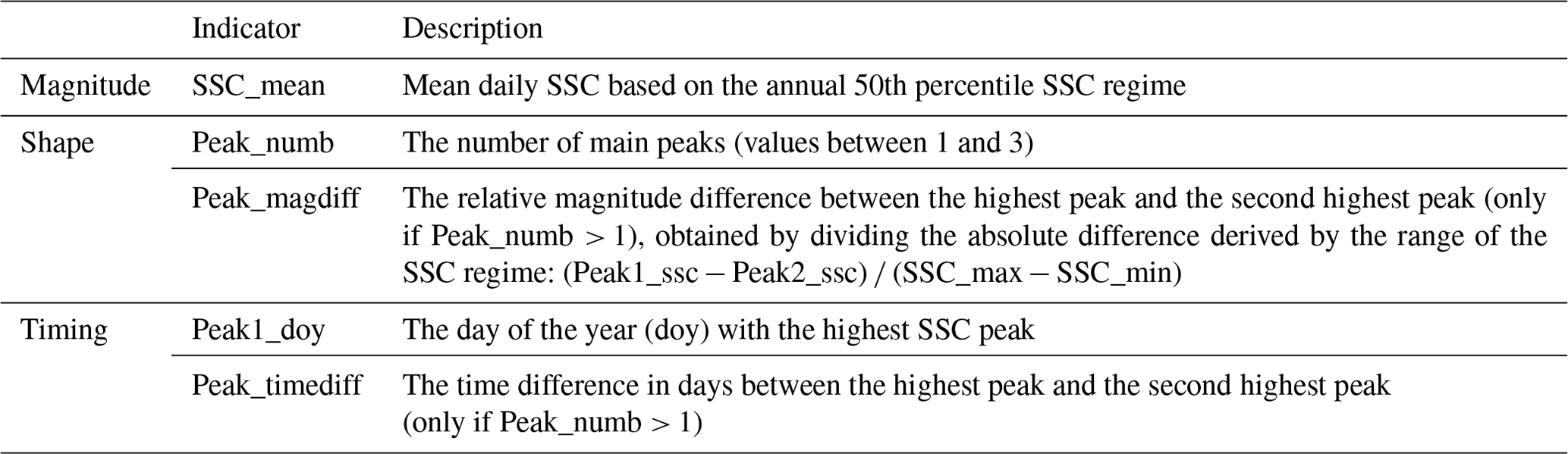
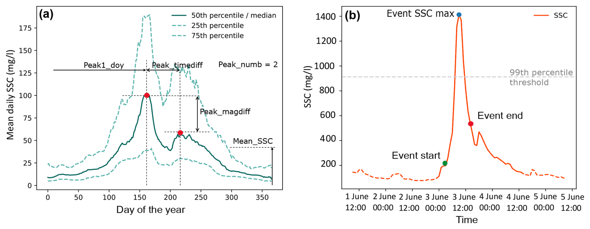
The median annual SSC regime is defined as the 50th percentile of mean daily SSC, smoothed over a 30 d time window to limit the sensitivity of the annual SSC regime to single values. Next, we selected five indicators that are able to capture the variations in the magnitude, shape, and timing of the annual SSC regime, referred to as MST indicators (Table 1 and Fig. 1a). The magnitude is represented by the median annual SSC per catchment (SSC_mean). Shape indicators include the number of peaks (Peak_numb) and the relative magnitude difference between the highest and second highest peak (Peak_magdiff). Timing indicators include the day of the year (Peak1_doy) on which the highest peak occurs and the time difference in days between the highest and second highest peak (Peak_timediff). The main peaks were identified automatically with the scipy.signal.find_peaks package (Virtanen et al., 2020) based on three criteria: peaks only occur above the 75th percentile of the annual SSC regime; the minimal horizontal distance between peaks is 30 d (1 month); and the peak prominence, which “measures how much a peak stands out from the surrounding baseline of the signal and is defined as the vertical distance between the peak and its lowest contour line” (Virtanen et al., 2020). In our case, the peak prominence is catchment specific and defined as 5 % of the SSC range ($\mathrm{0.05}\times (\mathrm{SSC}\mathrm{\_}\max -\mathrm{SSC}\mathrm{\_}\min )$). These parameters for peak identification were selected after visual inspection, with at least one peak being identified per SSC regime and without selecting too many additional peaks that did not contribute to the overall shape. The number of identified peaks varied from one to three peaks per annual SSC regime. For the catchments with multiple peaks, we also calculated the time lag and relative magnitude difference between the highest and second highest peaks. When the time difference (Peak_timediff) has a positive value, the highest peak happens earlier in the year than the second highest peak and vice versa.

Table 1 Overview of the five selected MST indicators that reflect the magnitude, timing, and shape of the median annual SSC regime per catchment.

Figure 1 (a) Visual overview of the five selected MST indicators (explained in Table 1) in relation to the median annual SSC regime of one example catchment. (b) SSC event (with event start and end), where the SSC max exceeds the 99th percentile threshold.

2.3.2 Hierarchical clustering based on SSC regime indicators

We applied hierarchical clustering to cluster the catchments based on their MST indicators. Clustering started by computing the Euclidean distance matrix using the matrix of $n=\mathrm{38}\times \mathrm{5}$ standardized MST indices (Python package sklearn.preprocessing.StandardScaler). Next, we used a hierarchical clustering algorithm (Python package sklearn.cluster.AgglomerativeClustering), which allows for non-elliptical clusters, and the Ward variance minimization algorithm, which minimizes the total within-cluster variance (Ward Jr., 1963), to identify clusters of similar SSC regimes. Finally, we optimized the number of clusters (k) by applying the silhouette score and the elbow method and validated the clustering based on a visual inspection of the dendrogram, keeping in mind the interpretability of the clusters. A sensitivity analysis showed that this clustering approach is robust and that removing single or multiple catchments does hardly influence the clustering results. Furthermore, a comparison with clusters derived by k-means clustering showed that the final clusters identified are relatively stable, regardless of the choice of the clustering technique.

2.3.3 Interpretation of variation in SSC regimes based on static catchment characteristics

For the interpretation of the three SSC regime clusters, we selected a number of physiographic catchment characteristics and hydrometeorological attributes (Sect. 2.2.1) that may be able to explain the spatial and seasonal variations in annual SSC regimes in mountain rivers. To better compare these characteristics among the different catchments, we used area-independent values, such as percentages (e.g. % forest cover) and specific discharge (in mm d⁻¹). In addition, we normalized all catchment and hydro-meteorological attributes to be within the range 0–1 across all catchments. For each cluster, we identified the most important catchment characteristics that are able to explain the spatial variation between different annual SSC regimes. The most important characteristics are those that clearly differ for the selected clusters and thus support the clustering. Finally, we also compared the annual regimes of the main transport processes (precipitation, glacial melt, snowmelt, and discharge) with the annual SSC regimes.

2.4 Spatial and temporal variations in extreme SSC events

To identify different types of extreme SSC events and to explain the spatial and temporal occurrence of these events, we performed several analysis steps which are discussed in more detail below: (i) detecting extreme SSC events; (ii) designing a classification scheme to distinguish between event types; and (iii) explaining the spatial and temporal differences between SSC event types based on seasonally varying characteristics, event characteristics, and antecedent conditions.

2.4.1 Detection of extreme SSC events

Extreme SSC events, i.e. episodic peaks of suspended sediment concentration, can be defined in different ways. While there is no commonly used definition for SSC extreme events, the peak-over-threshold method is widely used to extract extreme events (Skålevåg et al., 2024; Hamshaw et al., 2018; Haddadchi and Hicks, 2021; Blöthe and Hoffmann, 2022). In this study, we defined SSC extreme events as events for which the peak value exceeds a locally defined 99th percentile threshold (Fig. 1b). We identified the start of the event based on a rapid increase in the slope of SSC prior to the SSC peak (the increase in slope (Δ mg L⁻¹) is larger than the difference between the 50th and 75th percentiles of SSC for that catchment (mg L⁻¹)). The end of the event is defined as the time when the SSC drops below 0.4 times the SSC peak value. We also tested and compared other definitions, where the end of the event was equal to crossing the 90th percentile or was determined based on the decrease in slope. However, a sensitivity analysis showed that the choice of the exact definition had a limited effect on the total number of events selected (Fig. S5 and Table S3). When the end of one event and the start of the next event are less than 12 h apart, these events were merged into one event because we assumed that these events share the same drivers. We have deliberately chosen to make the selection of SSC events independently of discharge because such an approach also enables the selection of extreme SSC events during low-flow periods. Events with missing SSC or hydro-climatic data are removed. Since daily snowmelt and ice melt data were only available until the end of 2019, this means that we did not include extreme events that occurred after this date. Our approach led to the extraction of 2398 SSC extreme events across the entire study domain, with, on average, 64 events per catchment (min = 10, max = 143).

2.4.2 Classification of extreme events based on their dominant transport process(es)

To distinguish between different types of extreme events, we developed a classification scheme that identifies the most important driver(s) of each event. The three hydro-climatic processes that are most important for sediment transport to the river are erosive rainfall, snowmelt and glacial melt (Costa et al., 2018a). We assumed that each event is caused by either one or two out of these main transport processes. Inspired by the event-based classification of flood generation processes by Stein et al. (2020), we developed a classification scheme for extreme SSC events that assigns each event to one out of nine event types (Fig. 2). The most dominant transport process(es) per event is (are) determined based on the total rainfall, snowmelt, and glacial melt during the 24 h prior to the SSC peak of the event. Costa et al. (2018a) found that a 1 d time lag is the most relevant time lag for predicting SSC for the Rhône catchment. We tested this time lag on a selection of events and found that this short time lag aligns well with the fast response time of our catchments. Furthermore, we distinguished between high- and low-intensity precipitation as two different driving processes because soil erosion by runoff depends on rainfall intensity (Parsons and Stone, 2006; Mohamadi and Kavian, 2015). Precipitation is considered to be high intensity if the maximum hourly precipitation during the 24 h time window exceeds the catchment-specific 99th percentile threshold of hourly precipitation. All other precipitation values are considered to be low intensity. According to our definition, an event had two dominant transport processes (e.g. precipitation and snowmelt driven) if both precipitation and snowmelt contributed more than one-third of the total water input. The threshold of one-third was chosen to allow for a maximum of two dominant processes per event. A lower threshold could result in the selection of all three drivers for an event, but information about which of the drivers is the most dominant would be lost. A sensitivity analysis showed that higher thresholds (of up to $\mathrm{1}/\mathrm{2}$) result in a larger number of events with only one dominant transport process. Because we were also interested in events with compounding drivers, we used the one-third threshold.

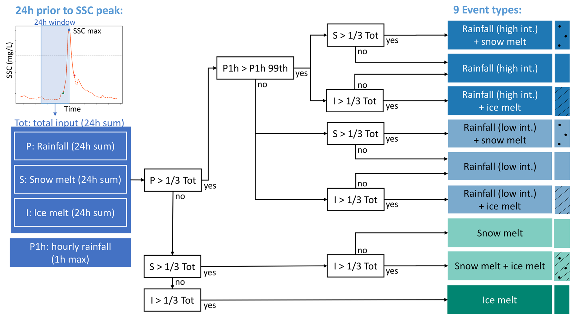
Figure 2 Decision tree used to categorize extreme SSC events into one out of nine predefined event types. The most dominant transport process(es) is (are) determined based on the fraction of total rainfall (P), snowmelt (S), and ice melt (I) (also referred to as glacial melt) compared to the total sum of P, S, and I (Tot) during the 24 h prior to the SSC peak of the event. Precipitation is classified as high intensity (high int.) if the maximum hourly precipitation (P1h) during the 24 h period exceeds the catchment-specific 99th percentile threshold of hourly precipitation. Otherwise, it is classified as low intensity (low int.).

2.4.3 Event characteristics and antecedent conditions analysed per event type

To learn more about the differences and similarities between the nine event types, we also looked at the spatial and temporal distribution of the event types across the Alps, the effect of antecedent conditions, and whether events belonging to the same event type share the same event characteristics. Event characteristics include event duration; mean and maximum event SSC; specific suspended sediment yield (sSSY) (t km⁻²); and event complexity, defined as the number of peaks in the SSC between the start and end of the event (Fig. 1b). We also calculated the sSSY event fraction out of the mean annual sSSY per catchment as an indicator of the extreme nature of the event in terms of the sediment load transported. In addition, we monitored important seasonally varying antecedent conditions during the 2 d prior to the SSC event, such as the mean snow cover and the soil moisture in the catchment, which control sediment availability.

Finally, we investigated the role of long-term catchment memory in terms of sediment availability in the development of extreme events. As a proxy for sediment memory, we compared the long-term cumulative sSSY prior to each event with the catchment-specific mean annual cumulative sSSY curve (for a detailed explanation, see Fig. S6 in the Supplement). For each day of the year, we determined whether the cumulative sSSY was above or below the mean annual sSSY curve. If the cumulative sSSY was below the mean (equating to a negative deviation), less sediment than usual had been transported during that season, and, therefore, more sediment may be available for mobilization during upcoming events. If the cumulative sSSY was above average (equating to a positive deviation), more sediment than usual had already been transported by previous events, which may have led to sediment depletion in the catchment and limited sediment availability for the next events. To make this index comparable among catchments, we standardized the deviation of the long-term cumulative sSSY from the catchment-specific mean annual sSSY curve by dividing it by the catchment annual mean cumulative sSSY.

3 Results

3.1 Large variation in median SSC among catchments

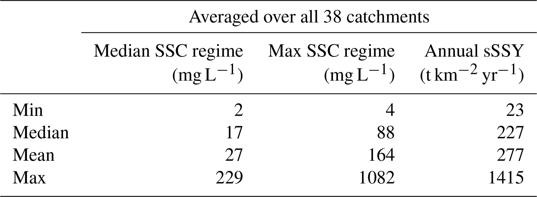
We observe a large variation in median SSC among the different catchments, with some catchments showing a median SSC which is 100 times greater than the one of other catchments even though all catchments are located in the same mountain range (Table 2). The median SSC varies from 2 to 229 mg L⁻¹ between the 38 catchments, with a mean SSC value of 27 mg L⁻¹. The mean annual sSSY varies from 23 to 1415 t km⁻² yr⁻¹, again with a difference of 2 orders of magnitude. The mean annual sSSY averaged over all 38 catchments is 277 t km⁻² yr⁻¹. The catchment with the largest median SSC and sSSY is the Vent catchment located in the Ötztal (Austria). This catchment has the highest mean elevation (2889 m a.s.l.) and a glacier cover of 30 % and is know for its high sediment output (Schmidt et al., 2022; Skålevåg et al., 2024). The catchment with the lowest median SSC is located at the foots of the northeastern Austrian Alps, with a mean catchment elevation of 938 m a.s.l. The large spatial variability allows us to investigate the causes of variation between catchments. To do this, we group the catchments into different clusters and analyse these clusters separately.

Table 2 Statistical description of the variation in the annual SSC regime (median and maximum) and cumulative annual sSSY among the 38 catchments.

3.2 Three types of annual SSC regimes

Our hierarchical clustering approach identified three main types of annual SSC regimes based on the magnitude, the shape, and the timing of the peak(s) (Fig. 3a–c): SSC regimes in cluster 1 (n=12) have two or multiple peaks, where the highest peak occurs at the end of spring and earlier in the year than the second highest peak; SSC regimes in cluster 2 (n=7) generally have one main peak, which occurs in mid-summer; and SSC regimes in cluster 3 (n=19) show an opposite shape compared to cluster 1, with the highest peak occurring later in the year than the second highest peak. The number of peaks and the timing of the first peak are the most important indicators for dividing the annual SSC regimes into these clusters, while the magnitude of the SSC regime (median SSC) is considered to be the least influential for clustering the catchments.

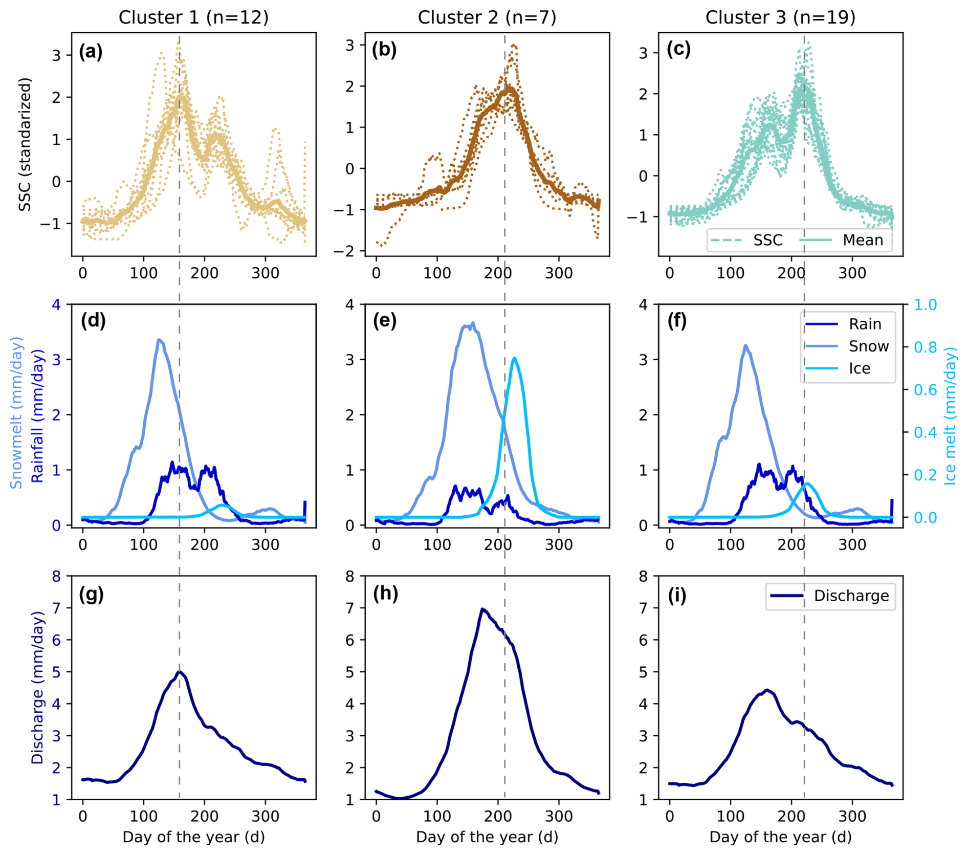
Figure 3 The median SSC regimes (standardized by removing the mean and scaling to unit variance) can be grouped into three different clusters: (a) cluster 1 (n=12), (b) cluster 2 (n=7), and (c) cluster 3 (n=19). The dashed lines show the regimes for the n individual catchments that belong to that cluster, and the bold line is the mean of all catchments per cluster. Panels (d), (e), and (f) show the mean annual regimes of precipitation, snowmelt, and glacial melt (in mm d⁻¹) averaged over all catchments within a cluster. The mean annual discharge regime over all catchments within a cluster is given in panels (g), (h), and (i). The vertical dashed grey lines spanning panels indicate when peak SSC occurs.

The catchments belonging to the three different SSC clusters are characterized by substantially different catchment characteristics (for an important subset, see Fig. 4a–h, and for the full overview, see Fig. S7). The catchments that belong to cluster 2 can be described as high-elevation, small mountain catchments because they are characterized by high mean elevation and slope, a high fraction of glacier coverage, high mean daily snowmelt and glacial melt, and a high fraction of sand (dark-brown boxplots in Fig. 4a–h). The effect of reservoirs is limited, and none of the catchments are located downstream of big lakes (Fig. S7). The catchments belonging to clusters 1 and 3 have quite similar catchment characteristics (beige and turquoise boxplots in Fig. 4a–h). Compared to those in cluster 2, they have a larger area, a lower mean elevation, and a higher fraction of clay and silt. The catchments in cluster 1 have, in general, a smaller fraction of precipitation that falls as snow, and the day of the year on which the catchment is completely snow-free happens earlier in the year than for the catchments in cluster 3. The fraction of highly erodible geology (such as unconsolidated sediments) is higher in catchments belonging to cluster 1, while the catchments in cluster 3 have a larger fraction of low-erosion geology (e.g. plutonic rocks, carbonate sedimentary rocks, acid volcanic rocks). Finally, a larger fraction of the catchments in cluster 1 than in cluster 3 are located upstream of lakes and reservoirs (Fig. S7).

The subtle differences between catchments in clusters 1 and 3 become more pronounced when we compare the annual SSC regimes with the mean annual regimes of precipitation, snowmelt, and glacial melt per cluster (Fig. 3d–f). Catchments with a single-peak SSC regime (cluster 2) are characterized by late snowmelt (as high mean elevation results in a late melting season), immediately followed by a significant input from glacial melt. The catchments in clusters 1 and 3 also receive significant snowmelt, but the melting starts at least 1 month earlier in the year than for catchments in cluster 2. The first peak in SSC for clusters 1 and 3 is mostly aligned with the first peak of rainfall. The largest difference between the catchments of clusters 1 and 3 is the amount of glacial melt during late summer. In catchments belonging to cluster 3, the glacial meltwater peak perfectly coincides with the second and highest SSC peak of the annual SSC regime. In catchments belonging to cluster 1, this increase in SSC during peak glacial melt is also visible but much weaker than for those in cluster 3. In terms of annual peak discharge (Fig. 3g–i), catchments in cluster 1 show peak discharges that are approximately simultaneous with the peak SSC, while peak discharge for catchments in cluster 3 is out of phase with the SSC peak. The spatial distribution of the different catchments across the Alps (Fig. 4i) supports the above findings. Catchments belonging to cluster 2 are mainly located in the higher Alpine region (with one exception being located in eastern Austria). The catchments of cluster 3 follow a clear line from east to west and are bounded to the north and south by the less mountainous catchments of cluster 1.

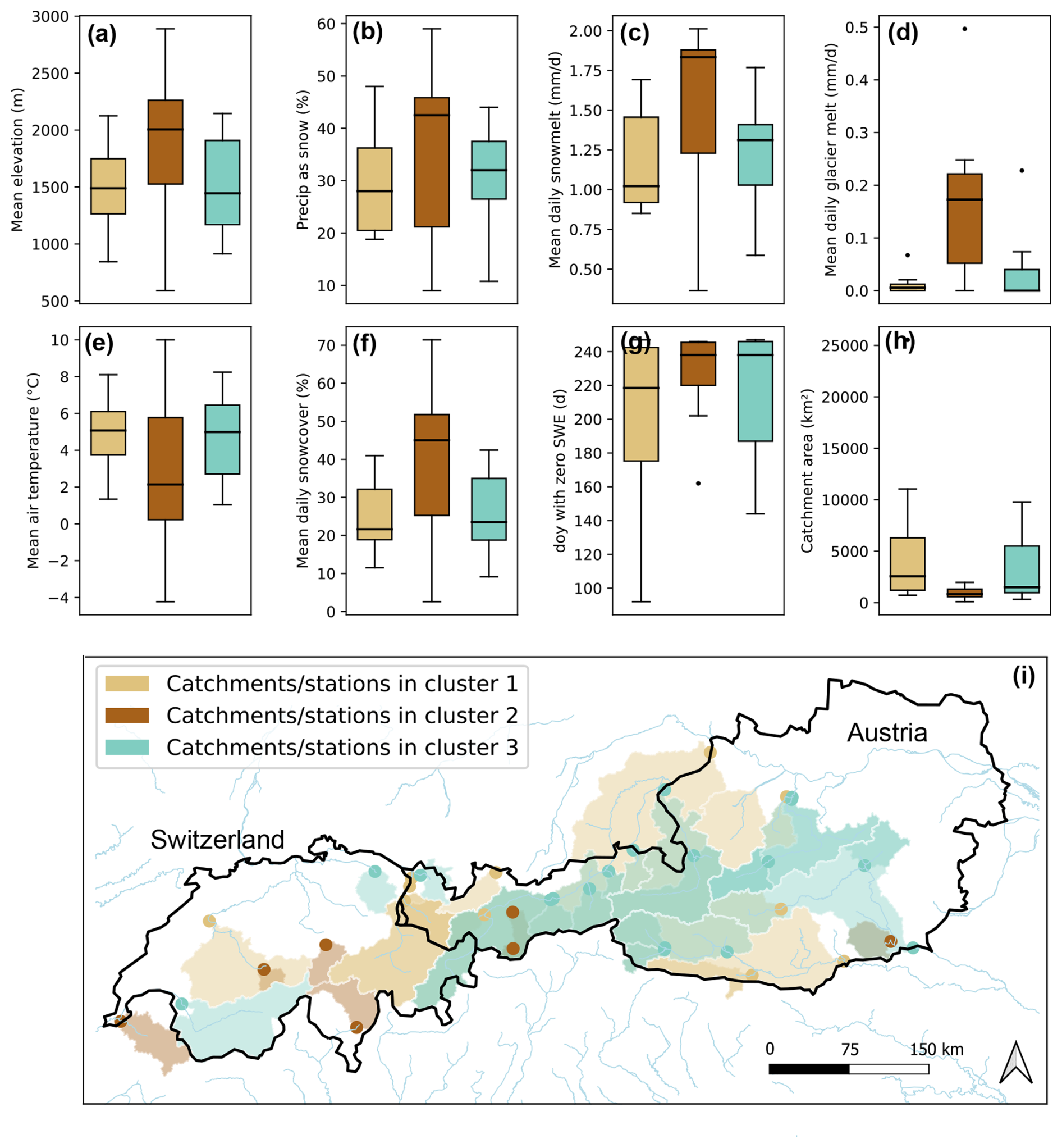
Figure 4 Panels (a)–(h) illustrate eight static catchment characteristics and their distribution across the three different clusters and within each cluster (the internal distribution is visualized by the boxplots). Panel (i) maps the spatial location of the (nested) catchments over Switzerland and Austria.

The magnitude of the SSC regime, although not used as such to split the catchments into the three above-mentioned clusters, has a moderate correlation (Pearson correlation coefficient > 0.5) with a number of catchment characteristics (Fig. S8 in the Supplement). The median SSC has a moderate positive correlation with the mean daily snowmelt (0.67), mean daily snow cover (0.67), catchment elevation (0.64), runoff ratio (0.60), sand fraction (0.58), fraction of precipitation that falls as snow (0.57), fraction of glacier coverage (0.55), and mean daily glacial melt (0.49). A negative correlation is found between the median SSC and the fraction of forest cover (−0.64), mean daily soil moisture (−0.58), fraction of silt and clay (−0.58), and mean daily air temperature (−0.58). These findings suggest that higher median SSC values should, in general, be expected in higher-elevated catchments that have a large contribution of snow and ice.

3.3 Temporal and spatial occurrence of the nine event types

In total, we extracted 2398 extreme SSC events, of which rainfall is by far the most dominant driver. In total, 85 % of the events are purely caused by either high- or low-intensity rainfall (1562 events (65.1 %) and 506 events (21.1 %)) (Fig. 5a and c). Those rainfall-driven events occur all year round but with a higher frequency during summer. Snowmelt-driven events are restricted to the melting season and occur only during late spring and autumn, and their timing is also dependent on catchment elevation. The same is valid for events that are caused by glacial melt, which only occur during July and August, when the snow cover on glaciers is minimal and the glacier becomes susceptible to melting. In total, 11 % of the events are (partly) snowmelt driven, and only 3.1 % are (partly) glacial melt driven.

The proportion of snowmelt- and glacial-melt-dominated events is significantly higher for high-elevation and partially glacierized catchments, which belong to cluster 2 based on the annual SSC regime clusters. In these catchments, snowmelt- and glacial-melt-dominated events account for almost 35 % of all events (Fig. 5b). In contrast, lower-elevation and larger catchments (clusters 1 and 3) show far fewer melt-dominated events (< 10 % out of all events).

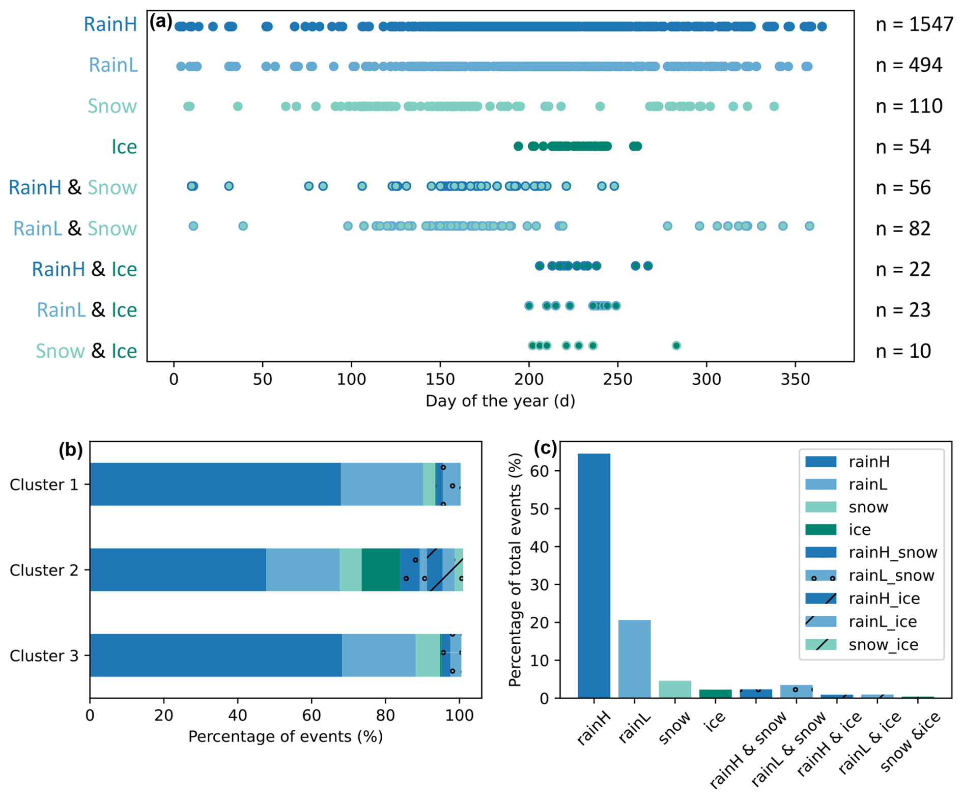
Figure 5 (a) Seasonality of occurrence of the nine event types: high-intensity rainfall (rainH), low-intensity rainfall (rainL), snowmelt (snow), glacial melt (ice), or a combination of two of the above mentioned transport processes. The total number of events is 2398. (b) Proportion of event types for each of the three annual SSC clusters. (c) Percentage of events per event type compared to the total number of observed events.

3.4 Event type characteristics

The event characteristics, such as the event maximum SSC, the area-specific suspended sediment yield (sSSY), and the sSSY event fraction out of the annual mean sSSY, vary greatly among the different event types (Fig. 6 and Fig. S8 in the Supplement). A total of 9 out of the 10 most extreme events, with the highest peak SSC, occurred in summer and are caused solely by high-intensity rainfall (peak SSC = 118 g L⁻¹ and sSSY event fraction = 0.33, averaged over the 10 most extreme events) (Fig. 6a). Similarly, the events with the highest sSSY and sSSY event fraction are also caused by high-intensity rainfall (Fig. S9a in the Supplement). However, when we look at the median of all events per event type, other event types result in higher peak SSC (Fig. 6j) or high sSSY event fractions (Fig. S9j in the Supplement). On average, the highest peak SSC values are caused by events with compounding drivers, namely those that are caused by a combination of glacial melt and high-intensity rainfall (median peak SSC of 5.5 g L⁻¹). On average, events caused by glacial melt alone lead to the second highest suspended sediment concentrations (median peak SSC of 4.2 g L⁻¹), the highest specific yields (median sSSY of 32 t km⁻² per event), and the second highest fraction of event sSSY (median sSSY event fraction of 0.03). Other event characteristics, such as the mean duration of events and the event complexity (number of peaks per event), are less informative as they do not clearly stand out for single event types. All events have a relatively short duration of less than 1 d, with a mean duration of 17 h.

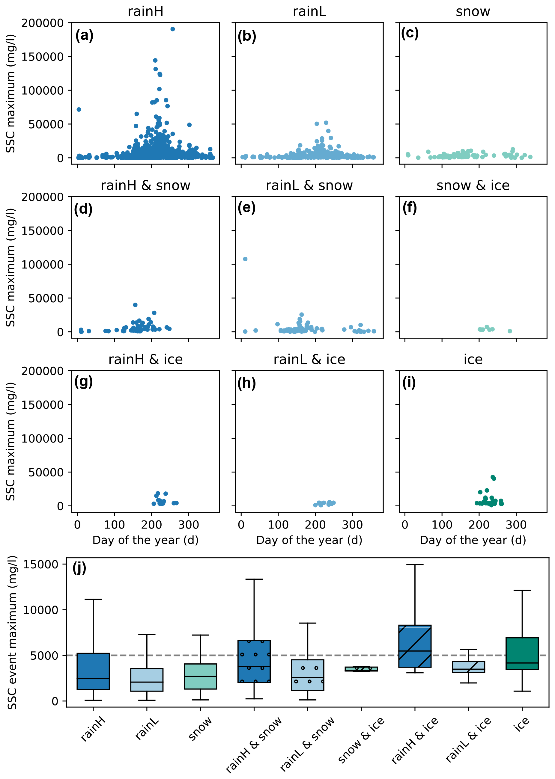
Figure 6 Relationship between event magnitude (peak SSC) and generation processes. Panels (a)–(i) illustrate the variation in peak SSC (including outliers) over time per event type. Panel (j) illustrates the distribution of peak SSC (without outliers) for each event type, with the median value being represented by a horizontal grey line.

In addition to the characteristics of the events, we also considered the antecedent conditions, such as the liquid volumetric soil moisture and snow cover, during the 2 d prior to the event. In general, the majority of events occur when snow cover is minimal or absent (Fig. 7a). However, a more detailed examination of the various event types provides additional insights (Fig. S10 in the Supplement). Events that are partly or entirely driven by glacial melt occur only when the snow cover has disappeared or is at least less than 30 %. In contrast, snowmelt events require the presence of a snowpack, and extreme SSC events occur under both limited and extensive snow cover. Events driven by a combination of rainfall and snowmelt are most prevalent when the snow cover is between 10 % and 30 %. However, some particularly severe events have been observed with a snow cover of 40 % to 70 %. Despite the occurrence of some of the most extreme events with exceptionally high peak SSC values under conditions with minimal snow cover, no clear pattern or relationship between snow cover and SSC could be identified.

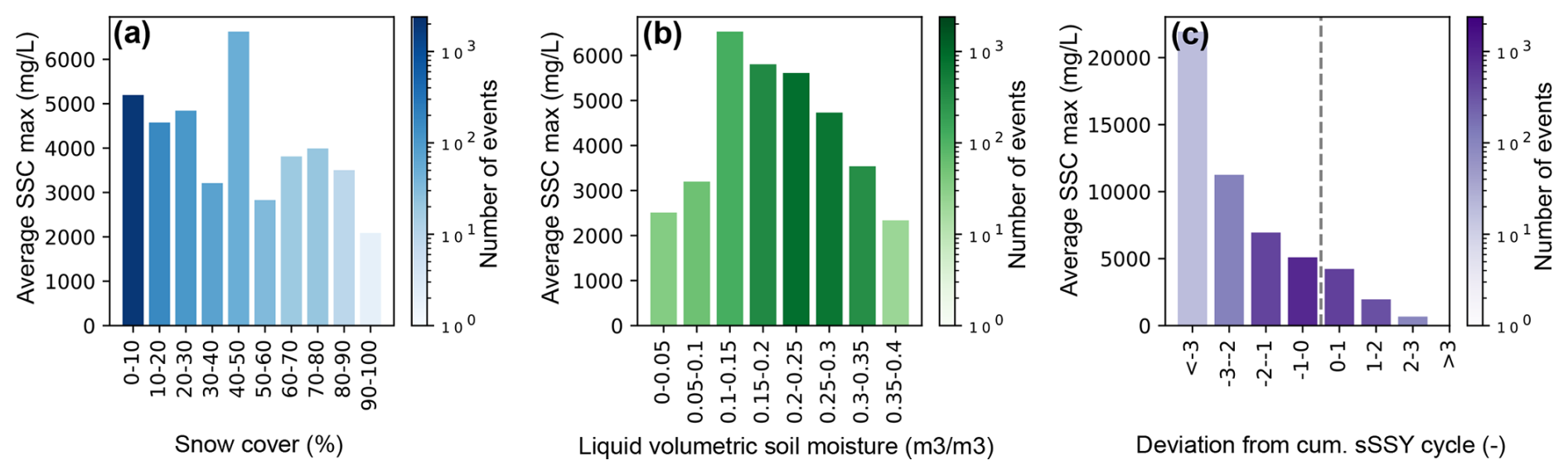
Figure 7 Antecedent conditions prior to the extreme SSC events are given for (a) snow cover, (b) liquid volumetric soil moisture, and (c) the deviation of the daily cumulative sSSY from the annual mean cumulative sSSY regime. Per interval, the bars show the peak SSC averaged over all of the events that belong to each of the intervals. The colour saturation is an indication of the number of events (in log scale) that belong to each interval. Dark colours mean that more events belong to that interval. Snow cover prior to the event can vary from 0 % to 100 %. The liquid volumetric soil moisture generally varies from 0 to 0.4 m³ m⁻³. The deviation from the cumulative sSSY regime can be either negative (indicating more sediment availability than usual) or positive (indicating potential sediment depletion).

The majority of events occur when liquid volumetric soil moisture lies between 0.2 and 0.3 m³ m⁻³ (Fig. 7b). The maximum liquid volumetric soil moisture typically ranges from 0.2 m³ m⁻³ in sandy soils to 0.4 m³ m⁻³ in clay soils. A more detailed overview per event type is visible in Fig. S11 in the Supplement, which shows some discrepancies in the relation between peak SSC and soil moisture between the event types. Glacial melt events predominantly occur under liquid volumetric soil moisture values of 0.2–0.25 m³ m⁻³, with occurrences at lower or higher soil moisture levels being rare. In high-elevation and partly glacierized catchments, where glacial melt events are most frequently observed, the soil is typically composed of a higher proportion of sand, which may contribute to the observed lower liquid volumetric soil moisture. In the case of rainfall-driven events, the most severe events, with the highest peak SSC, take place under antecedent soil moisture values between 0.1–0.2 m³ m⁻³, which implies rather dry conditions. The statistical analysis revealed no significant correlations between soil moisture and SSC.

The proxy for catchment memory and sediment availability, designed as the deviation of the long-term cumulative sSSY from the mean annual cumulative sSSY regime, shows that more (severe) events occur when the deviation is negative (Fig. 7c). A negative deviation indicates a situation in which the transport of sediments during the period prior to the event was below the expected level, suggesting that sediment availability is not a limiting factor for riverine sediment transport. More negative deviations result in larger observed peak SSC. Similar patterns are observed for rain- and snow-dominated events, an exception being (partly) glacial melt events (Fig. S12 in the Supplement). A significant number of glacial melt events occur when the deviation is slightly positive (Fig. S12f–i in the Supplement).

4 Discussion

4.1 Mean SSC regimes

Our results show that the annual SSC regimes can be divided into three clusters (Fig. 3a–c), where the catchments in each cluster share similar catchment attributes (Fig. 4a-h) and seasonal regimes of snowmelt and glacial melt (Fig. 3d–i). This suggests that, in addition to precipitation, the amount of glacial melt and the magnitude and timing of snowmelt strongly control the shape of the annual SSC regime (number of peaks) and the timing of SSC peaks (Fig. 3d–i). This is particularly evident when examining catchments in cluster 3, for which the occurrence of the glacial meltwater peak perfectly coincides with the second but highest SSC peak in the annual SSC regime (Fig. 3c and f). The importance of snowmelt and glacial melt is confirmed by the analysis of the catchment characteristics (Fig. 4a–h). The most important characteristics explaining seasonal sediment dynamics are those that influence the magnitude and timing of snowmelt and glacial melt, for example, the presence of glaciers (even if they cover only a small part of the catchment), catchment elevation, the proportion of precipitation falling as snow, and catchment area. The importance of meltwater for SSC has already been highlighted by multiple other studies; for example, Costa et al. (2018b) showed that glacial melt produces the highest SSC per unit runoff, Buter et al. (2022) showed that glacial melt results in even higher sediment concentrations than snowmelt, and Li et al. (2024) showed that the suspended sediment yield of glaciated catchments can be an order of magnitude larger than that of glacier-free catchments.

The high concentration of suspended sediment in glacial meltwater can be explained by the importance of the glacier and glacier forefields as a sediment source and temporary storage. Glacial abrasion on the bedrock causes erosion, and these sediments get transported by subglacial channels. However, these channels need time to develop at the start of the ablation season before they become very effective (Swift et al., 2005). In addition, a lot of material is stored in the recently deglaciated moraines and the glacial forefields (Moore et al., 2009). The braided stream network in this deglaciated terrain can be highly dynamic and therewith has an important influence on sediment availability (Mancini et al., 2024). This means that areas above 2500 m a.s.l., which are characterized by glacier tongues, bare-rock surfaces, and recently deglaciated areas, are crucial for sediment generation in high-altitude catchments (Schmidt et al., 2022). A sudden release of suspended sediments has been observed when areas above 2500 m become snow-free and when the sediments are no longer protected from mobilization by the snow cover (Schmidt et al., 2022).

In addition, our results show that the relationship between SSC and discharge is not straightforward because the annual discharge regime is completely out of phase with the SSC regime in some catchments (Fig. 3), particularly in catchments that belong to cluster 3 and are characterized by significant glacial melt input during late summer. Discharge has long been considered to be one of the key predictors of SSC, and the relation between discharge and suspended sediment concentration forms the basis of the well-known sediment rating curves and hysteresis analyses (Walling, 1977). However, other studies have recently shown that this relationship has been overvalued (Costa et al., 2017; Schmidt et al., 2023; Skålevåg et al., 2024). Sediment rating curves are characterized by a large variability of observations around the regression curve, which can span 1 or several orders of magnitude, and they tend to underestimate (overestimate) SSC during high (low) discharge (Walling, 1977; Horowitz, 2003; Asselman, 2000). One of the major limitations is that the SSC–discharge relationship does not explicitly address the sources of sediment and their activation by different hydro-climatic forcings. Costa et al. (2017) have shown that a sediment source perspective using hydro-climatic forcing (rainfall, snowmelt, and glacial melt) is more appropriate to explore sediment dynamics than traditional discharge-based rating curves. In line with this, Zhang et al. (2021) introduced a sediment–availability–transport (SAT) model that captures the time-varying sediment availability. Their results are consistent with ours as our results suggest that the origin of water entering the river system is more informative for understanding the mean annual SSC regime than the absolute magnitude of discharge alone.

Even though forcing and transport processes were expected to be among the key determinants of the annual SSC regime, it is still surprising that catchment characteristics related to sediment availability, spatial connectivity, geology, and soil type did not appear to be more important for explaining the variation in the annual SSC regime among catchments (Fig. S6). The catchments belonging to the three clusters of annual SSC regimes did show some mutual differences in the fraction of clay, silt, and sand, and we observed a slightly larger fraction of highly erodible geology in catchments in cluster 1 compared to those in cluster 3. However, these differences were small, and they did not significantly affect the timing and shape of the SSC regime. We did observe some correlations between a few catchment characteristics and median SSC, but, again, characteristics related to snowfall, snow cover, ice, and catchment elevation were more important descriptors of SSC behaviour than geology-related characteristics. While SSC is controlled by the depletion and replenishment of different sediment sources over longer timescales (Doomen et al., 2008), we hypothesize that these processes were found to be less relevant in our study because our analyses focused on the mean annual scale.

Looking at the spatial variability of median SSC and sSSY values across catchments, we found that values can vary greatly across locations (Table 2). Median SSC values range from 2.11 to 229 mg L⁻¹ per catchment, while the mean annual sSSY varies from 19 to 1226 t km⁻² yr⁻¹. These values are in line with those previously described in the literature, where sSSY values vary between 100–1000 t km⁻² yr⁻¹ as mountainous regions are generally characterized by high sediment yields (Blöthe and Hoffmann, 2022; Vanmaercke et al., 2011; Bogen, 2008; Borrelli et al., 2014; Hinderer et al., 2013; Mano et al., 2009). In addition, Panagos et al. (2015) predicted a mean soil loss rate of 527 t km⁻² yr⁻¹ for the alpine climate zone (Alps, Pyrenees, and southern Carpathians) due to the combined effect of rainfall erosivity and topography. One of the highest sediment discharge rates in Europe was recorded in the Italian Central Apennines, with a specific yield of 3235 t km⁻² yr⁻¹ (Borrelli et al., 2014), due to very active geomorphological processes such as gully, rill, bank, and channel erosion and re-entrainment of landslide sediments. Such extremely high levels have not been recorded in our catchments.

4.2 Extreme SSC events

From the event classification, we conclude that rainfall is by far the most dominant driver of extreme SSC events (Fig. 5c), which shows that slightly different processes are important for controlling extreme events compared to annual SSC regimes. In total, 85 % of the events are purely caused by either high- or low-intensity rainfall (1562 events (65.1 %) and 206 events (21.1 %)) (Fig. 5c). This dominant role of precipitation in causing extreme SSCs has also been highlighted in other studies (Schmidt et al., 2022; Mano et al., 2009; Lana-Renault et al., 2007; Blöthe and Hoffmann, 2022). The process of rainfall-driven splash erosion, which is followed by the generation of surface overland flow on hillslopes, results in the delivery of fine sediment to the river network. Therefore, precipitation is also being increasingly considered to be a valuable input in various SSC modelling approaches, such as the process-based rating curve of Costa et al. (2018a), the extended sediment rating curve of Wolf et al. (2023), and the machine learning model of Aires et al. (2023). Given that rainfall affects a much larger area than glacial melt or even snowmelt and occurs at higher intensities, it was anticipated that rainfall would emerge as the most dominant driver. On the other hand, for snow- and glacier-dominated catchments, the number of snowmelt and glacial melt events was larger and could make up to 35 % of all events in these catchments. This is consistent with the existing knowledge on runoff generation processes in mountainous snow-dominated catchments, where snowmelt and glacial melt are significant contributors to overland flow and river discharge (Muelchi et al., 2021).

From the comparison of mean SSC peak values among the different event types, we conclude that events that are partly or entirely dominated by glacial melt result in relatively high SSCs (Fig. 6j). These findings are in line with the existing literature stating that glacial melt has a significantly higher suspended sediment input per unit of runoff compared to snowmelt and rainfall (Buter et al., 2022; Costa et al., 2017, 2018b). Events with compounding drivers, specifically those resulting from the interaction of glacial melt and high-intensity rainfall, show the highest peak SSC values on average (median peak SSC of 5.5 g L⁻¹ and mean peak SSC of 7.7 g L⁻¹). However, the 10 highest SSC values in our data set are predominantly associated with high-intensity rainfall events during the summer season, with values reaching up to 118 g L⁻¹. Although these observed SSC values are extremely high, concentrations of the same order of magnitude have been found by other authors (Schmidt et al., 2022) and in other Alpine catchments (Mano et al., 2009). Actually, a significant number of 573 extreme SSC events (24 % of all extreme events) in our data set cause SSC peak values above 5 g L⁻¹, which are very likely to be harmful or lethal to a large number of aquatic species, including trout, salmon, and aquatic invertebrates (Newcombe and Macdonald, 1991; Kemp et al., 2011; Collins et al., 2011). Such high levels of SSC also degrade drinking-water quality; lower the transparency of water and limit the penetration of sunlight into the water; lead to a degradation of the habitat quality for spawning fish; and clog the gills of fish and other aquatic organisms, which can lead to death (Kemp et al., 2011).

On average, the highest event sSSY is found for events driven by glacial melt (52 t km⁻²) or a combination of glacial melt and high-intensity rainfall (42 t km⁻²) (Fig. S9 in Supplement). During such events, large volumes of sediment produced by glacial erosion and temporarily deposited into proglacial systems are likely to be mobilized and transported downstream by high-intensity precipitation (Li et al., 2024). If we compare the event sSSY with the mean annual sSSY of the catchment, we see that these extreme events transport, on average, 2 % of the catchment’s annual sSSY. However, some high-intensity rainfall events can transport up to 20 % or 60 % of the annual sSSY. Similar results were found for the Vent catchment in the Ötztal, where individual summer rainstorm events can account for up to 26 % of the annual sSSY in just over 24 h (Schmidt et al., 2022).

During some of the most sediment-productive events, some headwater catchments transported more than 4 times the average annual sSSY in just 6 to 8 d. Further investigation showed that these events were related to two major storm and flood events that occurred in Europe: the large flooding in central Europe in early June 2013, with more than 300 mm of precipitation over 4 d on the northern side of the Alps, resulting in large flooding in the Upper Danube basin (Blöschl et al., 2013), and the storm, “Vaia”, that hit southern Austria on 28 October 2018, characterized by extreme accumulated precipitation of up to 850 mm in 3 d (Giovannini et al., 2021). Further downstream, the sSSY of these flood events still accounted for up to 150 % to 280 % of the average annual sediment yield. Such high sediment yields are only possible in combination with landslides and river floods, when all the sediment in and near the riverbed gets activated. This was the case for both the 2013 and 2018 events (Blöschl et al., 2013; Giovannini et al., 2021). While these events with very high sediment yield play a significant role in soil loss within a catchment, a high sediment yield does not necessarily lead to a high sediment concentration as long as it is combined with high discharge (Zheng et al., 2021).

The relationship between antecedent conditions and extreme suspended sediment concentration (SSC) events is complex. Notably, some of the highest peak SSCs and specific suspended sediment yields (sSSYs) occurred during periods of high soil moisture and limited snow cover (Fig. 7) as saturated soils are generally more prone to landslides, and snow-free soils are less protected from erosion (Godt et al., 2009; Hamshaw et al., 2018). At the same time, rainfall during previously wet conditions does not always lead to high SSCs. Moderate rainfall can also lead to high runoff without a corresponding increase in SSC. If the whole catchment contributes to the runoff, sediment concentrations may not increase due to dilution effects (Lana-Renault et al., 2007) if the sediment input is proportional to the water input. In contrast to wet soils, dry soils can also be prone to erosion at the onset of rainfall events due to hydrophobicity, splashing, and surface sealing (Zambon et al., 2021). Our observations indicate that high-intensity rainfall events often result in more severe SSCs under relatively dry conditions compared to under wet ones (Fig. S11 in the Supplement). A final complicating factor, which we did not explicitly consider in this study, is the potential effect of changes in land use on soil moisture, discharge, and erosion. All of these contrasting signals complicated efforts to establish a clear correlation between SSC and soil moisture (Fig. 7b). Furthermore, we noticed that glacial melt occurs only when the snow cover has disappeared or is at least smaller than 30 %. This could be a model artefact as it is consistent with how glacial melt is represented in the PCR-GLOBWB 2.0 model, which assumes that glaciers only start melting when they are no longer covered (and protected) by snow. This assumption is supported by the findings of Schmidt et al. (2022) – who showed that subglacial sediment sources are inactive as long as areas above 2500 m (including glacier tongues) are frozen or snow-covered – and of Kormann et al. (2016).

Our proxy for catchment memory, designed based on the long-term deviation of cumulative sSSY, shows a positive relationship between the availability of sediment sources and event peak SSC. We observe more events with higher peak SSC when sediment resources are still abundant (Fig. 7c). This is in line with our expectations as the presence of abundant sediment sources creates favourable conditions for the occurrence of extreme SSC events. It should be noted, however, that no relationship was visible when we reset the catchment memory each winter, implying that sediment stores build up and empty over several years. In our case, deviations in sediment storage developed and were tracked throughout the time series (10–12 years).

The combination of greater sediment availability and sufficient forcing (e.g. high-intensity rainfall or snowmelt) results in larger observed peak SSCs. The only exception are those events that are (partly) driven by glacial melt. These events also occur frequently during conditions in which more sediment than usual has already been transported prior to the event (Fig. S12f–i in the Supplement). One potential explanation for this is that events driven by glacial melt rely on a different sediment source compared to those driven by snowmelt and precipitation, namely sediments from the glacier and its forefields (Mancini et al., 2024). Consequently, the transportation of sediments during glacial melt is independent of the availability of sediments in other areas within the catchment. However, this is inconsistent with the fact that this method makes use of the catchment-specific annual cumulative sSSY regime, which already accounts for the different sediment sources within a catchment. It is possible that these events occurred during an exceptional period of glacier retreat or glacier motion that exceeded the annual average as rapid glacier retreat and areas of recently deglaciated terrain reveal effective sediment sources (Moore et al., 2009; Swift et al., 2005).

4.3 Limitations and generalizability

The results presented are associated with uncertainties, which result from a combination of uncertainties inherited from the underlying data and methodology. One important data-related limitation is the uncertainty in the turbidity–SSC relationship. Despite the many efforts by the Swiss and Austrian hydrographic services in collecting bi-weekly manual SSC samples, it is difficult to reconstruct the relationship between turbidity and SSC reliably. The non-linear regression model attempts to represent the relation of SSC with turbidity, but the actual variability in the relationship between turbidity and SSC will likely be more stochastic as it is influenced by the varying characteristics of the sediments in suspension (particle size, shape, density, and colour) (Gippel, 1995; Merten et al., 2014) and is also strongly dominated by mass wasting (Battista et al., 2022). Nevertheless, the turbidity–SSC relationship is currently the most applied and accepted method to derive high-resolution SSC time series described in the literature and has been used by Costa et al. (2018a), Pellegrini et al. (2023), Stott and Mount (2007), and Thollet et al. (2021), among others. Because of the uncertainty in the turbidity–SSC relationship, we removed a few implausible outliers and decided to aggregate the data from 10 and 15 min to mean hourly values. Before analysing the annual SSC regimes, we had to smooth the time series over a 30 d window to account for the relatively short time series. A further limitation of this study is the limited availability of SSC data, which has resulted in a relatively small sample size. At the same time, comprehensive large-sample studies are scarce. By analysing 38 rivers across the Alps, we believe that our analyses capture the most important processes and their variability in space and time.

Other uncertainties can be related to the methodology, e.g. the hierarchical clustering approach, the definition of extreme events, and the event classification scheme developed. For the clustering of the annual SSC regimes, we applied a hierarchical clustering algorithm. As each clustering method has its advantages and disadvantages, we performed a sensitivity analysis comparing the results of hierarchical clustering with the ones resulting from k-means clustering. This showed that the clusters identified are relatively stable, regardless of the choice of the clustering technique. However, a well-known disadvantage of clustering in general is that the selected indicators can strongly influence the final clusters. We deliberately selected indicators that were able to capture the shape of the SSC regime rather than the variation in the magnitude or the synchronicity with the discharge regime. This choice is reflected in the clusters identified, which differ mostly in terms of the number and timing of the main peaks.

For the detection of extreme SSC events, we applied a peak-over-threshold approach, which is widely used (Skålevåg et al., 2024; Hamshaw et al., 2018; Haddadchi and Hicks, 2021; Blöthe and Hoffmann, 2022). At the same time, the definition of extremes necessarily entails some degree of subjectivity and arbitrary decision-making. Instead of using the 99th-percentile threshold, a lower threshold could have been selected (for instance, the 90th percentile). This would have resulted in the extraction of more events, but these would be less extreme. Furthermore, the methodology employed to define the start and end of an event is inherently subjective. The definition of the start of extreme SSC events is rather straightforward as it is characterized by a sudden and pronounced increase in SSC that is easily detectable by a change in the slope. However, determining the end of the event was more challenging. We tested and compared three different methods within the framework of a sensitivity analysis, including the use of the slope, another fixed threshold, or the decrease in SSC relative to the SSC peak (Fig. S5 in the Supplement). The duration and the calculated sSSY of the event varied slightly depending on the selected method. However, the sensitivity analysis demonstrated that our primary results and conclusions remain unaffected by such changes in the definition (Table S3 in the Supplement).

The classification scheme that we presented here is relatively straightforward to apply and is therefore explainable. It requires only a few inputs (hourly precipitation and daily snowmelt and glacial melt) and is based on the relatively well-understood processes of sediment transport, while more complex processes of sediment availability are ignored for simplicity. Our event classification relies on our input data, and, as the snow and glacial melt data are evaluated over the larger Alpine domain, they might be more uncertain in smaller catchments and on shorter timescales. However, general melt patterns are well-represented. Since our classification focuses on the dominant processes, it is less sensitive to smaller-scale uncertainty and increases our trust in our classification. We show that the method is applicable to catchments of different sizes, and the absence of glaciers does not have a detrimental impact on the results. Given that the threshold for differentiating between dominant transport processes is set at one-third, one would expect a considerable number of precipitation–snowmelt-dominated events in catchments without glacial melt but with substantial snowmelt contributions. However, our analysis indicates that this is not a concern as the number of precipitation–snowmelt-dominated events is relatively limited, even in non-glaciated catchments. Our event classification differs from existing classification techniques, such as those proposed by Millares and Moñino (2020) and Skålevåg et al. (2024), which both rely extensively on the SSC–discharge relationship. In fact, the analysis of the annual SSC regimes has led us to conclude that discharge is a poor predictor of SSC in some catchments, thereby supporting the decision to select only hydro-climatic drivers for the classification scheme.

Our choice of methods and the use of a large sample of catchments contribute to the generalizability of our results. The clustering of SSC regimes and the event classification scheme have been designed to be transferable to other catchments and regions. Thus, this study does not only improve our understanding of the complex hydrological–sedimentary response in the studied catchments but also opens the door to further large-sample studies focusing on SSCs. Finally, our results and conclusions might be generalizable to other mountain regions with similar characteristics because the catchments considered in our data set covered a large variety of catchment characteristics (mean catchment elevation from 590 to 2889 m, glacier cover from 0 % to 33 %, and fraction of precipitation falling as snow from 0 to 0.34).

4.4 Implications of findings and outlook

The importance of snowmelt and glacial melt for both seasonal and event SSC dynamics suggests that climate change might affect sediment concentrations and fluxes in Alpine rivers in the future. There is evidence that glacier retreat results in a potential increase in suspended sediment concentrations and fluxes, and this effect can last for decades and centuries in small alpine watersheds (Moore et al., 2009; Buter et al., 2022). However, a long-term decline in suspended sediments delivered from glacial sources is anticipated under future climate change scenarios since the area of glacier cover and glacier erosion will decrease, and glacier forefields will stabilize (Moore et al., 2009; Mancini et al., 2024). Future projections of sediment export for two catchments in the Ötztal suggest a decrease in sediment export already in the coming decades and imply that “peak sediment” has already passed (Schmidt et al., 2024). This is in line with findings by Freudiger et al. (2020), who concluded that glacier peak water has already been reached in most of the catchments in the Swiss Alps in the past decades and will be reached in all catchments during the first half of this century, independent of the emission scenario. In addition, for non-glaciated catchments, such as the Illgraben Valley, one of the most geologically unstable regions of Switzerland, studies also suggest a future decline in sediment transport (Hirschberg et al., 2021). Although future climate conditions are expected to favour an increase in the sediment transport capacity in this valley, a reduction in sediment supply produced by frost weathering may limit debris flow activity and actual sediment transport.

In addition to alterations in glacial coverage, future changes in snow seasonality and reduced snow accumulation and coverage are also expected to influence sediment availability in catchments and concentrations in rivers (Maruffi et al., 2022). When sediment sources are covered by snow, they are protected from erosion and not connected to the river system, resulting in a reduction in SSC during winter (Schmidt et al., 2022). Consequently, shorter periods with snow and generally reduced snow cover will lead to longer periods with potentially increased connectivity of sediment sources to the river, which may lead to higher SSC. Nevertheless, we hypothesize that an extended period during which sediments can be transported may also cause a depletion of sediment sources, resulting in lower SSCs later in the year.

Likewise, the impact of future precipitation on changes in sediment concentration remains incompletely understood, particularly in combination with sediment availability. Heavy and extreme precipitation events in the summer months will occur with greater frequency and intensity (Wood and Ludwig, 2020; Martel et al., 2020), and such occurrences have the potential to cause significant erosion and an elevated annual yield (Schmidt et al., 2024). However, as a consequence of dilution, high precipitation and high discharge do not necessarily result in the highest suspended sediment concentrations (Lana-Renault et al., 2007). While these alterations in the contribution of rain, snowmelt, and glacial melt will result in a shift in the timing of runoff and discharge seasonality, their impact on the SSC regime remains uncertain. Our observation-based insights into the relationship between melt processes and SSCs suggest future changes in SSC behaviour. However, targeted modelling and field experiments are needed to better understand the whole process chain – from weathering to erosion, sediment storage, and sediment transport – and to make reliable projections of future SSC.

5 Conclusions

In this paper, we identified the main factors influencing the spatial and seasonal variability in the annual SSC regime and the occurrence of extreme SSC events in 38 catchments in the Alpine region. Our results demonstrate that the annual SSC regime and extreme SSC events in small mountain catchments are substantially influenced by snow and ice, which is in contrast to low-elevation and large catchments, where liquid precipitation is more important. The presence of glaciers and the magnitude and timing of snowmelt are important factors influencing the annual SSC regime and controlling the timing of peak SSC, while geology- and soil-related catchment characteristics and the annual discharge regime appear to have a smaller influence. Furthermore, we present a novel classification scheme to categorize extreme SSC events into nine different event types. Our analysis of 2398 extreme SSC events indicates that rainfall is the primary driver of SSC extremes, accounting for 85 % of all events. This shows that slightly different processes are important for controlling extreme events compared to annual SSC regimes. However, in high-elevation and partly glaciated catchments, up to 35 % of the events are still attributable to snowmelt and glacial melt. Events with compounding drivers, namely glacial melt and high-intensity rainfall, result in the highest sediment concentrations and area-specific yields. Events driven by glacial melt have a specific yield of, on average, 52 t km⁻², which means that 10 of these short-term extreme events account for the transport of the total annual sediment yield of an average catchment. Moreover, a considerable proportion of the extreme SSC events (24 % of the total) resulted in peak SSC values exceeding 5 g L⁻¹, which can have detrimental effects on aquatic ecosystems. These findings highlight the importance and impact of such events on the water quality in alpine rivers and give an indication of soil loss due to water erosion.