Assimilating ESA CCI land surface temperature into the ORCHIDEE land surface model: insights from a multi-site study across Europe

Land surface temperature (LST) plays an essential role in water and energy exchanges between the Earth's surface and atmosphere. Recent advancements in high-quality satellite-derived LST data and land data assimilation systems present a unique opportunity to bridge the gap between global observational data and land surface models (LSMs) to better constrain the water and energy budgets in a changing climate. In this vein, this study focuses on the assimilation of the ESA CCI-LST product into the ORCHIDEE LSM (the continental part of the Institut Pierre-Simon Laplace Earth system model) with the aim of optimizing key parameters to improve the simulation of LST and surface energy fluxes. We use the land data assimilation system for the ORCHIDEE model (ORCHIDAS) to conduct a series of synthetic twin data assimilation experiments accounting for actual data availability and uncertainty from ESA CCI-LST to find an optimal strategy for assimilating LST. Here, we test different strategies of assimilation, notably investigating (i) two optimization methods (a random search technique and a gradient-based technique) and (ii) different ways to assimilate LST using the only raw data and/or different characteristics of the LST diurnal cycle (e.g. mean daily, daily amplitude, maximum and minimum temperatures, and morning and afternoon gradients). Upon identifying the optimal approach, we use ORCHIDAS to assimilate ESA CCI-LST data across 34 European sites provided by the Warm Winter database. Our results demonstrate the effectiveness of assimilating 3 h CCI-LST data in ORCHIDEE over a single year in 2018, thereby improving the accuracy of simulated LST and fluxes. This improvement, assessed against CCI-LST and in situ observations, reaches up to a 60 % reduction in the root-mean-square deviation, with a median decrease of 20 % over the entire validation period (2009–2020). Furthermore, we evaluate the effectiveness of optimized parameters for application at larger scales using the median of optimized parameters per vegetation type across sites. Notably, the performance for both LST and fluxes exhibits consistent stability over the years, comparable to using site-specific parameters, and indicates a significant improvement in the modelled fluxes. Future work will be focused on refining the utilization of the observation uncertainties provided by the ESA CCI-LST product (e.g. decomposed uncertainties and spatio-temporal variability) in the assimilation process.

1 Introduction

Surface heat fluxes, particularly sensible and latent heat fluxes, exchanged between the land surface and the atmosphere, play an essential role in the climate system as well as in numerous hydrological, meteorological, and agricultural applications (Bateni et al., 2013; Caparrini et al., 2004; Olioso et al., 1999). Land surface models (LSMs) have been developed to simulate the complex interactions between the land surface and the atmosphere, offering valuable insights into the quantification and comprehension of energy and water fluxes within the system. While simulations from LSMs may accurately represent ecosystem state variables and observed fluxes under certain conditions, significant temporal and spatial biases still occur. These biases are attributed to simplifications in the representation of the processes governing energy and mass transfers, errors in the input data (atmospheric forcing, vegetation, and soil spatial information), and errors in the model parameterization.

In recent decades, efforts to address these discrepancies have explored the potential of using land surface temperature (LST) observations through optimization or assimilation procedures in land surface monitoring (Boni et al., 2001; Coudert et al., 2008; Crow et al., 2003; Demarty et al., 2005; Ghent et al., 2010; Margulis and Entekhabi, 2003; Olioso et al., 1999; Ridler et al., 2012). In fact, LST is a key variable in LSMs because it reflects the coupled energy and water budgets, which are linked by evapotranspiration (Benavides Pinjosovsky et al., 2017; Coudert et al., 2008; Ridler et al., 2012). Therefore, LST observations have proven to be of great value not only for assessing water and energy fluxes but also for refining their estimation.

Recent advances in remote sensing technology and derived LST products provide a valuable benchmark for the evaluation and optimization of LSMs. Particularly noteworthy is the progress in high-quality satellite-derived LST information that integrates measurements from diverse satellite sensors, including both geostationary and polar orbit platforms, such as the ESA CCI-LST product (Hollmann et al., 2013; Veal et al., 2022). These advancements have yielded global LST products with enhanced spatial and temporal resolutions, thus expanding their potential utility and compatibility with LSMs.

A number of studies have been previously conducted to parameterize LSMs using LST data (e.g. Boni et al., 2001; Coudert et al., 2008; Crow et al., 2003; Demarty et al., 2005; Ghent et al., 2010; Margulis and Entekhabi, 2003; Olioso et al., 1999; Ridler et al., 2012). Coudert et al. (2008) highlighted the advantages of incorporating the dynamics of the LST diurnal cycle into model parameter calibration compared with the direct use of raw LST observations. This is explained by the fact that the use of raw LST values, which are prone to inaccuracies in their estimation, can introduce errors in the optimization process (Coudert et al., 2006; Demarty et al., 2005). This issue can be especially exacerbated when comparing different satellite products (Coudert et al., 2008). In this respect, the merged ESA CCI-LST product derived from various satellite thermal infrared sensors allows one to assess the diurnal cycle characteristics, given its harmonization between LST satellite products, while providing a global product with associated uncertainties. The availability of a global LST product with its corresponding uncertainties is an important asset for the data assimilation (DA) processes in LSMs, as knowledge of observations and model uncertainties is crucial to obtain realistic model–data fits in DA.

DA offers a valuable framework for integrating measurements and models, weighting the sources of error in both, to generate a statistically optimal and dynamically consistent estimation of the evolving system state (Margulis and Entekhabi, 2003). Some studies have focused on the assimilation of LST into LSMs with the aim of enhancing simulations of LST and water and energy fluxes (Bateni et al., 2013; Benavides Pinjosovsky et al., 2017; Caparrini et al., 2003; Ghent et al., 2010; Lu et al., 2017; Meng et al., 2009; Sini et al., 2008). DA approaches can also be used to estimate model parameters (Rayner et al., 2019), either independently or together with the model state (Bateni and Entekhabi, 2012; Moradkhani et al., 2005). Therefore, DA techniques have been widely used to control LSM state variables and/or for parameters optimization (e.g. Bacour et al., 2023; Moradkhani et al., 2005; Peng et al., 2011; Raoult et al., 2016; Rayner et al., 2005; Santaren et al., 2007). DA techniques allow us to calibrate LSMs against observational data, providing best-fit internal parameters and associated uncertainty ranges compared with default parameters.

Recent advancements in both high-quality satellite-derived LST data and land DA systems offer a promising opportunity to bridge the gap between observations and LSMs and, thus, to better constrain the land surface water and energy budgets. In this vein, this study focuses on assimilating the merged LST data from the ESA CCI product into the ORganizing Carbon and Hydrology In Dynamic EcosystEms (ORCHIDEE) LSM, the continental component of the IPSL (Institut Pierre-Simon Laplace) Earth system model. Concurrently, there is a growing availability of in situ measurement sites providing estimates of sensible and latent heat fluxes at high temporal resolution, primarily from FLUXNET observations (FLUXNET, 2016). Recognizing the value of both data sources, this study aims to leverage the complementary information from the CCI-LST product (see Sect. 2.1.1) and the Warm Winter database (Warm Winter 2020 Team and ICOS Ecosystem Thematic Centre, 2022). We achieve this by assimilating CCI-LST data at selected sites from the Warm Winter database and utilizing flux observations as independent validation data. Our primary objective is to investigate whether LST observations from the ESA CCI product have the potential to improve ORCHIDEE simulations of water and energy fluxes, accounting for their frequency and measurement uncertainties. To this end, we seek to identify an optimal assimilation strategy by testing different approaches, including assimilating raw LST observations and specific characteristics of the LST diurnal cycle (e.g. daily maximum, amplitude, and morning and afternoon gradients). We investigate whether assimilating observed characteristics of the LST diurnal cycle can provide additional constraints compared with assimilating raw LST data alone. We initially conducted a series of synthetic twin DA experiments to select the optimal assimilation strategy. We then implemented the selected DA strategy across 34 European sites provided by the Warm Winter database using ESA CCI-LST data extracted at each site, assessing the effectiveness of the assimilation process with respect to improving LST and surface energy flux simulations.

2 Materials and methods

2.1 Data

2.1.1 LST observations from the ESA CCI product

In this study, we use the merged infrared (IR) Climate Data Records (CDRs) from the LST Climate Change Initiative (CCI) project by the European Space Agency (ESA) (Hollmann et al., 2013; Veal et al., 2022), referred to as CCI-LST. The merged IR CDRs include all available IR geostationary sensor data and IR low-Earth-orbit (LEO) sensor data over the period from 2009 to 2020, delivered with a 3 h temporal resolution and a global spatial resolution of 0.05°. The IR geostationary sensor includes the Imager on the Geostationary Operational Environmental Satellite (GOES) platforms, the Spinning Enhanced Visible and Infrared Imager (SEVIRI) aboard the Meteosat Second Generation platforms, and the Japanese Advanced Meteorological Imager (JAMI) on the Multi-functional Transport Satellite (MTSAT) platform. The LEO data come from the Advanced Along-Track Scanning Radiometer (AATSR), the MODerate resolution Imaging Spectroradiometer (MODIS) aboard Terra and Aqua, and the Sea and Land Surface Temperature Radiometer (SLSTR) aboard Sentinel-3A and Sentinel-3B.

The CCI-LST observations have an associated total uncertainty estimate derived from different error components. These error components correlate on various spatial and temporal scales and include the following: (i) random uncertainties weakly correlated (like random noise in the satellite data), (ii) locally correlated atmospheric uncertainties (related to atmospheric conditions), (iii) locally correlated biome or surface uncertainties, (iv) large-scale systematic uncertainties (related to calibration of the satellite sensor), and (v) locally correlated LST correction uncertainties (for intercalibration or time corrections). The total uncertainty is obtained from the sum of each uncertainty component in quadrature (i.e. the square root of the sum of squares), which is used in this study to prescribe observation errors in the assimilation process (Sect. 2.3).

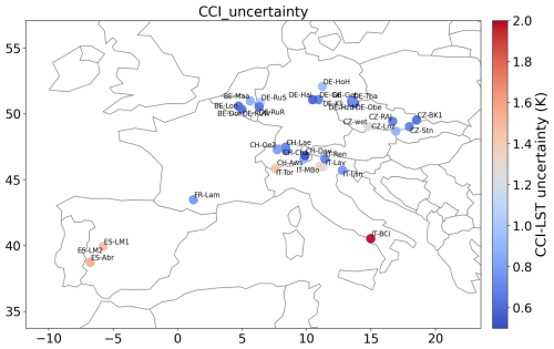
Figure 1 illustrates the median of 3 h CCI-LST uncertainties during the optimization year (2018) at the corresponding 0.05° CCI-LST pixel over each of the 34 selected sites (detailed below). These uncertainties are used in the assimilation process as the observation error. The median LST uncertainties are, on average, 1.05 K across the 34 sites evaluated, ranging from 0.76 to 1.89 K for the DE-Kli and IT-BCi sites, respectively. It should be noted that the Mediterranean sites present larger uncertainties which ranged between 1.50 and 1.89 K. These larger values are mainly explained by the LST correction component, i.e. the (v) uncertainty component mentioned in the list above, which could be attributed to more complex surface conditions, such as heterogeneous land cover types.

Figure 1 Location of the eddy-covariance flux tower sites from the Warm Winter network. The median of the 3 h LST uncertainty from the ESA CCI product during the optimization year (2018) is represented at the corresponding CCI-LST pixel.

2.1.2 In situ observations

We use meteorological data and measurements of surface energy fluxes for the stations available in Europe from the Warm Winter database (Warm Winter 2020 Team and ICOS Ecosystem Thematic Centre, 2022). The sites used in this study are depicted in Fig. 1 and detailed in Table A1 (e.g. their location, data period, and vegetation and climate types). The Warm Winter network is chosen for its coverage of recent periods, which aligns with the CCI-LST period, and it represents the latest freely available dataset for the European Union. The meteorological data (air temperature, humidity, pressure, wind speed, rainfall and snowfall rates, and shortwave and longwave incoming radiation) at a 30 min time step are used as forcing for the ORCHIDEE model. The eddy-covariance measurements of latent heat (LE) flux and sensible heat (H) flux and measurements of net radiation (R_n) are also used to evaluate the performance of ORCHIDEE simulations, using default parameters and after optimization. We selected these 34 sites based on two criteria: (i) the dominant vegetation type accounting for more than 50 % of the corresponding ORCHIDEE grid cell and (ii) full data availability for the optimization year (2018) across all sites. We chose the year 2018 for two main reasons: (i) all sites have recorded observations during this year and (ii) there are drought events in Europe throughout certain periods. This selection enables the consideration of parameters associated with droughts in both the sensitivity analysis and potentially in the optimization process. The selected sites collectively represent 7 of the 15 plant functional types (PFTs) of ORCHIDEE, and the length of each observation record varies from 4 to 11 years (considering only the available period of CCI-LST data). Thus, the selection of 34 sites ensures a comprehensive representation of diverse land vegetation types, being as homogeneous as possible at the 0.05° resolution of the CCI-LST product.

2.2 The ORCHIDEE land surface model

The ORCHIDEE land surface model is designed to simulate exchanges of carbon, water, and energy between the land surface and the atmosphere, as detailed by Krinner et al. (2005). In this study, we use version 2.2, which has been developed at the IPSL (Institut Pierre-Simon Laplace, France) and contributed to Phase 6 of the Climate Model Intercomparison Project (CMIP6) in a coupled configuration with an atmospheric circulation model (Boucher et al., 2020). The ORCHIDEE model allows an implementation across a broad range of spatial scales – including grid point, regional, or global levels – and spans timescales ranging from 30 min to thousands of years.

The study employs a temporal resolution of 30 min intervals to model hydrological and photosynthetic processes and the energy balance. In contrast, slower components related to carbon allocation within plants, autotrophic respiration, leaf onset and senescence, plant mortality, and soil organic matter decomposition are treated at a daily time step. The hydrological model in ORCHIDEE discretizes the first 2 m of the soil column into 11 layers, each with increasing grid spacing progressing geometrically with a ratio of 2 (De Rosnay et al., 2002). The soil moisture at various levels is determined by solving the Richards equation, which models vertical water transfer in the unsaturated zone. The land surface in ORCHIDEE is characterized by 15 PFTs, including bare soil, which can coexist within a given grid cell. The yearly varying PFT maps are derived from the ESA CCI land cover products (Lurton et al., 2020; Poulter et al., 2015). In this study, the soil type is characterized by soil texture, for which ORCHIDEE uses the global soil map based on the Zobler soil classification (Zobler, 1999) reduced to three different textures. Except for phenology, the processes are described by generic equations for the different vegetation and soil types but with different parameters that are PFT-specific or soil texture-specific, respectively.

We implement ORCHIDEE at the site level using 30 min meteorological data measured at each of the 34 sites evaluated. A prior spin-up simulation was performed at each site to bring soil carbon pools, the vegetation state, and the soil moisture content to equilibrium. This procedure is applied by running ORCHIDEE for several hundred years and recycling the available forcing data with the present-day CO₂ concentration. A transient simulation (starting from the first year of measurement for each data stream) was then performed after each spin-up simulation, accounting for the secular increase in atmospheric CO₂ concentrations.

2.3 Parameter optimization methodology

2.3.1 Data assimilation framework

The ORCHIDEE Data Assimilation System (ORCHIDAS) has been extensively discussed in previous studies (Bacour et al., 2015; Bastrikov et al., 2018; Kuppel et al., 2012; Peylin et al., 2016; Santaren et al., 2014). This assimilation framework is built upon a variational Bayesian approach, optimizing ORCHIDEE parameters represented by a vector x. The optimization process involves iteratively minimizing a global cost function J(x) (Tarantola, 2005), assuming Gaussian errors for both observations and model parameters:

$$\begin{array}{}\text{(1)}& \begin{array}{rl}J\left(\mathit{x}\right)& ={\displaystyle \frac{\mathrm{1}}{\mathrm{2}}}\left[\left(H\right(\mathit{x})-\mathit{y}{)}^T{\mathbf{R}}^{-\mathrm{1}}(H\left(\mathit{x}\right)-\mathit{y})\right.\\ & \left.+{\left(\mathit{x}-{\mathit{x}}_{\mathrm{b}}\right)}^T{\mathbf{B}}^{-\mathrm{1}}\left(\mathit{x}-{\mathit{x}}_{\mathrm{b}}\right)\right],\end{array}\end{array}$$

where x is the vector of parameters to optimize and y is the vector of observations. The first part of the cost function measures the mismatch between the observations (y) and the corresponding model outputs (H(x)), whereas the second part represents the mismatch between the prior parameter values (x_b) and the optimized parameters x. T represents the transpose of the matrix. Both terms of the cost function are weighted by their prior covariance matrices: R and B for the observation and parameter errors, respectively. As the error covariance matrices are difficult to assess, they are neglected in this study; thus, R and B are diagonal, as in most studies. The observation errors for each site are prescribed as the median of CCI-LST uncertainty over the optimization year (2018) for the corresponding pixel and are illustrated in Fig. 1.

Two methods to minimize the cost function are tested in this study: a gradient-based algorithm and a random search algorithm (described below).

Gradient-based minimization algorithm: L-BFGS-B

We use the gradient-based L-BFGS-B (limited-memory Broyden–Fletcher–Goldfarb–Shanno algorithm with bound constraints; Byrd et al., 1995), referred to as BFGS, to iteratively minimize J(x). BFGS offers the advantage of considering bounds in parameter variations, enabling comparability with the genetic algorithm, and leveraging our existing knowledge of parameters. The algorithm requires the evaluation of J(x) and its gradient with respect to each parameter to explore the parameter space. In this study, the gradient is calculated with a finite-difference approximation, where we quantify the ratio between the alteration in model output and the adjustment in model parameter. The search ceases once the relative change in J(x) falls below 10⁻⁴ for five consecutive iterations. As gradient-based algorithms have the potential drawback of converging to local minima rather than to the global one (more likely in non-linear models), we run a set of independent assimilations initiated with 16 distinct random initial guesses for the parameter vector, as in Bastrikov et al. (2018). Although some issues may arise when using Gaussian assumptions in gradient-based minimization algorithms (MacBean et al., 2016), most parameter errors follow Gaussian distributions in the cases of ORCHIDEE (Santaren et al., 2007).

Random search minimization algorithm: genetic algorithm

The genetic algorithm (GA) method is derived from the principles of genetics and natural selection (Goldberg, 1989; Haupt and Haupt, 2004) and performs a stochastic search over the entire parameter space. Parameter vectors are considered to be chromosomes, with each gene corresponding to a given parameter. The algorithm works iteratively, filling a pool of a given number of chromosomes at each iteration. The initial pool is created with randomly perturbed parameters. A sequence of operations (selection, crossover, and mutation) then simulates population evolution, which is described for ORCHIDAS in Santaren et al. (2014) and Bastrikov et al. (2018). We adopt a GA configuration identical to that in Santaren et al. (2014), who experimented with various GA set-ups to identify the set-up yielding the smallest optimal cost function and requiring the fewest iterations. The configuration consists of a population of 30 chromosomes, a maximal number of iterations of 40, a crossover : mutation ratio of 4:1, a number of gene blocks exchanged during crossover of 2, and a number of genes perturbed during mutation of 1.

2.3.2 Sensitivity analysis and parameters to be optimized

We perform sensitivity analysis at each of the 34 sites assessed to determine which ORCHIDEE parameters have the most influence on the simulated LST and characteristics of the diurnal cycle. The selection of crucial parameters for optimization serves a dual purpose: it enhances computational efficiency in the optimization process and mitigates the risk of overfitting.

Table 1 ORCHIDEE parameters evaluated in the sensitivity analysis at the 34 sites: the model parameter name, descriptions, and default values are shown. The 11 sensitive parameters to be optimized over the selected site (ES-Abr) for the twin DA experiments are indicated in bold. For the twin experiments, absolute values for soil hydrology parameters are used, whereas scaling factors are applied to the 34 sites (values in parentheses) because they depend on soil type.

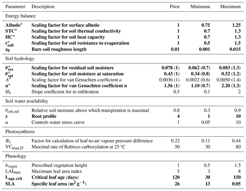
^* Scaling factor applied to an ORCHIDEE parameterization. Note that the scaling factor may involve more than a unique parameter in the model.

We use the Morris method (Morris, 1991) to assess the sensitivity of 19 parameters linked to ORCHIDEE LST simulations (detailed in Table 1). We implement this method because it is effective with relatively few model runs compared with other methods like the Sobol' sensitivity analysis (Sobol, 2001). Furthermore, the Morris method has been frequently utilized for parameter selection in ORCHIDEE (e.g. Abadie et al., 2022; Bastrikov et al., 2018; Raoult et al., 2021, 2023). The Morris method is a one-factor-at-a-time (OAT) method of sensitivity analysis that evaluates the relative importance of the parameters from the elementary effects (EE) of each parameter on model outputs. Basic statistics from multiple EEs in the parameter space allow us to build a ranking, which approximates well to a global sensitivity measure. This qualitative method requires only a small number of simulations, $(p+\mathrm{1})\times n$, where p is the number of parameters and n is the number of random trajectories generated. As the sampling strategy significantly impacts the Morris method, we apply the improved sampling strategy proposed by Campolongo et al. (2007) that is suited for models with a large number of parameters like ORCHIDEE. This strategy maximizes the dispersion of trajectories in the parameter space. In addition, the number of trajectories and levels (i.e. the sampling of the parameter space) can considerably impact the method and the selection of parameters to be optimized (Ruano et al., 2012). Therefore, we conducted a preliminary test to select the optimal n trajectories for the ORCHIDEE model by evaluating the Morris results by increasing n from 5 to 100 according to the position factor of the rankings proposed by Ruano et al. (2012). Based on this test, we use 20 trajectories and 10 levels for an optimal sampling of the parameter space. The Morris method applied to each site allows one to identify the most sensitive parameters for each site; these parameters are subsequently retained for the single-site optimization in the DA experiments (described in Sect. 2.4). An example of these outcomes is presented in Fig. B1 over a selected site in Spain (ES-Abr) for the twin DA experiments, whose identified parameters to be optimized are highlighted in bold in Table 1. The sensitivity analysis at the ES-Abr site required 400 simulations, $(\mathrm{19}+\mathrm{1})\times \mathrm{20}$. The mean (μ) and standard deviation (σ) for all of the trajectories are calculated to assess the overall importance of each parameter. We select the parameters with a normalized μ or normalized σ value higher than 0.2 in the twin experiment and at the rest of the sites. For the 34 sites, the same 19 parameters are evaluated in the sensitivity analysis, from which the number of selected parameters to be optimized ranges between 5 and 17, with one-third of the sites presenting 12 parameters to be optimized.

2.3.3 Selection of the DA experiment set-up

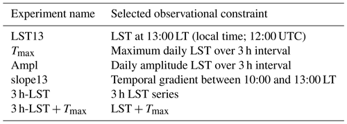
A series of synthetic twin DA experiments are tested over a selected site in Spain (ES-Abr) to understand the respective constraint brought by LST pseudo-observations as well as several characteristics of the diurnal cycle of LST and to evaluate their capability to improve ORCHIDEE simulations. The characteristics of the diurnal cycle of LST are estimated based on 3 h interval model outputs to be consistent with the 3 h frequency of CCI-LST data. The characteristics evaluated are daily LST amplitude, maximum LST, minimum LST, morning gradient (the slope between 10:00 and 13:00 LT, where LT denotes local time), and afternoon gradient (the slope between 16:00 and 19:00 LT). Additionally, we evaluate assimilating the LST at 13:00 LT, as the early afternoon is well-suited for detecting water stress (Lagouarde et al., 2019; Koetz et al., 2018). This is particularly relevant because the upcoming TRISHNA (Thermal infraRed Imaging Satellite for High-resolution Natural resource Assessment) mission will provide LST at 13:00 LT, a few hours later than other thermal missions widely used in recent decades for stress detection (e.g. Landsat, ASTER, and MODIS). Consequently, we aim to assess the potential impact of assimilating a single LST observation per day at this particular time. LST pseudo-observations and each derived characteristic of the diurnal cycle are assimilated separately, and different combinations are then considered, some of which are detailed in Table 2. All of the combinations tested are presented in Table S1 in the Supplement.

Table 2 Example of typical ORCHIDEE variables optimized in the DA experiments performed and used to determine the optimum strategy.

In each DA experiment, we optimize the 11 parameters selected from the sensitivity analysis carried out over the ES-Abr site for 3 h LST and each characteristic (parameters in bold in Table 1). The LST pseudo-observations for the DA experiments are generated by running the ORCHIDEE model using its default parameter values. A set of random values for the 11 parameters to be optimized is then used as the prior parameters in the optimizations. No uncertainties or model discrepancies are considered in these first LST pseudo-observations (unbiased by observational uncertainties) to allow us to directly assess the performance and convergence properties of the optimization schemes. In these DA experiments, the second term of the cost function (Eq. 1) was excluded to evaluate the role of observations. Therefore, we can conduct a direct comparison between the optimized parameters and the “true” parameters – set as the ORCHIDEE parameters by default – enabling the optimization process to freely recover these parameters and assess the accuracy of the optimizations.

We perform 16 independent runs for each DA experiment with 16 different first guesses randomly selected within the range of variation in the parameters, as in Bastrikov et al. (2018). The choice of 16 sets is a trade-off between computational cost and minimizing the risk of not converging toward a stable cost function minimum, as verified by Bastrikov et al. (2018). The DA experiments are tested using the BFGS and GA methods starting from the 16 sets of different first guesses. The 16 different first guesses are kept identical for all of the DA experiments (including between the BFGS and GA methods) to ensure the same first-guess values and to be consistent between DA experiments.

The prior uncertainty on the ORCHIDEE parameters is set to 15 % of the range of variation for each parameter. This error is set following preliminary DA tests over the ES-Abr site, where we explored different percentages of the range of variation as parameter errors. We found that a prior parameter error ranging between 10 % and 20 % of the range of variation emerges as optimal, exhibiting further improvements in fluxes after assimilating LST. Unlike the assimilation of actual CCI-LST data, where we used the errors provided with the LST product (see Sect. 2.3.4), the observation errors are defined as the mean-squared difference between the observations and the prior model simulations in the twin DA experiments, following Bastrikov et al. (2018).

The performance of the DA experiments is assessed in terms of their ability to (i) retrieve true parameter values and (ii) simulate the 30 min LST and turbulent fluxes from the posterior parameters. The performance is evaluated using the reduction in the root-mean-square difference (RMSD) between the prior and the posterior, as defined in Eq. (2). In addition, the performance is evaluated by comparing the posterior parameter values and against the true values, as estimated through the pseudo-observation tests.

$$\begin{array}{}\text{(2)}& {\mathrm{RMSD}}_{\mathrm{reduction}}=\left(\mathrm{1}-{\displaystyle \frac{{\mathrm{RMSD}}_{\mathrm{post}}}{{\mathrm{RMSD}}_{\mathrm{prior}}}}\right)\mathrm{100}\end{array}$$

For each DA experiment, independent of the observational constraint assimilated, the RMSD_reduction is estimated for the 30 min LST and turbulent flux (LE and H) simulations. This evaluation involves calculating the model–data fit between each posterior simulation using 16 different first guesses and the prior simulations (from an ORCHIDEE run with a unique set of prior parameters).

Based on the outcomes of the DA pseudo-data experiments, we select those showing the best results fitting the LST and turbulent fluxes. To evaluate the feasibility of assimilating the CCI-LST product, we consider its actual availability and uncertainties within the chosen optimal strategies. Thus, we implement a second set of twin DA experiments introducing some modifications. The LST pseudo-observations are filtered out with the actual availability of CCI-LST, thereby accounting for gaps in the time series resulting, for example, from cloudy conditions. Subsequently, these pseudo-observations are perturbed with Gaussian errors derived from their respective 3 h CCI-LST uncertainties. This refined approach ensures a more realistic representation of the assimilation process, considering both the real-world constraints and uncertainties associated with the CCI-LST data.

2.3.4 Assimilation experiments based on ESA CCI-LST data

Once the optimal DA strategy is selected (from the twin experiments at one site), it is implemented across the 34 European sites of the Warm Winter 2020 network for the year 2018. The parameters to be optimized are identified for each site from the sensitivity analysis described in Sect. 2.3.2. The performance is mainly evaluated via the RMSD reduction between the prior and the posterior ORCHIDEE simulations against CCI-LST and in situ energy flux (R_n, LE, and H) observations (described in Sect. 2.1). Additionally, we employ the decomposition of the mean-square error (MSE; Kobayashi and Salam, 2000) to gain deeper insights into which specific error components are improving or degrading. The MSE (i.e. the square of the RMSD) is decomposed into three components: the squared bias (SB), the lack of correlation weighted by the standard deviation (LCS), and the squared difference between standard deviations (SDSD). The three components are expressed as follows:

$$\begin{array}{}\text{(3)}& {\displaystyle }\mathrm{SB}={\left(\stackrel{\mathrm{‾}}{y_{\mathrm{sim}}}-\stackrel{\mathrm{‾}}{y_{\mathrm{obs}}}\right)}^{\mathrm{2}}\text{(4)}& {\displaystyle }\begin{array}{rl}\mathrm{LCS}=& \mathrm{2}\sqrt{{\displaystyle \frac{\mathrm{1}}{N}}\sum _{i=\mathrm{1}}^N{\left(y_{\mathrm{sim},i}-\stackrel{\mathrm{‾}}{y_{\mathrm{sim}}}\right)}^{\mathrm{2}}},\\ & \sqrt{{\displaystyle \frac{\mathrm{1}}{N}}\sum _{i=\mathrm{1}}^N{\left(y_{\mathrm{obs},i}-\stackrel{\mathrm{‾}}{y_{\mathrm{obs}}}\right)}^{\mathrm{2}}}(\mathrm{1}-r),\end{array}\text{(5)}& {\displaystyle }\begin{array}{rl}\mathrm{SDSD}=& \left(\sqrt{{\displaystyle \frac{\mathrm{1}}{N}}\sum _{i=\mathrm{1}}^N{\left(y_{\mathrm{sim},i}-\stackrel{\mathrm{‾}}{y_{\mathrm{sim}}}\right)}^{\mathrm{2}}}\right.\\ & {\left.-\sqrt{{\displaystyle \frac{\mathrm{1}}{N}}\sum _{i=\mathrm{1}}^N{\left(y_{\mathrm{obs},i}-\stackrel{\mathrm{‾}}{y_{\mathrm{obs}}}\right)}^{\mathrm{2}}}\right)}^{\mathrm{2}}.\end{array}\end{array}$$

Here, $\stackrel{\mathrm{‾}}{y_{\mathrm{sim}}}$ and $\stackrel{\mathrm{‾}}{y_{\mathrm{obs}}}$ are the means of simulations (y_sim,i) and observations (y_obs,i), respectively, and r is the correlation coefficient. The MSE decomposition provides valuable information on areas of improvement and potential limitations in the assimilation process.

The parameters optimized in 2018 are then used to evaluate ORCHIDEE simulations during the validation period from 2009 to 2020 (i.e. the CCI-LST period), where in situ observations are available. Additionally, we evaluate a unique set of parameters for each PFT from the previous site-specific optimized parameters in 2018. This is a key step in scaling parameter optimization, as broader-scale simulations (i.e. from regional up to global) require a unique set of parameters for each PFT. Thus, we calculate the median of optimized parameters across sites to evaluate the effectiveness of optimized parameters at larger scales. The median of generic parameters is computed across all sites, while PFT-specific parameters are computed for each PFT. Finally, we run ORCHIDEE with this unique parameter set for each PFT over the 34 sites from 2009 to 2020. This assessment aims to determine whether the performance at each site aligns with that achieved using site-specific optimized parameters. Note that we did not use the multi-site optimization approach, as in Kuppel et al. (2012), given that several parameters concerning the soil thermal and hydrological properties would complicate the set-up of such a configuration (e.g. sites of a given PFT have different soil properties).

3 Results

3.1 Using pseudo-data twin experiments to define the optimization strategy

3.1.1 Model–data fit and flux improvement

To investigate the differences between the assimilated observational constraints (as detailed in Table 2), Fig. 2 compares the overall optimization performance for the DA experiments. It displays the distribution of the RMSD reduction in 30 min LST, LE, and H between the prior (ORCHIDEE run with a unique set of parameters) and posterior model after assimilation, with each DA experiment including 16 first-guess tests conducted at the selected ES-Abr site in Spain. The model improvement is represented by the spread of box plots for different initial first guesses, with each box corresponding to the assimilation of different characteristics of the diurnal cycle and their combinations. As expected, assimilating LST leads to improvements in the LE and H fluxes, affirming the significance of LST data in constraining the turbulent fluxes. Furthermore, it is highlighted that the improvement in H is larger than that of LE in each DA experiment due to its more direct dependence on LST.

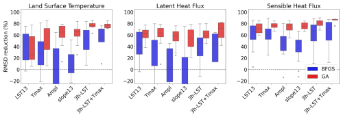
Figure 2 Box plots obtained within 16 optimization tests with random first-guess parameter values for each DA experiment over the selected site in Spain (ES-Abr) comparing the performance between the gradient-based (in blue) and genetic (in red) methods in terms of the model–data RMSD reduction (%) obtained for 30 min LST, LE, and H. The x axis indicates the DA experiment assimilating a single characteristic of the diurnal cycle (LST13, T_max, Ampl, and slope13), the 3 h LST pseudo-observations (LST), and with the addition of T_max (LST + T_max). The RMSD reduction (%) is computed between the 16 posterior simulations per DA experiment and the prior simulations (generated from a single set of prior parameters).

Overall, it becomes evident that the BFGS method is more reliant on initial first guesses, shown by the larger spread in each DA experiment for the three analysed variables (LST, LE, and H). This confirms the higher likelihood of gradient-based methods getting stuck in local minima. Notably, the GA method consistently outperforms the BFGS method, yielding more substantial improvements, with the RMSD reduction surpassing that achieved by BFGS in every experiment and for each variable. Remarkably, the GA method shows improvements across all three variables, and each of the 16 runs achieves RMSD reductions greater than 0. Conversely, certain optimizations employing the BFGS method result in deteriorated simulations after the assimilation, with a negative RMSD reduction for the 30 min LST and LE. This is obtained mainly when the amplitude (Ampl) and morning slope (slope13) of the LST diurnal cycle are assimilated. This underscores the superior reliability and performance consistency of the GA method compared with the BFGS method across the evaluated variables and experiments.

Concerning the improvements in 30 min LST simulations through various DA experiments, superior performance is observed when assimilating the full LST series alone or incorporating a characteristic of the diurnal cycle in the assimilation (utilizing T_min, T_max, and/or Ampl; see Fig. S1 in the Supplement). Nevertheless, incorporating T_min, T_max, and/or Ampl into the full LST series results in only marginal additional improvement in 30 min LST simulations. In fact, the median reductions in the RMSD remain consistently similar, around 76 %–79 %, across all experiments using the full LST series as a constraint. In contrast, the assimilation of a single LST observation per day – such as LST at 13:00 LT (LST13) or maximum daily LST (T_max) only – leads to significantly less improvement in the 30 min LST simulation. Median reductions in the RMSD are 26 % for LST13 and 45 % for T_max, accompanied by notably larger spreads, similar to those obtained with the BFGS method.

Regarding the improvements in the 30 min simulations of the surface turbulent fluxes (LE and H), the results are much more stable than those obtained for LST across the different DA experiments. This stability is observed in terms of reductions in the RMSD (median and distributions) across the 16 independent runs. While the median reductions in the RMSD of LE range between 55 % and 72 % for the slope13 and 3 h-LST + T_max experiments, respectively, the improvements in H range between 71 % and 87 % for the LST13 and 3 h-LST + T_max experiments, respectively. It should be noted that jointly assimilating T_max and LST (3 h-LST + T_max) considerably improves the LE and H simulations compared with assimilating LST only, with a 59 % and 81 % RMSD reduction for LE and H, respectively. The 3 h-LST + T_max experiment not only offers superior performance with respect to simulating H but also produces the least dispersion in RMSD reduction. As can be seen, larger improvements using the GA method are obtained in H simulations, with a higher RMSD reduction and smaller spreads than those depicted for LST and LE, as can be noticed from the interquartile ranges.

Summarizing the results focusing only on those from GA and the three analysed variables, the most substantial enhancements are found when considering the entire 3 h LST series, either independently (3 h-LST DA experiment) or jointly with other attributes of the diurnal cycle such as the 3 h-LST + T_max DA (or the 3 h-LST + Ampl and 3 h-LST + Ampl + T_max experiments; not shown). These configurations yield an average RMSD reduction of between 72 % and 78 % for the three variables (LST, LE, and H). Conversely, assimilating a single characteristic of the diurnal cycle (the LST13, T_min, T_max, Ampl, slope13, and slope19 DA experiments) results in comparatively smaller improvements, with an average RMSD reduction of between 53 % and 67 %. Furthermore, it is worth noting that assimilating a single daytime observation independently of all other observations throughout the day, specifically to calculate diurnal cycle characteristics (e.g. LST at 13:00 LT), yields the least improvement in LST posterior simulations. When considering the potential assimilation of data from upcoming thermal missions like TRISHNA or LSTM (Land Surface Temperature Monitoring), which will provide LST at 13:00 LT to primarily detect water stress (Lagouarde et al., 2019; Koetz et al., 2018), our findings suggest that assimilating LST13 in ORCHIDEE is less optimal to enhance the diurnal cycle of LST and energy fluxes, compared with other constraints. It is interesting to compare the performance obtained by assimilating a single LST at 13:00 LT (LST13) with the daily maximum LST (T_max), which typically occurs at 16:00 LT on a 3 h basis at the ES-Abr site. The LST13 experiment results in lower improvements with respect to LST and H simulations than when assimilating T_max. Specifically, the median RMSD reductions in LST simulations are 26 % for the T_max experiment and 45 % for the LST13 experiment. Conversely, both experiments (T_max and LST13) yield nearly identical median RMSD reductions (63 % and 64 %, respectively) in LE simulations, slightly higher than assimilating the entire 3 h LST time series (59 %). In any case, the fact that the errors in the surface fluxes and LST simulations have been reduced by assimilating a single observation at 13:00 LT confirms the potential use of TRISHNA or LSTM for monitoring water resources.

Nevertheless, through the combination of different characteristics of the diurnal cycle, such as in the LST13 + slope13 + slope19 and Ampl + LST13 + slope13 + slope19 DA experiments (not shown), noteworthy improvements similar to those achieved using the entire LST series can be attained, with an average RMSD reduction of 74 % for both experiments.

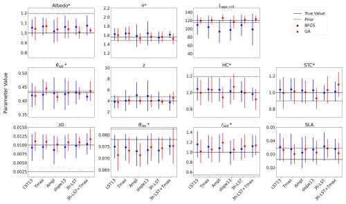
Figure 3 Parameter estimates for each DA experiment over the selected site in Spain (ES-Abr) comparing the 11 optimized parameters between the gradient-based (in blue) and genetic (in red) methods. Parameter estimates are represented by the mean and standard deviation across 16 optimization tests with random first-guess parameter values. The x axis indicates the DA experiment assimilating a single characteristic of the diurnal cycle (LST13, T_max, Ampl, and slope13), the 3 h LST pseudo-observations (LST), and including the T_max (LST + T_max). The true parameter (default ORCHIDEE value) and prior values (defined randomly) are represented by the solid and dashed horizontal lines, respectively.

3.1.2 Parameter and uncertainty estimates

The optimized parameters from the different DA experiments are illustrated in Fig. 3. In general, when utilizing the GA method, the averages of the optimized parameters from the 16 independent runs per DA experiment closely align with the true parameter values for a majority of the parameters. This holds especially for n, L_age,crit, and z, which are among the most LST-sensitive parameters according to the sensitivity analysis (see Fig. B1). Furthermore, irrespective of the DA experiment, these three parameters exhibit the smallest standard deviation. This indicates that the GA method consistently converges accurately to the true parameter values across the 16 runs. It is worth noting that the most sensitive parameter (Albedo^*) does not show stable results across DA experiments using the GA method. While Albedo* shows mean values in close proximity to the true value, it exhibits larger spreads when assimilating single characteristics of the diurnal cycle, such as those observed with the BFGS method. This behaviour can be attributed to the nature of this surface albedo parameter, which was defined as a multiplicative factor applied to two albedo components associated with vegetation and soil. This configuration may lead to error compensation effects between several parameters when assimilating a single characteristic, preventing a unique solution for Albedo^* in the optimization process. Nevertheless, when assimilating a combination of four or five characteristics of the diurnal cycle, such as the Ampl + LST13 + slope13 + slope19 and Ampl + T_max + LST13 + slope13 + slope19 DA experiments (see Fig. S2), the obtained results are comparable to assimilating the 3 h LST alone. In these cases, the mean optimized values are very close to the true value, and the spreads are smaller, indicating a more accurate and consistent assimilation outcome.

Even though HC^* (related to soil heat capacity) and STC^* (related to soil thermal conductivity) are among the most sensitive parameters to the selected characteristics of the diurnal cycle (Fig. B1), their retrieval is not optimal for all DA experiments, as indicated by large spreads in their optimized values. This is directly linked to the fact that they are highly anticorrelated with other parameters, as evidenced by the posterior covariance matrix (see Fig. S3).

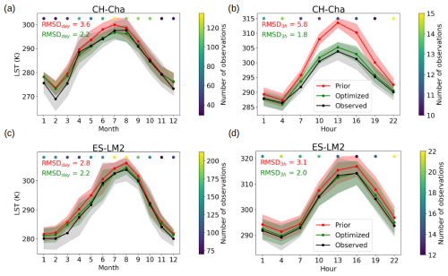
Figure 4 Annual cycle (a, c) and diurnal cycle in June (b, d) of LST for 2018 over a grassland (CH-Cha; a, b) and a cropland (ES-LM2; c, d) site. Observed LST represents the mean (black dot) and standard deviation (shaded area) of 3 h CCI-LST data. The mean and standard deviation of Prior and Optimized LST are computed from the same CCI-LST availability. Coloured dots at the top of each plot represent the number of CCI-LST observations per month or hour. The RMSD on a daily (RMSD_day; a, c) and 30 min (RMSD_3 h; b, d) basis is shown for Prior (red) and Optimized (green) simulations. Note that the 30 min LST is evaluated at 3 h intervals when CCI-LST is available.

In our efforts to evaluate the potential of assimilating the CCI-LST product to constrain ORCHIDEE parameters using twin experiments, we also consider the actual availability and uncertainties associated with CCI-LST over the pixel corresponding to the ES-Abr site (Appendix C). We conduct two DA experiments with the GA method: assimilating the 3 h LST series alone (3 h-LST DA) and incorporating the T_max (3 h-LST + T_max DA). For both DA experiments, the RMSD values are comparable to those obtained when considering the full pseudo-data series, although lower, particularly for LE (Fig. C1). However, the availability of CCI-LST data may significantly impact the estimation of daily maximum LST (T_max) – as well as the other characteristics – especially at sites characterized by climates with higher cloud occurrence compared with the ES-Abr site. Consequently, when conducting the real DA experiments, we only consider the entire 3 h CCI-LST series (LST DA).

3.2 DA based on actual LST observations

From the above twin experiments, we concluded that the optimal DA set-up to be used with the CCI-LST product is the assimilation of the 3 h CCI-LST data with the GA method. Thus, we run such an optimization for the year 2018 across the 34 Warm Winter sites. Figure 4 illustrates the annual and diurnal cycles of LST in June at two contrasting sites: Chamau in Switzerland (CH-Cha; Fig. 4a, b), characterized by a humid and cool temperate climate (Cfb, according to Köppen–Geiger), and Las Majadas South in Spain (ES-LM2; Fig. 4c, d), characterized by a dry Mediterranean climate (Csa). LST simulations using default ORCHIDEE parameters (Prior) and optimized parameters after assimilating CCI-LST data (Optimized) are compared against in situ fluxes. At both sites, the Prior LST simulations are clearly overestimated with respect to both the annual and diurnal cycles. The Optimized LST is improved at both sites, with the RMSD being decreased from 3.6 to 2.2 K at CH-Cha and from 2.8 to 2.2 K at ES-LM2 on a daily basis. The improvement is more noticeable at an hourly timescale during daytime hours in June (Fig. 4b, d), particularly at the CH-Cha site, where the assimilation of CCI-LST data significantly corrects the Prior overestimation. At the CH-Cha site, the RMSD is decreased from 5.2 to 1.8 K, while the RMSD is decreased from 3.1 to 2.0 K at ES-LM2. Although the bias in Prior LST on a monthly scale is substantially corrected, the assimilation process encounters difficulties in fully addressing the overestimation observed in winter months (Fig. 4a, b, c). The latter is mainly attributed to a reduced availability of data during colder months. It is noteworthy that the number of observations in winter months can be nearly a third of that in summer, contributing to the difficulties observed. In addition, the issue is also influenced and inherently connected to a weakened constraint of LST on the surface energy balance under radiation-limited conditions.

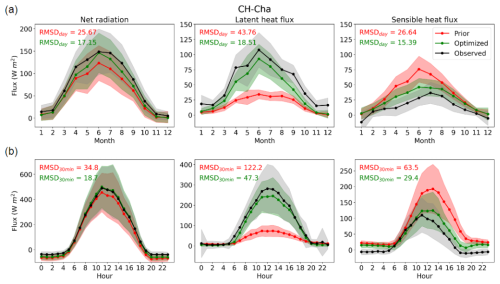
Figure 5 Annual cycle (a) and diurnal cycle in June (b) of R_n (left panels), LE (middle panels), and H (right panels) for 2018 over a grassland (CH-Cha) site. The mean (dot) and standard deviation (shaded area) are represented for in situ observations (black) and for Prior (red) and Optimized (green) ORCHIDEE simulations. The RMSD on a daily (RMSD_day; a) and 30 min (RMSD_30 min; b) basis is shown for Prior (red) and Optimized (green) simulations.

Figures 5 and 6 illustrate the annual and diurnal (in June) cycles of Prior and Optimized R_n, LE, and H compared against in situ observations at the same contrasting sites (CH-Cha and ES-LM2). At both sites, Prior R_n and LE are underestimated, whereas Prior H is overestimated, which is linked to the overestimated Prior LST shown in Fig. 4. Similarly to the improvements observed in LST simulations, the assimilation of CCI-LST data effectively corrects much of the underestimation in R_n and LE at both monthly (Fig. 4a, c) and hourly (Fig. 4b, d) scales. Notably, improvements are evidenced during summer months and daylight hours (between 08:00 and 18:00 UTC). At both sites, the LE fluxes exhibit more pronounced improvements compared with R_n and H, in contrast to the twin DA experiments where the improvement is more important for H. At the CH-Cha site (Fig. 5), the RMSD values in LE fluxes are reduced from 43.8 to 18.5 W m⁻² and from 122.2 to 47.3 W m⁻² on a daily and 30 min basis, respectively, both representing an improvement of about 60 %. At the ES-LM2 site (Fig. 6), the RMSD values are reduced from 20.1 to 8.8 W m⁻² and from 62.2 to 35.3 W m⁻² on a daily and 30 min basis, respectively. Regarding H, significant enhancements are observed at CH-Cha, whereas improvements at ES-LM2 are slight and mostly noticeable from March to May and during night-time hours (between 19:00 and 06:00 UTC). In fact, the RMSD in 30 min H at CH-Cha is decreased from 63.5 to 29.4 W m⁻², while it is slightly increased from 60.3 to 63.5 W m⁻² at ES-LM2. The disparity in improvements between the two sites can be attributed to the complexity of surface heterogeneity. Additionally, soil heat fluxes and water infiltration capacity, both presenting significant uncertainties in modelling and measurement, become particularly crucial at semi-arid sites. For instance, at the ES-LM2 site, H is significantly overestimated during daytime hours in summer, indicating that the soil heat flux is correspondingly underestimated. CH-Cha, characterized as a homogeneous grassland site and well-classified in ORCHIDEE's PFT maps, experiences a significant improvement in all three surface energy fluxes. Conversely, at ES-LM2, a more complex savanna site predominantly covered by Quercus ilex and grass but classified as cropland when used in ORCHIDEE, shows a comparatively smaller improvement, particularly in terms of H.

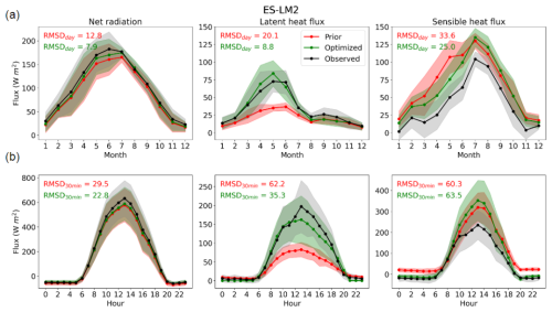
Figure 6 Annual cycle (a) and diurnal cycle in June (b) of R_n (left panels), LE (middle panels), and H (right panels) for 2018 over a cropland site (ES-LM2). The mean (dot) and standard deviation (shaded area) are represented for in situ observations (black) and for Prior (red) and Optimized (green) ORCHIDEE simulations. The RMSD on a daily (RMSD_day; a) and 30 min (RMSD_30 min; b) basis is shown for Prior (red) and Optimized (green) simulations.

Figure 7 illustrates the performance of assimilating 3 h CCI-LST data for the year 2018 across the 34 sites, showcasing the RMSD reduction in LST, R_n, LE, and H. Throughout all of the sites, the assimilation of CCI-LST data leads to improvements in LST simulations. The enhancements in LST reach up to a 60 % RMSD reduction from Prior to Optimized simulations, with a median value of 24.6 % across all sites. Furthermore, at the majority of the sites, the assimilation also yields improvements in the three energy fluxes. Specifically, R_n, LE, and H exhibit RMSD reduction improvements at 72.0 %, 79.4 %, and 70.6 % of the sites, respectively. Remarkably, the most substantial enhancements are observed in LE, with an RMSD reduction of up to 60 % and median values of 19.9 %, followed by R_n and H, both with medians of 9.5 %.

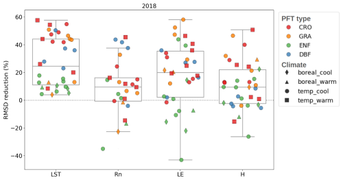
Figure 7 Box plots showing the performance, in terms of model–data RMSD reduction (%), obtained for hourly R_n, LE, and H over sites assimilating 3 h LST from the ESA CCI product in 2018. Note that, in 2018, R_n is only available for 25 of the 34 sites assessed.

We observe that superior performance with respect to LST and turbulent fluxes (LE and H) is achieved at grassland and cropland sites, whereas the worst results are observed at evergreen needleleaf forest (ENF) sites. Particularly noteworthy are the substantial improvements in LE for grassland sites, with a median RMSD reduction for each PFT of between 21 % and 47 %. Meanwhile, H improvements in grasslands and croplands are about 20 %. In contrast, the assimilation outcomes for forest sites do not demonstrate comparable success. It is important to highlight that the four ENF sites with cool boreal climates show degradation in fluxes after assimilation, with the exception of the CH-Aws site. This deterioration is linked to the complex terrain of these four sites, which are situated in mountainous regions with a cool boreal climate, including three in the Alps (CH-Aws, CH-Dav, and IT-Ren) and one in the Carpathians (CZ-BK1). On the other hand, ENF in other climates demonstrates varied performance across sites, with no overall change in the RMSD for LE (median RMSD reduction of 0.9 %). However, there is an improvement in terms of the RMSD reduction for H, approximately 9.3 %. That can be explained by the fact that evapotranspiration in these forests is less affected by water stress, as their roots can extract water deeper, and therefore the vegetation temperature is more stable and does not contribute much to the optimization of LE.

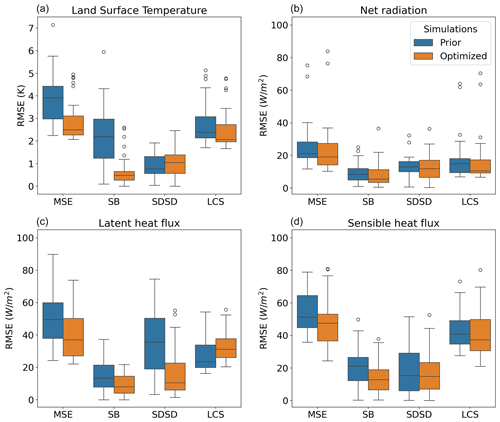
Figure 8 Box plots showing the decomposition of the mean-square error (MSE) in terms of bias (SB), difference in the standard deviations (SDSD), and lack of correlation (LCS) between the model and observations for 30 min LST (a), R_n (b), LE (c), and H (d) across sites in 2018. For clarity, note that the square root of the error components is plotted.

Figure 8 depicts the breakdown of the MSE into the bias (SB), difference in the standard deviations (SDSD), and lack of correlation (LCS) across sites for LST and the three simulated fluxes using the default ORCHIDEE parameters (Prior) and the optimized parameters after assimilating CCI-LST data (Optimized). The MSE in LST is significantly decreased from the Prior to Optimized ORCHIDEE simulations in terms of both the median and spread values. In practice, the median MSE decreases from 3.91 to 2.50 K, representing an MSE reduction of 36 % from Prior to Optimized LST in the model–data fit. This MSE reduction comes mainly from the reduction in the two major components of the Prior MSE: SB and LCS. The bias component (SB) shows an important improvement that is decreased from 2.20 to 0.49 K (i.e. decreased by 78 %) from the Prior to Optimized simulations. Although the SDSD component shows a degradation (increased) after assimilation, this error remains small (i.e. with median values of 0.77 to 1.06 K). This degradation is explained by a slight underestimation of the standard deviation of simulations compared with that of observations, which are the first and second terms of Eq. (5), respectively. Consequently, this leads to an augmentation in the disparity between the standard deviations of simulations and observations.

Figure 9 Box plots showing the decomposition of the MSE per season in terms of bias (SB), difference in the standard deviations (SDSD), and lack of correlation (LCS) between the model and observations for 30 min LST across sites in 2018. For clarity, note that the square root of the error components is plotted.

The MSE components in R_n show similar and relatively smaller values, ranging between 0 and 40 W m⁻², whereas they can exceed 80 W m⁻² in LE and H. After assimilation, significant improvements are evident across all three components (SB, SDSD, and LCS), as observed in the medians of the Optimized simulations. With the exception of LCS in LE, the medians are significantly reduced for the three fluxes, reflecting a substantial reduction in the MSE components after assimilating CCI-LST data. For LE, the ORCHIDEE model using default parameters (Prior) mainly struggles with respect to simulating the amplitude of the seasonal cycle across a majority of sites, as evidenced by the substantial Prior SDSD with a high median (35.5 W m⁻²) and significant spread. The SDSD is significantly reduced by 70 % after assimilating LST data, along with a 40 % reduction in the bias component (SB). However, the fluctuation pattern is compromised, as indicated by a larger LCS for Optimized simulations, signifying a 33 % deterioration in the temporal pattern. Regarding H, all three components show improvement, with particular enhancements in the bias (SB) (which is reduced by 40 %), as for LE. Even though the temporal pattern (LCS) of H is reduced by 9 %, it remains the most important component for a majority of sites, as seen by a large median and spread in Optimized H. This can also be observed in the MSE decomposition by site (illustrated in Fig. D1). Therefore, the assimilation faces challenges primarily with respect to enhancing the temporal pattern of turbulent fluxes, where LCS is the major MSE component in LST, LE, and H, constituting 47 %, 71 %, and 61 % of the total MSE, respectively.

The challenge related to the temporal pattern of turbulent fluxes, represented by the lack of correlation component, is further highlighted when examining the correlation coefficient between simulations and observations, analysed separately for each hour and month (not shown). During daytime hours (between 08:00 and 16:00 UTC), median correlations are equal to 0.81 for both LE and H. However, during night-time hours (between 20:00 and 04:00 UTC), these correlations drop to 0.15 for LE and to 0.46 for H, as could be expected given the much lower values of the fluxes encountered during night-time. While the disparity is less pronounced on a monthly scale, median correlations in December and January are notably lower (0.41–0.46 for LE and 0.53 for H) compared with the rest of the year. The median correlation values range between 0.64 (in November) and 0.90 (May–June) for LE and between 0.75 (November) and 0.92 (August) for H.

Figure 9 shows the breakdown of the MSE in LST per season, highlighting the periods when the assimilation of CCI-LST data exerts a more pronounced impact throughout the year. Similar to the overall MSE in LST shown in Fig. 8, the MSE in spring (April–May–June, AMJ, in Fig. 9) and summer (July–August–September, JAS) experiences a substantial reduction in terms of the median value, from 4.2 to 2.3 K and from 3.7 to 2.3 K, respectively. Conversely, the MSE values in winter (January–February–March, JFM) and autumn (October–November–December, OND) are slightly reduced, from 3.0 to 2.8 K, for both seasons. In all seasons, the bias component is the most reduced component after assimilating the 3 h CCI-LST. For instance, during warmer seasons (AMJ and JAS), the bias component experiences the most significant reduction, with median values decreasing by 72 % (from 3.0 to 0.8 K) and 86 % (from 2.2 to 0.3 K) in AMJ and JAS, respectively. In addition, the spread of the bias component is markedly diminished during these seasons. However, in both seasons, the difference in standard deviations (SDSD) increases, indicating that the assimilation of CCI-LST data encounters challenges with respect to improving the amplitude of the seasonal cycle, which is consistent with observations for the rest of the year. As discussed above, the smallest improvements in LST simulations in colder seasons can mainly be linked to the reduced availability of data (more cloudy conditions) during colder months, as observed in Fig. 4 for two contrasting sites. It is worth noting that the availability of data in winter is, on average, 63 (±30) observations per month across all sites, whereas the average is increased to 118 (±35) observations per month in summer.

As observed in the case of LST (and closely associated with it), similar seasonal enhancements are evidenced for the surface energy fluxes (R_n, LE, and H), indicating further improvements during warmer seasons (see Fig. S4). During spring (AMJ) and summer (JAS), significant reductions in the MSE are observed for all three fluxes after optimization, particularly for LE, where the MSE is reduced by 28 % and 22 % for AMJ and JAS, respectively. Notably, during these seasons (AMJ and JAS), LE presents significant improvement in both the bias and SDSD components. Similarly, the bias component is significantly improved for H after assimilating CCI-LST data. However, the three fluxes exhibit slight enhancements in the MSE during winter (JFM) and autumn (OND), with median values of their components being quite comparable between Prior and Optimized simulations. Confirming the evidence presented in Fig. 8 across all variables assessed (LST and fluxes) during 2018, the lack of correlation component (LCS) in Optimized simulations emerges as the primary MSE component for all seasons, exhibiting the least improvement following the assimilation of CCI-LST data. Consequently, the LCS remains the dominant MSE component for all variables and seasons, with the exception of R_n in spring (see Fig. S4).

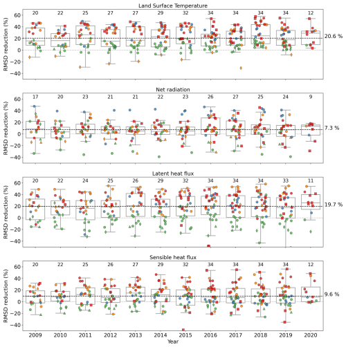
Figure 10 Box plots showing the performance, in terms of model–data RMSD reduction (%), obtained for 30 min LST, R_n, LE, and H from 2009 to 2020 using optimized parameters per site in 2018. The number of sites with available data per year is shown above each box plot. The dashed black line represents the average of the medians over the years. The colour represents the dominant vegetation type per site: CRO (cropland) – red; GRA (grassland) – orange; DBF (deciduous broadleaf forest) – blue; and ENF (evergreen needleleaf forest) – green. The symbols represent the climate: warm temperate – squares; cool temperate – circles; warm boreal – triangles; and cool boreal – diamond.

3.2.1 Model performance for the evaluation period

The parameters optimized from the assimilation of CCI-LST data in 2018 over each site are used to simulate LST and surface energy fluxes during the evaluation period (2009–2020) for stations with available in situ data. Figure 10 shows the performance with respect to the RMSD reduction in LST, R_n, LE, and H considering optimized parameters across the 34 sites from 2009 to 2020. In contrast to the optimization year (2018), some deterioration is observed in LST for a couple of sites during the validation period. The results obtained for the three fluxes for each year are very similar to those obtained in the optimization year, with most of the sites presenting improvements using the optimized parameters in 2018. In fact, the median RMSD reduction values per year are quite stable across years for the three fluxes, which are equal to 7.2 %, 19.7 %, and 9.5 % for R_n, LE, and H, respectively. As found in 2018 for LE and H, better performance is observed for grassland and cropland sites, whereas the worst performance is found in ENF and boreal climates when compared with the other vegetation and climate types. Specifically, the ENF sites systematically exhibit less improvement or even deterioration for LST and LE, with RMSD reductions falling below their median values.

3.2.2 Improvement in fluxes from average parameters

We calculate the median of optimized parameters across sites to account for a unique set of PFT-specific parameters. Thus, we run ORCHIDEE with this unique parameter set for each PFT over the 34 sites from 2009 to 2020 to evaluate the effectiveness of optimized parameters at larger scales. This assessment aims to determine whether the improved performance at each site aligns with that achieved using site-specific parameters.

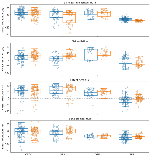
Figure 11 Box plots showing the performance, in terms of model–data RMSD reduction (%), obtained for 30 min LST, R_n, LE, and H across all sites from 2009 to 2020 using optimized parameters per site (blue) and a single set of parameters per PFT (orange). The site-specific parameters are obtained from the assimilation of 3 h CCI-LST observations in 2018, whereas the PFT-specific parameters are obtained from the median of these site-specific parameters per vegetation type.

Although the performance over the years is inferior for LST compared with that obtained using optimized parameters for each site, the results obtained for the three fluxes remain quite similar (see Fig. 11). The averaged median RMSD reduction across years for LST decreases to 13.8 % using PFT-specific parameters, instead of 20.6 % using the parameters optimized for each site. In turn, the median RMSD reduction values per year for the three fluxes exhibit not only consistent stability across the years, comparable to using site-specific parameters (Fig. 10), but also a slight increase. The average medians for R_n, LE, and H are notably higher, reaching 13.1 %, 20.7 %, and 9.6 %, respectively, compared with average medians of 7.3 %, 19.7 %, and 9.6 % using site-specific parameters. It is noteworthy that R_n experiences additional improvement when utilizing a unique set of parameters. This enhanced improvement is mainly visible at grassland and cropland sites, which show more significant improvement when using a unique set of parameters, as illustrated in Fig. 11. Particularly remarkable are the substantial enhancements at grassland sites, with all sites experiencing an improvement in R_n simulations using PFT-specific parameters compared with site-specific parameters. In fact, the median RMSD reduction in R_n simulations is increased from 4 % using site-specific parameters to 17 % using PFT-specific parameters. These improvements are particularly observed at sites characterized by boreal climates, where the assimilation of CCI-LST data struggles to enhance simulations. However, certain sites experience a decline when employing a unique set of parameters, notably the ENF sites. The LST and R_n simulations over these sites deteriorate in comparison to both prior simulations and those utilizing site-specific optimized parameters.

In contrast, improvements in RMSD reductions for LE and H using a unique set of optimized parameters are comparable (or even superior) to using site-specific optimized parameters across the four vegetation types. Notably, grassland sites exhibit significant additional enhancements for LE and H when employing a unique set of parameters, with the exception of sites under temperate cool climates for LE.

While multi-site optimization using only LE and H data has been proven to further enhance model performance compared with averaging site-specific parameter values (Kuppel et al., 2012), its implementation can become challenging with LST data, given that we have numerous PFTs and soil textures, resulting in a multitude of cases to consider. Our findings suggest that using the median of site-specific parameters can offer a practical and effective alternative to calibration, particularly in cases where a multi-site set-up would be overly complex.

4 Discussion

According to our results, we expect that using the PFT-specific parameters derived from the 34 evaluated sites will enhance ORCHIDEE simulations of LST and energy fluxes at a regional scale. While improvements are anticipated for croplands, grasslands, and deciduous broadleaf forests, they are less likely for evergreen needleleaf forests, especially in boreal climates. It is important to note that, in this study, only 7 of the 15 ORCHIDEE PFTs are represented by these sites, with some, like boreal evergreen needleleaf forests, being underrepresented. This study seeks to improve simulations of LST and surface energy fluxes at a regional scale. However, ongoing work aims to assimilate CCI-LST data across various pixels for all PFTs, ensuring identical representation (i.e. the same number of pixels per PFT).

4.1 Impact of the optimization period

We acknowledge that the selection of a particular year for optimization may impact the selection of parameters to optimize and the performance of the assimilation. Regarding the selection of parameters for optimization, we conducted two sensitivity analyses at the 34 sites for both 2017 and 2018, separately. The selected parameters for optimization were generally consistent between the 2 years, with the exception of the parameters controlling the water stress curve (α) and the critical soil moisture above which transpiration is maximal (θ_crit,rel). In 2017, α and θ_crit,rel were selected for optimization at 7 and 6 sites, respectively, whereas both parameters were selected at 13 sites in 2018. This difference is attributed to the drought conditions in 2018, which increased the relevance of these water-stress-related parameters. Properly representing these parameters is crucial for future projections of climate and water resources (Fu et al., 2022, 2024), highlighting the importance of considering the appropriate conditions for accurately optimizing the processes that we aim to improve.

In the twin experiments at the ES-Abr site, we assessed the impact of selecting a specific year (2018) versus the entire available 6-year period (2015–2020) on the performance of 30 min LST and turbulent fluxes during 2017 (see Fig. E1). We chose 2017 to ensure a more independent evaluation of both calibration periods (2018 and 2015–2020). The results showed no significant differences with respect to improving the fluxes in 2017 between using the entire period (2015–2020) and a single year (2018) for calibration. Although using the entire period resulted in a slightly higher RMSD reduction for the three variables with the GA method, the BFGS method yielded superior performance when using only 2018 for calibration. This may seem counterintuitive, as additional information typically creates extra constraints, helping to smooth the cost function and making local minima less likely for BFGS. However, our findings can be explained by the fact that drought periods in 2018 are less predominant in a 6-year period, resulting in a less optimal solution for the calibration of the water stress parameters with the BFGS method.

4.2 Impact on vegetation phenology and soil water

We recognize that assimilating LST alone has its limitations and cannot enhance the model–data fit of all variables controlling water, energy, and carbon fluxes. To better understand the performance of the LST assimilation procedure on other variables less directly linked to energy fluxes, we assessed the impact of LST optimization on soil water availability and gross primary productivity (GPP). As the number of sites with available soil moisture data are limited and measurement depths vary among sites, we evaluated the impact on the top 10 cm of soil moisture in our twin experiments. The soil moisture showed a clear improvement (positive median RMSD reduction) when assimilating the 3 h LST alone using the GA method. The median RMSD reduction for this experiment (3 h-LST) represented a 10.4 % enhancement in the soil moisture, although some runs among the 16 different first guesses resulted in a deterioration of soil moisture. The fact that the 3 h-LST DA showed an overall improvement in soil moisture confirms the chosen strategy for the assimilation of the CCI-LST data.

Regarding the GPP, we assess the impact by assimilating the 3 h CCI-LST time series over the 34 Warm Winter sites in 2018. Assimilating the 3 h LST data results in an overall degradation in GPP, with a median RMSD increase of 7.4 % across sites. Among the studied sites, 14 of 34 show improvements under diverse conditions, such as the grassland CH-Cha and Mediterranean ES-LS2 sites (see Fig. F1). At the other sites, larger errors were obtained, with RMSD increases of up to 55.4 %. For instance, while the cropland CH-Oe2 site exhibits a 36.1 % improvement in LE, the RMSD in GPP is increased by 41.3 % (see Fig. F2). Despite the mixed results obtained for GPP, the improvement observed at the 14 sites (i.e. 41 % of the sites) is a promising outcome, especially considering the challenge with respect to enhancing model variables that are not closely linked to LST. In fact, assimilating a single data stream may even degrade the model simulations of other variables, as shown in Kato et al. (2013) and Bacour et al. (2015, 2023). In our study, as we calibrated only parameters impacting LST and kept the carbon-related parameters previously optimized without LST observations, a degradation of the carbon fluxes is not surprising. Nonetheless, the overall improvement in the energy fluxes, such as the 20.6 % enhancement in LE and 9.6 % enhancement in H, is significantly more impactful than the observed degradation in GPP.

Although improvements in soil moisture and phenology were not expected when assimilating only LST data, the enhancements found in the twin experiments for soil moisture and at some sites for GPP (in the DA experiments based on actual data) are very encouraging. These results support ongoing efforts to jointly assimilate LST with satellite-derived products such as the leaf area index, albedo, or soil moisture into ORCHIDEE. Such an approach is expected to better constrain a wider range of energy, water, and carbon parameters, enhancing the overall performance of the model.

5 Summary and conclusions

This study focuses on the assimilation of ESA CCI-LST data into the ORCHIDEE land surface model with the aim of refining LST and surface energy flux simulations. Through a series of synthetic twin DA experiments, we explore different optimization methods (BFGS and GA) and assimilated state variables (individual LST observations and characteristics of the LST diurnal cycle) to determine the most effective assimilation strategy. The selected strategy is then implemented to assimilate actual CCI-LST data across 34 European sites in an optimization year (2018) and, finally, validated from 2009 to 2020.

The results from the twin DA experiments reveal that the genetic algorithm (GA) consistently outperforms the BFGS method, evidencing more substantial improvements than those achieved by BFGS in all DA experiments for both LST and turbulent fluxes. This superiority is underscored by the reliability and consistency exhibited by the GA method. This is exhibited not only in RMSD reductions from prior to posterior simulations but also in the consistent convergence to the true parameter values across the 16 runs with random first guesses, particularly for the most LST-sensitive parameters.

Concerning the performance of the model optimization, our findings show that the most substantial enhancements are evidenced when considering the entire 3 h LST series, either individually (the LST DA experiment) or jointly with other attributes of the diurnal cycle (the LST + T_max, LST + Ampl, and LST + Ampl + T_max DA experiments). In contrast, assimilating a single characteristic of the LST diurnal cycle (e.g. LST at 13 h, daily minimum, maximum, amplitude, and morning and afternoon gradients) yields comparatively smaller improvements in both the LST and H simulations. Conversely, for LE, assimilating a single characteristic such as LST13, T_max, T_min, or Ampl, resulted in an improvement very close to that obtained by the entire 3 h LST series. Our findings suggest that assimilating LST at 13:00 LT, as will be possible with the forthcoming TRISHNA and LSTM missions, can significantly enhance LE simulations. This highlights the valuable contribution that these missions can make to the future modelling of the Earth's surface and monitoring of water resources. Nevertheless, through the combination of different characteristics of the diurnal cycle, noteworthy improvements similar to those achieved using the entire 3 h LST series can be reached for both LST and turbulent fluxes. It should be noted that these outcomes are obtained considering the full availability of 3 h pseudo-observations, so they might be considerably degraded with the actual availability of CCI-LST (i.e. considering cloudy conditions).

Therefore, we proceed with the assimilation of actual CCI-LST data over 34 European sites, focusing exclusively on the complete 3 h CCI-LST series (LST DA). The limitation stems from the scarcity of available LST observations per day, especially at sites situated in boreal climates that are more prone to the occurrence of cloudy conditions. Consequently, this specific DA experiment is identified as the most effective assimilation strategy, as introducing additional characteristics to the LST series does not yield a substantial further advantage in the assimilation process.

The optimization of key parameters for each site leads to a remarkable enhancement in the surface energy fluxes at the in situ level, with improvements observed across LST, R_n, LE, and H. Notably, the optimization conducted over a single year yields improved ORCHIDEE simulations over the entire 11-year validation period. The benefits of this optimization are not uniform and vary depending on vegetation types and climates. For instance, cropland and grassland sites exhibit larger reductions in the RMSD compared with forested sites, particularly for evergreen needleleaf forests, where degraded simulations are observed after assimilation. Similarly, warmer climates show a greater RMSD reduction than boreal climates, where the assimilation of LST struggles to enhance LST and energy fluxes. The latter is explained by the fact that water is not limiting at evergreen needleleaf forest sites or in cold climates, leading to a weakened LST–evapotranspiration relationship (i.e. energy-limited evapotranspiration regimes).

To evaluate the applicability and effectiveness of optimized parameters at a broader scale, from regional to global scales, we employ a unique set of parameters for each PFT obtained from the optimization for each site. We evaluate ORCHIDEE simulations using the median of parameters specific to vegetation type (PFT-specific) across all 34 sites from 2009 to 2020. Significantly, the performance for both LST and fluxes exhibits not only consistent stability over the years, comparable to using site-specific parameters, but also indicates a slight improvement in energy fluxes. However, assimilating LST alone has limitations and cannot improve all variables controlling water, energy, and carbon fluxes. Nevertheless, our findings reveal promising outcomes, such as the clear improvement in soil moisture in the twin experiment and the enhancement of GPP at several studied sites. Despite the challenges, these results indicate that LST data can positively influence variables less directly linked to energy fluxes. This underscores the potential of combining LST with other satellite-derived products, such as the leaf area index, albedo, and soil moisture, to better constrain and improve the overall performance of the ORCHIDEE model.

Furthermore, our findings underscore the notable impact of the ESA CCI-LST product and its associated uncertainty on effectively constraining water and energy fluxes within the ORCHIDEE model. This suggests that integrating CCI-LST data can substantially contribute to further improving climate simulations with Earth system models and advancing our comprehension of land–atmosphere interactions. However, future research is essential to refine the utilization of uncertainties provided by the CCI-LST product. This involves integrating time-varying observation errors derived from the 3 h LST uncertainty associated with each observation into ORCHIDAS as well as exploiting the decomposed uncertainties while considering their spatio-temporal variability.

Appendix A: Sites and pseudo-observations assimilated

Table A1 Main characteristics of sites used in this study in terms of location, availability of data (years), and vegetation and climate types.

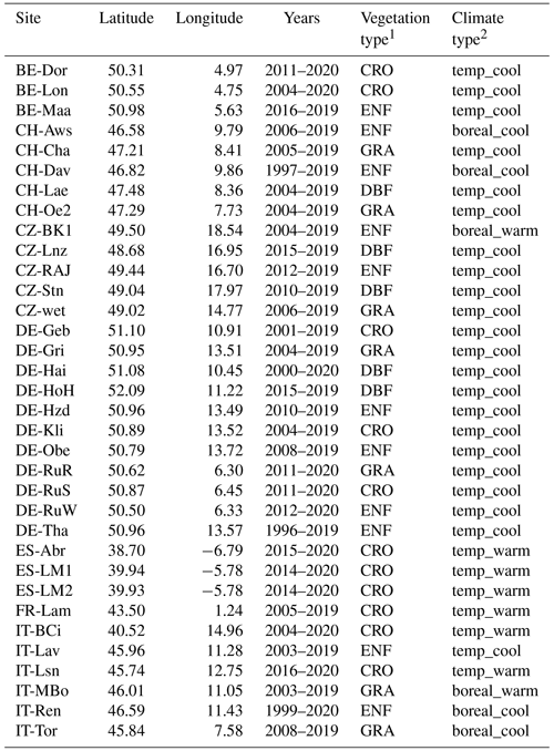
¹ Vegetation types are as follows: CRO – cropland; GRA – grassland; ENF – evergreen needleleaf forest; and DBF – deciduous broadleaf forest. ²Climate types are as follows: temp_warm – warm temperate climate; temp_cool – cool temperate climate; boreal_warm – cool boreal climate; and boreal_cool – cool boreal climate.

Appendix B: Sensitivity analysis and optimized parameters in twin DA experiments

The Morris method determines incremental ratios (i.e. elementary effects, EE), from which the mean (μ) and standard deviation (σ) for all the trajectories are calculated to assess the overall importance of each parameter. The μ values are used to rank the parameters in order to systematically discriminate between non-sensitive parameters (low μ values) and sensitive ones (high μ). The σ values are used to examine the non-linear effects and/or interactions with other parameters. To assess the results, we look at the normalized μ divided by the maximum μ corresponding to the most sensitive parameter. Thus, this results in a ranking built with values between 0 and 1, with 1 representing the most sensitive parameters and 0 representing parameters with no sensitivity (as shown in the colour bar of Fig. B1). Similarly, the σ values are normalized by the maximum μ. We select the parameters with an average (across LST constraints) normalized μ or normalized σ higher than 0.2. Figure B1 illustrates the 19 LST-related parameters of ORCHIDEE as a result of preliminary sensitivity analyses in the ES-Abr site for 2018, from which we identified 11 parameters (in bold in Table 1 in Sect. 2.3.2) to be optimized in the twin experiments.

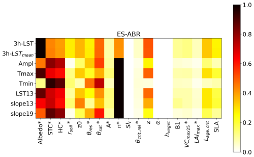
Figure B1 Morris sensitivity scores obtained in the different sensitivity analysis experiments performed for the ES-Abr site. The plot highlights the most influential key parameters, the various LST features studied, and their normalized importance. The LST features studied are as follows: the 3 h LST (3 h-LST) series (3 h-LST), daily mean LST (3 h-LST_mean), daily amplitude LST (Ampl), maximum (T_max) and minimum (T_min) LST, LST at 13:00 LT (LST13), and morning (slope13) and afternoon (slope19) gradients.

Appendix C: Twin experiments using actual CCI-LST availability and uncertainties

This approach allows us to conduct twin DA experiments resembling a real observation case, building upon the findings of the previous evaluation that utilized the full availability of pseudo-observations. For this purpose, the 3-  LST pseudo-observations, once filtered and perturbed with CCI-LST availability and uncertainties, are used to conduct two DA experiments with the GA method: assimilating the 3 h LST series alone (LST DA) and incorporating the T_max (LST + T_max DA). These two scenarios were kept because they showed the best results in the previous twin DA experiments. For both DA experiments, the RMSD values are comparable to those obtained when considering the full pseudo-data series, although larger, particularly for LE (Fig. C1). The best performance across all three variables (LST, LE, and H) is observed in the 3 h-LST + T_max DA experiment, with mean RMSD reductions of 65 %, 50 %, and 83 % for LST, LE, and H, respectively. It is noteworthy that the availability and noise introduced from CCI data have a more significant impact on LE compared with LST and H. Furthermore, assimilating 3 h LST alone occasionally results in some runs that increase errors for LE after the optimization. In terms of the optimized parameters, they agree with the optimization using the full pseudo-observation series, i.e. the most sensitive parameters align with the true parameter values with the exception of Albedo^* (Fig. C2). Despite this, the availability and uncertainties of CCI-LST data may significantly impact the estimation of daily maximum LST (T_max) – as well as the other characteristics – especially at sites characterized by climates with a lower occurrence of cloud-free conditions, unlike the Mediterranean site used in the twin experiment. Consequently, we will conduct the actual data DA experiments by only considering the entire 3 h CCI-LST series (LST DA).

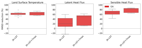
Figure C1 Box plots of the model–data RMSD reduction (%) for 30 min LST, LE, and H obtained within 16 optimization tests with random first-guess parameter values using the GA method in the twin experiments considering actual availability and uncertainties from CCI-LST data. The x axis indicates the experiment assimilating 3 h LST pseudo-observations: 3 h-LST only and 3 h-LST + T_max.

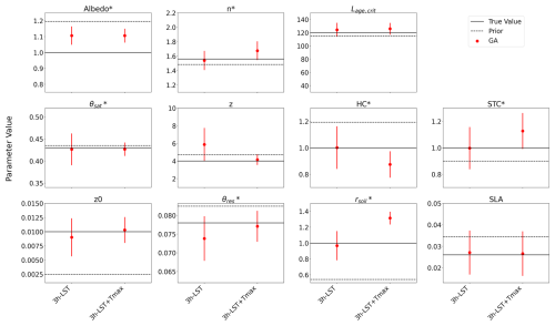
Figure C2 Parameter estimates for each twin experiment using the GA method considering actual availability and uncertainties of CCI data represented by the mean and standard deviation across 16 optimization tests with random first-guess parameter values. The x axis indicates the experiment assimilating 3 h LST pseudo-observations: 3 h-LST only and 3 h-LST + T_max. The true parameter (default ORCHIDEE value) and prior values (defined randomly) are represented by the solid horizontal lines and the dashed horizontal lines, respectively.

Appendix D: Decomposition of mean-square errors per site

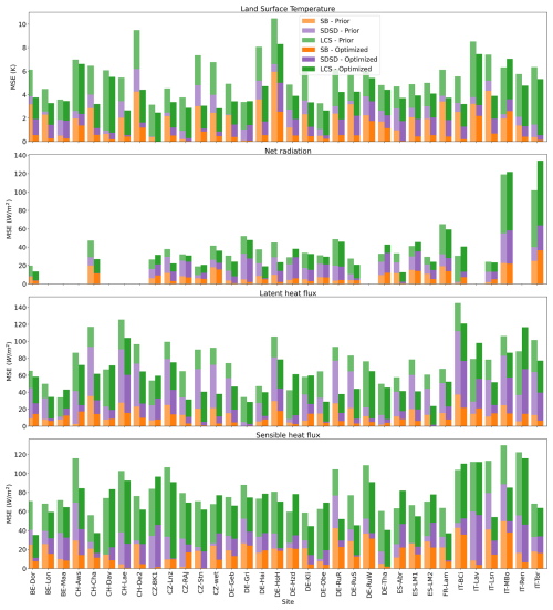
Figure D1 Decomposition of the MSE in terms of bias (SB), lack of correlation (LCS), and difference in the standard deviations (SDSD) between the model and observations over sites for LST, R_n, LE, and H. The light and dark bars represent the decomposition for Prior and Optimized simulations, respectively. LST observations are from 3 h CCI-LST data, whereas energy fluxes are from 30 min in situ observations.

Appendix E: Impact of the optimization period

Figure E1 Comparison of model performance in 2017 for 30 min LST, LE, and H when parameters are calibrated in 2018 only or for the entire period (2015–2020) over the selected site in Spain (ES-Abr). Box plots obtained within 16 optimization tests with random first-guess parameter values for the DA experiment using the gradient-based (in blue) and genetic (in red) methods in terms of the model–data RMSD. The DA experiment assimilates the daily mean, amplitude, and maximum LST.

Appendix F: Impact of assimilating LST on phenology

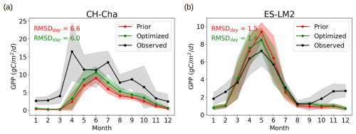
Figure F1 Annual cycle of GPP modelled for 2018 over a grassland (CH-Cha; a) and cropland (ES-LM2; b) site. The mean (dot) and standard deviation (shaded area) are represented for in situ observations (black) and for Prior (red) and Optimized (green) ORCHIDEE simulations. The RMSD on a daily basis (RMSD_day) against in situ observations is shown for Prior (red) and Optimized (green) simulations.

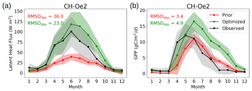
Figure F2 Annual cycle of LE (a) and GPP (b) modelled for 2018 over a cropland site (CH-Oe2); LE is improved, whereas GPP is degraded after assimilating CCI-LST data. The mean (dot) and standard deviation (shaded area) are represented for in situ observations (black) and for Prior (red) and Optimized (green) ORCHIDEE simulations. The RMSD on a daily basis (RMSD_day) against in situ observations is shown for Prior (red) and Optimized (green) simulations.