the Creative Commons Attribution 4.0 License.
the Creative Commons Attribution 4.0 License.
A scalable and modular reservoir implementation for large-scale integrated hydrologic simulations
Benjamin D. West
Reed M. Maxwell
Laura E. Condon
Recent advancements in integrated hydrologic modeling have enabled increasingly high-fidelity models of the complete terrestrial hydrologic cycle. These advances are critical for our ability to understand and predict watershed dynamics, especially in a changing climate. However, many of the most physically rigorous models have been designed to focus on natural processes and do not incorporate the effect of human-built structures such as dams. By not accounting for these impacts, our models are limited both in their accuracy and in the scope of the topics they are able to investigate. Here, we present the first implementation of dams and reservoirs in ParFlow, an integrated hydrologic model. Through a series of idealized and real-world test cases, we demonstrate that our implementation (1) functions as intended, (2) maintains important qualities such as mass conservation, (3) works in a real domain, and (4) is computationally efficient and can be scaled to large domains with thousands of reservoirs. Our results have the potential to improve the accuracy of current ParFlow models and enable us to ask new questions regarding conjunctive management of ground and surface water in systems with reservoirs.
- Article
(3138 KB) - Full-text XML
- BibTeX
- EndNote
Reservoirs are critical infrastructure and support water supply for agricultural, municipal, and commercial use; provide flood control benefits; generate power; support recreation; and more (Graf, 1999; Ho et al., 2017; Wisser et al., 2013). There are an estimated 91,000 dams in the continental US alone (Anon, 2017; Spinti et al., 2023). They drastically alter streamflow timing patterns, which impacts aquatic species, sediment transport, and water quality (Graf, 1999; Wisser et al., 2013). In many parts of the world, reservoirs are also projected to be under increasing amounts of strain as they struggle to meet increasing human demands and environmental needs, all under uncertain future conditions (Dettinger et al., 2015; Ho et al., 2017; Wisser et al., 2013; Zhou et al., 2018).
Given the widespread presence of reservoirs and their significant impact on stabilizing human water supplies and modifying river networks, it is imperative to have robust tools that can effectively represent reservoir operations within hydrologic systems at large scales. There is a large body of literature on reservoir operations and a long history of reservoir simulations (Blodgett, 2019; Dang et al., 2020; Haddeland et al., 2006; Hanasaki et al., 2006, 2022; Harbaugh, 2005; Kim et al., 2020; Müller Schmied et al., 2021; Shin et al., 2019; Sutanudjaja et al., 2018; Vanderkelen et al., 2022; Wada et al., 2014). Today, decision support models that are specifically designed to simulate networks of reservoirs and support decision-making processes are some of the most commonly used tools. Prominent examples include WEAP and RiverWare (Yates et al., 2005; Zagona et al., 2001). These models are tailored to address the complexities of interconnected reservoir systems and facilitate strategic planning and management of water resources. There also exist highly specialized model implementations of important areas. For example, Colorado's Decision Support System (Malers et al., 2012) represents all of the diversions and storage in the Colorado River system and is used for long-term planning.
While decision support models have very sophisticated abilities to represent the complexities of human operations, they generally rely on simplified representations of the physical hydrology. For example, WEAP and RiverWare represent reservoir networks as directional acyclic graphs, where each reservoir is associated with its own set of operating rules dictating the timing and volume of water releases. These models establish a flow pattern in which the outflow from one reservoir serves as the inflow for another reservoir, often incorporating time delays or other mechanisms to account for factors like irrigation use or other outflows from the system. This approach is good at capturing human-driven operations and decision-making aspects of reservoir networks but may not adequately account for the dynamics and complexities of the natural environment, especially under changing conditions.
On the other end of the spectrum, there is increasing focus on representing human operations in hydrologic models (i.e., models that were primarily designed to understand hydrologic systems). MODFLOW, WaterGAP, PCR-GLOBWB, and the National Water Model are all hydrologic models that now include reservoirs (Blodgett, 2019; Harbaugh, 2005; Kim et al., 2020; Müller Schmied et al., 2021; Sutanudjaja et al., 2018). These models handle the incorporation of reservoirs in a variety of ways. In the case of MODFLOW, it can be coupled with the decision support model MODSIM, which involves the addition of reservoir nodes to the stream network. These nodes account for the storage and release of water by exchanging information between MODFLOW and MODSIM at each time step (Valerio, 2000). PCR-GLOBWB and WaterGAP, on the other hand, estimate water use from various sources, including irrigation and reservoirs. They account for the water consumed by these sources by removing it from the system. Return flows, if any, are then reintroduced into the appropriate locations (Müller Schmied et al., 2021; Sutanudjaja et al., 2018). The National Water Model designates locations as lakes and reservoirs to track inflow. It utilizes parameterized functions such as weir or orifice functions to determine the amounts released from these reservoirs. These approaches are just a few prominent examples and are far from constituting an exhaustive list of hydrologic models. Many other models, such as VIC, CaMa-Flood, LEAF-Hydro, and mizuRoute, all contain reservoir representation (Vanderkelen et al., 2022).
Although reservoir operations have been added into many physical hydrology models, it is worth noting that they are still absent from fully integrated hydrologic models that solve the surface and subsurface systems simultaneously and account for variably saturated flow, like ParFlow and ATS (Coon et al., 2019; Kuffour et al., 2020; Maxwell et al., 2015; O'Neill et al., 2021). These models are very powerful because they solve physically based equations for water and energy fluxes for both the surface and subsurface at the same time. They are good at representing the vadose zone and can capture evolving systems. Integrated hydrologic models possess unique strengths in examining the intricate interactions between different components of the environment, especially under changing conditions. For instance, ParFlow has been used to investigate the connections between groundwater flow and transpiration partitioning (Maxwell and Condon, 2016).
Previous work using models that do have reservoirs shows that they can have significant impacts on the hydrologic cycle beyond their direct streamflow alterations. For example, in a NOAH-HMS model of the Poyang Lake basin, a 2.7 % increase in total evapotranspiration (ET) was observed, mostly attributed to direct ET from the reservoir surface (Wei et al., 2021). The same study also observed a slightly higher groundwater table which resulted in slightly wetter soils and a 0.7 % decrease in groundwater recharge due to the reduced hydraulic gradient at the surface. Globally, a WaterGAP model showed a reduction of discharges to oceans of 0.8 % due to ET that occurred from reservoir surfaces. Low flow rates also decreased by 10 % across a quarter of global land area due to reservoir releases redistributing flow temporally (Döll et al., 2009). Note that these studies exclude smaller reservoirs, which make up the majority of reservoirs but hold a minority of the overall storage. This exclusion may mean some effect sizes are underestimated.
Adding reservoir operations to integrated physical hydrology models would have several benefits. Perhaps most importantly, it would increase their accuracy in managed systems and expand the range of research questions that can be addressed with these models. Additionally, previous research has shown that reservoirs not only alter streamflow regimes but can have much more far-reaching impacts on the watershed as a whole (Graf, 1999; Hwang et al., 2021; Wei et al., 2021; Wisser et al., 2013; Zhou et al., 2018). Integrated hydrologic models could be useful tools to evaluate reservoir impacts on these complex integrations as they directly solve the underlying physics of the complete system. Lastly, they may be able to provide a new, generalizable understanding and characterization of reservoir operations, either through controlled experiments or inference based on existing data.
Here, we present the first reservoir module for the integrated hydrologic model ParFlow. Our initial implementation is quite simple, but it provides the scaffolding for future development. For example, in our reservoir parameterizations, we have intentionally selected fields that align with existing reservoir databases such as GRanD and ResOpsUS to facilitate future real-world simulations with these databases (Lehner, et al., 2011a, b; Steyaert et al., 2022; Maxwell et al., 2015). We focus on idealized test cases in this paper but demonstrate scaling out to a large number of reservoirs to demonstrate the feasibility of large-scale applications.
In the following sections, we provide detailed specifications on how reservoirs are represented within the ParFlow framework (Sect. 2.1–2.3) and how a model user can interact with the reservoir module that is developed here (Sect. 2.4). A proof of concept for the new reservoir module is demonstrated with four sets of test cases run on idealized domains, scaling from one reservoir up to 10 000 reservoirs (Sect. 3.1–3.4). Our scaling tests illustrate performance up to the national scale, demonstrating the feasibility of this approach for integration into large-scale simulations.
In this section, we provide a detailed description of the implementation of reservoirs in ParFlow. We start by explaining the basic functioning of ParFlow in Sect. 3.1. Then, we provide a high-level overview of the choices we made and the rationale behind them in Sect. 3.2. In Sect. 3.3, we illustrate how the reservoirs interact with ParFlow's grid via an Intake Cell and a Release Cell. Finally, in Sect. 3.4, we provide a comprehensive list of the fields needed to define a reservoir and demonstrate the user interface for incorporating reservoirs into a ParFlow model.
2.1 ParFlow
ParFlow is a gridded partial-differential-equation-based (PDE-based) hydrologic model that solves both the surface and subsurface flow systems simultaneously (Kollet and Maxwell, 2006; Kuffour et al., 2020; Maxwell et al., 2015). In the subsurface, ParFlow solves the mixed form of the Richards equation (Eq. 1) (Celia et al., 1990; Richards, 2004) for variably saturated flow, with a general source–sink term added to account for transpiration, wells, and other fluxes.
Here, h (L) is the pressure head, t is time, Ss (L−1) represents the specific storage, ϕ (–) denotes the porosity, Sw (–) represents the relative saturation, and qr (T−1) represents a general source–sink term. The flux term q (L T−1) is based on Darcy's law:
where Ks(x) (L T−1) represents the saturated hydraulic conductivity tensor; kr (–) represents the relative permeability; z (L) denotes the elevation; and θ represents the local angle of topographic slope between the relevant grid cells, with Sx and Sy denoting the slopes in the x and y directions, respectively. The angles θx and θy are calculated as and .
The van Genuchten (1980) relationships are employed for the relative saturation (Sw(h)) and permeability (kr(h)) functions (van Genuchten, 1980).
There are multiple solvers available for overland flow in ParFlow, including both the kinematic and diffusive wave equations. Our implementation of reservoirs works with the kinematic wave equation, which is derived by applying continuity equations to pressure and flux and uses Manning's equations for the depth-averaged velocity vsw (L T−1) (Kollet and Maxwell, 2006).
In the above, k is the unit vector in the upward (z) direction, and λ is a constant equal to the inverse of the vertical grid spacing. Note that the ||h,0|| operator means we must select the larger value between h and 0. This operator means that surface flow only occurs when pressure is greater than 0. The head used in the overland flow equation is the same as the head used in Eqs. (1) and (2). This free surface overland flow boundary condition allows for the integrated solution of the surface and subsurface.
Equations (1)–(3) are discretized onto a grid and solved in a non-linear, fully implicit fashion using a Newton–Krylov solver. This integrated, implicitly solved system allows for the correct resolution of interactions between surface and subsurface flow and mass conservation across the whole system.
More simply, because the surface and subsurface systems are solved in an integrated fashion, ParFlow also does not require the user to specify the location of a stream network a priori. Flow emerges when enough water has converged to result in surface pressures above zero. This type of approach is also taken by other integrated hydrologic models such as HydroGeoSphere (Brunner and Simmons, 2012).
Unfortunately, as reservoirs rely on large human-built infrastructure that is not statically situated (think the operating of the release gate), they do not emerge naturally in the same way as streams. Instead, our implementation of reservoirs makes extensive use of the source–sink terms in Eq. (3). Specifically, anthropogenic releases of water are added as source–sink flux terms to the top of the domain
2.2 Reservoir module overview
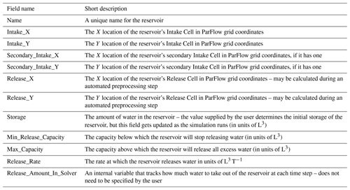
At the heart of our implementation is the addition of a reservoir module to ParFlow's code that enables the creation of reservoir objects. The use of a separate module allows us to start with a simple approach while building a framework that can easily be extended to more complicated formulations in the future. ParFlow models are built and run using model definition files, which may be written in either Python or Tcl. Reservoir objects can be added individually as model attributes in any language ParFlow supports or en masse through a CSV file using ParFlow's Python software development kit (SDK). Each reservoir object has a set of attributes (shown in Fig. 1) such as location and minimum and maximum capacity, along with a state variable that tracks its storage throughout the simulation.
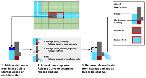
Figure 1Conceptual depiction of a reservoir's ParFlow grid. Here, we see how water comes off an Intake Cell and into Storage to be released later at the Release Cell in accordance with the reservoir's release curve.
In addition to the reservoir object, the module includes several new sub-processes that run to account for the intake and release of water from reservoirs. These sub-processes modify the functioning of the two grid cells, the Intake Cell and Release Cell, at which the reservoir is located (henceforth, all mentions of reservoir object fields will be denoted in uppercase italics to distinguish from cases in which we are simply discussing reservoirs broadly). At these locations, the reservoir module overrides ParFlow's normal physics to ensure that water only flows downstream when the reservoir's operating rule says there should be a release. Rule curves are used to determine the amount of water that should be released from the reservoir.
As illustrated in Fig. 1, at every time step, (1) water flows into the reservoir and the storage is updated, (2) the amount of water that is released from the reservoir is determined based on the reservoir's Storage, and (3) these releases are applied as fluxes at the Release Cell.
Our goal for our implementation was to choose a flexible representation that could represent a variety of use cases. ParFlow models are run at many scales, spanning hillslope-scale simulations up to continental models covering millions of square kilometers. Additionally, reservoirs are highly abundant and often do not have good data available regarding their operating rules. When data are available, there is not one consistent format or way of defining the operations that everyone uses. For these reasons, we prioritized simplicity and efficiency of implementation to establish a core set of functionalities that could easily be extended in the future as the reservoir data landscape shifts.
The representation we chose is also designed to be computationally efficient, making it feasible to scale up to national-scale simulations. By imposing fluxes directly in the cells, we avoid convergence issues associated with simulating the raising and lowering of the reservoir's stop gate. We also chose simple initial release curves, which enables us to develop a framework for adding more complex curves and to test how reservoirs impact runtime performance.
2.3 Intake and Release cells
As shown in Fig. 2, each reservoir has an Intake Cell and a Release Cell. The Release Cell is located directly downstream of the Intake Cell based on the topographic slopes. If a cell has multiple faces with outward slopes, the steepest gradient is selected to be designated as the Release Cell. It should be noted here that the Intake Cell is not intended to represent the inundated area of the reservoir or its bathymetry. It is the most downstream location in the reservoir, where we link the reservoir storage object to the grid. In this approach, we do not explicitly resolve the reservoir inundated area.
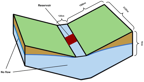
Figure 2Idealized illustration of the tilted-v test case adapted from Farley and Condon (2023). The domain is made up of grid cells, with each being m in size. This leads to each hillslope being 1500 m from the domain edge in relation to the channel. The slope along the channel is 0.01, while the slopes perpendicular to the channel are 0.1. The sides and bottom are no-flow boundaries.
To capture incoming water, we have implemented a process that iterates through all reservoir Intake Cells at each time step. This looping is achieved through ParFlow's concept of subgrids, which enables efficient parallelization. If a reservoir's Intake Cell has a pressure head h greater than zero, h is reset to zero, and the corresponding volume of water (calculated by Eq. 4) is added to the reservoir's storage:
where dx and dy are the grid cell dimensions in the x and y directions.
In some cases, a single Intake Cell is not sufficient. This occurs when channels are two cells wide, which can happen even for narrow channels under particular geometries. In these cases, a Secondary Intake Cell can be designated. Secondary Intake Cells function in the same way as other Intake Cells, with the water in them being diverted to the reservoir Storage. However, Secondary Intake Cells do not have associated Release Cells.
Release Cells also have special operations. At each time step, the reservoir module iterates over all the reservoirs and calculates how much water each should release based on the current storage and the reservoir release rules as follows: if a reservoir's storage is below its Min Release Capacity, no water is released. If its Storage exceeds its Max Release Capacity, all excess water is released. Otherwise, the release rate is determined by the reservoir's Release Rate attribute. The release flux is then added as a flux at each reservoir's Release Cell, and at the end of the time step, the release flux is removed from the reservoir's Storage. Note that, as ParFlow's solver is implicit, the size of release does not impose a constraint on the time step size. In this representation, any storage level below the Min Release Capacity is dead storage, and any storage above it is active storage. We do not explicitly represent flood storage. However, this is a feature that could be added in future implementations.
Even this simple release curve will allow for some useful simulations. However, the limited number of parameters used here does limit the complexity of operations that can be simulated. The module we have implemented here can easily be expanded to support a wide variety of release curves that may be needed for different applications. It would also be possible in the future to develop tools to read in release time series directly and bypass the rule curve approach entirely. This approach would allow for the direct simulation of datasets of historical releases.
2.4 Reservoir fields and user interface
As mentioned in Sect. 2.3, each reservoir is represented by an object that has multiple attributes and state variables. In order to add a reservoir to a model, the user must define these fields or they must be inferable from the other fields (as in the case of the location of the Release Cell). These fields may be seen in Table 1.
To add reservoirs with these fields to a model, users can follow one of two approaches. The first approach is to use the new ReservoirPropertiesBuilder class (henceforth referred to as the Builder) that we added to ParFlow's Python software development kit. This is expected to be the most common option for domains with more than one reservoir. To do this, users only need to provide the Builder with the location of a file containing their reservoir data, with one reservoir per line. The Builder will then add each row as a reservoir to the model. For an example snippet, refer to Fig. A1 in the Appendix.
Using the ReservoirPropertiesBuilder class to add reservoirs to a ParFlow model comes with several advantages besides concision. Namely, the class performs automatic preprocessing to calculate the locations of Release Cells, edit the slope files at Intake Cell locations appropriately, and check for errors such as the existence of multiple reservoirs in one cell. While these tools are available to users with non-Python model definitions such as Tcl, they require a separate Python script to be called before the model is run, whereas using the ReservoirPropertiesBuilder class handles these steps automatically. This Builder is one of the main ways we support an easy user experience.
The second approach to add reservoirs to a ParFlow model is to add each reservoir attribute one by one as model attributes in the ParFlow run script (either Tcl or Python). This approach is less concise, and each reservoir will require 8+ lines of code. However, it may be preferable for domains with a small number of reservoirs, and it allows users to add reservoirs to older workflows, such as models written in Tcl. An example snippet may be seen in Fig. A2.
Our goal with this user interface is to require as little overhead and manual intervention as possible. To this end, we have selected fields that align with existing reservoir databases such as GRanD and ResOpsUS (Lehner et al., 2011a, b; Steyaert et al., 2022). Furthermore, in accordance with our commitment to providing a smooth user experience, we plan to enable users to inform the Builder that they are using these formats, allowing it to read them directly and convert them automatically in addition to the other preprocessing tasks we are handling.
We implemented three types of test cases to demonstrate the performance of the new reservoir module. In Sect. 3.1, we present test cases conducted based on an idealized domain, where we verify the proper functioning of reservoirs in a simplified setting with known expected outcomes. In Sect. 3.2, we run an ensemble of conditions in this domain to verify that reservoirs respond as expected to perturbations. In Sect. 3.3, we add a reservoir to a real domain and show some analysis tools available for it. Lastly, in Sect. 3.4, we examine performance test cases to assess the computational impact of incorporating reservoirs into a domain.
3.1 Idealized test cases
Idealized test cases validate the functionality of various aspects of our reservoirs. Specifically, we aim to demonstrate that reservoirs release the appropriate amount of water according to their defined release curves, take in the correct amount of water, and maintain mass conservation within the domain. Furthermore, this case provides a qualitative illustration of how reservoirs respond to variations in domain parameters and how they impact streamflow.
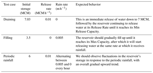
For the first test case, we simulate an idealized domain under three conditions: (1) draining, (2) filling, and (3) periodic rainfall. These cases represent common scenarios encountered by reservoirs and are designed to capture behaviors across the entire release curve. Tests were conducted on a simplified tilted-v domain, with a single reservoir placed midway down the channel, as illustrated in Fig. 2. The domain is 9.77 km2, roughly 1/10 the size of a typical HUC12 watershed (US Geological Survey, 2023).
We add a single reservoir to the domain with a Max Capacity of 7 MCM (million cubic meters) and a Min Release Capacity of 5 MCM. The reservoir is sized to hold roughly 1 year of precipitation in the domain. The Max Capacity equates to 28.24 in. (71.7 cm) of rainfall across the domain in a year, which is roughly equal to the annual rainfall in Minnesota (Kunkel, 2022). The minimum release capacity was set at 5 MCM. This is intentionally set relatively close to the Max Capacity to ensure that our test runs could easily achieve reservoir storage below the minimum capacity threshold. For both the Max and Min Capacity, the goal of our reservoir sizing is to choose reasonable values where our test cases can easily demonstrate correct behavior across the full range of operating scenarios.
The domain is discretized into 25 columns, 25 rows, and 2 layers, resulting in a total of 1250 grid cells (each grid cell is 125×125 m). The domain is homogenous, with a saturated hydraulic conductivity (K) value of 0.000001 m h−1 (a reasonable K value for clay). The slope along the channel is 0.01, and the slopes perpendicular to the channel are 0.1. This configuration effectively promotes the immediate runoff of water into and then down channel.
Zero-flux boundaries are applied along the bottom and sides of the domain. Rainfall is applied along the top boundary and varied based on the test case. A single reservoir was placed in the middle cell of the domain, which lies in the channel halfway down.
Table 2 describes the initial Storage, Release Rate, and Rain Rate for each of the three test cases, as well as the expected result.
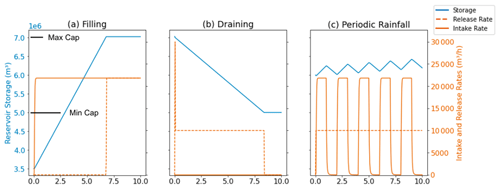
Figure 3Idealized test case results for the filling (a), draining (b), and periodic rainfall (c) cases. For each case, the reservoir's storage (blue line), intake rate (solid red line), and release rate (dashed orange line) are plotted as a function of time for the 10 h simulation. The reservoir's Max Capacity (Max Cap) and Min Release Capacity (Min Cap) are shown on the y axis of subplot (a).
Figure 3 shows the reservoir storage, intake rate, and release rate over time for all three test cases. Overall, the results align with the expected behavior described in Table 2. In the filling case (Fig. 3a), the storage of the reservoir increases until it reaches its Max Capacity. At this point, all incoming water is released, resulting in the release rate (dotted orange line) becoming equal to the intake rate (solid orange line). In the draining case (Fig. 3b), there is an initial surge in the release rate as excess water is discharged, which can be seen in the large early value reached by the dotted orange line. This is followed by a steady decline in storage (blue line) at the specified Release Rate until the Min Release Capacity is reached. Once the Min Release Capacity is attained, the reservoir ceases to release water. Lastly, in the periodic rainfall case in Fig. 3c, we observe fluctuations in reservoir storage (blue line) with upticks corresponding to when the intake rate (solid orange line) is positive and downticks corresponding to when there is no intake, with a gradual overall upward trend. We also note that, in the draining case (Fig. 6b), the amount of time it takes for the reservoir to empty is completely consistent with the reservoir's Release Rate, indicating that the internal storage is correctly accounted for.
Overall, Fig. 3 validates that the reservoirs are functioning as intended, adhering to the expected behaviors outlined in Sect. 2.2 and Table 2. These findings provide confidence in the accurate representation of the release curves across their entirety.
3.2 Ensemble case
Next, we conducted an ensemble of simulations on the idealized domain to (1) demonstrate the capability of reservoirs to handle a wide range of scenarios and (2) validate their expected behaviors in response to perturbations, ensuring that we have not designed something that only works in a narrow parameter range. The ensemble involved varying the Release Rates of the reservoir and the rain rates within the domain. A range of Release Rates from 0 to 0.01 MCM h−1 and rain rates from 0 (no rainfall) to 0.01 m h−1 (a heavy storm) were selected. For each combination of Release Rate and rain rate, the simulations were run for a duration of 1 d at an hourly time step. We initialized the reservoir with a Max Capacity of 5.5 MCM for all simulations to ensure consistency across the ensemble.
Figure 4 shows the relationship of reservoir storage at the end of the simulation to the release and rain rates. We anticipated a linear relationship between storage and both release and rain rates, leading to a plane-like surface in the 3-D plot. As expected, the plotted points exhibit this linear pattern, with higher rain rates corresponding to increased storage and lower Release Rates being associated with higher storage values. The simplicity of both our domain and our release curves is what drives the strong linearity observed in these relationships. Given more complex topography, rainfall patterns, and operating curves, this plot would be less linear.
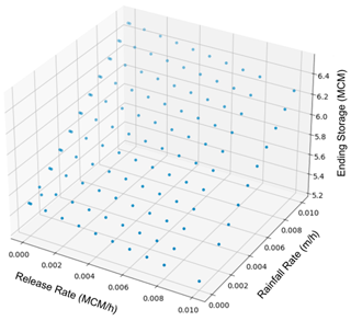
Figure 4Storage change after 1 d vs. rainfall and release rates. Each point represents one member of the simulation ensemble we used to conduct a sensitivity analysis of variables related to reservoir functioning. Points are shaded to help give a sense of depth.
To explore the relationship between rainfall and storage more quantitatively, we compare the rate of storage change in the reservoir to the maximum possible inflow. Maximum possible storage change is calculated as the total land area upstream of the reservoir multiplied by the rain rate. In practice, we do not expect the reservoir storage changes to be exactly equal to this maximum possible storage change because (1) not all water drains into the reservoir, (2) there can be time lags between precipitation and reservoir inflow, and (3) some of the precipitation will infiltrate into the subsurface. However, in this simple domain, we expect these values to be close.
Figure 5 plots the relationship between simulated storage change and maximum possible storage change. As expected, we see a linear relationship between storage change and maximum possible storage change that falls that slightly below the 1-to-1 line.
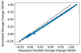
Figure 5A comparison of actual storage change after 1 d to the maximum possible daily storage change. The 1-to-1 line is shown in dashed black for reference.
This consistency with a simple mass balance indicates that, under a wide variety of conditions, reservoirs both take in and release the appropriate amount of water. This is further evidence that reservoirs are effective under a wide range of conditions and exhibit the desired behavior in response to variations in release and rain rates.
3.3 Real-world test case
Next, we conduct a test on a real domain, whose full description can be seen in Leonarduzzi et al. (2022). This test is intended to demonstrate that the implementation is robust enough to work in existing workflows and not just in idealized cases. It also shows that even very simple operating rules modify streamflow signals in the ways we know reservoirs do and demonstrates the method's ability to analyze water storage in a domain holistically.
The real domain we chose is the East–Taylor watershed. This 767 square-mile (1986 km2) watershed lies in the headwaters of the Colorado River, near the continental divide. It contains two rivers, the East and the Taylor, which converge right before they exit the domain, which can be seen in Fig. 6. The Taylor River is regulated by the Taylor Park Dam about halfway along its reach, while the East River is unregulated. This clear split between the regulated and unregulated tributaries makes for a natural comparison. The East–Taylor ParFlow domain was previously developed by Leonarduzzi et al. (2022), to which the reader is referred to for the full documentation.
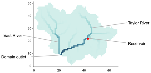
Figure 6A map of the East–Taylor watershed with the locations of the East River, the Taylor River, the reservoir, and the domain outlet noted.
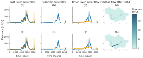
Figure 7Real-world test case results for both simulations. The top row (a–d) pertains to the case of adding a reservoir that never releases, while the bottom row (e–h) pertains to the case of a reservoir that releases at a constant rate. The fourth column (d, h) depicts the overland flow on the surface 2400 h into the simulations, with lighter, yellower shades representing more flow. The first, second, and third columns are hydrographs of the flow at different locations on the surface, with the blue lines representing the base case of no reservoir and the orange lines representing the simulation results. The first column (a, e) is the flow at the East River's outlet, the second column (b, f) is the flow at the reservoir's outlet, and the fourth column (c, g) is the Taylor River's outlet.
For our test cases, we add the Taylor Park Dam to the existing domain. We simulate two different modifications to the baseline run of the domain in 2003, which only simulates natural flow. In the first, we add a reservoir to where the Taylor Park Dam is; this releases no water at all. In the second, we have this same reservoir release water at the average inflow rate for 2003. In both cases, the reservoir is sized such that reaching either the minimum release storage or storage capacity was not a concern as the intent was to observe the effect of regulation on the domain and to ensure that the mass-accounting held up once more features, such as meteorological forcing, were turned on.
The results of the simulations can be seen in Fig. 7. In the case where no water is released, we can clearly see the reservoir blocking flow immediately downstream on the surface, with a gradual increase as one heads downstream as runoff accumulates from the drainage area downstream of the reservoir. The hydrograph at the reservoir outlet shows this as well, with an almost flat signal close to zero. Note that, in this case, there can still be some flow in the reservoir outlet flow that is contributed by cells downstream of the reservoir. Moving to the Taylor River domain outlet, we see a dampened signal compared to natural flow, with proportionally lower base and peak flows. Lastly, we see no change in the East River outlet flow, just as we expected.
In the case where we release water at a constant rate, the story is a bit different. At our selected time step, the flow downstream of the reservoir is higher than under naturalized conditions. This is because a time of low flow is being supplemented by a release of water. At the reservoir outlet, we again see a mostly flat signal but at the release rate and not at zero. Moving down to the Taylor River outlet, we now see a modulated flow signal, with higher baseflows but lower peaks. This type of modulation is exactly the effect reservoirs tend to have in reality. Lastly, we again see no change to the flow of the East River.
We also demonstrate an example storage analysis throughout the year in the domain for the simulation of a reservoir that releases at a constant rate, which can be seen in Fig. 8. Our module allows us to monitor changes in subsurface storage and in reservoir storage concurrently. Interestingly, for this domain, the changes in reservoir storage and subsurface storage throughout the year are of roughly the same magnitude.
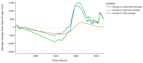
Figure 8A storage analysis for the simulation of a reservoir releasing at a constant rate. The blue line tracks the change in subsurface storage from the start of the year, the orange line tracks the change in reservoir storage from the start of the year, and the green line tracks the change in the sum of both of those storages.
These test cases demonstrate the proof of concept for our implementation in a real domain. Also, this shows that even adding a reservoir with the simplest possible operating impacts streamflow in a similar way to real reservoirs. Finally, we show that adding reservoirs in a domain allows for holistic analysis of water storage.
3.4 Performance scaling tests
Finally, we conduct a series of scaling tests to evaluate the computational cost associated with incorporating many reservoirs into a domain. These are crucial for understanding the potential impact on computing time as the number and complexity of experiments that can be conducted are often constrained by computational limitations. The primary aim of this test case is to demonstrate performance scaling as the number of unknowns increases.
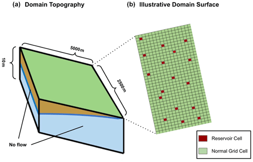
Figure 9Illustrative sloping-slab domain used for our performance test, adapted from Farley and Condon (2023). The left side (domain topography) shows the shape of the domain, while the right side (domain surface) depicts how reservoirs are scattered at random on the surface of the domain. The number of grid cells depicted is just illustrative for the sake of legibility. The actual domain size is cells, with the cells having dimensions of m. No-flow boundaries are set along the sides and bottom.
The performance tests were completed based on a sloping-slab domain (shown in Fig. 9) consisting of 500×500 grid cells in the x and y directions (625 000 lateral grid cells total) and two layers. The lateral resolution of the domain is 10 m, and the cell thickness is 5 m. Note that the fine spatial resolution (10 m) used here is just to simplify our experimental setup; our results would be the same if the grid sizing were larger. What is being tested here is the way the computational demand scales with the number of grid cells and the number of reservoirs applied. As with the first test domain, no-flow boundaries were applied on the bottom and sides of the domain, and a uniform saturated hydraulic conductivity value of 0.000001 m h−1 (typical of clay) was used for the entire subsurface. As with the previous test case, we are creating a relatively impermeable subsurface to promote runoff as we are really focusing on the surface system here. The same three physical cases from the first test case are used – draining, filling, and periodic rainfall – to investigate whether certain physical scenarios would result in significantly longer computing times.
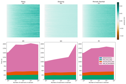
Figure 10The results of our performance scaling tests. The left column (a, d) correspond to the filling case, the center column (b, e) corresponds to the draining case, and the right column (c, f) corresponds to the periodic rainfall case. The top row (a–c) depicts the surface pressure at the end of the simulation when 10 000 reservoirs were placed in the domain. Water flows from left to right. The bottom row (d–f) depicts how simulation performance scales as reservoirs are added to the domain, with each component of the simulation shown in a different color.
For each case, we conducted eight simulations with an increasing number of reservoirs randomly placed throughout the domain, ranging from 0 to 10 000. We chose 10 000 reservoirs as this represents a number larger than any of the currently available datasets of historical releases for the US. Each simulation was run for a total of 10 h of simulation time. A range of simulation time components are tracked, including total simulation time, preprocessing time, time spent on the first time step, time spent on the second time step, and time spent on the subsequent time steps.
Figure 10 displays performance test results. The top row (Fig. 10a–c) depicts the ending surface pressures for each case for the scenario with 10 000 reservoirs added to the domain. Here, green indicates surface water, brown indicates a water table below the surface, white indicates a pressure near zero, and red indicates a reservoir's Intake Cell. In the filling case (Fig. 10a), reservoirs capture most of the rainfall that falls on the domain, and there are white streaks downstream of the reservoirs as they block flow. For the draining case (Fig. 10b), the domain is mostly saturated, except for the areas that are upstream of any reservoirs. In the draining case, there is no rainfall over the domain, and all the water comes from the reservoir releases (refer to Table 2). Finally, the periodic rainfall case (Fig. 10c) has the greatest spatial heterogeneity. Again, this is to be expected as reservoirs will fill and drain at different rates depending on their upstream areas and the presence of reservoirs upstream of them. In general, the streamflow increases from left to right across the domain as both reservoir releases and rainfall are aggregated moving downstream.
Figure 10d–f show the computational costs of each of the test cases for an increasing number of reservoirs. Overall, we show that the additional computational burden is not extreme for any of the cases. This is made apparent by noting the trend in the top-line height from left to right in Fig. 10d–f, which increases by ∼30 % for filling, ∼100 % for draining, and ∼15 % for periodic rainfall when 10 000 reservoirs have been added to the domain. In terms of the scaling, we note that the x axis is a log scale. This means that the mostly linear-looking increases are logarithmic, and the sharp jump in the draining case at 10 000 reservoirs represents an approximately linear increase.
There are some indications that costs in real simulations are likely to be smaller than this. The most extreme increase of ∼100 % is only seen when adding 10 000 reservoirs to the draining case. This results in a quick transition from an area that was drying up to one that was saturated and had some surface flow. This is an expensive physical situation to solve and only happens because of the extremely high density of reservoirs in the domain, which would never be seen in real models. Also, in all three domains, we see that the increase in cost mainly occurs in the later time steps. This indicates that the overhead to run the reservoir module is minimal, and the cost comes from increasing the physical complexity. Model runtimes are usually constrained by the most complex process to simulate. As this domain has very simple runoff patterns before reservoirs are added, the simulation of reservoirs is far more likely to increase the complexity and, therefore, the simulation runtimes. In real domains, it is far more likely that other complex physically based processes are occurring, and reservoirs are not the limiting factor.
It is also informative to look at the computational demand of the first and second time steps (shown in green and orange) as these are steps where we expect large changes as reservoirs are being activated. For instance, one might expect that the simultaneous activation of multiple reservoirs at the same time step could lead to slow convergence due to the resulting pattern of fluxes being applied. However, our results indicate that this is not the case and that there are no strong trends between the computational demand for the first and second time steps and the number of reservoirs applied. This is promising for future simulations of more realistic releases that vary in time.
Overall, these findings demonstrate that the reservoir module itself incurs minimal additional computational costs for the simulation, even for large numbers of reservoirs. Additionally, none of the components show non-linear performance degradation as we add reservoirs to the domain, except for the preprocessing in the largest case, which is likely to be due to machine limitations that could be alleviated by running on more cores. Furthermore, the overall degradation in performance time remains and is acceptable given that it is a one-time cost. This lack of degradation of the other components is promising as small performance changes can dominate behavior as problem sizes scale, causing even initially very cheap operations to cause significant overall slowdowns.
Still, it should also be noted that reservoir operations can create hydrologic conditions that take longer to address, as illustrated by the draining test case. Very large releases create sudden fluxes into the domain, which can be harder for the model to solve. Thus, we conclude here that the reservoir module scales well and does not add significant computational costs with runtime, which is crucial for supporting our goal of contiguous United States (CONUS)-scale simulations. However, depending on the reservoir configuration, reservoir releases can change computational demands significantly.
This paper presents a novel reservoir module for the integrated hydrologic model ParFlow, which has previously been unable to simulate reservoir operations. Our implementation takes a straightforward approach by overriding the physical behavior at two grid cells per reservoir. This enables the storage and timed release of water based on a reservoir's release curve and is in line with other physical hydrology models such as MODFLOW, WaterGAP, PCR-GLOBWB, and the National Water Model (Blodgett, 2019; Harbaugh, 2005; Müller Schmied et al., 2021; Sutanudjaja et al., 2018). We have also developed a user interface that simplifies the addition of reservoirs to a domain using a small number of input files that can be easily generated to cover domains with a large number of reservoirs.
The module presented here is fully integrated into the ParFlow code base and is designed to support future expansion. Potential future features include release curves that are time- or storage-dependent (i.e., parameters that vary monthly), release curves that call user-supplied models (e.g., a trained machine learning model), and automatic data loaders that can convert popular datasets like GRanD and ResOpsUS (Lehner et al., 2011a; Steyaert et al., 2022) into inputs to the reservoir module.
Test cases demonstrate that our implementation (1) functions as intended, (2) maintains important qualities such as mass conservation, (3) works in a real domain, and (4) is computationally efficient and can be scaled to large domains with thousands of reservoirs.
The new reservoir implementation provides two key advances. First, this may improve the ability of ParFlow models at any scale to match the streamflow in managed systems. This could improve the simulation performance, especially for large domains, and will allow new studies that consider management operations directly. Second, by implementing reservoirs into a fully integrated groundwater surface water model, we can facilitate new approaches to explore water management from a more holistic perspective, which is not possible with other models that already include reservoirs but simplify subsurface processes – for example, quantifying the role of vadose-zone exchanges in the hydrologic impacts shown with previous models (e.g., groundwater and soil moisture changes) (Döll et al., 2009; Wei et al., 2021), improving and generating reservoir rule curves via model inference, testing the impacts of hypothetical operation changes on the environment, and estimating the change falling groundwater levels could have on reservoir recharge in the future. Many of these topics require some combination of high physical realism and either large-scale simulations or large simulation ensembles. The approach presented here is uniquely positioned to support these types of analyses.

Figure A1A Python code snippet demonstrating how to add reservoirs from a file to a ParFlow model. In this case, the file is a CSV, but the Builder supports any of the file formats supported by ParFlow's TableToProperties class.
The reservoir module is available through the ParFlow repository. ParFlow, which has a broad development community, is available at https://doi.org/10.5281/zenodo.10989198 (Smith et al., 2024). Code for the idealized and performance test cases, which were developed by the authors, can be found at https://doi.org/10.5281/zenodo.14201537 (West et al., 2024). The model configuration for the real-world test case can be found at the same location. A description of the ParFlow configuration of the real-world test case, which was developed by a different set of authors, can be found in the original paper describing the domain (Hull et al., 2024).
Input data for the idealized and performance test cases can be found at https://doi.org/10.5281/zenodo.14201537 (West et al., 2024). Forcing data for the real-world test case are not publicly available, but a description of the configuration can be found in the original paper describing the domain (Hull et al., 2024).
Conceptualization: RMM, BW, and LEC. Formal analysis: BW, LEC, and RMM. Funding acquisition: LEC and RMM. Investigation: BW, LEC, and RMM. Methodology: BW, RMM, and LEC. Supervision: LEC and RMM. Visualization: BW and LEC. Validation: BW and LEC. Writing (original draft): BW and LEC. Writing (review and editing): BW and LEC.
The contact author has declared that none of the authors has any competing interests.
Publisher's note: Copernicus Publications remains neutral with regard to jurisdictional claims made in the text, published maps, institutional affiliations, or any other geographical representation in this paper. While Copernicus Publications makes every effort to include appropriate place names, the final responsibility lies with the authors.
This article is part of the special issue “Representation of water infrastructures in large-scale hydrological and Earth system models”. It is not associated with a conference.
The authors would like to acknowledge that AI was used in the writing process. Specifically, for early drafts, ChatGPT was asked to edit paragraphs for clarity and grammar. All of these were subsequently edited by us, and, in later drafts of the manuscript, all editing was done by the authors themselves.
This research has been supported by the US Geological Survey (grant no. G21AC10552).
This paper was edited by Sean Turner and reviewed by two anonymous referees.
Anon: Infrastructure Report Card: Dams, ASCEs 2021 Infrastruct. Rep. Card, https://www.infrastructurereportcard.org/wp-content/uploads/2016/10/2017-Infrastructure-Report-Card.pdf (last access: 20 November 2024), 2017.
Blodgett, D.: National Water Model V1.2 Retrospective and Operational Model Run Archive for Selected NWIS Gage Locations, USGS, https://doi.org/10.5066/P9ZRX948, 2019.
Brunner, P. and Simmons, C. T.: HydroGeoSphere: A Fully Integrated, Physically Based Hydrological Model, Groundwater, 50, 170–176, https://doi.org/10.1111/j.1745-6584.2011.00882.x, 2012.
Celia, M. A., Bouloutas, E. T., and Zarba, R. L.: A general mass-conservative numerical solution for the unsaturated flow equation, Water Resour. Res., 26, 1483–1496, https://doi.org/10.1029/WR026i007p01483, 1990.
Coon, E., Svyatsky, D., Jan, A., Kikinzon, E., Berndt, M., Atchley, A., Harp, D., Manzini, G., Shelef, E., Lipnikov, K., Garimella, R., Xu, C., Moulton, D., Karra, S., Painter, S., Jafarov, E., and Molins, S.: Advanced Terrestrial Simulator, US Department of Energy, https://doi.org/10.11578/DC.20190911.1, 2019.
Dang, T. D., Chowdhury, A. F. M. K., and Galelli, S.: On the representation of water reservoir storage and operations in large-scale hydrological models: implications on model parameterization and climate change impact assessments, Hydrol. Earth Syst. Sci., 24, 397–416, https://doi.org/10.5194/hess-24-397-2020, 2020.
Dettinger, M., Udall, B., and Georgakakos, A.: Western water and climate change, Ecol. Appl., 25, 2069–2093, https://doi.org/10.1890/15-0938.1, 2015.
Döll, P., Fiedler, K., and Zhang, J.: Global-scale analysis of river flow alterations due to water withdrawals and reservoirs, Hydrol. Earth Syst. Sci., 13, 2413–2432, https://doi.org/10.5194/hess-13-2413-2009, 2009.
Farley, A. and Condon, L. E.: Exploring the Signal Filtering Properties of Idealized Watersheds Using Spectral Analysis, Adv. Water Resour., 178, 104441, https://doi.org/10.1016/j.advwatres.2023.104441, 2023.
Graf, W. L.: Dam nation: A geographic census of American dams and their large-scale hydrologic impacts, Water Resour. Res., 35, 1305–1311, https://doi.org/10.1029/1999WR900016, 1999.
Haddeland, I., Skaugen, T., and Lettenmaier, D. P.: Anthropogenic impacts on continental surface water fluxes, Geophys. Res. Lett., 33, L08406, https://doi.org/10.1029/2006GL026047, 2006.
Hanasaki, N., Kanae, S., and Oki, T.: A reservoir operation scheme for global river routing models, J. Hydrol., 327, 22–41, https://doi.org/10.1016/j.jhydrol.2005.11.011, 2006.
Hanasaki, N., Matsuda, H., Fujiwara, M., Hirabayashi, Y., Seto, S., Kanae, S., and Oki, T.: Toward hyper-resolution global hydrological models including human activities: application to Kyushu island, Japan, Hydrol. Earth Syst. Sci., 26, 1953–1975, https://doi.org/10.5194/hess-26-1953-2022, 2022.
Harbaugh, A. W.: MODFLOW-2005: the U.S. Geological Survey modular ground-water model–the ground-water flow process, USGS, https://doi.org/10.3133/tm6A16, 2005.
Ho, M., Lall, U., Allaire, M., Devineni, N., Kwon, H. H., Pal, I., Raff, D., and Wegner, D.: The future role of dams in the United States of America, Water Resour. Res., 53, 982–998, https://doi.org/10.1002/2016WR019905, 2017.
Hull, R., Leonarduzzi, E., De La Fuente, L., Viet Tran, H., Bennett, A., Melchior, P., Maxwell, R. M., and Condon, L. E.: Simulation-based inference for parameter estimation of complex watershed simulators, Hydrol. Earth Syst. Sci., 28, 4685–4713, https://doi.org/10.5194/hess-28-4685-2024, 2024.
Hwang, H.-T., Lee, E., Berg, S. J., Sudicky, E. A., Kim, Y., Park, D., Lee, H., and Park, C.: Estimating anthropogenic effects on a highly-controlled basin with an integrated surface-subsurface model, J. Hydrol., 603, 126963, https://doi.org/10.1016/j.jhydrol.2021.126963, 2021.
Kim, J., Read, L., Johnson, L. E., Gochis, D., Cifelli, R., and Han, H.: An experiment on reservoir representation schemes to improve hydrologic prediction: coupling the national water model with the HEC-ResSim, Hydrolog. Sci. J., 65, 1652–1666, https://doi.org/10.1080/02626667.2020.1757677, 2020.
Kollet, S. J. and Maxwell, R. M.: Integrated surface–groundwater flow modeling: A free-surface overland flow boundary condition in a parallel groundwater flow model, Adv. Water Resour., 29, 945–958, https://doi.org/10.1016/j.advwatres.2005.08.006, 2006.
Kuffour, B. N. O., Engdahl, N. B., Woodward, C. S., Condon, L. E., Kollet, S., and Maxwell, R. M.: Simulating coupled surface–subsurface flows with ParFlow v3.5.0: capabilities, applications, and ongoing development of an open-source, massively parallel, integrated hydrologic model, Geosci. Model Dev., 13, 1373–1397, https://doi.org/10.5194/gmd-13-1373-2020, 2020.
Kunkel, K. E.: State Climate Summaries for the United States 2022, NOAA Technical Report NESDIS 150, NOAA NESDIS, https://statesummaries.ncics.org/chapter/mn/ (last access: 20 November 2024), 2022.
Lehner, B., ReidyLiermann, C., Revenga, C., Vorosmarty, C., Fekete, B., Crouzet, P., Doll, P., Endejan, M., Frenken, K., Magome, J., Nilsson, C., Robertson, J. C., Rodel, R., and Sindorf, N.: Global Reservoir and Dam Database, Version 1 (GRanDv1): Reservoirs, Revision 01, NASA, https://doi.org/10.7927/H4HH6H08, 2011a.
Lehner, B., Liermann, C. R., Revenga, C., Vörösmarty, C., Fekete, B., Crouzet, P., Döll, P., Endejan, M., Frenken, K., Magome, J., Nilsson, C., Robertson, J. C., Rödel, R., Sindorf, N., and Wisser, D.: High-resolution mapping of the world's reservoirs and dams for sustainable river-flow management, Front. Ecol. Environ., 9, 494–502, https://doi.org/10.1890/100125, 2011b.
Leonarduzzi, E., Tran, H., Bansal, V., De la Fuente, L., Condon, L. E., and Maxwell, R. M.: Training machine learning with physics-based simulations to predict 2D soil moisture fields in a changing climate, Front. Water, 4, 927113, https://doi.org/10.3389/frwa.2022.927113, 2022.
Malers, S. A., Bennett, R. R., and Nutting-Lane, C.: Colorado's Decision Support Systems: Data-Centered Water Resources Planning and Administration, 1–9, https://doi.org/10.1061/40499(2000)153, 2012.
Maxwell, R. M. and Condon, L. E.: Connections between groundwater flow and transpiration partitioning, Science, 353, 377–380, https://doi.org/10.1126/science.aaf7891, 2016.
Maxwell, R. M., Condon, L. E., and Kollet, S. J.: A high-resolution simulation of groundwater and surface water over most of the continental US with the integrated hydrologic model ParFlow v3, Geosci. Model Dev., 8, 923–937, https://doi.org/10.5194/gmd-8-923-2015, 2015.
Müller Schmied, H., Cáceres, D., Eisner, S., Flörke, M., Herbert, C., Niemann, C., Peiris, T. A., Popat, E., Portmann, F. T., Reinecke, R., Schumacher, M., Shadkam, S., Telteu, C.-E., Trautmann, T., and Döll, P.: The global water resources and use model WaterGAP v2.2d: model description and evaluation, Geosci. Model Dev., 14, 1037–1079, https://doi.org/10.5194/gmd-14-1037-2021, 2021.
O'Neill, M. M. F., Tijerina, D. T., Condon, L. E., and Maxwell, R. M.: Assessment of the ParFlow–CLM CONUS 1.0 integrated hydrologic model: evaluation of hyper-resolution water balance components across the contiguous United States, Geosci. Model Dev., 14, 7223–7254, https://doi.org/10.5194/gmd-14-7223-2021, 2021.
Richards, L. A.: Capillary conduction of liquids through porous mediums, Physics, 1, 318–333, https://doi.org/10.1063/1.1745010, 2004.
Shin, S., Pokhrel, Y., and Miguez-Macho, G.: High-Resolution Modeling of Reservoir Release and Storage Dynamics at the Continental Scale, Water Resour. Res., 55, 787–810, https://doi.org/10.1029/2018WR023025, 2019.
Smith, S., i-ferguson, Engdahl, N., FabianGasper, Chennault, C., Triana, J. S. A., Avery, P., Rigor, P., Condon, L., grapp1, Jourdain (Kitware), S., Bennett, A., gartavanis, reedmaxwell, Kulkarni, K., Bansal, V., xy124, alanquits, Beisman, J., elena-leo, Rooij, R. de, Swilley, J., DrewLazzeriKitware, Thompson, D., basileh, Coon, E., M.S, I. B., Azeemi, M. F., and Wagner, N.: parflow/parflow: ParFlow Version 3.13.0, Zenodo [code], https://doi.org/10.5281/zenodo.10989198, 2024.
Spinti, R., Condon, L., and Zhang, J.: The evolution of dam induced river fragmentation in the United States, Nat. Commun., 14, 3820, https://doi.org/10.1038/s41467-023-39194-x, 2023.
Steyaert, J. C., Condon, L. E. W. D., Turner, S., and Voisin, N.: ResOpsUS, a dataset of historical reservoir operations in the contiguous United States, Sci. Data, 9, 34, https://doi.org/10.1038/s41597-022-01134-7, 2022.
Sutanudjaja, E. H., van Beek, R., Wanders, N., Wada, Y., Bosmans, J. H. C., Drost, N., van der Ent, R. J., de Graaf, I. E. M., Hoch, J. M., de Jong, K., Karssenberg, D., López López, P., Peßenteiner, S., Schmitz, O., Straatsma, M. W., Vannametee, E., Wisser, D., and Bierkens, M. F. P.: PCR-GLOBWB 2: a 5 arcmin global hydrological and water resources model, Geosci. Model Dev., 11, 2429–2453, https://doi.org/10.5194/gmd-11-2429-2018, 2018.
US Geological Survey: National Hydrography Dataset, https://www.usgs.gov/national-hydrography/national-hydrography-dataset (last access: 5 July 2023), 2023.
Valerio, A. M.: Modeling groundwater-surface water interactions in an operational setting by linking riverware with modflow, https://riverware.org/PDF/Theses-PhD/Valerio-PhD.pdf (last access: 20 November 2024), 2000.
Vanderkelen, I., Gharari, S., Mizukami, N., Clark, M. P., Lawrence, D. M., Swenson, S., Pokhrel, Y., Hanasaki, N., van Griensven, A., and Thiery, W.: Evaluating a reservoir parametrization in the vector-based global routing model mizuRoute (v2.0.1) for Earth system model coupling, Geosci. Model Dev., 15, 4163–4192, https://doi.org/10.5194/gmd-15-4163-2022, 2022.
van Genuchten, M. T.: A Closed-form Equation for Predicting the Hydraulic Conductivity of Unsaturated Soils, Soil Sci. Soc. Am. J., 44, 892–898, https://doi.org/10.2136/sssaj1980.03615995004400050002x, 1980.
Wada, Y., Wisser, D., and Bierkens, M. F. P.: Global modeling of withdrawal, allocation and consumptive use of surface water and groundwater resources, Earth Syst. Dynam., 5, 15–40, https://doi.org/10.5194/esd-5-15-2014, 2014.
Wei, J., Dong, N., Fersch, B., Arnault, J., Wagner, S., Laux, P., Zhang, Z., Yang, Q., Yang, C., Shang, S., Gao, L., Yu, Z., and Kunstmann, H.: Role of reservoir regulation and groundwater feedback in a simulated ground-soil-vegetation continuum: A long-term regional scale analysis, Hydrol. Process., 35, e14341, https://doi.org/10.1002/hyp.14341, 2021.
West, B. D., Maxwell, R. M., and Condon, L. E.: Reservoir Test Cases for ParFlow, Zenodo [code], https://doi.org/10.5281/zenodo.14201537, 2024.
Wisser, D., Frolking, S., Hagen, S., and Bierkens, M. F. P.: Beyond peak reservoir storage? A global estimate of declining water storage capacity in large reservoirs, Water Resour. Res., 49, 5732–5739, https://doi.org/10.1002/wrcr.20452, 2013.
Yates, D., Sieber, J., Purkey, D., and Huber-Lee, A.: WEAP21 – A Demand-, Priority-, and Preference-Driven Water Planning Model, Water Int., 30, 487–500, https://doi.org/10.1080/02508060508691893, 2005.
Zagona, E. A., Fulp, T. J., Shane, R., Magee, T., and Goranflo, H. M.: Riverware: A Generalized Tool for Complex Reservoir System Modeling1, J. Am. Water Resour. Assoc., 37, 913–929, https://doi.org/10.1111/j.1752-1688.2001.tb05522.x, 2001.
Zhou, T., Voisin, N., Leng, G., Huang, M., and Kraucunas, I.: Sensitivity of Regulated Flow Regimes to Climate Change in the Western United States, J. Hydrometeorol., 19, 499–515, https://doi.org/10.1175/JHM-D-17-0095.1, 2018.


