Towards a robust hydrologic data assimilation system for hurricane-induced river flow forecasting

The Hybrid Ensemble and Variational Data Assimilation framework for Environmental Systems (HEAVEN) is a method developed to enhance hydrologic model predictions while accounting for different sources of uncertainties involved in various layers of model simulations. While the effectiveness of this data assimilation in forecasting streamflow has been proven in previous studies, its potential to improve flood forecasting during extreme events remains unexplored. This study aims to demonstrate this potential by employing HEAVEN to assimilate streamflow data from United States Geological Survey (USGS) stations into a conceptual hydrologic model to enhance its capability to forecast hurricane-induced floods across multiple locations within three watersheds in the southeastern United States. The Sacramento Soil Moisture Accounting (SAC-SMA) hydrologic model is driven by two variables: precipitation and potential evapotranspiration (PET), collected from North American Land Data Assimilation System phase 2 (NLDAS-2) and Moderate Resolution Imaging Spectroradiometer (MODIS) satellite data, respectively. We validated the probabilistic streamflow predictions during five instances of hurricane-induced flooding across three regions. The results show that this data assimilation approach significantly improves the hydrologic model's ability to forecast extreme river flows. By accounting for different sources of uncertainty in model predictions – in particular model structural uncertainty (in addition to model parameter uncertainty) and atmospheric forcing data uncertainty – HEAVEN emerges as a powerful tool for enhancing flood prediction accuracy. The study found that data assimilation improved streamflow forecasting during Hurricane Harvey, enhancing the SAC-SMA model's accuracy across most USGS stations on the peak flow day. However, data assimilation had little effect on streamflow forecasting for Hurricane Rita. In Rita, the streamflow surged dramatically in a single day (from 28 to 566 m³ s⁻¹), causing the model to miss the high-flow event despite accurate initialization the day before. For hurricanes Ivan and Matthew, data assimilation improved peak flow forecasts by 21 % to 46 % in Mobile and 5 % to 46 % in Savanah, with improvements varying by station location.

1 Introduction

Floods rank among the most devastating and destructive natural calamities globally, annually causing significant economic losses and fatalities. According to the United Nations, flooding alone affected 2.3 billion people globally from 1995 to 2015 (Wahlstrom and Guha-Sapir, 2015). The literature indicates that climate change will amplify the magnitude and frequency of river flooding across the United States (Mallakpour and Villarini, 2015; Alipour et al., 2020b). This is due to the warming climate that leads to more evaporation from land and the ocean, which in turn increases the size and frequency of heavy-precipitation events and, therefore, escalates flooding risk (Alipour et al., 2020a; Blöschl et al., 2019).

A flood modeling system is indispensable for increasing the resiliency of communities prone to flooding by minimizing and mitigating its consequences and impacts. Developing an accurate and reliable flood forecasting and inundation system requires multiple components, including (1) a numerical weather prediction model to estimate atmospheric forcing variables such as precipitation, (2) a hydrological model to simulate the rainfall–runoff process and other hydrologic fluxes such as streamflow, and (3) a hydrodynamic model to route streamflow and map flood inundation (Grimaldi et al., 2019; Jafarzadegan et al., 2023). Hydrologic and hydrodynamic models together constitute a pivotal part of the flood inundation mapping task, which enables decision-makers to execute safe urban planning and operational risk management (Annis et al., 2020; Zischg et al., 2018). Existing literature reveals numerous studies concentrating on rainfall–runoff processes and floodplain dynamics, as well as the development of integrated hydrologic and hydrodynamic models. These efforts aim to enhance flood forecasting, assess flood risks, and model flood hazards across spatiotemporal scales (e.g., Felder et al., 2017; Laganier et al., 2014; Mai and De Smedt, 2017; Nguyen et al., 2016; Sindhu and Durga Rao, 2017; Tripathy et al., 2024).

Flood predictions and inundation maps are often inaccurate and erroneous due to different sources of uncertainties involved in different layers of the modeling chain (Ahmadisharaf et al., 2018; Annis et al., 2020; Apel et al., 2004). These include the hydraulic model structure, parameters (e.g., channel and floodplain roughness values), and boundary conditions (that is, upstream and downstream river discharge). While many studies underscore the significance of addressing uncertainties associated with channel and floodplain friction parameters (Aronica et al., 2002; Bates et al., 2004; Papaioannou et al., 2017; Pappenberger et al., 2005; Werner et al., 2005), channel geometry (Bhuyian et al., 2015; Neal et al., 2015), model structure (Dimitriadis et al., 2016; Liu et al., 2019; Petroselli et al., 2019), and input digital elevation model (DEM) resolution (Petroselli et al., 2019) in assessing the uncertainty in inundation mapping, little attention has been given to uncertainties within the hydrologic processes directly impacting flood modeling performance. In most of these studies, the hydrological uncertainties are related to the rating curves (Bermúdez et al., 2017; Di Baldassarre and Montanari, 2009; Domeneghetti et al., 2012; Pappenberger et al., 2006) and the shape of the flow hydrographs (Domeneghetti et al., 2013; Scharffenberg and Kavvas, 2011; Savage et al., 2016), but they do not explicitly account for the uncertainty associated with different components of the hydrologic model predictions, such as the forcing data uncertainty (due to the limitation of measurements and spatiotemporal representativeness of the data), model parameter uncertainty (due to conceptualization of the model and non-uniqueness of parameters), model structural uncertainty (due to the imperfect representation of a real system) (Pathiraja et al., 2018a; Parrish et al., 2012), and initial and boundary condition uncertainty (Abbaszadeh et al., 2018; Moradkhani et al., 2019). This study seeks to account for all the aforementioned sources of uncertainties involved in hydrologic model predictions within a Bayesian framework and studies their impacts on hurricane-induced extreme river discharges across different regions in the southeastern United States (SEUS). It is expected that reducing hydrologic uncertainties results in improving the accuracy and reliability of flood inundation mapping when the enhanced hydrologic forecasts are utilized to drive the hydrodynamic model.

Bayesian methods have been extensively utilized in numerous studies to characterize, quantify, and reduce the uncertainties in hydrologic model predictions (Abbaszadeh et al., 2020; DeChant and Moradkhani, 2012; Kuczera and Parent, 1998; Marshall et al., 2004; Moradkhani et al., 2005; Pathiraja et al., 2018b; Yan and Moradkhani, 2016). Data assimilation (DA) is a well-received Bayesian approach in the hydrometeorological community and is used to account for the uncertainties involved in different components of hydrologic model predictions by probabilistically conditioning the states of the model on observations (Moradkhani et al., 2005; Liu and Gupta 2007; Clark et al., 2008; Vrugt et al., 2006; Moradkhani et al., 2019; Abbaszadeh et al., 2018). DA methods based on the ensemble Kalman filter (EnKF) and particle filter (PF) are commonly used to recursively estimate both states and parameters. In these methods, Monte Carlo sampling and sequential updating are applied to not only a vector of model parameters but also a set of prognostic and diagnostic state variables at each assimilation step (see Moradkhani et al., 2019, and references therein). The probability distributions of both model states and parameters are recursively and independently updated at each time step as new observations become available. These approaches yield more accurate state and parameter estimates compared to open-loop simulations (without data assimilation), allowing the modeling system to evolve consistently over time. As a result, this leads to improved model predictions while accounting for uncertainties (Yan et al., 2015; Plaza et al., 2012; Hain et al., 2012; Lee et al., 2011; Lievens et al., 2016; DeChant and Moradkhani 2012, 2011; Abbaszadeh et al., 2018; Montzka et al., 2013; Koster et al., 2018).

In this study, we utilize a recently developed state-of-the-art hydrologic data assimilation method, hereafter referred to as the Hybrid Ensemble and Variational Data Assimilation framework for Environmental Systems (HEAVEN), to address all sources of uncertainties (i.e., forcing data, parameters, model structure, and initial conditions) in hydrologic simulations (Abbaszadeh et al., 2019). In particular, we study its usefulness and effectiveness in enhancing peak flow forecasts during an extreme event. Although the capability of this method, in conjunction with hydrological models for streamflow forecasting, has been demonstrated in previous studies, its ability to capture peak flows induced by heavy rainfall from hurricanes – common in southeastern regions – has not been explored. This study aims to address this gap and contribute to enhancing the resiliency of the SEUS, a region particularly vulnerable to extreme flooding due to hurricanes and tropical cyclones. By improving streamflow forecasting during such events, the study seeks to better inform flood management strategies and mitigate the impacts of future extreme weather events in these high-risk areas. The remainder of the paper is organized as follows. In Sect. 2, we present the materials and methods, encompassing the study areas and datasets, descriptions of the hydrologic model, data assimilation, and calibration methods. Section 3 examines the results of the hydrologic data assimilation and its advantages in enhancing peak flow forecasts. Section 4 outlines the conclusions and provides suggestions for further expanding this research in the future.

2 Materials and methods

This section first describes study areas and datasets used in this study, then introduces the hydrologic model that is used for streamflow prediction, and finally provides a summary for the model calibration and data assimilation methods.

2.1 Study areas

This study is conducted over three watersheds in three different states in the southeastern US. Figure 1 illustrates their geographical locations along with all the available United States Geological Survey (USGS) stations within those regions. Galveston, Mobile, and Savanah are the three watersheds located in hurricane-prone regions near the coast in the states of Texas, Alabama, and Georgia, respectively. These three watersheds encompass Galveston Bay, Mobile Bay, and Savanah Bay, respectively.

Figure 1 Location of Galveston, Mobile, and Savanah watersheds in three different states in the southeastern US. Black points represent the USGS stations operated in each watershed.

To provide a comprehensive analysis and show the robustness of the proposed approach in accounting for the uncertainties involved in hydrologic predictions and its benefits in generating accurate and reliable flood-inundated areas, we conducted this study over five hurricane-induced flooding events in three different regions in the SEUS. These include hurricanes Harvey and Rita (in the Galveston Watershed), Hurricane Ivan (in the Mobile Watershed), and hurricanes Matthew and Irma (in the Savanah Watershed). The Galveston Watershed comprises nine hydrologic unit codes (HUCs, i.e., HUC8s), including 12040202 (East Galveston Bay), 12040203 (North Galveston Bay), 12040102 (Spring), 12040103 (East Fork San Jacinto), 12040201 (Sabine Lake), 12040204 (West Galveston Bay), 12040205 (Austin–Oyster), 12040101 (West Fork San Jacinto), and 12040104 (Buffalo–San Jacinto). The climate in this region is humid subtropical with prevailing winds from the south and southeast that bring heat from the deserts of Mexico and moisture from the Gulf of Mexico. This watershed has a long, hot, and humid summer such that temperatures exceed 32 °C in August, while the winter is often mild, with temperatures that do not usually drop below 4 °C. Snowfall in Galveston is generally rare, while rainfall is frequent. With an average of 1000 mm, the rainfall is higher than the national average (767 mm). Hurricanes and tropical storms are notorious for wreaking havoc on the region's economy and environment and putting several communities at risk, including Houston, which is the fifth-largest metropolitan region in the US. In August 2017, Hurricane Harvey, characterized by heavy rainfall and wind storms, hit the Galveston area and caused significant flooding. Many locations around the bay area (i.e., Harris and Galveston counties) experienced more than 760 mm of rain in a few days, which resulted in USD 23 billion in property damages, according to Reuters (McNeill and Wilson, 2017). In September 2005, Hurricane Rita swept through eastern Texas and the Louisiana coast and resulted in extensive flooding, damages, and more than a hundred fatalities. Rita is the most intense tropical cyclone in the history of the Gulf of Mexico. According to the National Oceanic and Atmospheric Administration (NOAA) (Knabb and Brown, 2006), Rita's wind storm resulted in some flooding across the river networks in northern regions of the Galveston Bay by pushing the river water southward.

The Mobile Watershed refers to only the lower portion of the Mobile Basin, which consists of four HUC8s, including 03150204 (lower Alabama), 03160204 (Mobile–Tensaw), 03160205 (Mobile Bay), and 03160203 (lower Tombigbee). This region is characterized by a warm and temperate climate with well-distributed high rainfall throughout the year. Even in the driest month of the year, this area experiences significant rainfall. The precipitation is usually in the form of rain such that on average the annual rainfall reaches 1600 mm – almost 2 times more than the US average rainfall per year. In this watershed, summer is long and hot, and winter is short and cold. In the warmest and coldest months of the year, the temperature usually does not rise above 32 °C and does not fall below 5 °C. In September 2004, Hurricane Ivan made landfall along the coasts from Destin in the Florida Panhandle westward to Mobile Bay (Baldwin County), Alabama, according to NOAA (2005). The rainfall of this hurricane caused major flooding in both Alabama and northwestern Florida. According to the National Weather Service (https://www.weather.gov/mob/ivan, last access: 15 August 2024), Ivan resulted in nearly USD 14 billion in damage in both states. The radar-estimated data show the rainfall associated with Hurricane Ivan over the coastline of Alabama (near Orange Beach) reached more than 381 mm and then gradually decreased as the hurricane's eye moved northward.

The third watershed used in this study is Savanah, which is comprised of four HUC8s, including 03060106 (middle Savanah), 03060109 (lower Savanah), 03060110 (Calibogue Sound–Wright River), and 03060204 (Ogeechee Coastal). This watershed has a humid subtropical climate with long, hot summers and temperate winters. In this region, the precipitation is mainly influenced by the Atlantic Ocean (from the east side) and the Appalachian Mountains (from the west side). The precipitation is usually in the form of rainfall throughout the year with some rare snowstorms that occur in the northern mountainous regions in winter. Climate change has a serious impact on Savanah because of the severe heat and intense storms that cause periods of drought and flood, putting the region's water and food supplies at risk (Ingram et al., 2013; Knox and Mogil 2020). The temperature usually does not go below 4 °C and over 34 °C in the coldest and warmest months of the year, respectively. November and August are the driest and wettest months of the year, with an average precipitation of 61 and 183 mm, respectively. As shown in Fig. 1, the predominant land cover in Savanah is wetlands. In October 2016, Hurricane Matthew, characterized by with strong winds and heavy rainfall, hit the coastline of South Carolina and North Carolina and caused extensive coastal and inland flooding. The National Hurricane Center (NHC) reported dozens of deaths and USD 10 billion in damages across the US East Coast (Stewart, 2017). According to NOAA, Hurricane Matthew produced a copious amount of rain that led to record-breaking river levels in some locations in the Savanah region (Di Liberto, 2016). A year later, in September 2017, this region was hit again by Category 5 Hurricane Irma. The hurricane's wind speed exceeded 96.6 km h⁻¹ (60 mph) in the Savanah region, which resulted in a significant tidal surge in the Savanah River, according to the National Weather Service. The storm surge and tide together produced maximum inundation levels of 0.91 to 1.52 m (3 to 5 ft) above ground level along the coast of Georgia and much of South Carolina, inflicting extensive damage on infrastructure, agriculture, and properties.

2.2 Datasets

We used Moderate Resolution Imaging Spectroradiometer (MODIS) potential evapotranspiration (PET) and phase 2 of the North American Land Data Assimilation System (NLDAS-2) precipitation forcing data to drive the hydrologic model and estimate the streamflow. The streamflow observations collected from the USGS stations were used for calibration, assimilation, and validation purposes. To collect the USGS streamflow data, we used Climata (https://github.com/heigeo/climata, last access: 2 June 2025), which is a Python package that facilitates the acquisition of climate and water flow data from a variety of organizations such as NOAA, the National Weather Service (NWS), and USGS. The documentation for this package, along with example scripts, is available on Earth Data Science (2021).

2.2.1 MODIS

The MODIS global evapotranspiration product MOD16 is a gridded land surface ET dataset for global land areas at 8 d, monthly, and annual intervals (Mu et al., 2011, 2007). The output variables of the MOD16 product include 8 d, monthly, and annual ET; λE (latent heat flux); potential ET (PET); PλE (potential λE); and ET_QC (quality control). In this study, we used the MOD16A2 PET product at a 500 m spatial resolution and an 8 d time interval. Note that the pixel values for PET are the sum of all 8 d within the composite period. The dataset can be retrieved from https://lpdaac.usgs.gov/products/mod16a2v006/ (last access: 2 June 2025).

2.2.2 NLDAS-2

NLDAS-2 contains quality-controlled and spatially and temporally consistent meteorological forcing data, such as surface downward shortwave radiation, surface downward longwave radiation, specific humidity, air temperature, surface pressure, near-surface wind in u and v components, and precipitation rate. In this study, we used precipitation data from the NLDAS_FORA0125_H product, which has been widely used to derive hydrology and land surface models. This dataset is available from 1979 to the present with a spatial resolution of $\mathrm{1}/\mathrm{8}$° and temporal resolution of 1 h (Xia et al., 2012). These data can be retrieved from https://lpdaac.usgs.gov/products/mod16a2v006/ (last access: 2 June 2025).

2.3 SAC-SMA hydrologic model

In this study, we used the Sacramento Soil Moisture Accounting (SAC-SMA) model to simulate the streamflow at several locations within three different watersheds. SAC-SMA (Burnash et al., 1973) is a lumped-parameter model that represents each basin vertically through two soil zones: an upper zone and a lower zone (Gourley et al., 2014). The upper and lower zones represent the short-term storage capacity and long-term groundwater storage, respectively. For descriptions of model parameters and state variables, we refer readers to our previous study (Burnash et al., 1973; Abbaszadeh et al., 2018). This model is widely used by NOAA/the NWS for operational flood forecasting in the US (Smith et al., 2003; Lee et al., 2016; Kratzert et al., 2018; Gourley et al., 2014). SAC-SMA produces daily streamflow from daily PET and precipitation data. It is noted that here we disaggregated and aggregated the MODIS PET and NLDAS precipitation data, respectively, to 6 h intervals in order to be consistent with the SAC-SMA hydrologic model that generally runs at a 6 h time step. The SAC-SMA model inputs include 6 h mean areal precipitation (MAP) and 6 h mean areal potential evapotranspiration (MAPE). These variables are calculated by delineating the drainage area contributing to each USGS station where the hydrologic model is applied.

In this study, we employ the SAC-SMA model to simulate flooding events triggered by hurricanes occurring post-2001, as the MODIS-derived PET data necessary to drive the hydrologic model are available starting from 2001. Recent studies (Bennett et al., 2019; Bowman et al., 2017) have shown that using MODIS PET as input to the SAC-SMA model results in more reliable streamflow simulations compared to traditional evapotranspiration (ET) demand.

2.4 Data assimilation

In this study, we use the Hybrid Ensemble and Variational Data Assimilation framework for Environmental Systems (HEAVEN; Abbaszadeh et al., 2019) to account for all sources of uncertainties involved in the hydrologic model simulations. HEAVEN is a data assimilation method built through the combination of a deterministic four-dimensional variational (4D-Var) assimilation method with the PF ensemble data assimilation system. Since we have already provided a comprehensive description of this data assimilation approach in Abbaszadeh et al. (2019), here we briefly describe its formulation and implementation process. HEAVEN provides the possibility that both sequential and variational assimilation approaches can effectively feed each other in a single framework to produce a more complete representation of posterior distributions. The first step is to minimize the weak-constraint 4D-Var cost function (Eq. 1) within an assimilation cycle and find the optimal initial condition, which is also known as analysis x_a. For the time period T and assimilation window size K ($[t_{\mathrm{0}},t_{k=K}])$, the number of assimilation cycles in HEAVEN becomes $T/K$. For example, for a 1-year analysis period of T = 365 d, with the assumption of K = 5 d, 73 assimilation cycles or windows are defined. In each assimilation cycle, k ranges between 0 and K, where k=0 indicates the initial time step. The optimal solution is the joint maximum likelihood estimate of the state variables within the assimilation window given the observations. The only free variable in the minimization of the cost J is the model state x₀ at the initial time t₀. The optimal solution (analysis) is obtained through an iterative method that typically relies on linearized versions of the model and observational operator to obtain a quadratic approximation to the cost J (outer iteration) and adjoint modeling for gradient information.

$$\begin{array}{}\text{(1)}& \begin{array}{rl}J(x_{\mathrm{0}},\mathrm{\dots },x_K)=& J^{\mathrm{b}}+J^{\mathrm{o}}+J^{\mathrm{q}}\\ =& {\displaystyle \frac{\mathrm{1}}{\mathrm{2}}}(x_{\mathrm{0}}-x_{\mathrm{0},\mathrm{b}}{)}^{\mathrm{T}}{B}^{-\mathrm{1}}(x_{\mathrm{0}}-x_{\mathrm{0},\mathrm{b}})\\ & +{\displaystyle \frac{\mathrm{1}}{\mathrm{2}}}\sum _{k=\mathrm{0}}^K(y_k-h_k(x_k\left){)}^{\mathrm{T}}{\mathbf{R}}_{\mathrm{k}}^{-\mathrm{1}}\right(y_k-h_k\left(x_k\right))\\ & +{\displaystyle \frac{\mathrm{1}}{\mathrm{2}}}\sum _{k=\mathrm{1}}^K(x_k-M_{k-\mathrm{1}\to k}(x_{k-\mathrm{1}},\mathrm{\Theta },u_k){)}^{\mathrm{T}}\\ & \times Q^{-\mathrm{1}}(x_k-M_{k-\mathrm{1}\to k}(x_{k-\mathrm{1}},\mathrm{\Theta },u_k\left)\right)\end{array}\end{array}$$

Here, k and K show the time step in each assimilation window and assimilation window size, respectively. B, R_k, and Q_k specify prior, observation, and model error covariance matrices, respectively. The initial deterministic guess for state variables and parameters is also represented by x_0,b and Θ, respectively; h and M represent the observation and model operators; and y_k and u_k are the observation and forcing data at time step k. To initialize the system, the error covariance matrices are calculated as follows:

$$\begin{array}{}\text{(2)}& {\displaystyle }& {\displaystyle }{\mathbf{R}}_{\mathrm{k}}={\left(max\left(\right(\mathit{\lambda }\times y_k),\mathrm{1})\right)}^{\mathrm{2}},\text{(3)}& {\displaystyle }& {\displaystyle }\mathbf{B}=\text{diag}\left((\mathrm{\Omega }\times x_{\mathrm{0},\mathrm{b}}{)}^{\mathrm{2}}\right),\text{(4)}& {\displaystyle }& {\displaystyle }{\mathbf{Q}}_{\mathrm{k}}=\mathrm{\Gamma }\times \text{diag}\left((\mathit{\pi }\times x_{\mathrm{0},\mathrm{b}}{)}^{\mathrm{2}}\right),\end{array}$$

where λ is the error percentage in terms of observations, Ω represents the error percentage in initial state variables x_0,b, π is the error percentage in the model structure, and Γ is the model error covariance inflation (Γ≥1) or deflation factor (Γ≤1). Since here the model covariance error is assumed to be static and does not vary with time, in Eq. (1), Q_k therefore becomes Q. The initial guess for the model parameters is obtained using the Latin hypercube sampling (LHS) approach. Since the minimum and maximum values of the model parameters are predefined (Abbaszadeh et al., 2018), the ensemble members of model parameters θⁱ can be generated using the LHS. Here, the 4D-Var cost function is executed in a deterministic way; therefore it requires an ensemble mean of θⁱ, which is calculated using Eq. (5). N is the ensemble size.

$$\begin{array}{}\text{(5)}& \mathrm{\Theta }={\displaystyle \frac{\mathrm{1}}{N}}\sum _{i=\mathrm{1}}^N{\mathit{\theta }}^i\end{array}$$

Linearization of the observation h and the model M operations is required to perform variational data assimilation approaches. This hinders their use in hydrological applications because such linearizations are not usually feasible. To address this problem, we minimize the 4D-Var cost function and find the optimal solution x_a using the Nelder–Mead algorithm (Nelder and Mead, 1965), which is a derivative-free optimization method. 4D-Var seeks the initial condition such that the forecast best fits the observations within the assimilation interval. We specify the model parameters Θ at each time step within the assimilation interval. We then find the best initial state variables (also known as analysis) x_a by minimizing the 4D-Var cost function.

Up to this point, the optimal initial condition x_a within the first assimilation window is obtained. To perform the particle filtering DA within the same assimilation window, we use x_a as an initial guess (prior information) with some error that follows a Gaussian distribution. In Eq. (6), $x_{\mathrm{0}}^i$ is the initial state ensemble members and B is the prior error covariance matrix used in the 4D-Var cost function.

$$\begin{array}{}\text{(6)}& x_{\mathrm{0}}^i=x_{\mathrm{a}}+{\mathit{\epsilon }}^i{\mathit{\epsilon }}^i\sim N(\mathrm{0},\mathbf{B})\end{array}$$

To ensure that an appropriate initial condition $x_{\mathrm{0}}^i$ is replicated for cycle τ, which later leads to better estimation of the posterior distributions in that window interval, we run the forward model for cycle τ using two initial ensemble scenarios: (1) $x_{\mathrm{0}}^i$ and (2) state posterior distribution obtained in the last time step (k=K) of assimilation cycle τ−1 ($x_K^i$). Under these two initial conditions, we calculate $y_k^i$ for ensemble members within the assimilation interval [t₀,t_K], and, based on their discrepancies from the observations Obs_k, one can decide to preserve the particles $x_{\mathrm{0}}^i$ or replace them with those already available from the previous cycle τ−1.

Figure 2 A schematic summarizing all the processes in HEAVEN.

Here, we refer readers to Appendix A, where we describe the implementation of the evolutionary particle filter with Markov chain (EPFM) data assimilation approach (Abbaszadeh et al., 2018). To facilitate the reproduction of HEAVEN, Fig. 2 presents a schematic summarizing all the processes involved within this approach. Step 1 in this figure illustrates how the initial condition for the first window cycle is generated. As mentioned earlier, by minimizing the weak-constrained 4D-Var cost function, the optimal initial condition for the first cycle is obtained. Note that this is a deterministic value, which must be reshaped into an ensemble for initialization of the sequential filtering process, as described in Step 2. In Step 3, the EPFM sequential filtering approach (explained in Appendix A) is used to calculate the posterior estimates of model states and parameters within the first assimilation cycle. Next, we use Eqs. (B4) and (B6) to calculate the dynamic error covariance matrix and the prior error covariance matrix. Finally, in Step 6, we use the updated error covariance matrix along with the expected values of the posterior estimates of model states and parameters to initialize the next assimilation cycle.

The DA method utilizes the weak-constraint 4D-Var cost function (Eq. 1), which accounts for multiple sources of uncertainty by incorporating three key covariance matrices: B, R, and Q. These matrices represent different types of errors: B accounts for errors in the initial condition, R represents observational errors, and Q captures model structural errors. By explicitly modeling these errors, the method provides a more comprehensive and realistic representation of the uncertainty in the system. In addition to these sources of uncertainty, the method also considers the uncertainty associated with the forcing data. In the context of the EPFM approach, it is assumed that errors exist in the forcing data, which can significantly affect model predictions. To account for this, we introduce white noise to the forcing variables, effectively perturbing the forcing data. This process generates an ensemble of forcing data, which is then used to drive the hydrological model. Thus, the DA method is designed to account for all major sources of uncertainty – initial condition errors, observational errors, model structural errors, and errors in the forcing data. By incorporating these uncertainties into the assimilation process, the method enhances the accuracy and reliability of the model predictions.

2.5 Model calibration and validation

Figure 3 illustrates the model calibration and validation periods used for all three watersheds. As depicted in the figure, the validation period was chosen to encompass the time frame of extreme flooding events in all study regions. This ensures the applicability of the calibrated model for predicting future events. To validate the calibrated model, we tested its ability to predict peak flow during a period that was not used for calibration. This helps assess the model's performance and generalizability to unseen data. For the hydrologic model calibration, we used the shuffled complex evolution–University of Arizona (SCE-UA) optimization technique introduced by Duan et al. (1992). In this study, we do not provide a detailed explanation of the SCE-UA method; instead, we refer readers to the original articles for further information (Duan et al., 1992, 1993). We calibrated 14 parameters within the SAC-SMA model using 10 years of historical USGS streamflow observations, consistent with the calibration period suggested by NOAA/the NWS (Smith et al., 2003). The optimal parameter values at each USGS station were found by maximizing the Nash–Sutcliffe efficiency (NSE) objective function that simultaneously considers the mean, low flows, and high flows (Samuel et al., 2011).

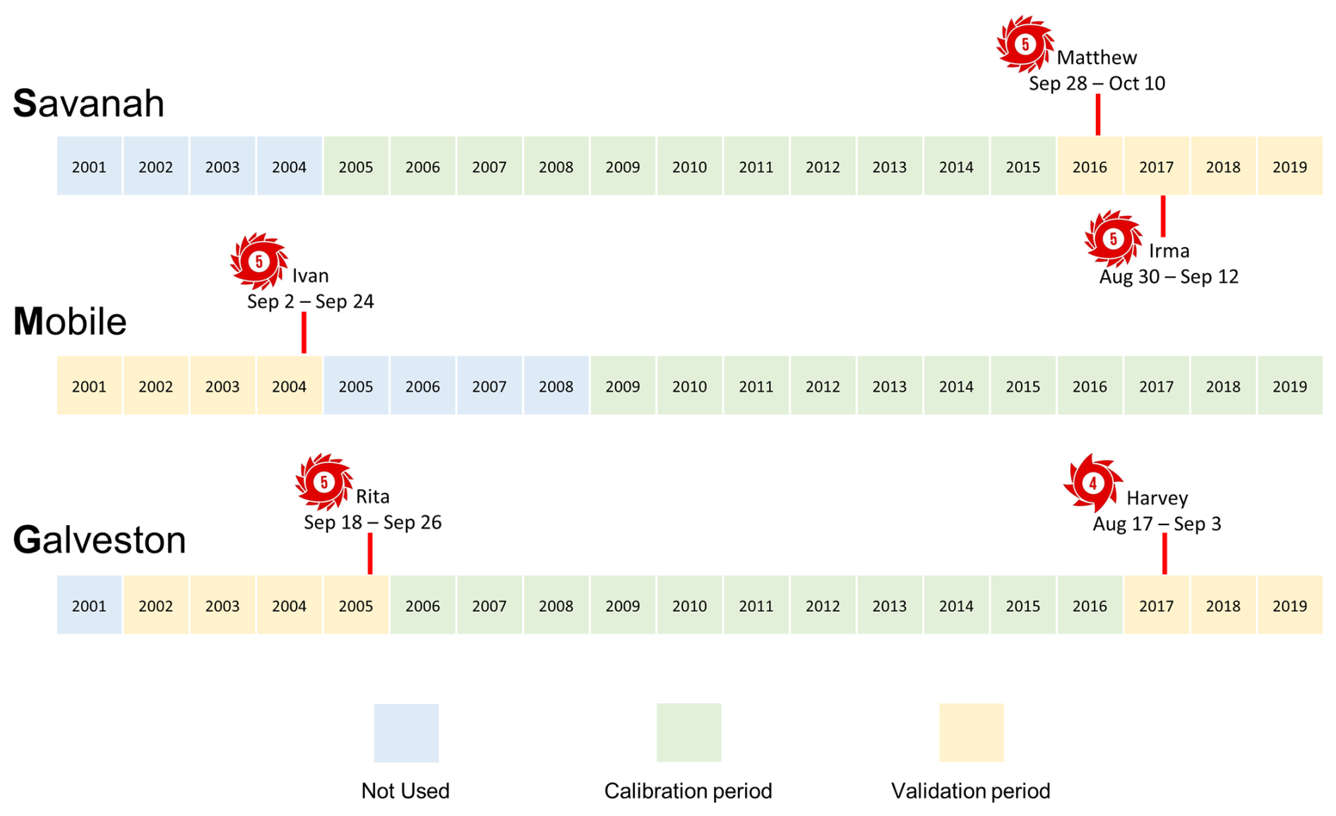
Figure 3 The calibration and validation periods considered in this study for three watersheds, along with the hurricane events and their respective durations.

The SAC-SMA model was calibrated separately for each drainage area associated with the USGS stations, rather than using the entire basin for the calibration process. This decision was based on the structure of the SAC-SMA model, which is a lumped model, meaning that it aggregates hydrological processes over a given area rather than considering them at individual sub-basins or locations. To ensure accurate representation of the hydrological processes, we calibrated and validated the model specifically at each USGS station while carefully accounting for the drainage area contributing to each station's flow. This is important for accurately calculating the model's forcing input variables – such as mean areal precipitation and mean areal potential evapotranspiration – since these inputs depend on the spatial extent of the drainage area for each station. By focusing on the specific drainage area for each USGS station, we ensure that the model's inputs reflect the local conditions of the watershed, leading to more reliable and representative model calibration and validation results. This method also improves the model's ability to simulate hydrological processes at the station level while considering the variations in environmental factors across different parts of the basin.

To ensure reliable initial conditions for the model's state variables, a 3-month spin-up period was used at the beginning of both the calibration and the validation periods. This warm-up period allowed the model to stabilize prior to the actual calibration and validation processes. The model state variables are those listed in Table 2 of our previous paper (Abbaszadeh et al., 2018).

3 Results and discussions

This study aims to account for all sources of uncertainties involved in hydrologic model predictions and their impact on improving hurricane-induced extreme river discharges across different regions in the SEUS. This section summarizes the performance of the SAC-SMA hydrologic model during both the calibration and the validation periods. It then explains the data assimilation settings along with the streamflow simulation capability of the SAC-SMA model with and without data assimilation. The study is conducted in multiple locations across three watersheds in the SEUS during hurricane events.

3.1 SAC-SMA model calibration and validation

Figure 4 illustrates the performance of the SAC-SMA model during both the calibration and the validation periods across all study regions utilized in this research. As previously mentioned, for parameter calibration of the SAC-SMA model, we utilized 10 years of historical USGS streamflow observation data, while model validation was conducted over a 4-year period encompassing flooding from various hurricane events (as shown in Fig. 3). Within this figure, the correlation coefficient (R), bias, and root mean square error (RMSE) represent the statistical measures of the relationship between simulated and observed streamflow values. We remind the reader that in this study, we run the hydrologic model over the USGS locations that have not been affected by the backwater effect of the downstream flow, and the streamflow observations have always been positive. These USGS locations are shown in Fig. 1 with black dots. The results confirm that although the SAC-SMA model was calibrated over the periods for which the river networks within the watersheds have not experienced flow as much as the validation periods, the model parameters were properly calibrated to simulate the streamflow. The model parameters are those listed in Table 1 of our previous paper (Abbaszadeh et al., 2018). The temporal resolution of streamflow simulation is daily. DA occurs at a daily timescale to match the output frequency of the SAC-SMA model. This strategy aims to minimize the impact of instantaneous streamflow changes on parameter updates during the assimilation process. While assimilating streamflow at sub-daily intervals could be advantageous for adjusting model state variables such as soil moisture storage, it is not anticipated to significantly contribute to updating model parameters, which typically vary at coarser timescales.

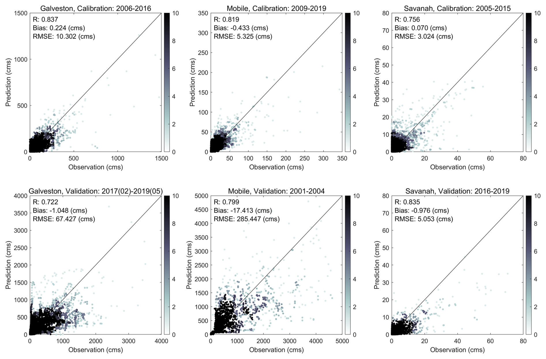
Figure 4 The performance of the SAC-SMA model during the calibration and validation periods over three watersheds in the southeastern US.

Figure 5 SAC-SMA model performance over the validation period across the USGS stations within the Galveston Watershed. RMSE unit is m³ s⁻¹.

Figure 5 illustrates the model performance (i.e., correlation coefficient and RMSE) across the USGS stations within the Galveston Watershed. Figure S1 in the Supplement shows the same results for the other two watersheds, Mobile and Savanah. The results for the Galveston Watershed show that the calibrated SAC-SMA model accurately simulates the streamflow across almost the entire region except the two USGS stations located downstream of Lake Livingston Dam. The primary function of this dam is flood control. Further analysis revealed that the lower performance of the model at these locations is attributed to the heavy rainfall of Hurricane Harvey that forced the Trinity River authority to release a record 3131.4 m³ s⁻¹ (110 600 ft³ s⁻¹) from Lake Livingston Dam (The Seattle Times, 2021), which resulted in a significant increase in the river flow. A similar event happened in the case of Hurricane Rita, which led to a significant flow increase in the Trinity River and severe flooding (TPWD, 2021). Although the SAC-SMA hydrologic model successfully simulated river flow across all USGS stations within the Galveston Watershed, it could not provide reliable streamflow simulation along the Trinity River due to the water release from Lake Livingston Dam during hurricanes Rita and Harvey. For the Mobile Watershed, as shown in Fig. S1, there is good agreement between the simulated and observed river discharge values across all USGS stations except station no. 02428400. Further investigations revealed that the river discharge at this location is computed based on flow through Claiborne Dam (for more information, see USGS, 2021b). During Hurricane Ivan, the flow at this USGS station reached more than 2800 m³ s⁻¹, probably due to water release from Claiborne Dam that consequently resulted in higher downstream river discharge.

Figure 6 NSE values for the USGS stations across the Galveston and Mobile watersheds. This result is based on the validation period.

The NSE values for the calibration period were 0.80, 0.78, and 0.69 for Galveston, Mobile, and Savanah, respectively. Similarly, for the validation period, the NSE values for these regions were 0.68, 0.71, and 0.65, respectively. Figure 6 also illustrates the NSE for the USGS stations across the Galveston and Mobile watersheds. In this figure, positive NSE values are shown with black circles, and negative NSE values are shown with red circles. The regulated USGS stations are marked with black dots to facilitate interpretation of model performance at those specific locations. The results indicate that, in general, the model performance is lower at the regulated USGS stations. For example, the NSE for USGS station 8074000 (Fig. 6) is negative; this station is located downstream of Addicks and Barker dams.

3.2 Improving streamflow forecasting using data assimilation

The primary goal of this research is to employ a data assimilation technique to account for all sources of uncertainty in the SAC-SMA model simulation and provide a more accurate and reliable streamflow prediction. The data assimilation approach used in this study was recently developed by the authors of this study and is used here for the first time to predict streamflow values during multiple hurricane events with heavy rainfall across different locations in the SEUS. As previously stated, the primary objective of our study is to assess the degree to which the developed data assimilation technique improves the prediction of extreme river flow caused by hurricanes. This section summarizes the performance of the SAC-SMA model after using the data assimilation. The meteorological forcing data, including precipitation and PET, are assumed to have log-normal and normal error distributions, with a relative error of 25 % in the DA setting (DeChant and Moradkhani, 2012). This assumption ensures that the meteorological observations' errors due to spatial heterogeneity inherent in these variables and sensor errors are accounted for. The model error is assumed to follow a normal distribution with a relative error of 25 %. Unlike the other data assimilation techniques, HEAVEN enables us to characterize, quantify, and take into account the model structural uncertainty using an explicit form of the model error covariance matrix within the data assimilation process. This feature of our developed data assimilation method is specifically more important in this study as we simulate the peak streamflow during hurricane events. As discussed in our previous paper (Abbaszadeh et al., 2019), in this data assimilation technique, the background error covariance matrix B gets adaptively inflated when the model attempts to simulate extreme values. This error covariance matrix inflation not only helps the 4D-Var objective function to find the optimal initial condition within the assimilation window (Cheng et al., 2019; Liu et al., 2008; Trémolet, 2007), but also ensures the exploration of a larger feasible solution space when the model states are being corrected within the particle filtering process, which results in a more complete representation of posterior distributions. In summary, the capability of the developed hydrologic data assimilation method to estimate peak flows stems from its automatic process of inflating and deflating the background error covariance matrix. This process enables the model to achieve a more realistic ensemble spread, leading to a more accurate expected value compared to the observed value.

Figure 7 Streamflow forecast improved by data assimilation during peak flow conditions across the USGS stations within all three watersheds. The values shown for the Savanah and Mobile stations are POI.

Here, we report the performance measures (i.e., correlation coefficient and RMSE) based on an ensemble size of 100 for 1 d ahead streamflow forecasting. Figures S2 and S3 show the model performance after using data assimilation across all USGS stations located within the study regions. It should be noted that these results are based on an ensemble size of 100, but of course, larger ensemble sizes would have resulted in better posterior estimates and more accurate and reliable streamflow forecasts. We realized that while data assimilation improved the SAC-SMA model performance across the majority of stations, in some locations the results remained suboptimal. Further investigation revealed that these are the same locations previously identified as being heavily influenced by upstream dam water release during hurricane events. These locations can not be used as upstream boundary conditions for hydrodynamic modeling (which is part of our future study), as they were heavily influenced by water release policy during the hurricane events, which altered the natural flow of the river, conditions under which hydrologic models most often fail to perform. Figure 7 depicts how data assimilation improved streamflow forecasting during peak flow conditions across USGS stations in the Galveston Watershed during Hurricane Harvey. Figure 7 shows the results for other watersheds and hurricane events, including Galveston–Rita, Mobile–Ivan, Savanah–Matthew, and Savanah–Irma. In Fig. 7, POI represents the percentage of improvement achieved by performing the assimilation. In other words, it shows how much the streamflow forecast improved (in percentage) by using data assimilation compared to using the open-loop model simulation (without assimilation). The findings revealed that, while data assimilation improved the SAC-SMA streamflow forecasting skill across almost all USGS station networks on the peak flow day of Hurricane Harvey, its contribution to improving streamflow forecasting during Hurricane Rita was marginal. Unlike Hurricane Harvey, where streamflow reached a peak gradually over the course of a few days (USGS, 2021a), in the case of Hurricane Rita, streamflow jumped from less than 28 m³ s⁻¹ (23 September) to more than 566 m³ s⁻¹ (24 September) in a single day (according to station no. 08066500, Trinity Rv at Romayor, Texas), such that the hydrologic model failed to detect the unexpected high flow on 24 September despite accurate initialization on 23 September (USGS, 2021b).

For hurricanes Ivan and Matthew in Mobile and Savanah, the percentage of improvement in the SAC-SMA model peak flow forecasts with data assimilation ranged from 21 % to 46 % and 5 % to 46 %, respectively, depending on the location of the USGS stations. Understanding and explicitly quantifying the degree to which each source of uncertainty, i.e., meteorological forcing, model parameters, initial condition, model structure, and parameterization, affects the final hydrologic model outputs are not feasible, as they are all connected and collectively contribute to degrading model performance. Our developed data assimilation technique, HEAVEN, has an explicit form of covariance error matrix for each source of uncertainty that feeds each other during the assimilation process, representing the interaction between different sources of uncertainties involved in different layers of model simulations. This results in a better representation of posterior distribution and reduction in uncertainty in hydrologic modeling. For this reason, we see that the data assimilation approach used in this study is an effective technique for improving streamflow forecasting skill during hurricane events.

Figure 8 The 1 d ahead streamflow forecast with and without data assimilation across multiple USGS stations in the Galveston Watershed in Texas during Hurricane Harvey. The green band represents the time window that contains the peak flow value.

Figure 8 illustrates the ensemble streamflow forecasts with and without data assimilation across multiple USGS stations in the Galveston Watershed. As seen in this figure, in all locations the ensemble mean is much closer to the observations compared to the streamflow mean value from the open-loop stimulation. The shaded blue area represents the 95 % uncertainty interval. We also see that in all cases the observations fall within the uncertainty interval. Therefore, we can conclude that using data assimilation, the hydrologic model results in more accurate and precise streamflow forecasts. In Fig. 8, the green band represents the time window that contains the peak flow value, not just the peak itself. This band is intended to show the broader period during which the peak flow occurs, rather than the single peak value. The verification process (POI reported in Fig. 7) was based on this entire time window, including the period before and after the peak.

4 Conclusions

This study investigates the application of the HEAVEN data assimilation technique to improve the forecasting of extreme river flow during hurricane-induced flooding in the SEUS. By integrating HEAVEN with the SAC-SMA hydrologic model, this research aimed to address the various sources of uncertainty in hydrologic simulations, particularly during extreme events such as hurricanes. The results show that HEAVEN effectively enhances the SAC-SMA model's streamflow forecasting capabilities by incorporating uncertainty from multiple sources, including meteorological forcing, model parameters, and structural errors.

The key findings highlight that data assimilation through HEAVEN significantly improved streamflow forecasts during peak flow conditions, especially in cases where extreme river discharge occurred. For example, in the Galveston Watershed during Hurricane Harvey, data assimilation led to substantial improvements in the forecasting of peak flows, with forecasted values being much closer to observed streamflow than those from the open-loop (non-assimilated) model. However, in cases like Hurricane Rita, where the streamflow increased abruptly within a very short time window, the assimilation approach was less effective. Despite accurate initial conditions, the model struggled to capture the rapid onset of extreme flow, highlighting a limitation of the current approach. This was due to the inability of the model to anticipate such a drastic shift in flow within a single day, an event that may require further refinement of the assimilation process to account for sudden, large fluctuations in discharge.

The HEAVEN technique proved to be capable of addressing model structural uncertainties by inflating and deflating the background error covariance matrix, ensuring a more reliable posterior distribution of streamflow forecasts. The assimilation process also facilitated the quantification and interaction of multiple sources of uncertainty, improving the overall robustness of the predictions. While the model performed well across most stations, some locations remained challenging, particularly those influenced by water releases from upstream dams. These locations, which significantly alter the natural flow dynamics, may require more specialized modeling approaches in future work, such as hydrodynamic modeling.

This study also discusses the computational limitations associated with optimizing the 4D-Var cost function using the Nelder–Mead algorithm, as tangent linear or adjoint models were not available. While this approach is effective, it remains computationally intensive. With the growing use of machine learning (ML) emulators in hydrologic modeling, future work may focus on incorporating these techniques to accelerate optimization and further enhance the efficiency of data assimilation in large-scale hydrologic forecasting.

In summary, the HEAVEN data assimilation method offers a promising advancement in the accurate prediction of extreme river flow during hurricane events, but challenges remain in addressing sudden and large fluctuations in streamflow. Future developments may focus on refining the assimilation process for such events and incorporating additional modeling techniques, such as hydrodynamic models for regulated river systems, to further improve forecasting accuracy and reliability.

Appendix A: EPFM

EPFM is a sequential data assimilation technique based on a combination of particle filtering, Markov chain Monte Carlo (MCMC), and the genetic algorithm (GA). EPFM is performed within the assimilation window for which the initial condition was obtained from the 4D-Var approach. Here we provide a brief overview of the EPFM algorithm. For more information, we refer readers to the original article (Abbaszadeh et al., 2018). Equations (A1) and (A2) describe the generic nonlinear dynamic system, where x_t∈Rⁿ and θ∈R^d are vectors of uncertain state variables and model parameters, respectively. Here, u_t represents the uncertain forcing data; y_t∈R^m indicates a vector of observation data; and ω_t and υ_t are the model and measurement errors, respectively, which are assumed to be independent and follow white noise with a mean of zero and covariance Q_t and R_t.

$$\begin{array}{}\text{(A1)}& {\displaystyle }{\mathit{x}}_{\mathrm{t}}=M(x_{t-\mathrm{1}},u_{\mathrm{t}},\mathit{\theta })+{\mathit{\omega }}_{\mathrm{t}}{\mathit{\omega }}_{\mathrm{t}}\sim N(\mathrm{0},Q_{\mathrm{t}})\text{(A2)}& {\displaystyle }{\mathit{y}}_{\mathrm{t}}=h\left({\mathit{x}}_{\mathrm{t}}\right)+{\mathit{\upsilon }}_{\mathrm{t}}{\mathit{\upsilon }}_{\mathrm{t}}\sim N(\mathrm{0},R_{\mathrm{t}})\end{array}$$

The following formula is used to calculate the posterior distribution of the state variables at time t:

$$\begin{array}{}\text{(A3)}& {\displaystyle }\begin{array}{rl}p\left({\mathit{x}}_{\mathrm{t}}\mathrm{|}{y}_{\mathrm{1}:t}\right)=& p({\mathit{x}}_{\mathrm{t}}\mathrm{|}{y}_{\mathrm{1}:t-\mathrm{1}},{\mathit{y}}_{\mathrm{t}})\\ =& {\displaystyle \frac{p\left({\mathit{y}}_{\mathrm{t}}\mathrm{|}{\mathit{x}}_{\mathrm{t}}\right)p\left({\mathit{x}}_{\mathrm{t}}\mathrm{|}{y}_{\mathrm{1}:t-\mathrm{1}}\right)}{p\left({\mathit{y}}_{\mathrm{t}}\mathrm{|}{y}_{\mathrm{1}:t-\mathrm{1}}\right)}}\\ =& {\displaystyle \frac{p\left({\mathit{y}}_{\mathrm{t}}\mathrm{|}{\mathit{x}}_{\mathrm{t}}\right)p\left({\mathit{x}}_{\mathrm{t}}\mathrm{|}{y}_{\mathrm{1}:t-\mathrm{1}}\right)}{\int p\left({\mathit{y}}_{\mathrm{t}}\mathrm{|}{\mathit{x}}_{\mathrm{t}}\right)p\left({\mathit{x}}_{\mathrm{t}}\mathrm{|}{y}_{\mathrm{1}:t-\mathrm{1}}\right)\mathrm{d}{\mathit{x}}_{\mathrm{t}}}},\end{array}\text{(A4)}& {\displaystyle }\begin{array}{rl}p\left({\mathit{x}}_{\mathrm{t}}\mathrm{|}{y}_{\mathrm{1}:t-\mathrm{1}}\right)& =\int p({\mathit{x}}_{\mathrm{t}},x_{t-\mathrm{1}}\mathrm{|}{y}_{\mathrm{1}:t-\mathrm{1}})\mathrm{d}{x}_{t-\mathrm{1}}\\ & =\int p\left({\mathit{x}}_{\mathrm{t}}\mathrm{|}{x}_{t-\mathrm{1}}\right)p\left(x_{t-\mathrm{1}}\mathrm{|}{y}_{\mathrm{1}:t-\mathrm{1}}\right)\mathrm{d}{x}_{t-\mathrm{1}},\end{array}\end{array}$$

where p(y_t|x_t) is the likelihood at time step t, $p\left({\mathit{x}}_{\mathrm{t}}\mathrm{|}{y}_{\mathrm{1}:t-\mathrm{1}}\right)$ is the prior distribution, and $p\left({\mathit{y}}_{\mathrm{t}}\mathrm{|}{y}_{\mathrm{1}:t-\mathrm{1}}\right)$ is the normalization factor. The marginal likelihood function p(y_1:t) and the normalization factor $p\left({\mathit{y}}_{\mathrm{t}}\mathrm{|}{y}_{\mathrm{1}:t-\mathrm{1}}\right)$ can be calculated using Eqs. (A5) and (A6), respectively.

$$\begin{array}{}\text{(A5)}& {\displaystyle }p\left(y_{\mathrm{1}:t}\right)=p\left(y_{\mathrm{1}}\right)\prod p\left({\mathit{y}}_{\mathrm{t}}\mathrm{|}{y}_{\mathrm{1}:t-\mathrm{1}}\right)\text{(A6)}& {\displaystyle }\begin{array}{rl}p\left({\mathit{y}}_{\mathrm{t}}\mathrm{|}{y}_{\mathrm{1}:t-\mathrm{1}}\right)& =\int p({\mathit{y}}_{\mathrm{t}},{\mathit{x}}_{\mathrm{t}}\mathrm{|}{y}_{\mathrm{1}:t-\mathrm{1}})\mathrm{d}{\mathit{x}}_{\mathrm{t}}\\ & =\int p\left({\mathit{y}}_{\mathrm{t}}\mathrm{|}{\mathit{x}}_{\mathrm{t}}\right)p\left({\mathit{x}}_{\mathrm{t}}\mathrm{|}{y}_{\mathrm{1}:t-\mathrm{1}}\right)\mathrm{d}{\mathit{x}}_{\mathrm{t}}\end{array}\end{array}$$

In hydrologic data assimilation using particle filtering, the posterior distribution is approximated by a set of particles, each with an associated weight:

$$\begin{array}{}\text{(A7)}& p\left({\mathit{x}}_{\mathrm{t}}\mathrm{|}{y}_{\mathrm{1}:t}\right)\approx \sum _{i=\mathrm{1}}^N{w}^{i+}\mathit{\delta }\left({\mathit{x}}_{\mathrm{t}}-{\mathit{x}}_{\mathrm{t}}^i\right),\end{array}$$

where wⁱ⁺, δ, and N denote the posterior weight of the ith particle, the Dirac delta function, and the ensemble size, respectively. The posterior weight is then normalized as follows:

$$\begin{array}{}\text{(A8)}& w^{i+}={\displaystyle \frac{w^{i-}\cdot p\left({\mathit{y}}_{\mathrm{t}}\mathrm{|}{\mathit{x}}_{\mathrm{t}}^i,{\mathit{\theta }}_{\mathrm{t}}^i\right)}{\sum _{i=\mathrm{1}}^N{w}^{i-}\cdot p\left({\mathit{y}}_{\mathrm{t}}\mathrm{|}{\mathit{x}}_{\mathrm{t}}^i,{\mathit{\theta }}_{\mathrm{t}}^i\right)}},\end{array}$$

where wⁱ⁻ is the prior particle weights, and $p({\mathit{y}}_{\mathrm{t}}\mathrm{|}{\mathit{x}}_{\mathrm{t}}^i,{\mathit{\theta }}_{\mathrm{t}}^i)$ can be computed from the likelihood $L({\mathit{y}}_{\mathrm{t}}\mathrm{|}{\mathit{x}}_{\mathrm{t}}^i,{\mathit{\theta }}_{\mathrm{t}}^i)$. To calculate this, for simplicity, a Gaussian likelihood is used as follows:

$$\begin{array}{}\text{(A9)}& \begin{array}{rl}L\left({\mathit{y}}_{\mathrm{t}}\mathrm{|}{\mathit{x}}_{\mathrm{t}}^i,{\mathit{\theta }}_{\mathrm{t}}^i\right)=& {\displaystyle \frac{\mathrm{1}}{\sqrt{(\mathrm{2}\mathit{\pi }{)}^{\mathrm{m}}\mathrm{|}{R}_{\mathrm{t}}\mathrm{|}}}}\exp [-{\displaystyle \frac{\mathrm{1}}{\mathrm{2}}}{\left({\mathit{y}}_{\mathrm{t}}-h\left({\mathit{x}}_{\mathrm{t}}^i\right)\right)}^{\mathrm{T}}\\ & \times R_{\mathrm{t}}^{-\mathrm{1}}\left({\mathit{y}}_{\mathrm{t}}-h\left({\mathit{x}}_{\mathrm{t}}^i\right)\right)].\end{array}\end{array}$$

In this data assimilation method, a GA evolutionary cycle is employed to shuffle the particles. The weights of the particles (wⁱ⁺) are treated as their fitness values. The particles (or population) are sorted in descending order of fitness, and the roulette wheel selection method is applied to choose parent particles for the crossover operation, generating offspring (new particles). The crossover probability determines the proportion of particles involved in the crossover process. To enhance the diversity of the offspring, a mutation operator is applied with a specified probability. For further details on the crossover and mutation operators and their respective equations, we refer readers to Abbaszadeh et al. (2018). Finally, the MCMC approach is used to either accept or reject the newly generated offspring particles (proposed state variables). This process requires re-running the model from t−1 to t using $x_{t-\mathrm{1}}^i$ (state variables before using GA operators) and $x_{t-\mathrm{1}}^{i,p}$ (state variables after using GA operators). To accept or reject the proposal states, the metropolis acceptance ratio α is calculated using Eq.  (A10).

$$\begin{array}{}\text{(A10)}& \begin{array}{rl}\mathit{\alpha }& =min\left(\mathrm{1},{\displaystyle \frac{p\left({\mathit{x}}_{\mathrm{t}}^{i,p},{\mathit{\theta }}_{\mathrm{t}}^{i-}\mathrm{|}{y}_{\mathrm{1}:t}\right)}{p\left({\mathit{x}}_{\mathrm{t}}^{i-},{\mathit{\theta }}_{\mathrm{t}}^{i-}\mathrm{|}{y}_{\mathrm{1}:t}\right)}}\right)\\ & =min\left(\mathrm{1},{\displaystyle \frac{p\left(y_{\mathrm{1}:t}\mathrm{|}{\mathit{x}}_{\mathrm{t}}^{i,p},{\mathit{\theta }}_{\mathrm{t}}^{i-}\right)\cdot p\left({\mathit{x}}_{\mathrm{t}}^{i,p}\mathrm{|}{\mathit{\theta }}_{\mathrm{t}}^{i-},y_{\mathrm{1}:t-\mathrm{1}}\right)}{p\left(y_{\mathrm{1}:t}\mathrm{|}{\mathit{x}}_{\mathrm{t}}^{i-},{\mathit{\theta }}_{\mathrm{t}}^{i-}\right)\cdot p\left({\mathit{x}}_{\mathrm{t}}^{i-}\mathrm{|}{\mathit{\theta }}_{\mathrm{t}}^{i-},y_{\mathrm{1}:t-\mathrm{1}}\right)}}\right),\end{array}\end{array}$$

where $p({\mathit{x}}_{\mathrm{t}}^{i,p},{\mathit{\theta }}_{\mathrm{t}}^{i-}\mathrm{|}{y}_{\mathrm{1}:t})$ is the proposed joint probability distribution.

$$\begin{array}{}\text{(A11)}& {\displaystyle }\begin{array}{rl}p\left({\mathit{x}}_{\mathrm{t}}^{i,p},{\mathit{\theta }}_{\mathrm{t}}^{i-}\mathrm{|}{y}_{\mathrm{1}:t}\right)& \propto p\left({\mathit{y}}_{\mathrm{t}}\mathrm{|}{\mathit{x}}_{\mathrm{t}}^{i,p},{\mathit{\theta }}_{\mathrm{t}}^{i-}\right)\\ & \times p\left({\mathit{x}}_{\mathrm{t}}^{i,p}\mathrm{|}{\mathit{\theta }}_{\mathrm{t}}^{i-},y_{\mathrm{1}:t-\mathrm{1}}\right)\\ & \times p\left({\mathit{\theta }}_{\mathrm{t}}^{i-}\mathrm{|}{y}_{\mathrm{1}:t-\mathrm{1}}\right)\end{array}\text{(A12)}& {\displaystyle }{\mathit{x}}_{\mathrm{t}}^{i,p}=M\left(x_{t-\mathrm{1}}^{i,p},u_{\mathrm{t}}^i,{\mathit{\theta }}_{\mathrm{t}}^{i-}\right)\end{array}$$

Here, $p({\mathit{y}}_{\mathrm{t}}\mathrm{|}{\mathit{x}}_{\mathrm{t}}^{i,p},{\mathit{\theta }}_{\mathrm{t}}^{i-})$ is computed using Eq. (A9), and the proposal state probability density function (PDF) $p({\mathit{x}}_{\mathrm{t}}^{i,p}\mathrm{|}{\mathit{\theta }}_{\mathrm{t}}^{i-},y_{\mathrm{1}:t-\mathrm{1}})$ is calculated with the assumption that it follows the marginal Gaussian distributions with mean μ_t (Eq. A14) and variance ${\mathit{\sigma }}_{\mathrm{t}}^{\mathrm{2}}$ (Eq. A15). To calculate the proposal PDF, the weighted mean and variance of the Gaussian distribution are calculated as follows:

$$\begin{array}{}\text{(A13)}& {\displaystyle }& {\displaystyle }{\mathit{x}}_{\mathrm{t}}^{i-}=M\left(x_{t-\mathrm{1}}^{i+},u_{\mathrm{t}}^i,{\mathit{\theta }}_{\mathrm{t}}^{i-}\right),\text{(A14)}& {\displaystyle }& {\displaystyle }{\mathit{\mu }}_{\mathrm{t}}=\sum w_{t-\mathrm{1}}^{i+}{\mathit{x}}_{\mathrm{t}}^{i-},\text{(A15)}& {\displaystyle }& {\displaystyle }{\mathit{\sigma }}_{\mathrm{t}}^{\mathrm{2}}=\sum w_{t-\mathrm{1}}^{i+}{\left({\mathit{x}}_{\mathrm{t}}^{i-}-{\mathit{\mu }}_{\mathrm{t}}\right)}^{\mathrm{2}}.\end{array}$$

Using the accepted proposal state variables, the posterior weights are recalculated using Eq. (A8), and these weights are then used to compute the effective sample size. The resampling step in the sequential data assimilation approach has been detailed in our previous work (Moradkhani et al., 2012), and we refer readers to that publication for further information.

Appendix B: How is variational data assimilation coupled with sequential data assimilation?

The Hybrid Ensemble and Variational Data Assimilation framework for Environmental Systems method combines EPFM with 4D-Var data assimilation. Its goal is to robustly estimate model states and parameters while accounting for structural, parameter, and input uncertainties in environmental systems. The hybrid framework leverages the sequential updating capability of EPFM and the batch optimization strengths of 4D-Var to address uncertainties at various stages of the modeling process. In this paper, we focus on how the prior (background) error covariance matrix B is updated during the sequential filtering process. This matrix is then used in the next assimilation cycle within the 4D-Var cost function. By applying Eq. (B1), we obtain the best estimates of the model state variables and parameters as the expected values of their posterior distributions at each time step within the assimilation window.

$$\begin{array}{}\text{(B1)}& {\displaystyle }\begin{array}{rl}{\stackrel{\mathrm{‾}}{x}}_k^{+}=& {\displaystyle \frac{\mathrm{1}}{N}}{\sum }_{i=\mathrm{1}}^N{x}_k^{i+}\text{ and }{\stackrel{\mathrm{‾}}{\mathit{\theta }}}_k^{+}={\displaystyle \frac{\mathrm{1}}{N}}{\sum }_{i=\mathrm{1}}^N{\mathit{\theta }}_k^{i+}\\ & \forall k=\mathrm{1},\mathrm{\dots },K\end{array}\text{(B2)}& {\displaystyle }{\mathit{\eta }}_k={\stackrel{\mathrm{‾}}{x}}_k^{+}-M_{k-\mathrm{1}\to k}\left({\stackrel{\mathrm{‾}}{x}}_{k-\mathrm{1}}^{+},{\stackrel{\mathrm{‾}}{\mathit{\theta }}}_k^{+},u_k\right)\text{(B3)}& {\displaystyle }q={\displaystyle \frac{\mathrm{1}}{K}}{\sum }_{k=\mathrm{1}}^K{\mathit{\eta }}_k\text{(B4)}& {\displaystyle }{\mathbf{B}}_{\mathrm{d}}={\displaystyle \frac{\mathrm{1}}{K-\mathrm{1}}}{\sum }_{k=\mathrm{1}}^K[{\mathit{\eta }}_k-q][{\mathit{\eta }}_k-q{]}^{\mathrm{T}}\text{(B5)}& {\displaystyle }{\mathbf{B}}_{\mathrm{s}}=\mathbf{B}\text{(B6)}& {\displaystyle }\mathbf{B}=(\mathit{\gamma }\times {\mathbf{B}}_{\mathrm{s}})+(\mathrm{1}-\mathit{\gamma })\times {\mathbf{B}}_{\mathrm{d}}\mathrm{0}\le \mathit{\gamma }\le \mathrm{1}\end{array}$$

Here, η_k and q represent the estimates of model error and model error bias at each time within the assimilation window. In this approach, the EPFM filter is applied within the assimilation window, where the best initial condition is estimated using the 4D-Var method. A key challenge arises regarding how to use the deterministic (single) initial condition obtained from 4D-Var to initialize the EPFM filter, which is an ensemble-based approach. To address this, we define a prior error covariance matrix B, consisting of two components – dynamic (B_d) and static (B_s) prior error covariances – to perturb the deterministic solution from the 4D-Var method and generate the best initial condition for the EPFM filter. The dynamic prior error covariance matrix B_d is introduced by Shaw and Daescu (2016) in the assimilation cycle, while B represents the prior error covariance matrix from the previous assimilation cycle. The static prior error covariance matrix B_s is used in the current assimilation cycle. The prior error covariance matrix B is updated using Eq. (B6). The tuning factor γ controls the contribution of model error within the current assimilation cycle.

Appendix C: The implementation process

1. Initialization

Three essential error covariance matrices are initialized. This section highlights how different sources of uncertainties are accounted for with the proposed approach.

• The prior error covariance (B) combines dynamic (B_d) and static (B_s) components:

  $\mathbf{B}=(\mathit{\gamma }\times {\mathbf{B}}_{\mathrm{s}})+(\mathrm{1}-\mathit{\gamma })\times {\mathbf{B}}_{\mathrm{d}}\mathrm{0}\le \mathit{\gamma }\le \mathrm{1}$.

• The observation error covariance (R_k) assumes observation errors are Gaussian:

  ${\mathbf{R}}_{\mathrm{k}}={\left(max\left(\right(\mathit{\lambda }\times y_k),\mathrm{1})\right)}^{\mathrm{2}},$(Eq. 2, Sect. 2.4)

  where λ is the observation error percentage.

• The model error covariance (Q_k) is initialized as

  ${\mathbf{Q}}_{\mathrm{k}}=\mathrm{\Gamma }\times \text{diag}\left((\mathit{\pi }\times x_{\mathrm{0},\mathrm{b}}{)}^{\mathrm{2}}\right),$(Eq. 4, Sect. 2.4)

  where π is the error percentage in the model structure, and Γ is an inflation or deflation factor.

• Parameters (Θ) and initial ensembles ($x_{\mathrm{0}}^i$) are generated using Latin hypercube sampling (LHS).

2. Variational initialization (Step 1)

A deterministic state estimation is performed using 4D-Var. This step minimizes the cost function that combines prior, observational, and model error contributions. To avoid the need for model linearization, derivative-free optimization methods like the Nelder–Mead algorithm are used to find optimal solutions. The 4D-Var method minimizes a cost function to estimate the optimal state x_a for the assimilation window [t₀t_k]. The cost function incorporates prior, observational, and model error terms.

• $J(x_{\mathrm{0}},\mathrm{\dots },x_K)=J^{\mathrm{b}}+J^{\mathrm{o}}+J^{\mathrm{q}}$

  The background term (J^b) penalizes deviations of the initial state x₀ from the background (or prior) state x_0,b. It is weighted by the inverse of the prior error covariance matrix B.

• $J^{\mathrm{b}}=\frac{\mathrm{1}}{\mathrm{2}}(x_{\mathrm{0}}-x_{\mathrm{0},\mathrm{b}}{)}^{\mathrm{T}}{\mathbf{B}}^{-\mathrm{1}}(x_{\mathrm{0}}-x_{\mathrm{0},\mathrm{b}})$

  The observation term (J^o) penalizes the difference between the model-predicted observations h(x_k) and the actual observations y_k over all time steps within the assimilation window.

• $\frac{\mathrm{1}}{\mathrm{2}}\sum _{k=\mathrm{0}}^K(y_k-h_k(x_k\left){)}^{\mathrm{T}}{\mathbf{R}}_{\mathrm{k}}^{-\mathrm{1}}\right(y_k-h_k\left(x_k\right))$

  The model error term (J^q) accounts for discrepancies between the model-predicted state at time k and the actual state x_k. It reflects the uncertainty in the model dynamics.

• $\frac{\mathrm{1}}{\mathrm{2}}\sum _{k=\mathrm{1}}^K(x_k-M_{k-\mathrm{1}\to k}(x_{k-\mathrm{1}},\mathrm{\Theta },u_k\left){)}^{\mathrm{T}}{Q}^{-\mathrm{1}}\right(x_k-M_{k-\mathrm{1}\to k}(x_{k-\mathrm{1}},\mathrm{\Theta },u_k))$

  Here, h(x_k) is the observation operator at time k, and $M_{k-\mathrm{1}\to k}$ is the model transition operator between k−1 and k.

  To avoid linearization of M and h, derivative-free optimization methods (e.g., Nelder–Mead) are employed.

3. Ensemble generation (Step 2)

The deterministic 4D-Var solution is perturbed using the prior error covariance matrix B, resulting in an initial ensemble of states for particle filtering. This step bridges the sequential and variational components. The deterministic 4D-Var solution x_a is perturbed using the prior error covariance matrix B to generate an ensemble:

• $x_{\mathrm{0}}^i=x_{\mathrm{a}}+{\mathit{\epsilon }}^i{\mathit{\epsilon }}^i\sim N(\mathrm{0},\mathbf{B}).$(Eq.  6, Sect. 2.4)

4. Sequential assimilation via EPFM (Step 3)

The EPFM filter updates states and parameters sequentially by approximating the posterior distribution p(x_t|y_1:t).

• $p\left({\mathit{x}}_{\mathrm{t}}\mathrm{|}{y}_{\mathrm{1}:t}\right)\propto p\left({\mathit{y}}_{\mathrm{t}}\mathrm{|}{\mathit{x}}_{\mathrm{t}}\right)p\left({\mathit{x}}_{\mathrm{t}}\mathrm{|}{y}_{\mathrm{1}:t-\mathrm{1}}\right)$

  Here, p(y_t|x_t) is the prior distribution, and $\left({\mathit{x}}_{\mathrm{t}}\mathrm{|}{y}_{\mathrm{1}:t-\mathrm{1}}\right)$ is the likelihood of observations.

The posterior is represented as a weighted ensemble:

• $p\left({\mathit{x}}_{\mathrm{t}}\mathrm{|}{y}_{\mathrm{1}:t}\right)\approx \sum _{i=\mathrm{1}}^N{w}^{i+}\mathit{\delta }\left({\mathit{x}}_{\mathrm{t}}-{\mathit{x}}_{\mathrm{t}}^i\right).$(Eq.  A7)

To avoid particle degeneracy, an evolutionary Monte Carlo approach combines GA with MCMC. The mutation and crossover steps in GA ensure particle diversity, while MCMC refines the posterior ensemble. See Appendix A for more information.

5. Updating error covariance matrices (Steps 4–5)

The dynamic error covariance matrix B_d is estimated using ensemble-based error propagation:

• ${\mathit{\eta }}_k={\stackrel{\mathrm{‾}}{x}}_k^{+}-M_{k-\mathrm{1}\to k}\left({\stackrel{\mathrm{‾}}{x}}_{k-\mathrm{1}}^{+},{\stackrel{\mathrm{‾}}{\mathit{\theta }}}_k^{+},u_k\right),$(Eq.  B2)

• $q=\frac{\mathrm{1}}{K}{\sum }_{k=\mathrm{1}}^K{\mathit{\eta }}_k,$(Eq.  B3)

• ${\mathbf{B}}_{\mathrm{d}}=\frac{\mathrm{1}}{K-\mathrm{1}}{\sum }_{k=\mathrm{1}}^K[{\mathit{\eta }}_k-q][{\mathit{\eta }}_k-q{]}^{\mathrm{T}}.$(Eq.  B4)

The prior error covariance B is updated as

• $\mathbf{B}=(\mathit{\gamma }\times {\mathbf{B}}_{\mathrm{s}})+(\mathrm{1}-\mathit{\gamma })\times {\mathbf{B}}_{\mathrm{d}}.$(Eq.  B6)

6. Iterative feedback loop

The updated BB and EPFM posterior states feed back into the 4D-Var method as prior conditions for the next assimilation cycle. This iterative exchange ensures consistent improvement of states and parameters over time.

Appendix D: Uncertainty handling in HEAVEN

HEAVEN explicitly handles uncertainties at multiple stages. Model structural uncertainty is incorporated through dynamic error covariance B_d and feedback loops. Parameter and forcing uncertainty is addressed via the EPFM ensemble framework. Observation uncertainty is modeled through R_k and integrated into the cost function. By combining sequential and variational approaches, HEAVEN offers a comprehensive solution for state and parameter estimation in nonlinear, uncertain systems. Steps where major uncertainties are addressed include generating the initial ensemble (Step 2), dynamically updating B (Step 5), and using ensemble posterior information in feedback loops (Step 6).