Skilful probabilistic predictions of UK flood risk months ahead using a large-sample machine learning model trained on multimodel ensemble climate forecasts

Seasonal streamflow forecasts are an important component of flood risk management. Hybrid forecasting methods that predict seasonal streamflow using machine learning (ML) models driven by climate model outputs are currently underexplored, yet they have some important advantages over traditional approaches using hydrological models. Here we develop a hybrid subseasonal to seasonal (S2S) streamflow forecasting system to predict the monthly maximum daily streamflow up to 4 months ahead. We train a quantile regression forest model on dynamical precipitation and temperature forecasts from a multimodel ensemble of 196 members (eight seasonal climate forecast models) from the Copernicus Climate Change Service (C3S) to produce probabilistic hindcasts for 579 stations across the UK for the period 2004–2016, with up to 4 months' lead time. We show that the large-sample (multi-site) ML model trained on pooled catchment data together with static catchment attributes is narrowly but significantly more skilful compared to single-site ML models trained on data from each catchment individually. Considering all initialisation months, 60 % of stations show positive skill (CRPSS > 0) relative to climatological reference forecasts in the first month after initialisation. This falls to 41 % in the second month, 38 % in the third month, and 33 % in the fourth month.

1 Introduction

Reliable streamflow forecasts weeks to months ahead are vital for managing the impacts of hydrological variability and extremes. Dynamical subseasonal to seasonal (S2S) streamflow forecasts are commonly produced by forcing a conceptual or physics-based hydrological model with the outputs of dynamical seasonal forecasts from climate models and may also include a subsequent statistical or machine learning (ML) post-processing step. This may be achieved either directly or indirectly, e.g. by using dynamical climate prediction information as direct inputs to the hydrological model or by using the dynamic predictions or empirical information as conditioning factors in a statistical weather generation scheme to create the model's input meteorological forecasts. These systems represent the current standard in S2S streamflow forecasting, underpinning flood forecasting services in Europe (Arheimer et al., 2020; Arnal et al., 2018), the USA (Demargne et al., 2014), Australia (Bennett et al., 2017), and globally (Emerton et al., 2018).

The chaotic nature of the atmosphere places a time limit of around 14 d on the predictability of weather from initial atmospheric circulation conditions, although this limit may vary from less than 1 week to nearly 3 weeks depending on local climate features and the current weather regime. S2S hydrometeorological forecasts therefore rely on relatively slowly varying aspects of the climate system that are more predictable beyond weather timescales, including initial hydrometeorological conditions and large-scale climate variability modes (Doblas-Reyes et al., 2013; Emerton et al., 2018). While the skill of seasonal climate forecasts is relatively low in the extra-tropics compared to other parts of the world (Doblas-Reyes et al., 2013), recent progress in forecasting European climate has resulted in skilful seasonal climate forecasts that support various climate services (e.g. Arheimer et al., 2020). For example, the European Flood Awareness System (EFAS) is at the forefront of operational streamflow forecasting in Europe, providing a pan-European service that aims to support preparatory action before major floods. The seasonal component of EFAS uses precipitation, temperature, and evaporation from the ECMWF seasonal prediction system (SEAS5) to drive LISFLOOD, a physics-based distributed hydrological model that estimates hydrological states and fluxes with a daily time step (Arnal et al., 2018). Operationally, EFAS produces seasonal streamflow outlooks for Europe at the beginning of each month up to 7 months ahead. Previous work using this setup suggests that skilful forecasts may be obtained for lead times up to 1 month ahead but that skill decreases gradually thereafter (Arnal et al., 2018).

The conceptual and physics-based hydrological models used operationally are computationally intensive relative to data-driven (statistical, empirical, machine learning) approaches. Spatial downscaling and bias correction of meteorological forecasts are needed to bridge the gap between the relatively coarse spatial scale of S2S climate prediction systems and the finer-resolution inputs needed by hydrological models, introducing a layer of methodological uncertainty to the process-based seasonal hydrologic forecasting process. The hydrological forecast outputs may then require further bias correction before they can be used (Yuan et al., 2015). In contrast, hybrid methods for seasonal streamflow forecasting overcome many of the shortcomings of dynamical approaches (Slater et al., 2023). Instead of using the downscaled outputs of dynamical seasonal prediction systems to drive a hydrological model, hybrid methods use dynamical climate predictions to drive statistical or machine learning models to directly predict the target variables of interest, e.g. streamflow quantiles or flood frequency. The dynamical climate predictions provide valuable information on large-scale climate patterns and atmospheric conditions, while the statistical or machine learning models offer the ability to capture complex nonlinear relationships related to streamflow behaviour. Such hybrid approaches follow from similar concepts used in empirical S2S hydrologic prediction, in which observed climate system variables, reanalyses, or indices (but not dynamical climate forecasts) are used in statistical schemes to predict streamflow directly (e.g. Mendoza et al., 2017; Regonda et al., 2006).

By combining the strengths of both dynamical and statistical approaches, hybrid methods have shown promise for improving seasonal streamflow predictions. For example, Tian et al. (2022) developed a hybrid framework that skilfully predicted month-ahead reservoir inflows in two US watersheds (in Colorado and Alabama) using an ML model driven by seasonal climate forecasts, along with observed large-scale climate indices and satellite-based estimates of antecedent conditions. In Europe, Hauswirth et al. (2023) showed that a single-site hybrid seasonal forecasting system could skilfully predict surface water level up to 3 months ahead using ML models driven by climate and hydrological inputs from SEAS5. Hybrid methods are unconstrained by the need to conserve the water balance and can implicitly handle biases in the climate data (Slater et al., 2023). Furthermore, they are able to exploit relationships between variables at different spatial and temporal resolutions and spatial extents, e.g. relating daily local streamflow quantiles to monthly climate inputs or large-scale climate patterns (Moulds et al., 2023; Tian et al., 2022).

Previous work using observed data for hydrological simulation has shown that ML models work best when trained on data from multiple catchments (Nearing et al., 2021). While much of the recent literature on this topic focuses on deep learning architectures (e.g. Kratzert et al., 2019), similar results have been found for tree-based models (e.g. Gauch et al., 2021). Large-sample (or multi-site) approaches allow the models to learn relationships from a large envelope of hydrological variability that encompasses a broad spectrum of catchment characteristics, which they can use effectively to make predictions in individual catchments (e.g. Lees et al., 2021, 2022). However, the potential added value of a large-sample approach has not yet been evaluated for seasonal flood prediction using ML models trained on climate forecasts. Addressing this gap is necessary because seasonal climate forecasts are typically highly uncertain, at levels of skill near a minimal threshold of uncertainty. The sample size of available records for training hydrological forecast models is much smaller at subseasonal to seasonal scales than at short- to medium-range scales. Thus, new methods that pool forecasts over both space and time may be a promising strategy to extract greater forecast signal from small-sample noise.

Here we develop and test a hybrid forecasting system to predict the monthly maximum daily flow values (Q_max) at lead times of up to 4 months for 579 catchments in the UK. The maximum probable flow in each month is an indicator of flood risk, though it does not predict the exact timing or volume of a future flood event. We train a large-sample machine learning model to predict Q_max using seasonal forecasts of precipitation and temperature from the Copernicus Climate Change Service (C3S) multimodel ensemble alongside antecedent conditions and catchment characteristics. We focus on the monthly maximum daily streamflow rather than other common S2S hydrologic predictands (such as monthly or seasonal average flow) because it serves as an indicator of future flood hazards at S2S lead times while also presenting a significant challenge, as individual flood events (timing and magnitude) cannot be skilfully predicted beyond weather timescales. We address two main research questions: (i) how skilfully can the monthly maximum daily flow be predicted several months ahead using uncorrected monthly dynamical climate forecasts and antecedent conditions? (ii) To what extent can the skill of S2S streamflow predictions be improved at individual sites by developing a large-sample machine learning model that leverages static catchment attributes from a large collection of catchments to learn the hydrological behaviour at individual sites?

2 Materials and methods

2.1 Data

2.1.1 Streamflow

For the prediction target and observational validation dataset, we used daily streamflow observations for Great Britain from the National River Flow Archive (NRFA, 2023). We first selected stations that had streamflow records between 1994 and 2016 to match the hindcast period of the climate models, before discarding stations with less than 95 % data availability in any given year. We also discarded any stations that were not included in the CAMELS-GB dataset (Coxon et al., 2020), leaving a total of 579 stations. We computed specific discharge (mm d⁻¹) by dividing the daily streamflow values by the catchment area, then calculated the monthly maximum daily specific discharge for all months and stations.

2.1.2 Climate (re)forecasts

Monthly predictions of precipitation and temperature were obtained from the Copernicus Climate Change (C3S) multimodel seasonal forecasting system. We took seasonal reforecasts (“hindcasts”) of precipitation and temperature for the period 1994–2016 from eight seasonal prediction systems, resulting in a large multimodel ensemble of 196 members (Table S1). We computed the multimodel ensemble mean values of precipitation and temperature. We found that including quantiles (0.05, 0.25, 0.5, 0.75, 0.95) drawn from the precipitation and temperature ensemble as additional covariates alongside the mean values in the ML models did not improve skill (results not shown). We computed the climate inputs for each catchment by taking the area-weighted average monthly value for each variable. All C3S forecasting systems are assigned a nominal start date of the first day of each month such that no members are initialised using observations later than this date, although the initialisation method varies across the individual systems. Hereafter we refer to the predictions for the month immediately following initialisation as having a lead time of zero (e.g. for a forecast initialised on 1 August, the zeroth lead time prediction covers 1–31 August). The C3S forecasting system predicts climate up to a minimum of 6 months ahead, but we focus on the first 4 months following initialisation, as we are unlikely to observe substantial skill for monthly predictands thereafter (e.g. Arnal et al., 2018; Harrigan et al., 2018).

2.1.3 Antecedent catchment conditions

We used antecedent mean monthly streamflow as a proxy indicator of initial catchment soil moisture conditions, an important driver of seasonal hydrologic predictability (Arnal et al., 2018; Bierkens and Van Beek, 2009). We used the monthly mean specific discharge in the 3 months prior to the forecast initialisation to create three predictor variables describing the mean specific discharge over 1 month, 2 months, and 3 months prior to the nominal forecast initialisation date. We also included estimates of antecedent precipitation using ERA5 reanalysis data, creating variables to represent the average precipitation over 1 month, 2 months, and 3 months prior to the initialisation time. Antecedent precipitation and streamflow are both employed as proxies for hydrologic initial conditions and are likely to exhibit some degree of collinearity. However, as random forests are relatively robust to multicollinearity, we chose to retain both predictors in the model.

2.1.4 Catchment attributes

Large-sample ML models trained on data from hundreds of stream gauges simultaneously can benefit from additional information about spatial variability in catchment characteristics relative to single-site models (e.g. Lees et al., 2021; Slater et al., 2024). Here we included static catchment descriptors from the CAMELS-GB dataset (Table S3; Coxon et al., 2020) in our ML model. We also tried including streamflow signatures that describe the hydrologic behaviour of each catchment, including the baseflow index, the slope of the flow duration curve, the 5th and 95th percentiles of daily streamflow, and the mean daily streamflow. These were computed using data up to the start of the test period (2004) of our hybrid models to prevent data leakage (i.e. the situation where a statistical or ML model is inadvertently trained on the same data it will later be tested on). However, although the signature predictors assumed high importance in the quantile regression forests (QRF) model, they did not increase the Q_max forecasting skill, suggesting that the model can learn these hydrological characteristics from the static catchment attributes alone. We therefore left out the streamflow signatures from the final multi-site model.

2.2 Methods

We predict the monthly maximum daily streamflow (Q_max) using both dynamic and static predictor variables. Most large-sample ML approaches for hydrologic prediction employ long short-term memory (LSTM) models, which are well suited for sequential modelling at daily time steps. However, in this study, we employ quantile regression forests (QRF; Meinshausen, 2006), a nonparametric ensemble method that is well suited for working with single monthly aggregated forecasts from C3S. QRF models extend traditional random forests (Breiman, 2001) by estimating conditional quantiles of the response variable, enabling probabilistic predictions. Like random forests, QRF models are adept at exploiting nonlinear relationships between dependent and independent variables and require relatively little tuning because their performance is less sensitive to the values of hyperparameters compared to many other ML methods (Tyralis et al., 2019). QRF models can also be interrogated to establish the relative importance of predictor variables.

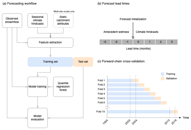
Figure 1 Key features of the forecast system. (a) Overview of steps in the forecasting workflow. (b) Forecast lead times used in the study. A separate model is trained for each lead time to account for changing climate model biases. (c) Schematic of the forward-chain cross-validation procedure employed during model training.

2.2.1 Model training

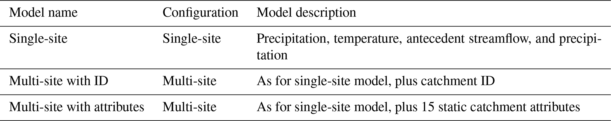
We train the model directly on the dynamical S2S forecast outputs to avoid introducing additional uncertainty due to post-processing (Fig. 1a). Like other forms of regression, the ML model implicitly performs bias correction by relating the raw climate inputs to observed streamflow (e.g. Slater et al., 2023; Slater and Villarini, 2018). We compared three model structures to predict Q_max in each catchment (Table 1). Firstly, we trained QRF models on each streamflow time series independently, giving a site-specific model for every catchment. We compared the single-site models with a multi-site QRF model that was trained on all (n=579) available streamflow time series data at once. To assess the extent to which the multi-site model learns from catchment attributes, we also include a multi-site model with the catchment ID as the only static attribute. Owing to the inherent robustness of QRF to potentially irrelevant predictors, whereby unimportant features are automatically downweighted, we do not perform predictor variable selection or screening.

Table 1 Formulation of the three ML models used in the analysis. Precipitation and temperature are the monthly ensemble mean values from the C3S multimodel system. Antecedent precipitation is the forecasted precipitation from the month prior to the target month, with lead times varying between 1 and 3 months (i.e. to make a prediction in lead time 4, the antecedent precipitation would be taken from lead time 3). Antecedent streamflow is the mean daily observed streamflow prior to the forecast initialisation. Catchment attributes are listed in Table S1.

In both single-site and multi-site approaches, a separate QRF model is trained for each lead time using all months from the training period. This is because the biases in the climate forecasts often change over time from initialisation, so a model trained on climate forecasts with a lead time of 1 month would be unsuitable to make predictions using climate forecasts with a lead time of 2 months. We note that a similar approach is used for bias-correcting seasonal climate forecasts (Crochemore et al., 2016). Another possibility would be to train a model on all lead times at once, with the lead time itself included as a categorical variable. We tried this but found that it degraded predictive skill. Thus, for each training period we obtain four models, trained on climate predictions with lead times of 1, 2, 3, and 4 months ahead, respectively (Fig. 1b). Dataset stratification choices are important in S2S prediction because predictability and prediction system biases typically vary seasonally and with lead time. There are strong geophysical reasons to tailor a statistical or empirical model using both factors, but each stratification dimension reduces the sample size available for training and testing; thus a trade-off is often adopted (e.g. Lehner et al., 2017). Here we do not stratify by initialisation date (i.e. month). We construct an ensemble forecast by using the QRF model to predict the conditional quantiles of Q_max corresponding to probabilities between 0.01 and 0.99, with an interval of 0.02.

We use a forward-chain cross-validation approach whereby the models are trained on reforecasts from the previous n years and tested on the current year (Fig. 1c). For example, to predict all months in 2004, the first training period was taken as January 1994 to December 2003. For 2005, we then extended the training period by 1 year to December 2004, and we continued adding 1 year until 2016, the final year in the test period, at which point the training period for the QRF models was January 1994 to December 2015. The climate predictors consisted of the multimodel ensemble mean of monthly precipitation and temperature (Table S1). We did not include a separate validation dataset (i.e. in a train/validate/test framework) because we found there was limited benefit to be gained from tuning the hyperparameters of the QRF model. The forward-chain cross-validation approach means that the model was retrained each year using data up to the previous year. The overall test results combine the test results for the individual years. This ensures the model is never tested on data it has been exposed to during training.

2.2.2 Forecast evaluation

We evaluated predictive skill using the continuous ranked probability score (CRPS) and associated skill score (CRPSS), common metrics for ensemble forecast evaluation. The CRPS represents the error between the forecast and observed cumulative distribution functions (Wilks, 2019). It ranges between zero and positive infinity and is negatively oriented (i.e. smaller values are better), similar in concept to other common error terms (e.g. mean absolute error). We evaluated our forecasts against an observation-based ensemble climatological forecast consisting of the observed monthly maximum daily streamflow values from the previous 20 years (e.g. Hauswirth et al., 2023), along with EFAS seasonal hindcasts. We used the CRPSS to evaluate the probabilistic skill of our ML forecasts relative to the reference ensemble climatology. The CRPSS ranges between negative infinity and 1, where 1 indicates perfect skill and 0 or below indicates no skill compared to the reference forecast. We computed the CRPS of the forecast and reference for each month in the test period (2004–2016) and took the mean across individual months to compute the CRPSS.

We complemented the CRPS (CRPSS) with the anomaly correlation coefficient (ACC) and reliability index (RI) (Renard et al., 2010). The ACC varies between −1 and 1, with a score of 1 representing perfect correlation between observed and forecast streamflow values. The RI is a probabilistic measure of the extent to which the forecast ensemble spread represents the uncertainty in observations. It varies between 0 and 1, with 1 denoting a perfectly reliable forecast. Like the CRPSS, we calculate the ACC and RI for every month and lead time separately. Lastly, we assessed the relative importance of the predictor variables using the Gini index, which measures the importance of individual variables in tree-based ML models. Specifically, the Gini index quantifies the extent to which a variable contributes to making homogeneous groups, where outcomes are similar and predictions are more reliable, while reducing impurity, indicating mixed groups with less predictable outcomes.

3 Results

The multi-site model with catchment attributes significantly outperforms the multi-site model with the catchment ID alone (Fig. 2a). This suggests that including static catchment attributes enables the model to better reproduce the hydrologic behaviour of different catchments, aligning with previous research for the UK on ML applied to daily streamflow simulation using observed climate inputs (e.g. Lees et al., 2021, 2022) and with findings on the performance of ML models for prediction in ungauged basins (Kratzert et al., 2019). Considering the skill scores for each lead time and combining all initialisation months, the multi-site model with catchment attributes narrowly but significantly outperforms the single-site models at lead times of 1 to 3 months, with a similar average performance between the multi-site and single-site model for the zeroth lead time (Fig. 2b). However, the relative performance of the multi-site model with attributes and the single-site model varies by forecast month and lead time (Fig. 3). For the zeroth lead time, the multi-site model tends to outperform the single-site model in the months where the highest skill is observed (i.e. December, January, June, July).

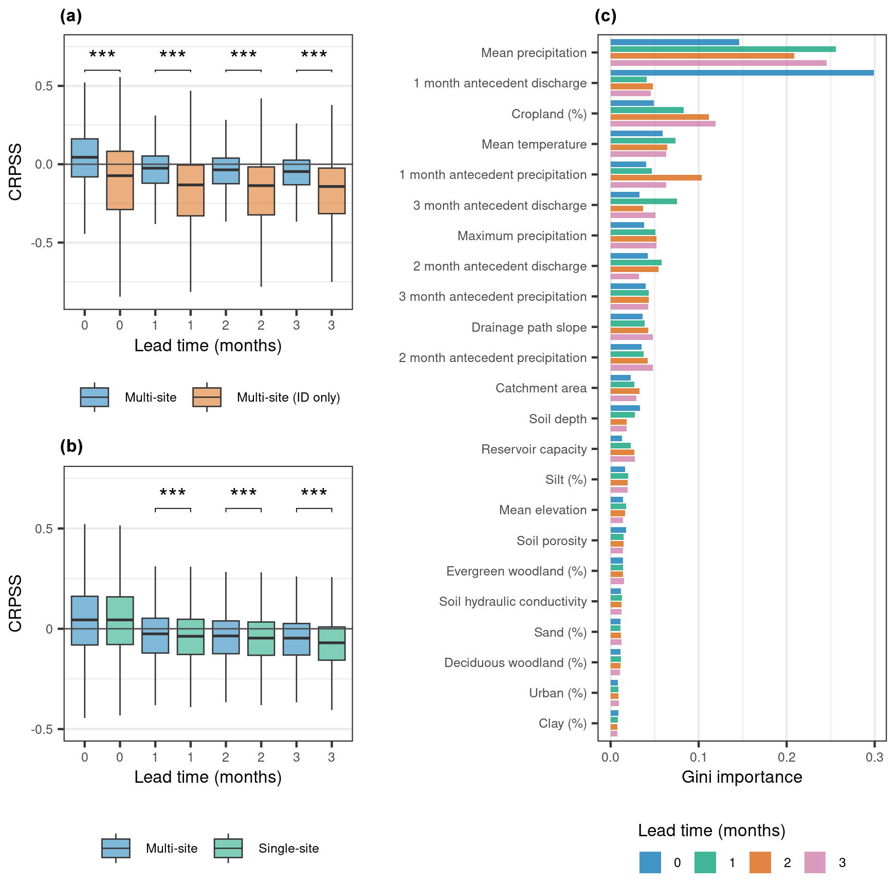
Figure 2 Analysis of model performance. (a) Comparison of the CRPSS for all months for multi-site models with catchment attributes and with the catchment ID only. We used a two-sided Wilcoxon signed-rank test to assess whether differences in skill scores between the models were significant (${}^{***}=p\mathit{<}\mathrm{0.001}$, ${}^{**}=p\mathit{<}\mathrm{0.01}$, ${}^{*}=p\mathit{<}\mathrm{0.05}$). (b) Comparison of the single-site model and the multi-site model with catchment attributes. (c) Relative importance of predictor variables in the multi-site model with catchment attributes for each lead time. Time-varying predictors are marked with an asterisk (e.g. ^* mean precipitation).

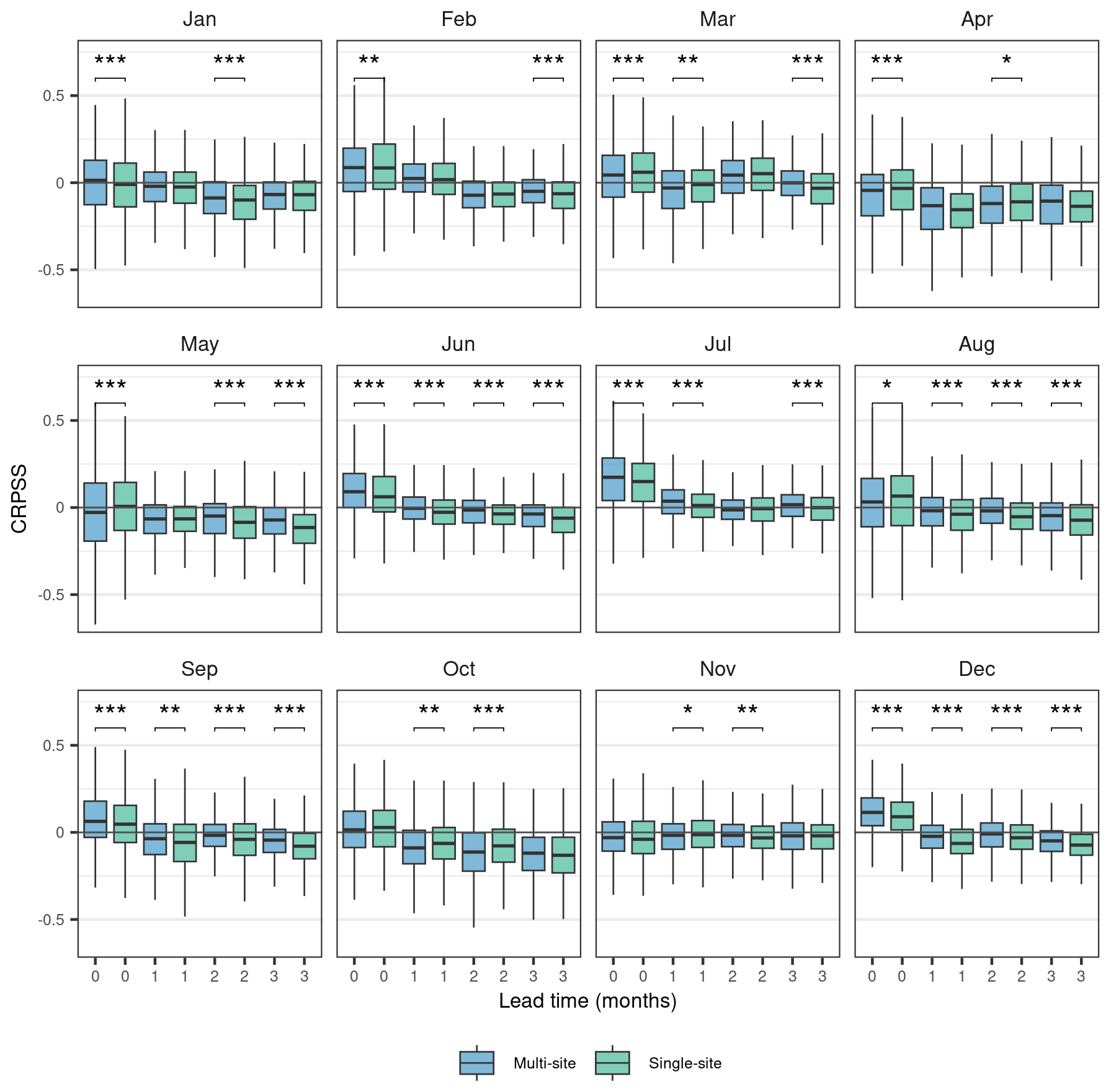
Figure 3 Comparison of CRPSS values for all forecast locations between the single-site model (green) and the multi-site model with catchment attributes (blue) by month. The skill score uses a reference forecast of climatology. We used a one-sided Wilcoxon signed-rank test to assess whether differences in skill scores between the models were significant (${}^{***}=p\mathit{<}\mathrm{0.001}$, ${}^{**}=p\mathit{<}\mathrm{0.01}$, ${}^{*}=p\mathit{<}\mathrm{0.05}$).

We used the Gini index to assess the importance of each predictor variable to the multi-site model with catchment attributes at each lead time (Fig. 2c). Monthly precipitation forecasts have high importance across lead times, while mean temperature forecasts have moderate importance. We also included antecedent conditions from observed streamflow and forecast precipitation. Antecedent streamflow is the most important variable at 1-month lead time but decreases with importance at later lead times. This is because we are limited to providing antecedent conditions prior to forecast initialisation, which has decreasing relevance as the lead time increases, reflecting our general understanding of the influence of initial versus boundary conditions in S2S hydrologic forecasting (e.g. Wood et al., 2016).

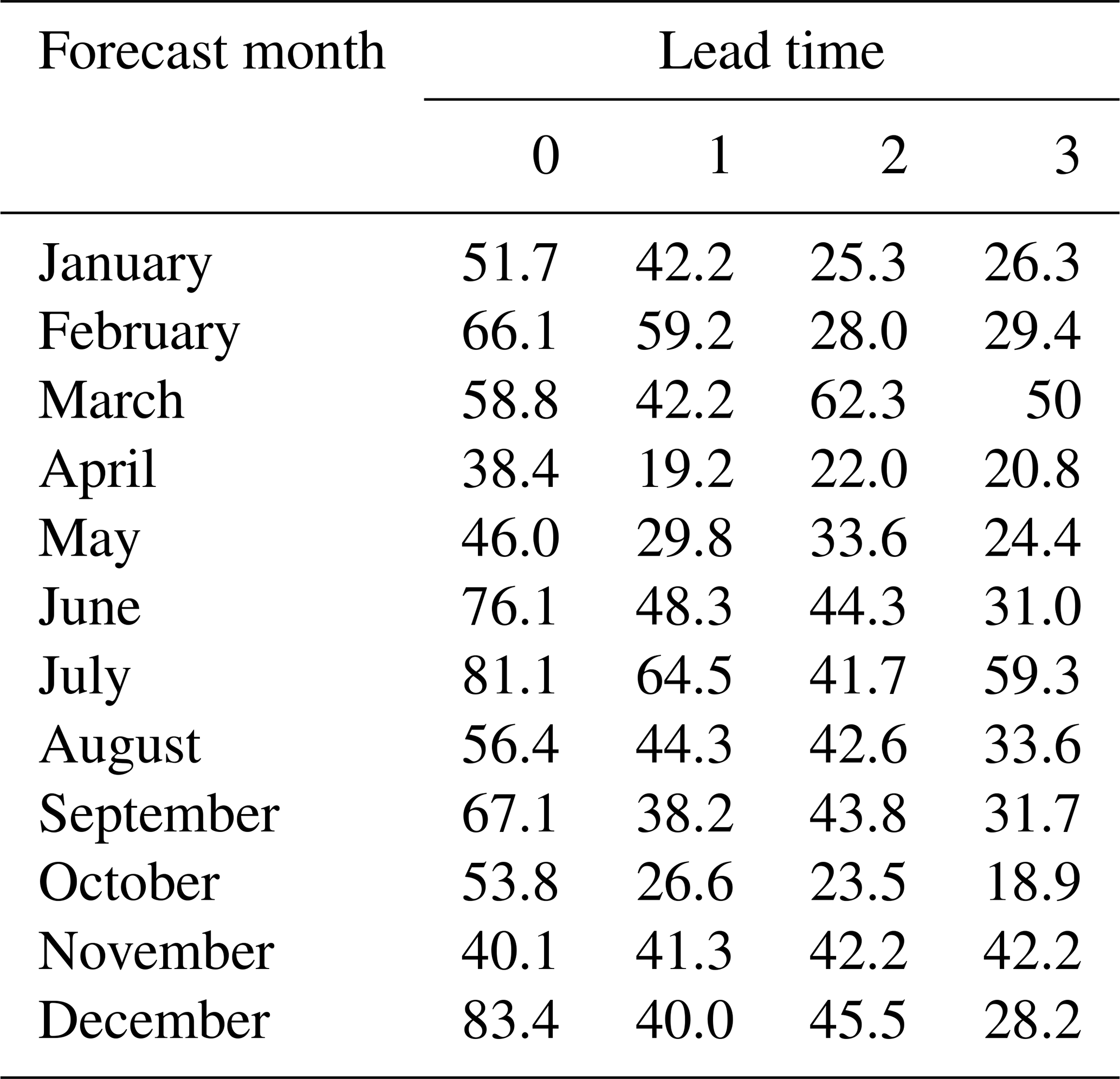
We assessed skill by computing the monthly CRPSS using a climatological prediction as a reference. We find that there is significant variability in skill during the different months of the year (Fig. 5a), especially at shorter lead times. For lead time 0, we observed the highest skill in extended winter (DJFM) and late summer (JJAS), with lower skill during spring and autumn. This is a positive result because, in the UK, high river flows are usually seen during the winter months. In December and July, more than 80 % of stations have positive skill in lead time 0 (Table 2). In most months, the skill decreases sharply over time, whereas, for other months (e.g. March), the skill remains relatively consistent as lead time increases. The variation in skill likely reflects both the varying importance of antecedent conditions during the year and the varying skill of the climate forecasts.

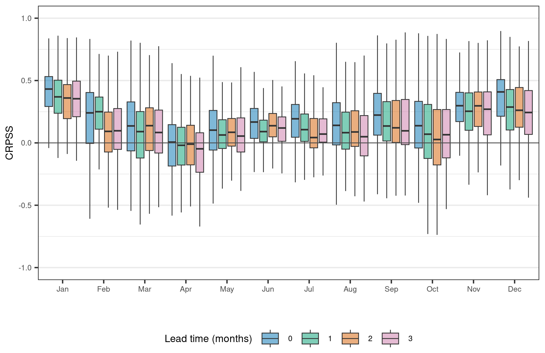
Figure 4 Continuous rank probability skill score of the multi-site model with catchment attributes using bias-corrected EFAS seasonal hindcasts as a benchmark.

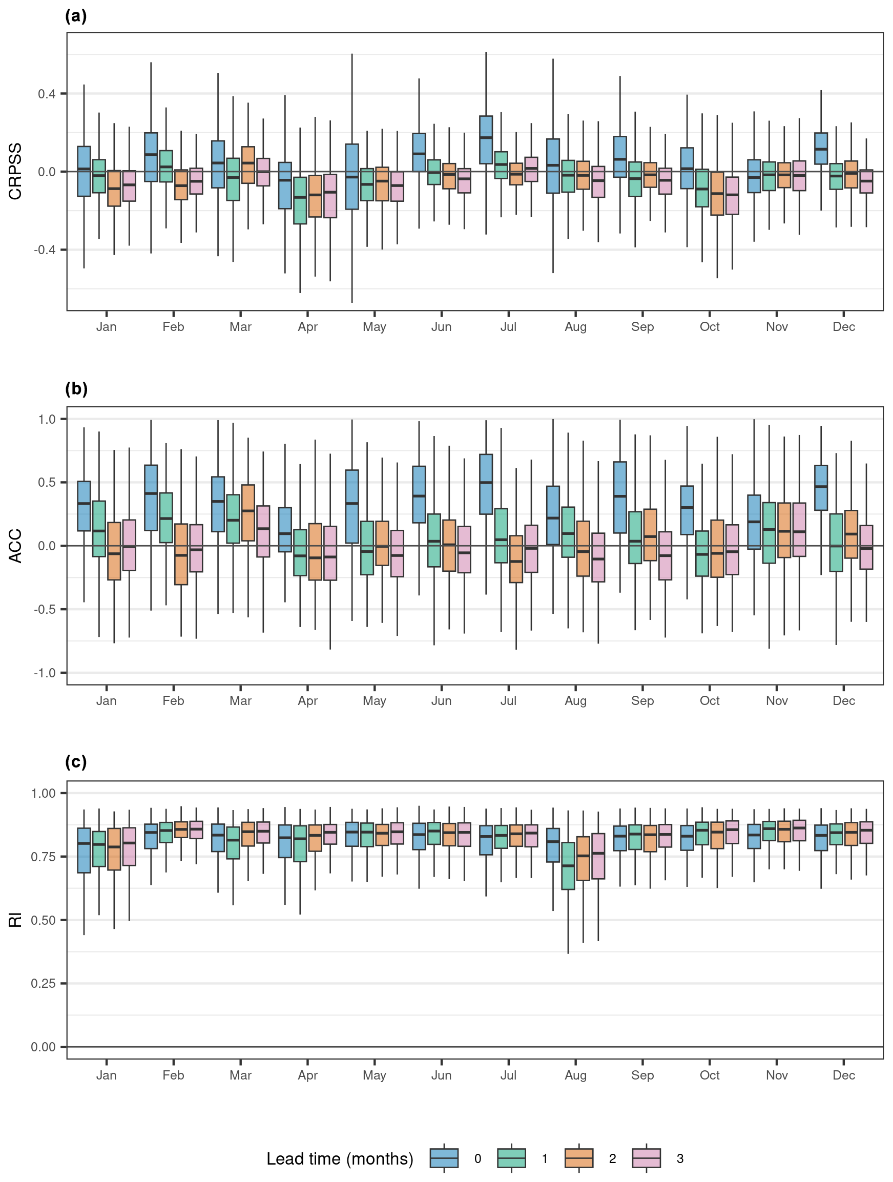
Figure 5 Performance assessment of the multi-site model with catchment attributes for each forecast month and lead time, using an ensemble climatological forecast as the reference. (a) Continuous ranked probability skill score (CRPSS). We use climatological forecast as the reference forecast, which is computed separately for each test year in the simulation. (b) Anomaly correlation coefficient (ACC). (c) Reliability index (RI). The four lead times are shown with different colours.

As with the CRPSS, the ACC varies by forecast month and lead time (Fig. 5b), with the monthly variability in the ACC following a similar pattern to that of the CRPSS. At lead time 0, the ACC is positive in >75 % of stations across all months. During lead time 1, the ACC is positive in >50 % of stations in all months except April, May, and October. Compared to the CRPSS and the ACC, the RI is more consistent across months and lead times (Fig. 5c). Overall, our ensemble hindcasts have high reliability, with the mean RI across all stations exceeding 0.8 in all months except August.

We also compared our results to monthly Q_max drawn from daily EFAS seasonal predictions for a subset of the stations included in this study (n=188) that overlapped with the EFAS reference dataset. We bias-corrected the EFAS outputs using a quantile mapping approach employing an empirical cumulative distribution function so that they could be directly compared with observations. As EFAS produces daily streamflow estimates, we took the maximum daily streamflow prediction from each month and used this value as the reference forecast to estimate the CRPSS. Our results are skilful compared to EFAS (Fig. 4), and this high relative skill, coupled with the general lack of positive skill of the QRF forecast for lead times of 1–3 months compared to a climatological reference, indicates that the EFAS predictions were poorer than expected as a benchmark for this monthly extreme target variable. We note that our model is specifically trained to predict Q_max, while EFAS seasonal forecasts are developed for more general purposes, such as supporting tercile probability forecasts for monthly or seasonal mean conditions, a common S2S hydrological product (e.g. Arnal et al., 2018).

Table 2 Percentage of stations (n=579) that are skilful (CRPSS > 0) compared to climatological reference forecast at each lead time and forecast month for the multi-site model with catchment attributes.

We examined the spatial variability in model skill by averaging the monthly skill scores for the multi-site model (with catchment attributes) within each season (Fig. 6). At lead time 0 we observe skill across much of the UK, while, at later lead times, skilful catchments tend to cluster in southern England. This could be related to the presence of relatively slower responding catchments with greater subsurface storage in the southeastern UK. However, we found relatively weak correlation between the ACC and the baseflow index (R=0.33, 0.31, 0.27, 0.25 for the four lead times). We observe a tendency for the QRF models to underestimate the observed Q_max, especially the more extreme values (Fig. 7). The underestimation is more pronounced as lead time increases, likely due to greater noise in the seasonal climate forecasts at longer lead times.

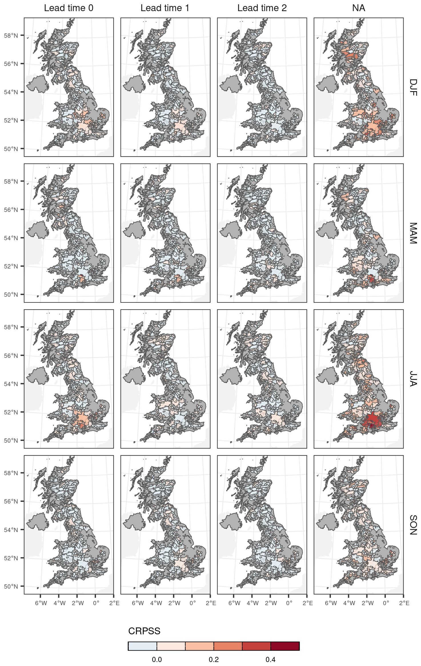
Figure 6 Average seasonal skill compared to climatological reference forecast in every catchment by lead time. We calculate the CRPSS per month and catchment and then compute the seasonal average (DJF, MAM, JJA, SON).

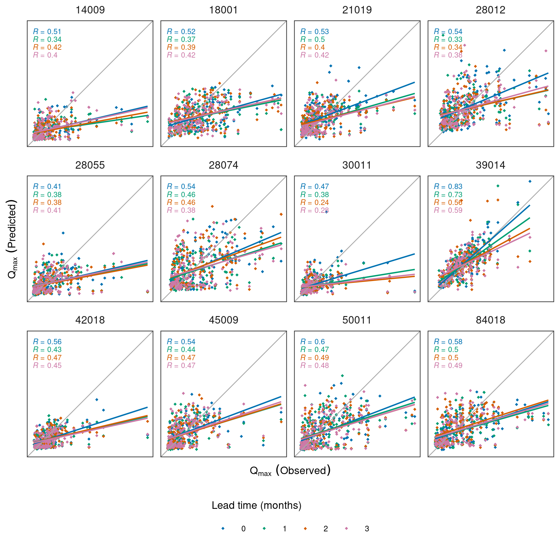
Figure 7 Comparison of observed and predicted Q_max across all months for 12 randomly selected catchments by lead time.

4 Discussion

We developed a hybrid forecasting approach for UK flood risk prediction at subseasonal to seasonal timescales using a large multimodel ensemble of climate predictions. Addressing our first research question, we found that S2S flood predictions are generally skilful (CRPSS > 0) up to 1 month following initialisation but that skill declines thereafter. However, 90 stations out of 579 retained positive skill in at least 3 months of the year for all four lead times. Across all initialisation times, 60 % of stations show positive skill compared to the climatological benchmark in the first month after initialisation. This proportion drops to 41 % in the second month, 38 % in the third month, and 33 % in the fourth month. The level of skill varies within the year, with some months generally more skilful than others. The seasonal variation in skill is likely due to a combination of varying climate predictability and the varying importance of antecedent conditions to flood magnitude and frequency during the year. The underlying seasonal forecasts of precipitation and temperature are also most skilful at shorter lead times, although they retain some information at longer lead times.

Our work provides guidance on how to build hybrid streamflow prediction systems that combine ML with dynamical model forecasts. With respect to our second research question, we found that a large-sample ML model trained on data from all catchments at once tends to outperform single-site model forecasts across all lead times. This results aligns with previous research on ML-based hydrological modelling, which revealed the benefit of a larger training dataset in large-sample models relative to single-site approaches (e.g. Kratzert et al., 2019). However, our work specifically considers forecasting months ahead, whereas previous work only studied out-of-sample simulation or short-term prediction using observed meteorological or weather forecast inputs. The large-sample approach enables ML models to combine information across time and space into a single model that is trained to discriminate a range of hydrological behaviours. The inclusion of static catchment attributes enables such models to learn the different rainfall–runoff behaviours across many catchments. This is especially important when using ML to predict extremes when training data are limited in time, as it means multi-site models remain realistic over a larger range of conditions than single-site models.

Hybrid prediction systems require training and testing partitions to evaluate model performance, and different approaches exist to do this. Here we implemented a forward-chain cross-validation approach such that the model is never trained on data more recent than the test partition. This reproduces an operational setup as far as possible, where the model is never exposed to information from the future. However, one limitation of this approach for hindcast studies is that the relatively short hindcast period of the C3S multimodel ensemble (i.e. 1994–2016) means the smallest training partition may contain as little as 10 years of monthly data. Nevertheless, during model development, we found that increasing the length of the training period (by focusing on the predictions from the SEAS5 system, which has an extended hindcast period of 1981–2016) did not significantly enhance the performance of the QRF models (results not shown). Moreover, using a multi-site approach reduces the impact of the relatively short reforecast period by pooling data from many catchments to create a much larger training dataset than is used by single-site models (i.e. swapping space for time).

Our hybrid seasonal flood forecasts based on eight models from the C3S multimodel ensemble exhibit relatively low skill, as is also the case with traditional (i.e. process-based hydrological model) flood forecasting systems driven by C3S (e.g. Arnal et al., 2018). These findings suggest that the primary constraint on enhanced skill lies in the seasonal climate forecasts. Increasing the skill of climate forecasts is therefore a priority to achieve more useful seasonal streamflow forecasts. One area for further research is to develop ways of identifying ensemble members that are likely to be more skilful over a given time period. Selecting members based on their ability to reproduce large-scale climate patterns, such as the North Atlantic Oscillation (NAO), is one potential option that has proved successful in other applications (e.g. Dobrynin et al., 2022; Moulds et al., 2023). Observed climate states, teleconnections, and indices (e.g. describing El Niño, the Southern Oscillation, and other climate modes) may be similarly exploited in regions where they exert an influence on weather patterns. These patterns have been deployed in empirical hydrologic forecast systems for many years, while the operational outputs from climate forecast models remain a relatively less explored source of predictability in hybrid approaches.

5 Conclusion

Operational services for seasonal streamflow forecasts have existed for over 1 century, offering highly skilled predictions in many parts of the world, and particularly when and where predictors with long persistence (such as snowpack or groundwater) and strong climate seasonality are present. Despite their successes, there is growing demand from stakeholders for improved seasonal flow prediction skill at times and in places where it has been more difficult to achieve, usually due to data limitations or hydroclimate considerations.

This study illustrates that a hybrid multi-site forecasting approach trained over a large-sample collection of watersheds may offer benefits for monthly to seasonal predictions of streamflow. Our approach affords users significant flexibility to define target variables of interest (e.g. Q_max). We use static catchment attributes as predictor variables to allow the QRF model to learn the different relationships between hydroclimate input data and monthly maximum daily streamflow, demonstrating an ability to produce skilful seasonal forecasts of monthly flood risk up to 4 months ahead in a moderate fraction of the catchments studied. The use of a multi-site ML model that is trained on data from multiple catchments at once may help to alleviate the long-standing problem of small sample sizes when training seasonal predictions on individual sites alone while also enabling prediction in ungauged basins. However, although the performance benefit of the multi-site model over single-site models is statistically significant, the improvement is modest, suggesting that the primary constraint on enhancing skill remains the quality of seasonal climate forecasts themselves.