Enhanced evaluation of hourly and daily extreme precipitation in Norway from convection-permitting models at regional and local scales

Convection-permitting regional climate models (CPRCMs) have demonstrated enhanced capability in capturing extreme precipitation compared to regional climate models (RCMs) with convection parameterization schemes. Despite this, a comprehensive understanding of their added values in terms of daily or hourly extremes, especially at the local scale, remains limited. In this study, we conduct a thorough comparison of daily and hourly extreme precipitation from the HARMONIE Climate (HCLIM) model at 3 km resolution (HCLIM3) and 12 km resolution (HCLIM12) across Norway's diverse landscape, divided into five regions, using both gridded and in situ observations. Our main focus is on investigating the added value of CPRCMs (i.e., HCLIM3) compared to RCMs (i.e., HCLIM12) for extreme precipitation from regional to local scales and on quantifying to what extent CPRCMs can reproduce the orographic effect on extreme precipitation at both daily and hourly scales. We find that HCLIM3 matches observations better than HCLIM12 for daily and hourly extreme precipitation across most grid points in Norway, while HCLIM12 underestimates the extremes, especially for hourly extremes. At the regional scale, HCLIM3 captures the maximum 1 d precipitation (RX1 d) and the maximum 1 h precipitation (Rx1 h) more accurately across most regions and seasons, with some exceptions. Specifically, for daily extremes, it shows larger summer biases in the east, south and west, as well as return levels biases in the east; for hourly extremes, larger biases are observed in the summer and in the west compared to HCLIM12. Besides this, for the local scale, HCLIM3 also outperforms HCLIM12 in most regions and seasons, except for a slightly larger summer bias in terms of daily extremes in the south and west. Overall, HCLIM3 consistently demonstrates added value in simulating daily extremes in the middle and northern regions at both regional and local scales, as well as in simulating hourly extremes at all 10 stations, compared with HCLIM12. Both HCLIM3 and HCLIM12 capture the seasonality of daily extremes well, while HCLIM3 performs better for the hourly extremes, accurately representing their frequency and intensity. Additionally, both models capture the reverse orographic effect of Rx1 h at the regional scale, with no added value seen in HCLIM3, while, at the local scale, HCLIM3 shows added value compared to HCLIM12 in representing the reverse orographic effect of Rx1 d in all seasons except summer. This study highlights the importance of more realistic CPRCMs in providing reliable insights into the characteristics of precipitation extremes across Norway's five regions. Such information is crucial for effective adaptation management to mitigate severe hydro-meteorological hazards, especially for the local extremes.

1 Introduction

In recent years, the world has witnessed a surge in both the frequency and the intensity of floods, primarily attributed to the increasing occurrence of intensive rainfall events (Tabari, 2020). These changes underscore the pressing need to develop a predictive understanding of precipitation extremes for the upcoming decades given the ongoing global warming. The intensification of precipitation extremes under the influence of global warming has the potential to trigger severe natural hazards and to result in significant socioeconomic impacts (Thackeray et al., 2022); this has gained substantial attention in recent research endeavors. However, most previous research in this field relied on coarse-resolution global climate models (GCMs) with grid sizes exceeding 100 km, which struggle to accurately simulate extreme-precipitation events and their frequency due to the limitations of their coarser resolution (Piani et al., 2010; Wang et al., 2017). Notably, these GCMs tend to produce the largest errors in predicting extreme precipitation, particularly in cases involving heavier convective activity, as observed in the study by Gervais et al. (2014a). Despite various bias correction techniques being applied to mitigate these discrepancies in the GCMs and despite their employment as forcing data for regional climate models (RCMs) with grid sizes larger than 10 km, it remains a persistent challenge to eliminate the transfer of biases from GCMs to RCMs, as noted by studies such as Pontoppidan et al. (2018) and Kim et al. (2020). The large resolution gap between GCMs or RCMs and localized precipitation extremes further constrains the robust simulations of extreme precipitation, as highlighted by Li et al. (2020a). In addition, the reliance on parameterization schemes to represent convection in these coarse-resolution models introduces a significant source of uncertainty in modeling errors (Prein et al., 2015; Kendon et al., 2019). More frequent and intense precipitation events under global warming stimulate interest in the use of higher-resolution and physics-based models to improve the estimation of short-duration extremes.

Convection-permitting regional climate models (CPRCMs) with grid sizes of less than 4 km offer a promising alternative as they explicitly represent convection, eliminating the need for parameterizations of deep atmospheric convection. The potential for resolving deep convection and local extremes from CPRCMs leads to the realistic representation of daily and sub-daily precipitation features, including diurnal cycle, intensity and frequency of heavy-precipitation events, seasonality, spatio-temporal pattern, and wet spells and dry spells. For instance, CPRCMs have been proven to reduce the bias and to enhance the representation of precipitation intensity and frequency in the Tibetan Plateau, the highest highland in the world, as shown in Li et al. (2021). In addition to their capability in capturing precipitation, Liu et al. (2017) also demonstrated the confidence of CPRCMs in estimating snowfall and snowpack in the central US. Furthermore, the importance of CPRCMs in representing dry spells and dry and wet extremes induced by local convective activity across Africa has also been found by Kendon et al. (2019); Chapman et al. (2023) further confirmed the benefit of CPRCMs with regard to capturing rare rainfall extremes and local features. In the UK, Kendon et al. (2023) and Kent et al. (2022) found the benefit of CPRCMs compared to RCMs with convection parameterization schemes. Additionally, the superior performance in capturing hourly and daily extreme precipitation, including return level, frequency and intensity, when using CPRCMs over Alpine areas has also been highlighted by Adinolfi et al. (2021), Dallan et al. (2023), and Giordani et al. (2023).

Northern Europe has been reported to experience a strong increase in precipitation, as indicated by Dyrrdal et al. (2023). Thus, a novel CPRCM has been developed within the Nordic Convection Permitting Climate Projections project (NorCP) based on the HARMONIE-Climate model (HCLIM) cycle 38 (HCLIM38; Belušić et al., 2020) and applied at a resolution of 3 km (HCLIM3). To investigate the added value of the convection-permitting resolution, HCLIM38 has also been run at a (non-convection-permitting) resolution of 12 km (HCLIM12). For convenience, HCLIM3 and HCLIM12 are used in the following to represent the HCLIM38 simulations at the two resolutions, i.e., the CPRCM and ordinary RCM, respectively. The term HCLIMs indicates the two of them, HCLIM3 and HCLIM12.

Through comparisons of seasonal precipitation; daily mean precipitation; higher-intensity daily precipitation; and diurnal cycle or hourly precipitation, including the frequency and intensity, from HCLIM3 and HCLIM12 over Fenno-Scandinavia, Lind et al. (2020) emphasized the added value of CPRCMs in reproducing extreme precipitation, primarily over complex terrain, compared to a coarser-scale model. Médus et al. (2022) also noted that the summer diurnal cycle of the frequency and intensity of hourly precipitation was correctly captured in HCLIM3 compared to in HCLIM12 in the Nordic region, with HCLIM12 underestimating the diurnal cycle. However, the evaluation and conclusions from Lind et al. (2020) and Médus et al. (2022) mainly focused on the large regional and country scales of Fenno-Scandinavia, overlooking the added values of CPRCMs at the local scale. Furthermore, Thomassen et al. (2023) observed that HCLIM3 tends to exhibit underestimations in monthly precipitation and a later evening peak compared to sub-kilometer models. They found that the advantages of sub-kilometer models were not outstanding. These evaluations were based on gridded datasets, which introduce uncertainty at the local scale, especially over complex orography (Lussana et al., 2019). As Chapman et al. (2023) demonstrated, underscoring the importance of assessing rare extreme-rainfall events in eastern African using convection-permitting models and parameterization convection models at both grid and station scales, the extremes from grids representing rainfall averaged over a larger area are damped. They found that the station-derived shape parameters and return levels are aligned with observations and suggested the significance of site-specific analysis and evaluations. The error induced by station density in gridded datasets has also been indicated by Gervais et al. (2014b), who made suggestions regarding the source of large errors in gridded datasets when station density is low. Consequently, a comprehensive evaluation and analysis of the added value from CPRCMs compared with RCMs, incorporating both the regional and local scales, is crucial for extreme precipitation.

We acknowledge that Norway, a Nordic country, is representative of diverse climate features due to its extended latitude, rugged coastline, plateaus and complex orography. The dominance of precipitation between the coastal and inland regions over Norway is distinctly different, and most of the studies focusing on the hydrology and meteorology over Norway were based on the divided regions (Vormoor et al., 2016; Poujol et al., 2021; Konstali and Sorteberg, 2022). By dividing regions according to their characteristics, a more thorough comprehension of the added value of CPRCMs in capturing extreme precipitation can be reached. Therefore, reliable evaluations of analyzing the added value of CPRCMs in capturing extreme precipitation should be scaled to the regional or local scale.

In complex mountain areas, extreme precipitation is triggered by the interaction of large-scale atmospheric activity and local orography properties, which may cause severe hydro-meteorological hazards, such as flash flooding. However, understanding the orographic impact of precipitation on complex orography is challenging due to sparse observations (Rossi et al., 2020). The poor representation of RCMs in capturing local precipitation has been indicated in Knist et al. (2020). Importantly, CPRCMs show advantages in reproducing precipitation over more highly complex orography in Alpine areas, as shown in Lind et al. (2016) and Reder at al. (2020). Furthermore, the better representation of sub-daily and daily heavy precipitation by CPRCMs over Alpine areas has also been found by Ban et al. (2020) and Dallan et al. (2023). Marra et al. (2021) and Dallan et al. (2023) also confirmed the efficiency of CPRCMs in reproducing the reverse orography effect on hourly extreme precipitation. The relationship between extreme precipitation and elevation may vary depending on latitude and climate zones (Amponsah et al., 2022). Rossi et al. (2020) and Mahoney et al. (2015) found a weak dependence of sub-daily precipitation on elevation in Colorado, USA. Opposing the orographic enhancement of daily precipitation, Dallan et al. (2023) indicated that there is no evident relationship between daily precipitation and elevation. It is worth noting that the potential added value of CPRCMs in representing orographic effects compared to RCMs has not been explored. Moreover, the performance of CPRCMs varies with the season, which underscores the need to explore the orographic effects on seasonal extremes. Thus, we fill this knowledge gap by characterizing orographic impacts on hourly and daily extreme precipitation seasonally.

As highlighted by Konstali and Sorteberg (2022), there can be significant uncertainties associated with the interpolation of gridded precipitation data. Besides this, the benefit of a spatial evaluation of precipitation based on in situ observations has also been reported in Thomassen et al. (2023). Therefore, here, the evaluation of extreme precipitation from HCLIM3 and HCLIM12 is based on both gridded precipitation and in situ observations. Our study aims to address the value of CPRCMs (HCLIM3) in capturing the characteristics of extreme precipitation in Norway, comparing it with a coarser-resolution model (HCLIM12), as well as both in situ and gridded precipitation observations. Here, our contribution to the existing literature, e.g., Médus et al. (2022), revolves around the added value of CPRCMs with regard to extreme-precipitation characteristics, encompassing a range of metrics.

The main objectives of this study are (1) to enhance the understanding of convection-permitting climate models and highlight the added value of CPRCMs by comparing their effectiveness in simulating extreme precipitation with that of regional climate models from regional to local scales and (2) to assess HCLIM3's capability in depicting orographic effects on seasonal extreme precipitation. This research explores whether the benefits provided by CPRCMs are consistent in different regions driven by varying physical processes relating to precipitation. Finally, our study delves into the analysis of the intensity and frequency of extreme-precipitation events, offering insights into local and regional variations.

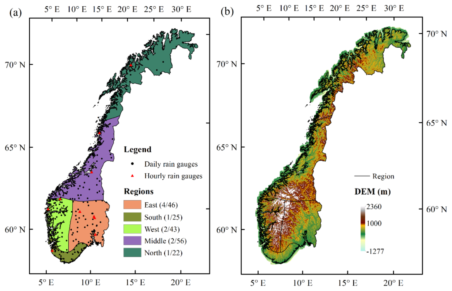
Figure 1 (a) The division of five regions in Norway. In the legend, the numbers shown in the brackets after each region represent the available size of hourly and daily stations in the region during 1999–2018. For example, “east (4/46)” means that there are available data from 4 hourly stations and 46 daily stations in the east during 1999–2018. (b) Spatial distribution of topography over Norway.

2 Study area and data

2.1 Study area

The different climate regimes between coastal and inland regions over Norway compel the analysis of hydro-meteorology based on divided regions. Based on similar seasonal cycle characteristics, Michel et al. (2021) and Konstali and Sorteberg (2022) divided the Norwegian continent into eight regions. Taking into account the spatial distribution of rain gauges and ensuring that each region has at least one hourly rain gauge, we combined the south and southwest into the south and the middle inland and north into the north. Therefore, in this study, mainland Norway is divided into five regions: east (E), south (S), west (W), middle (M) and north (N) (as shown in Fig. 1).

The study areas cover mainland Norway, which has unique climate characteristics within different regions. Precipitation in Norway primarily occurs along the coast in late autumn and winter, while inland areas receive more precipitation in summer. The eastern region, with stratiform precipitation originating from the south, is dominated by continental climate, with convective precipitation in summer. The western coast of Norway is strongly affected by the North Atlantic storm track, where precipitation from frontal systems and land-falling storms is enhanced due to the orographic uplift over Scandinavia (Poujol et al., 2021). Most extreme events occurring in the western region, with abrupt topography, are mainly related to atmospheric rivers (ARs), which are generally linked to extratropical cyclones during cooler seasons (Whan et al., 2020). Additionally, in the summer, ARs coincide with more frequent convective activities (Poujol et al., 2021). The southern region lies at the end of the climatological jet and is regularly affected by the ARs, especially during the zonal and Atlantic trough weather regimes (Michel et al., 2021), while convective activities play a crucial role in the southern regions in summer (Li et al., 2020b). For the middle and northern regions, 59 % of extremes are associated with ARs, and the precipitation rate decreases moving inland (Konstali and Sorteberg, 2022).

2.2 Data

We utilize the outputs of double-nested model simulations from the HCLIM38 model, which includes different configuration settings for each spatial resolution: HCLIM3 and HCLIM12. HCLIM12 covers most of Europe with 313 × 349 grid points using the ERA-Interim reanalysis (∼ 80 km) as the boundary condition, and HCLIM3 spans the Fenno-Scandinavian region with 637 × 853 grid points using the output of the HCLIM12 as the boundary condition for every 3 h. Importantly, the convection parameterization scheme was switched off in HCLIM3, allowing for an explicit representation of convection processes. The present-day simulations from HCLIM3 and HCLIM12 span the years 1997–2018. For more comprehensive information, refer to the work of Lind et al. (2020) and Médus et al. (2022).

This study primarily focuses on assessing the performance of HCLIM3 and HCLIM12 in simulating hourly and daily extreme-precipitation events in mainland Norway for the present-day period (1997–2018, with the first 2 years excluded). The model outputs from HCLIM3 and HCLIM12 are specifically extracted for mainland Norway. Before analysis, HCLIM3 data were remapped to the HCLIM12 grid (12 km) using a bilinear interpolation method.

Precipitation from the SeNorge_2018 (SeNorge) gridded dataset, covering Norway with 1 d temporal resolution and 1 km spatial resolution since 1957 (Lussana et al., 2019), is used as the observation dataset to evaluate the performance of HCLIM3 and HCLIM12 during 1999–2018. Precipitation from the SeNorge2 gridded dataset, with 1 h temporal resolution and 1 km spatial resolution, is also applied to evaluate the hourly result during 2010–2018 (Lussana et al., 2018). In addition, in situ precipitation observations, including both 1 h and 1 d resolutions, are downloaded from the Norwegian Meteorological Institute Frost API (https://met.no, last access: 24 April 2025).

3 Methods

3.1 Evaluation of precipitation

To evaluate the characteristics of precipitation extremes between HCLIM3 and HCLIM12, we compared the historical simulations with the daily SeNorge gridded dataset, the hourly SeNorge2 gridded dataset and in situ observations. We only keep the stations that have less than 10 % of the data missing during 1999–2018 and consider station distribution uniformity, giving a total of 192 daily stations and 10 hourly stations, over Norway (Fig. 1, Tables S1 and S2 in the Supplement). In this study, the evaluation based on in situ observations and gridded datasets (SeNorge and SeNorge2) was defined at the local scale and regional scale, respectively.

Remapping finer-resolution data to a coarser resolution reduces the influence of such artifacts by averaging out the variability. This approach is consistent with the methodology used by Lind et al. (2020) and Médus et al. (2022), who also remapped all data to a coarser grid when comparing the performance of HCLIM3 and HCLIM12. Lind et al. (2020) observed that the differences between HCLIM3 data remapped to the coarser native grid of HCLIM3 and the HCLIM12 grids were minimal. Importantly, they found that the improvements in HCLIM3 persisted even after spatial aggregation, indicating that the enhanced resolution of the model offered benefits that were preserved when viewed on a coarser grid. Therefore, HCLIM3, SeNorge and SeNorge2 were remapped to the HCLIM12 grid ∼ 12 km for the evaluation at the regional scale. For the SeNorge- and SeNorge2-based assessments, the extreme indices are first calculated at the grid point level, and then the regional averages are computed. For the evaluation based on in situ observations, HCLIM3 and HCLIM12 were interpolated to the 192 daily rain gauges and 10 hourly rain gauges to calculate the indices using a bilinear interpolation method.

For the evaluation of extreme precipitation, we examined the maximum 1 d precipitation (Rx1 d); maximum 1 h precipitation (Rx1 h); return-period-based precipitation amounts at 5-, 10-, 20- and 50-year return periods; and seasonality of frequency and/or intensity from the regional to local scale. The calculation of seasonal Rx1 d or Rx1 h was based on the maximum value within one season per year.

3.2 Extreme-precipitation indices

The generalized extreme value (GEV) distribution was used to estimate precipitation intensity for specific return periods (e.g., 5, 10, 20 and 50 years). The return levels were calculated by fitting the annual maximum discharge derived from observed and simulated daily data (both gridded and rain gauges) and hourly data (only 10 rain gauges) to the GEV distribution. Then the quantile Z_p of the GEV distribution with a return period of $\frac{\mathrm{1}}{p}$ can be obtained. The GEV distribution has been widely used to model extreme events in meteorology (Coles et al., 2003). The cumulative distribution function F(x) and probability density function f(x) of the GEV were used as follows to calculate the return level Z_p:

$$\begin{array}{}\text{(1)}& {\displaystyle }F\left(x\right)=\exp \left\{-{\left[\mathrm{1}-k\left({\displaystyle \frac{x-\mathit{\xi }}{\mathit{\alpha }}}\right)\right]}^{\mathrm{1}/k}\right\}k\ne \mathrm{0}\text{(2)}& {\displaystyle }\begin{array}{rl}f\left(x\right)& ={\displaystyle \frac{\mathrm{1}}{\mathit{\alpha }}}{\left[\mathrm{1}-k\left({\displaystyle \frac{x-\mathit{\xi }}{\mathit{\alpha }}}\right)\right]}^{\mathrm{1}/k-\mathrm{1}}\\ & \times \exp \left\{-{\left[\mathrm{1}-k\left({\displaystyle \frac{x-\mathit{\xi }}{\mathit{\alpha }}}\right)\right]}^{\mathrm{1}/k}\right\},\end{array}\text{(3)}& {\displaystyle }{Z}_{\mathrm{p}}=\mathit{\xi }-{\displaystyle \frac{\mathit{\alpha }}{k}}\left\{\mathrm{1}-{\left[-\log \left(\mathrm{1}-p\right)\right]}^{-k}\right\},\end{array}$$

where α, ξ and k indicate the scale, location and shape parameters, respectively. Kolmogorov–Smirnov, Anderson–Darling and chi-square tests were performed to determine if the GEV was accepted to fit the maxima series.

3.3 Quantification of the orographic effect

The orographic effect on Rx1 h and Rx1 d precipitation was explored by looking at the relationship of the annual and seasonal maxima with elevation from regional to local scales. A linear regression model (Di Piazza et al., 2011) was utilized to approximate the relations. The relationship of elevation with observations (Rx1 h (SeNorge2), Rx1 d (SeNorge) and daily in situ observation) and simulations (HCLIM3 and HCLIM12) was fitted to compute the linear regression slope. To eliminate the impact of the unit (Rx1 h and Rx1 d), the slope is converted to a relative slope with respect to the average value of extreme precipitation, expressed as percentage precipitation (%) per kilometer of elevation. This is done by dividing the mean extreme-precipitation value for the entire study region computed separately for daily and hourly extremes. The orographic effect at the local scale was only based on daily in situ observations due to the limited hourly in situ observations. At the local scale, the elevation for each rain gauge was extracted according to the digital elevation model. At the regional scale, the grid of the digital elevation model and HCLIM3 was resample to the same grid resolution as HCLIM12 (12 km) before calculation. Only the grids and stations above sea level (0 m) are included to quantify the orographic effect.

If the precipitation increases with elevation, there is an orographic effect on extreme precipitation; if the precipitation decreases with elevation, this results in a reverse orographic effect on extreme precipitation.

4 Results

4.1 Evaluation of daily extremes with SeNorge

4.1.1 Maximum 1 d precipitation (Rx1 d)

Figure 2 provides a comprehensive comparison of percentage biases of Rx1 d from HCLIM3 and HCLMI12 compared to SeNorge. From Fig. 2a, we can see that HCLIM12 has more grids with underestimated Rx1 d than HCLMI3 in Norway, which is confirmed clearly in Fig. 2b, showing a density plot of the percentage bias distribution from two models compared with SeNorge. Specifically, more grids from HCLIM3 than from HCLIM12 tend to overestimate Rx1 d within the 0 %–25 % range, while HCLIM12 leans towards larger underestimation within the −10 %–50 % range. The density curve in Fig. 2b reflects a higher peak at 0 for HCLIM3, indicating a more accurate representation of Rx1 d, with an average dry bias of 1.6 %. Conversely, HCLIM12 shows a 7 % dry bias for Rx1 d on average.

Figure 2c shows the absolute percentage bias of annual and seasonal Rx1 d from HCLIM3 and HCLIM12 compared to SeNorge for five regions in four seasons. Annually, HCLIM3 exhibits added value in capturing Rx1 h in the five regions compared to HCLIM12. HCLIM3 captures Rx1 d over four seasons and annually for five regions better than HCLIM12, while HCLIM12 shows larger bias in most regions, except in the east, south and west during summer. In summer, HCLIM3 only outperforms HCLIM12 with regard to Rx1 d in the middle and in the north. Overall, HCLIM3 shows notable added value in Rx1 d compared with HCLMI12 across regions and seasons, except in summer.

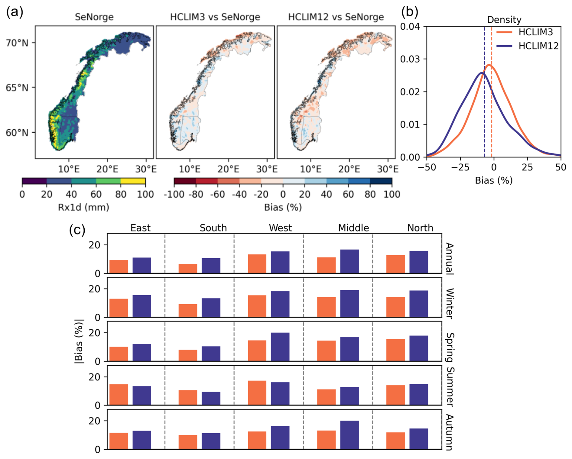
Figure 2 (a) The annual Rx1 d of SeNorge and the percentage bias of Rx1 d from HCLIM3 and HCLIM12 compared to SeNorge during 1999–2018; (b) density plot of the percentage bias distribution for annual Rx1 d from HCLIM3 and HCLIM12 compared to SeNorge for Rx1 d during 1999–2018 (the dashed lines represent the mean bias); (c) the absolute percentage bias of annual and seasonal Rx1 d from HCLIM3 and HCLIM12 compared to SeNorge for five regions. The bias is first calculated at the grid point level, and then regional averages are computed. For (a) and (b), the percentage bias is equal to model simulations minus observations, divided by observations. For (c), the absolute percentage bias is calculated as the absolute difference between simulations and observations, divided by observations.

Furthermore, as shown in Fig. 3, a comparison of the Rx1 h percentage biases of HCLIM3 and HCLIM12 with SeNorge2 for the period 2010–2018 demonstrates that HCLIM3 has a clearly added value in simulating the annual Rx1 h in Norway, with smaller wet biases on average, while HCLIM12 shows larger dry biases over the whole of mainland Norway. At the regional scale, HCLIM3 also shows added value in capturing annual and seasonal Rx1 h compared to HCLIM12 in five regions, excluding the western and middle regions. Specifically, in the western region, HCLIM3 exhibits larger absolute percentage biases than HCLIM12 in annual Rx1 h and seasonal Rx1 h, except in spring. In summer, only in the southern and northern regions is the Rx1 h bias of HCLIM3 smaller than that of HCLIM12.

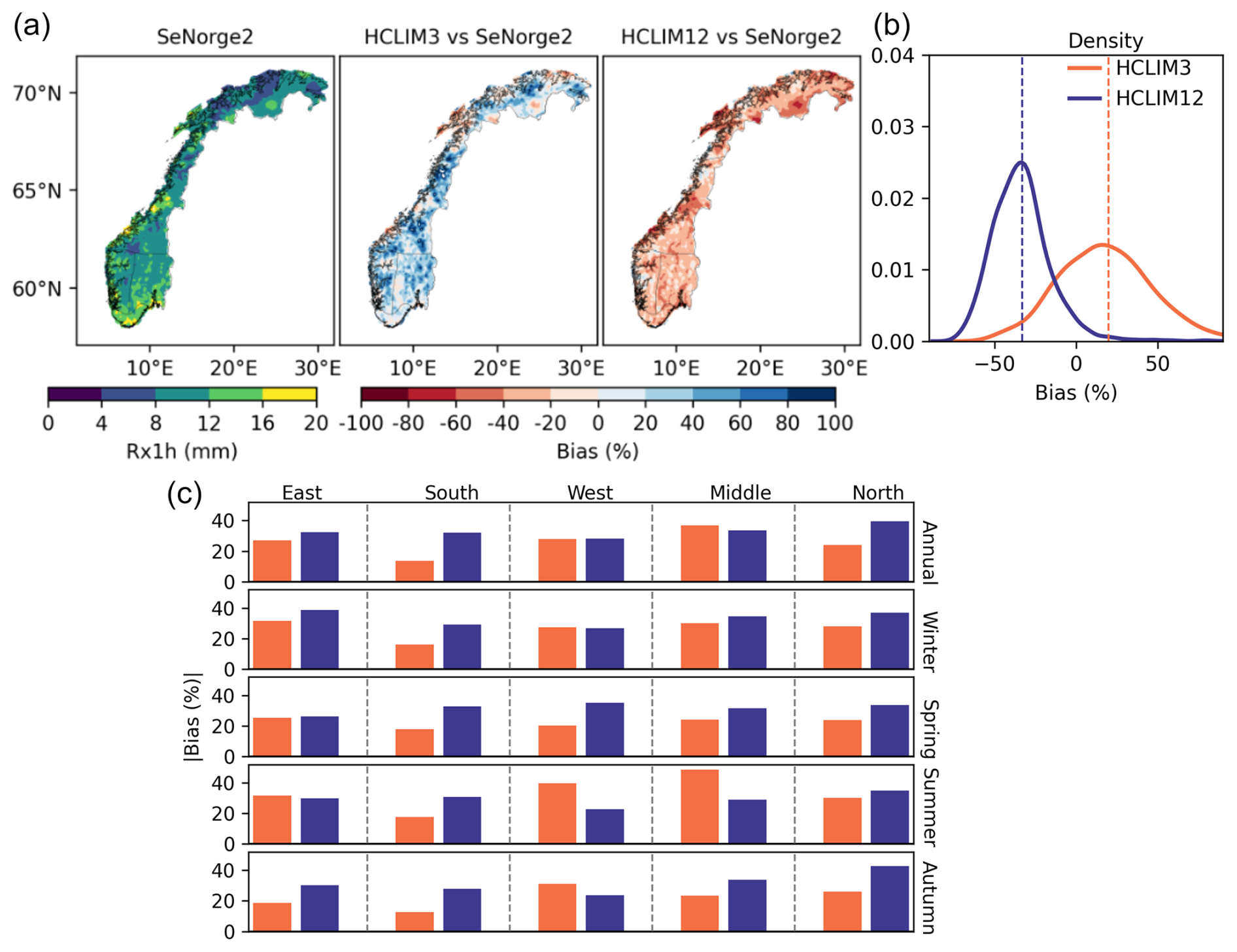
Figure 3 (a) The annual Rx1 h of SeNorge2 and the percentage bias of Rx1 h from HCLIM3 and HCLIM12 compared to SeNorge2 during 2010–2018; (b) density plot of percentage bias for annual Rx1 h distribution from HCLIM3 and HCLIM12 compared to SeNorge2 during 2010–2018 (the dashed lines represent the mean bias); (c) the absolute percentage bias of seasonal Rx1 h from HCLIM3 and HCLIM12 compared to SeNorge2 for five regions. For (a) and (b), the percentage bias is equal to model simulations minus observations, divided by observations. For (c), the absolute percentage bias is calculated as the absolute difference between simulations and observations, divided by observations.

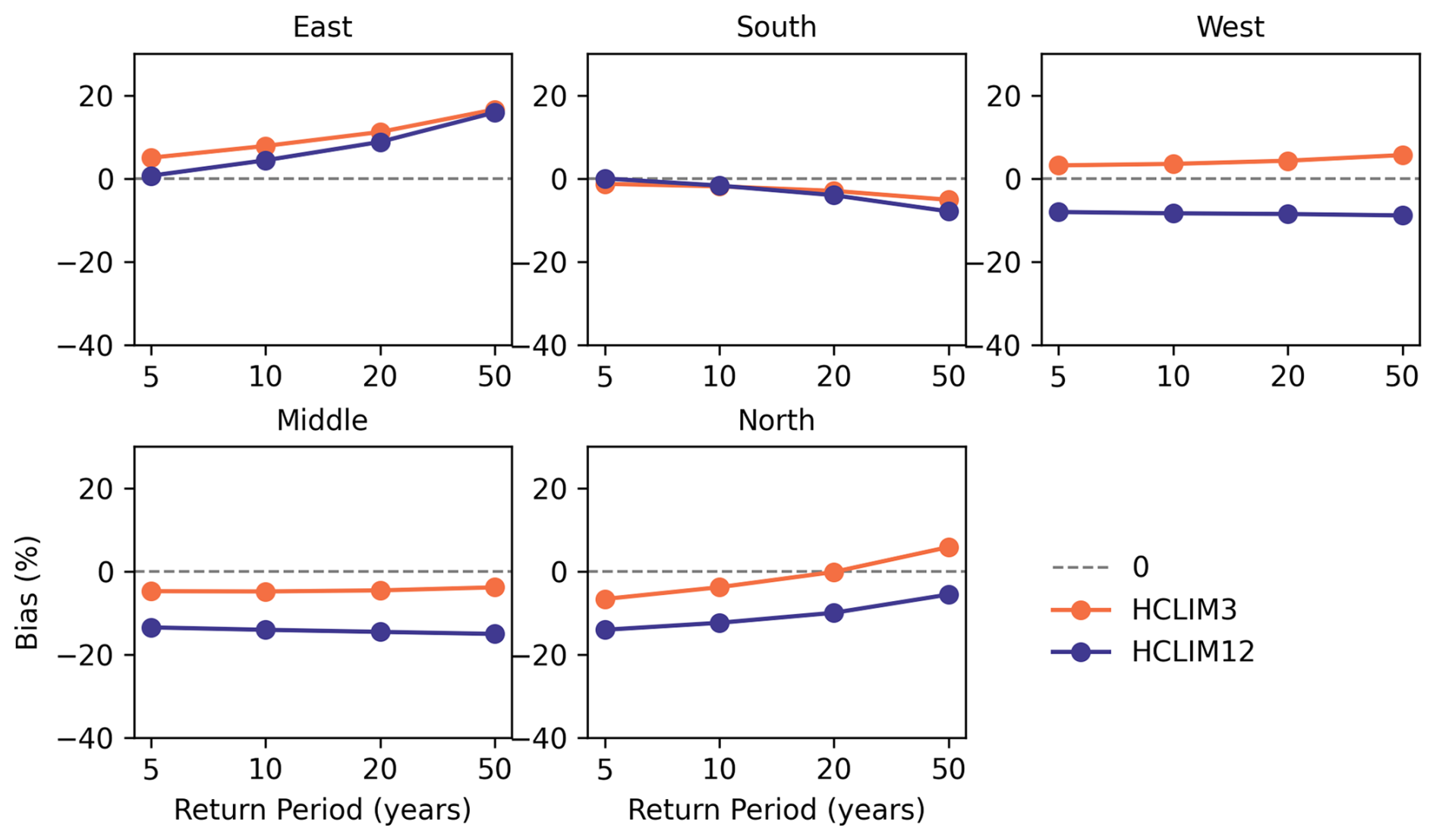
Figure 4 Percentage bias of extreme daily precipitation exceeding the 5-year to 50-year return periods over five regions between SeNorge and HCLIMs (i.e., HCLIM3 and HCLIM12). Return periods of 5, 10, 20 and 50 years are calculated on the basis of the GEV.

4.1.2 Return levels

Figure 4 shows the bias in estimated daily precipitation for 5-, 10-, 20- and 50-year return periods during 1999–2018 across five regions (compared to SeNorge). Great interregional variation is seen between HCLIM3 and HCLIM12. Relative to SeNorge, HCLIM3 tends to overestimate return levels in the eastern and western regions, while it underestimates them in the other regions. By comparison, except for the eastern region, where HCLIM12 shows overestimation, the extreme-precipitation estimates in most other regions are underestimated. The performance of HCLIM3 in capturing extremes varies across regions. HCLIM3 and HCLIM12 exhibit percentage biases of opposite sign in simulating return level precipitation in the western region, where HCLIM3 overestimates and HCLIM12 underestimates precipitation at different return periods. In the western, middle and northern regions, HCLIM3 outperforms HCLIM12 in all return periods, but the performance is less satisfactory in the eastern region.

Given the societal impacts of precipitation extremes, understanding how HCLIM3 and HCLIM12 represent these extremes is crucial. The physical processes driving precipitation in inland and coastal regions, as highlighted by Konstali and Sorteberg (2022), emphasize the need for a separate evaluation for each region with different characteristics. This approach ensures a more robust assessment, providing valuable information for regional authorities.

4.2 Evaluation of daily extreme with in situ data

4.2.1 Maximum 1 d precipitation (Rx1 d)

Similarly to the regional results in Fig. 2, Fig. 5 shows the percentage bias of annual and seasonal Rx1 d from HCLIM3 and HCLIM12 in comparison to in situ observations. Notably, a difference between HCLIM3 and HCLIM12 can be seen at the local scale compared to at the regional result: a greater number of sites from HCLIM3 approach zero bias, and more grids from HCLIM12 show a dry bias of about 10 %–40 %, as shown in Fig. 5b. On average, HCLIM12, with a 4.5 % dry bias, tends to underestimate annual Rx1 d, while HCLIM3 represents added value in capturing annual Rx1 d, with a 1 % wet bias, on average, at the local scale. Furthermore, HCLIM3 shows added value in simulating the annual Rx1 h at the local scale in all regions.

From a seasonal perspective, as shown in Fig. 5c, overall, HCLIM3 shows added value in capturing the seasonal Rx1 d in most regions and seasons, except for summer. Specifically, HCLIM3 performs better than HCLIM12, except for the western and southern regions, where HCLIM3 exhibits a larger bias in summer Rx1 d. In particular, the added value of HCLIM3 in simulating autumn Rx1 d in the east and west is not as obvious when compared to HCLIM12.

It is noteworthy that, at the local scale, HCLIM3 and HCLIM12 perform similarly compared to the regional results in most regions. There are some exceptions; e.g., HCLIM3 shows larger biases in summer Rx1 d in the south and west compared with HCLIM12 at both the regional and local scale. In contrast to the clearly larger bias in Rx1 h at the regional scale for both HCLIM3 and HCLIM12, a relatively smaller bias in Rx1 d is demonstrated at both the regional and local scale. At the regional scale, HCLIM3 exhibits added value in all seasons except summer, while, at the local scale, HCLIM3 and HCLIM12 show similar biases in autumn Rx1 d in the east and west, which means that the advantage of HCLIM3 over HCLIM12 at the local scale in autumn weakens in the west and east compared to at the regional scale.

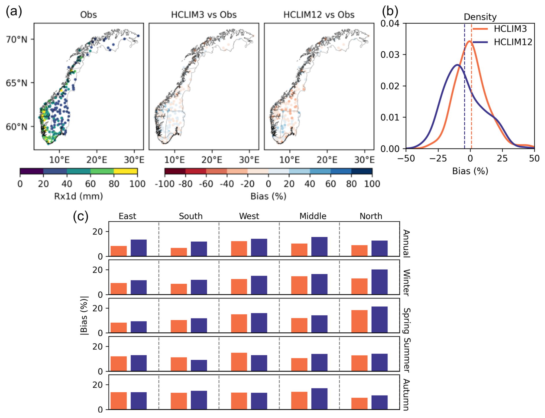
Figure 5 (a) The annual Rx1 d of in situ observations and the percentage bias of Rx1 d from HCLIM3 and HCLIM12 compared to in situ observations during 1999–2018 over 194 stations; (b) density distribution of percentage bias for annual Rx1 d between HCLIMs and observations from 194 stations during 1999–2018 (the dashed lines represent the mean bias); (c) the absolute percentage bias of seasonal Rx1 d between HCLIMs and observations across the five regions. For (a) and (b), the percentage bias is equal to model simulations minus observations, divided by observations. For (c), the absolute percentage bias is calculated as the absolute difference between simulations and observations, divided by observations.

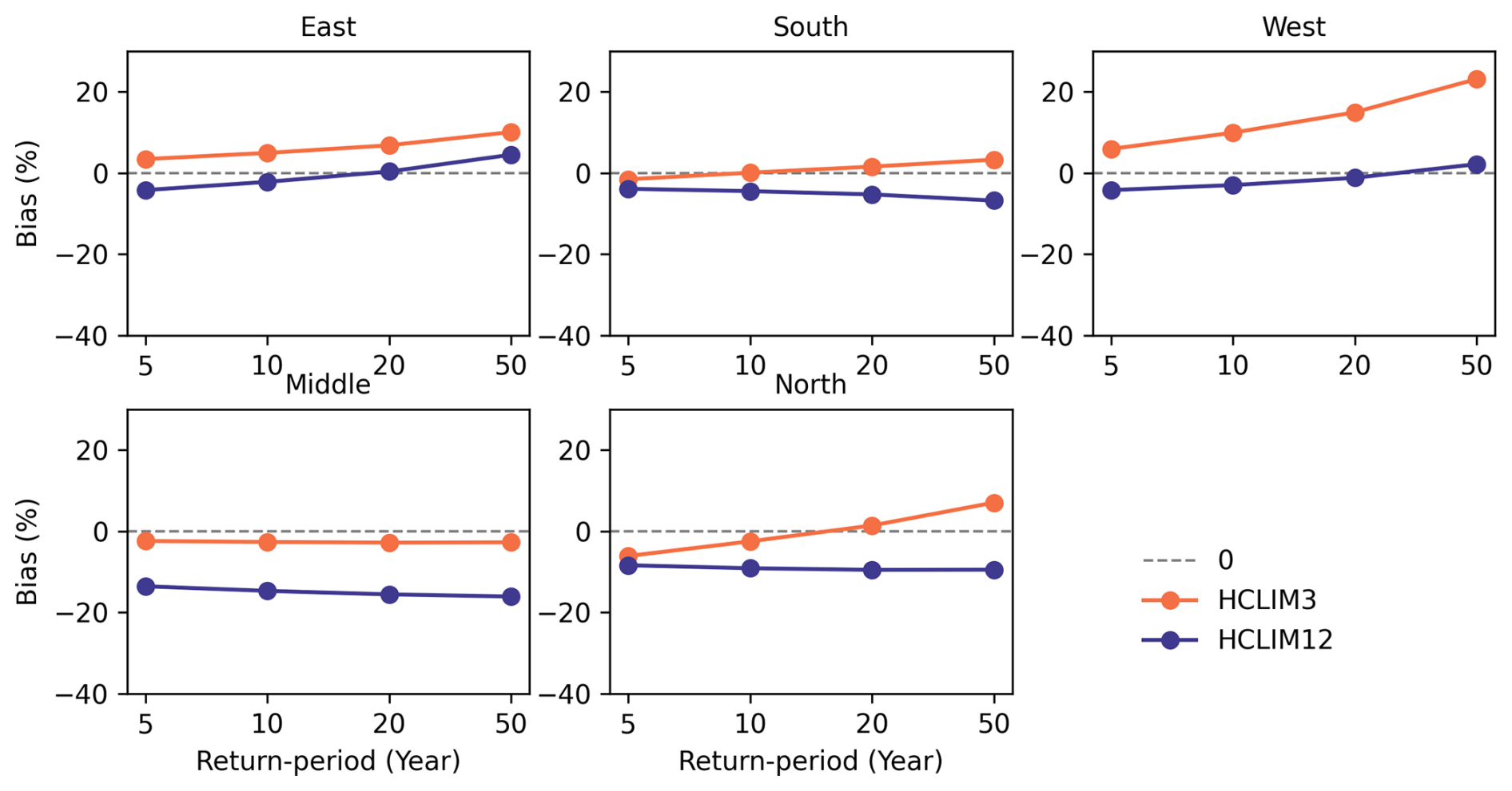
Figure 6 Percentage bias of extreme daily precipitation exceeding the 5-year to 50-year return periods over five regions between HCLIMs (i.e., HCLIM3 and HCLIM12) and in situ observations in the 192 daily rain gauges. Return periods of 5, 10, 20 and 50 years are calculated on the basis of the station-scale GEV.

4.2.2 Return levels

Figure 6 shows the percentage bias of the estimated daily return levels (e.g., 5-, 10-, 20- and 50-year return periods) from HCLIM3 and HCLIM12 compared to observations for the period 1999–2018. The figure illustrates the average bias of return levels for the stations in the corresponding regions. Compared with the in situ observations, HCLIM3 overestimates the return levels in the east and west for all return periods (5, 10, 20 and 50 years) and underestimates return levels in the south and north for the 20- and 5-year return periods, while HCLIM12 underestimates the return levels in all regions. Generally, HCLIM3 can more accurately represent the return levels in most regions compared to HCLIM12. The biases of HCLIM3 and HCLIM12 vary across regions and return periods. HCLIM3 has lower biases than HCLIM12 in most regions, except for the eastern and western regions. Both HCLIM3 and HCLIM12 perform well in the southern region. In addition, Fig. S1 shows the range of the return levels for all stations in the corresponding region, and HCLIM3 introduces larger variations in the western and southern regions compared with HCLIM12, as indicated by the wider whiskers.

4.3 Evaluation of hourly extremes with in situ data

4.3.1 Maximum 1 h precipitation (Rx1 h)

The time evolution of annual Rx1 h from HCLIM3 and HCLIM12 is compared to in situ observations during 1999–2018, as shown in Fig. 7. Compared to HCLIM12, HCLIM3 shows distinct superiority in capturing the time evolution of annual Rx1 h, even with underestimation and time shifting at some local locations. For example, HCLIM3 and HCLIM12 struggle to capture the annual Rx1 h above 25 mm h⁻¹ at Kvithamar (SN69150), Særheim (SN44300), Tromsø–Holt (SN90400), Tjøtta (SN76530) and Løken i Volbu (SN23500). However, HCLIM3 captures the annual Rx1 h in other local places well despite the time deviation of annual Rx1 h. Taking the site Østre Toten–Apelsvoll (SN11500) as an example to illustrate the time deviation, HCLIM3 simulates that the annual Rx1 h (37 mm) over the past 20 years occurred in 2001, 4 years earlier than the in situ observation (35 mm). Furthermore, to better assess the annual variability of Rx1 h, we extracted grids within a 12 km radius of each station and calculated the uncertainty range (Fig. S2), which reveals that the interpolated local Rx1 h precipitation from HCLIM12, particularly over grids with a larger area, tends to be damped, resulting in a narrower range than HCLIM3. Based on station statistics of annual mean Rx1 h in Norway, the boxplot (Fig. 7) shows that the annual mean Rx1 h of HCLIM3 is within the range of observed values. In contrast, HCLIM12 consistently underestimates Rx1 h, with all its values being below the observed minimum. Despite outperforming HCLIM12, it is noteworthy that HCLIM3 demonstrates limitations in reproducing the accurate occurrence time and magnitude of annual Rx1 h at the local level in Norway.

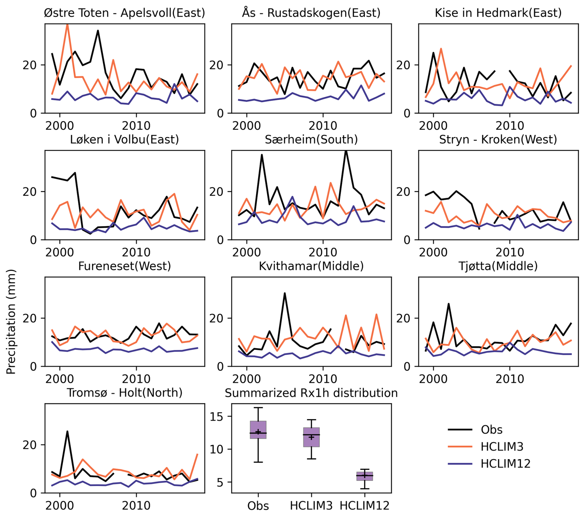
Figure 7 Time evolution of Rx1 h precipitation for each year from observations, HCLIM3 and HCLIM12 during 1999–2018 at 10 rain gauges (Table S1). The final boxplot summarizes the statistical distribution of Rx1 h from observations and both HCLIMs simulations.

4.3.2 Return levels

At the local and hourly scale, HCLIM3 has a better representation of hourly extreme events for the 5-, 10-, 20- and 50-year return periods compared to HCLIM12. Although both HCLIM3 and HCLIM12 tend to underestimate the annual Rx1 h for all return periods at almost stations (Fig. 8), the biases between the observations and the interpolated HCLIM3 for all 10 rain gauges are consistently lower than those of HCLIM12 for all return periods. The exceptions are Kvithamar (SN69150), Tromsø-Holt (SN90400) and Fureneset (SN56420), which present at all return periods, and Østre Toten–Apelsvoll (SN11500), which presents at a 50-year return period, where HCLIM3 shows a slight overestimation. Notably, the return levels of hourly extreme events at all 10 sites are accurately captured by HCLIM3, demonstrating its better ability to capture the extreme hourly precipitation for the 5-, 10-, 20- and 50-year return periods in localized areas compared to HCLIM12. This result underscores the added value of CPRCMs in representing hourly extreme precipitation at a very localized scale despite the overall underestimation of return levels by both HCLIM3 and HCLIM12.

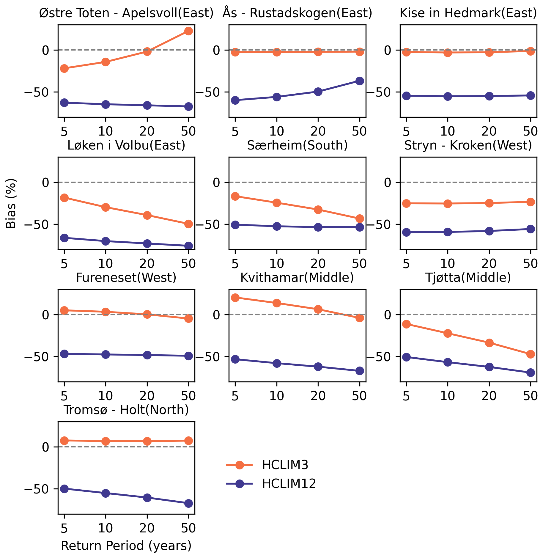
Figure 8 Percentage bias of extreme hourly precipitation exceeding the 5-year to 50-year return periods between HCLIMs (i.e., HCLIM3 and HCLIM12) and in situ observations in the 10 hourly rain gauges. Return periods of 5, 10, 20 and 50 years are calculated on the basis of the station-scale GEV.

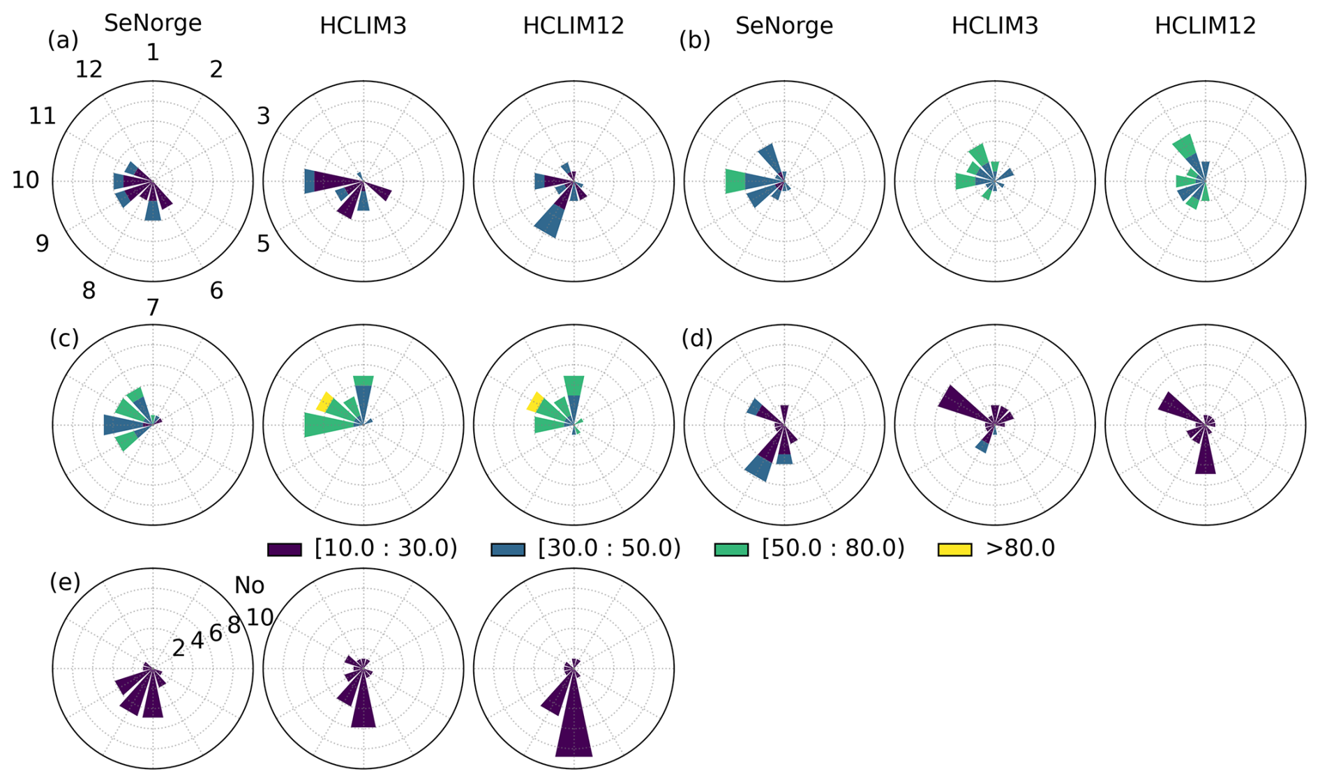
Figure 9 The seasonality of the frequency and magnitude of Rx1 d precipitation from SeNorge, HCLIM3 and HCLIM12 during 1999–2018 over different regions: (a) east, (b) south, (c) west, (d) middle and (e) north. Radial axis represents the frequency (“No.”). The color represents the magnitude of Rx1 d (mm). Winter: December, January, February; spring: March, April, May; summer: June, July, August; autumn: September, October, November.

4.4 Evaluation of seasonality

Figures 9 and 10 show the comparison of seasonality (indicated by monthly distribution) of annual Rx1 d (e.g., frequency and magnitude) from both HCLIM3 and HCLIM12 compared to SeNorge and in situ observations, respectively. From the seasonality of observed daily extreme precipitation in Fig. 9, we can see that winter–autumn precipitation dominates in the eastern, southern and western regions, while, in the middle and northern regions, spring–summer precipitation is more prevalent. HCLIM3 captures the seasonality of Rx1 d frequency at the regional scale in most regions, except in middle region, where winter–autumn precipitation dominates. In contrast, HCLIM12 performs poorly in the eastern and middle regions. It is particularly noteworthy that HCLIM3 has an enhanced ability to capture the seasonality of extreme-precipitation frequency over the western region compared to HCLIM12. Heavy precipitation over 50 mm d⁻¹ mainly occurs in the south and west, which is also simulated by HCLIM3 and HCLIM12. In general, both HCLIM3 and HCLIM12 demonstrate competence in capturing the magnitude of extreme daily precipitation seasonally at the regional scale in most regions, except in the middle region. The seasonal performance of Rx1 d from HCLIM3 and HCLIM12 at the local scale is also confirmed by the in situ observations, as shown in Fig. 10. A larger magnitude of annual Rx1 d across five regions at the local scale than at the regional scale is shown for the observations, HCLIM3 and HCLIM12. Generally, both HCLIM3 and HCLIM12 capture the seasonality of daily extreme precipitation well; HCLIM3 does not consistently show added value in simulating them.

For the seasonality of annual Rx1 d at the local scale, as shown in Fig. 11, HCLIM3 more accurately represents the seasonality of Rx1 h compared to HCLIM12, which tends to underestimate the frequency of hourly extremes at most sites. Compared with RCMs, CPRCMs demonstrate better potential performance in simulating the seasonality of extreme precipitation, with particularly improved accuracy for the hourly extremes at the local scale.

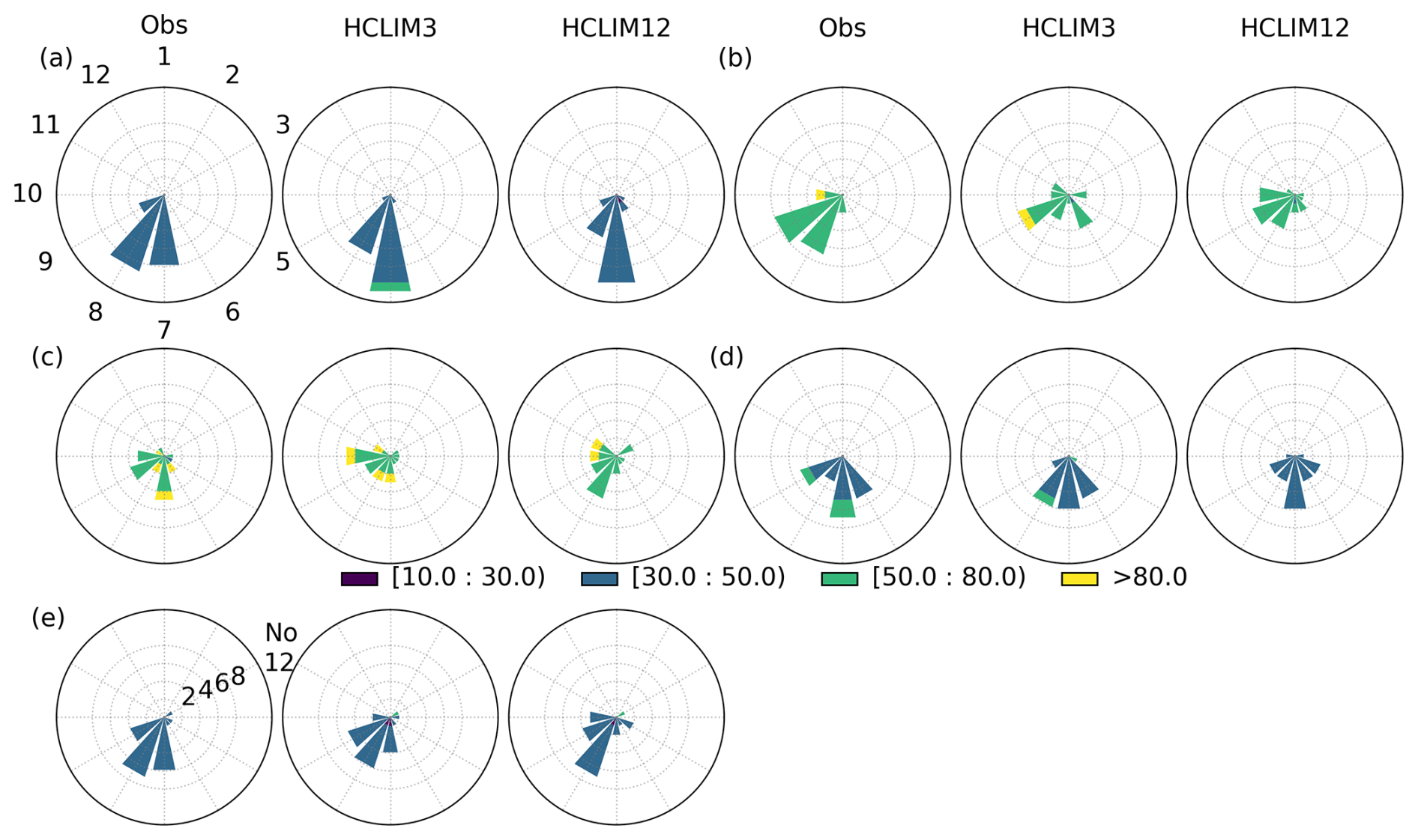
Figure 10 The seasonality of the frequency and magnitude of Rx1 d precipitation from the in situ observations, HCLIM3 and HCLIM12 during 1999–2018 over different regions: (a) east, (b) south, (c) west, (d) middle and (e) north. Radial axis represents the frequency (“no”). The color represents the magnitude of Rx1 d (mm).

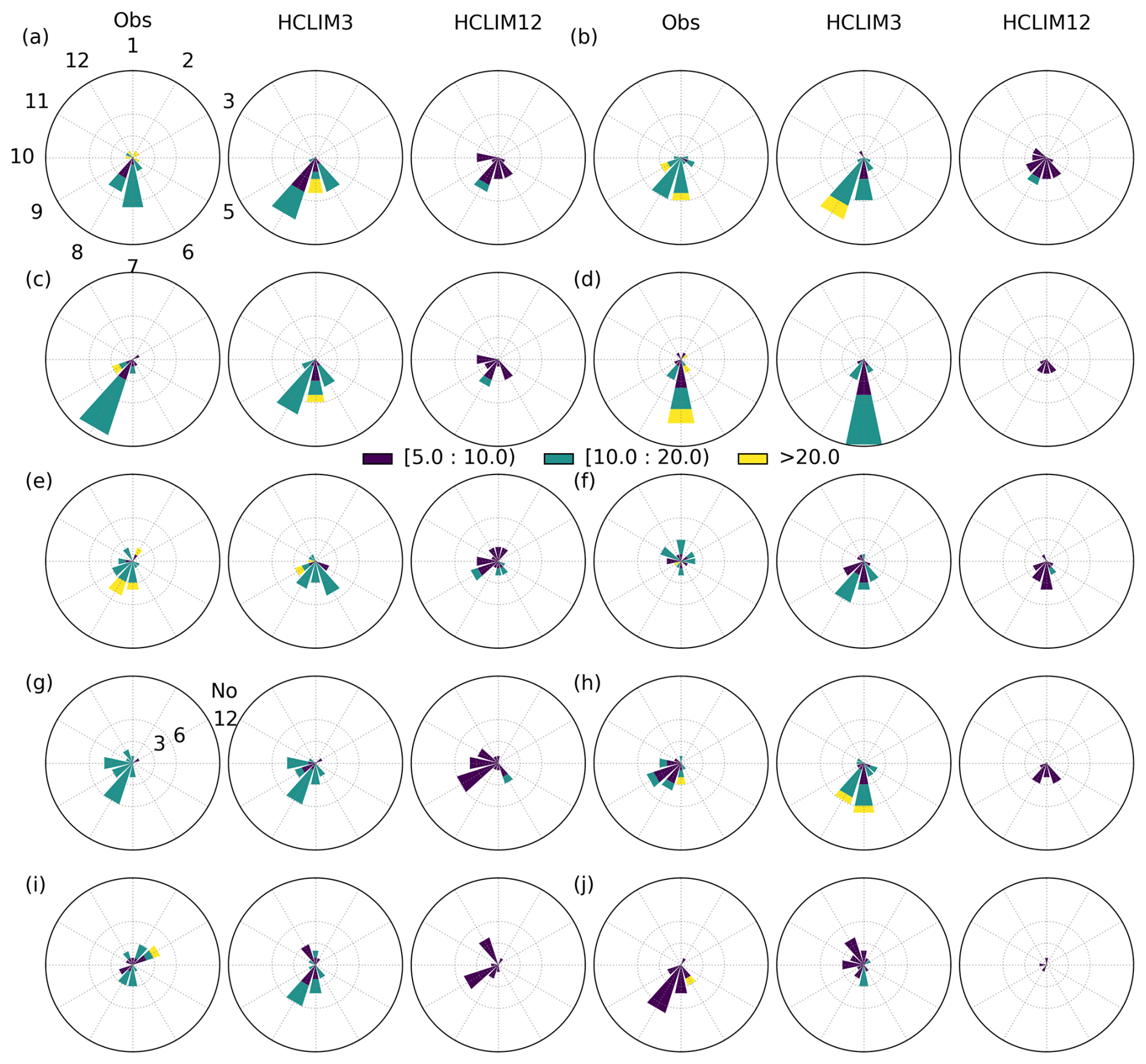
Figure 11 Seasonality of the frequency and magnitude of Rx1 h precipitation from the in situ observations, HCLIM3 and HCLIM12 during 1999–2018 at 10 rain gauge stations (Table S1), i.e., (a) Østre Toten–Apelsvoll (east), (b) Ås–Rustadskogen (east), (c) Kise in Hedmark (east), (d) Løken i Volbu (east), (e) Særheim (south), (f) Stryn–Kroken (west), (g) Fureneset (west), (h) Kvithamar (middle), (i) Tjøtta (middle) and (j) Tromsø–Holt (north). Radial axis represents the frequency (“no”). The color represents the magnitude of Rx1 h (mm).

4.5 Orographic effect on seasonal extreme precipitation

4.5.1 Seasonal Rx1 d at regional scale

The relationship of seasonal Rx1 d with elevation from SeNorge, HCLIM3 and HCLIM12 is shown in Fig. 12. Compared to HCLIM12, HCLIM3 more accurately captures the fact that there is no evident linear relationship (indicated by a coefficient of determination R² of zero) between seasonal Rx1 d and elevation, similarly to SeNorge, though it depicts a more pronounced increase with elevation than SeNorge during summer. For example, both HCLIM3 and HCLIM12 simulate a large average increase in summer Rx1 d with elevation (over 8 % km⁻¹) compared to observations, as indicated by the larger absolute slope values. Generally, SeNorge, HCLIM3 and HCLIM12 showed the weak relationship of seasonal Rx1 d with altitude.

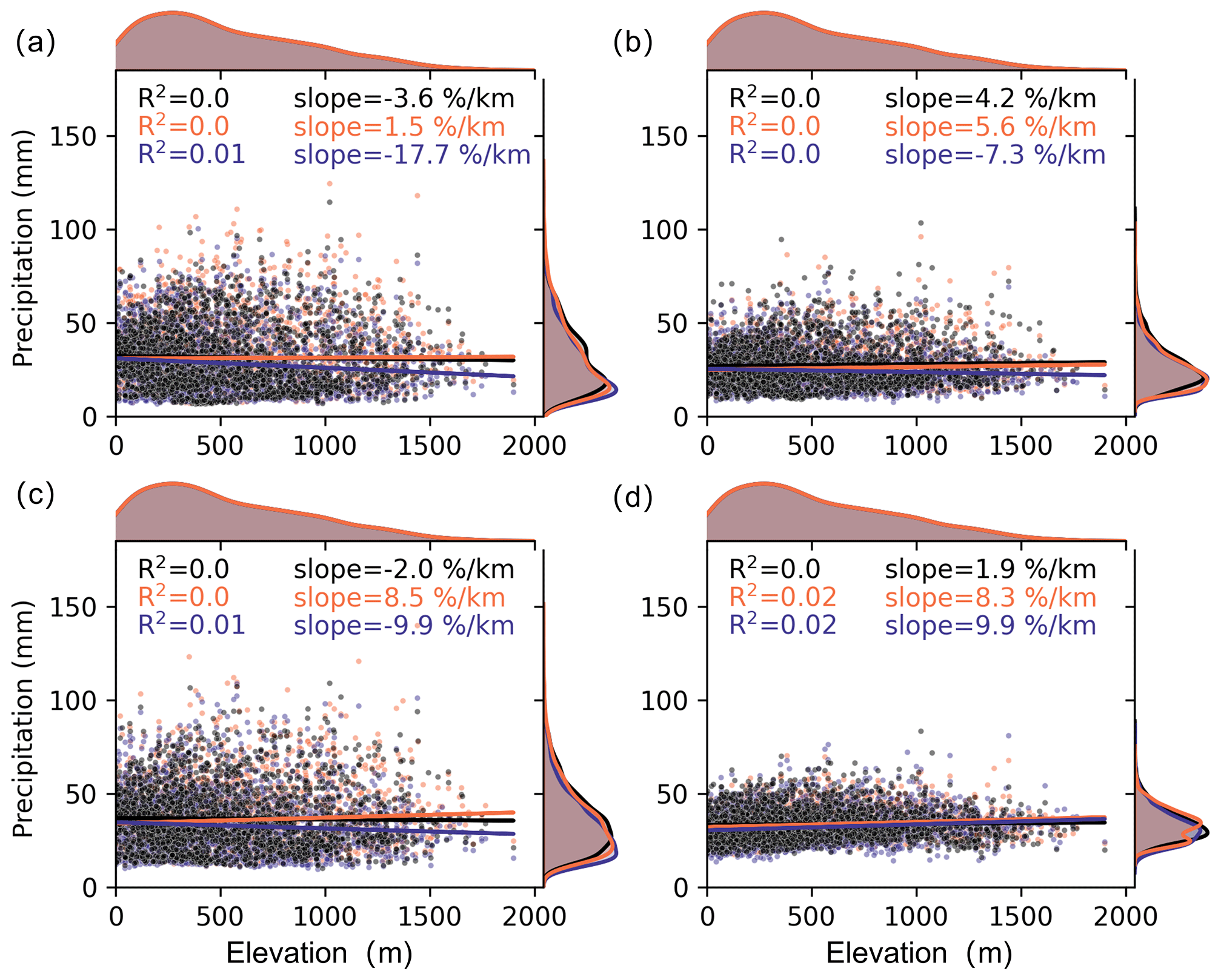
Figure 12 Relationship between elevation and Rx1 d (maximum 1 d precipitation) for (a) winter, (b) spring, (c) summer and (d) autumn, as derived from SeNorge and HCLIMs (i.e., HCLIM3 and HCLIM12) across mainland Norway during the period of 1999–2018.

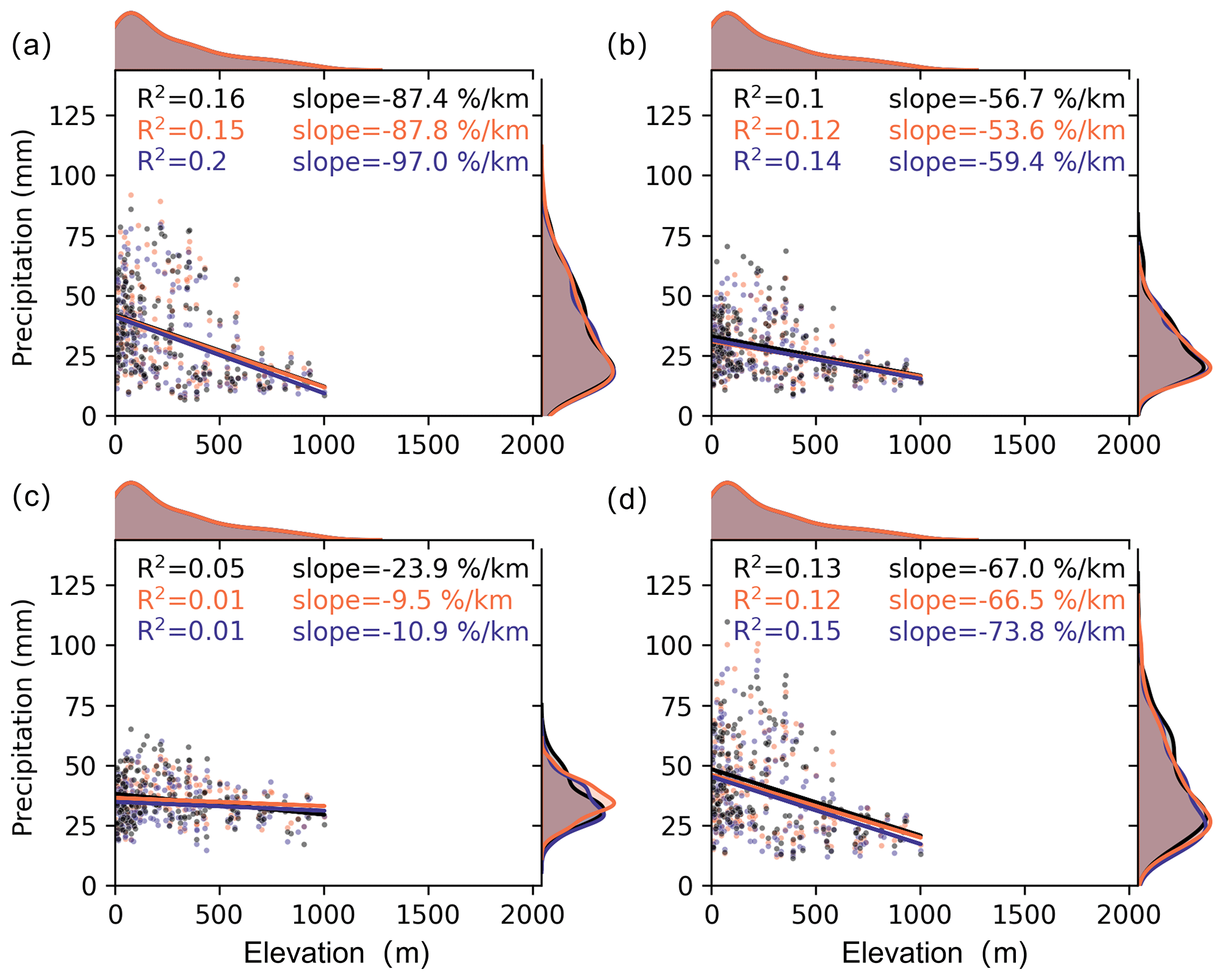
Figure 13 Relationship between elevation and Rx1 d (maximum 1 d precipitation) for (a) winter, (b) spring, (c) summer and (d) autumn based on daily in situ observations and HCLIMs (i.e., HCLIM3 and HCLIM12) across mainland Norway during the period of 1999–2018.

4.5.2 Seasonal Rx1 d at local scale

Figure 13 represents the relationship of the seasonal Rx1 d from in situ observations, HCLIM3 and HCLIM12 with elevation at the local scale. The observed reverse orographic effect, a seasonal Rx1 d decrease with elevation, is clearly depicted, with average decreases in winter, spring, summer and autumn Rx1 d of more than 87.4 % km⁻¹, 56.7 % km⁻¹, 23.9 % km⁻¹ and 67 % km⁻¹. HCLIM3 more accurately represents the observed orographic influences on Rx1 d in all seasons except summer compared to HCLIM12. Moreover, HCLIM12 displays a more pronounced decline in Rx1 d with elevation, as evidenced by a steeper slope, across all seasons, except for summer, when compared to the observations. Generally, the reverse orographic effect is shown for Rx1 d from in situ observations, HCLIM3 and HCLIM12.

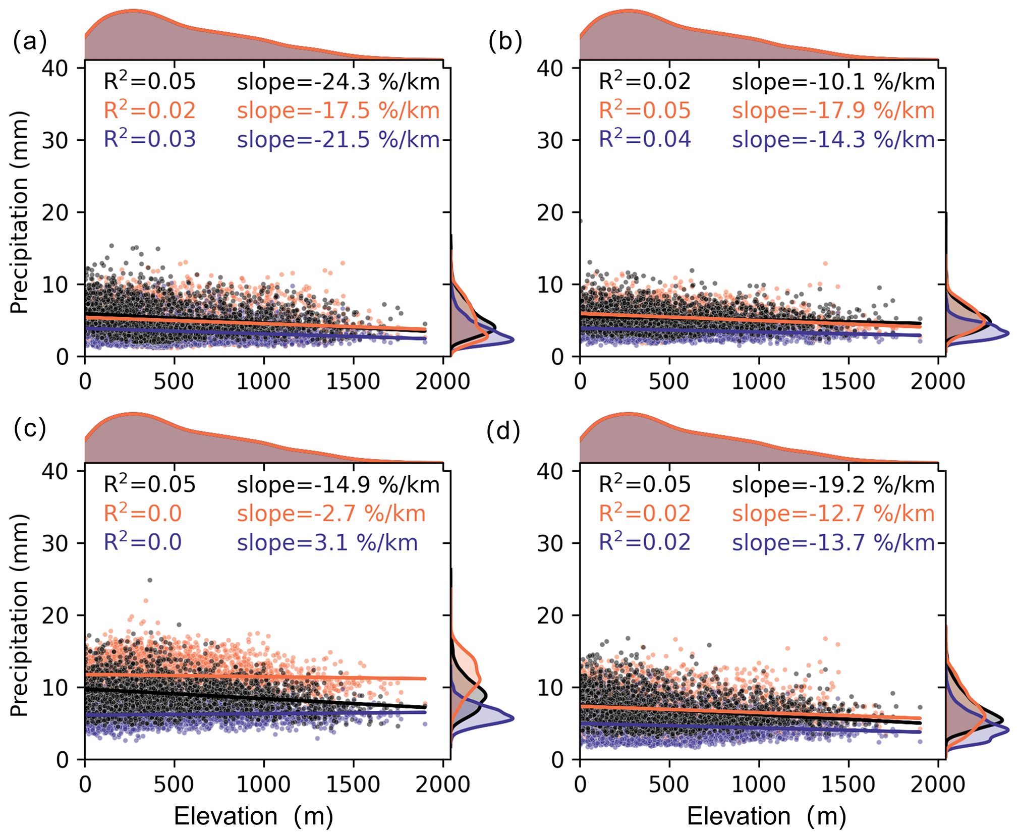
Figure 14 Relationship between elevation and Rx1 h (maximum 1 h precipitation) for (a) winter, (b) spring, (c) summer and (d) autumn, as derived from SeNorge2 and HCLIMs (i.e., HCLIM3 and HCLIM12) across mainland Norway during the period of 2010–2018.

4.5.3 Seasonal Rx1 h at regional scale

The relationship of seasonal Rx1 h with elevation from gridded observations (SeNorge2) and simulations is further explored, as shown in Fig. 14. The reverse orographic effect of SeNorge2 on Rx1 h was manifested in all seasons, with average decreases exceeding 24.3 % km⁻¹, 10.1 % km⁻¹, 14.9 % km⁻¹ and 19.2 % km⁻¹ in winter, spring, summer and autumn, respectively. Compared to HCLIM12, HCLIM3 more accurately captures the decrease in seasonal Rx1 h with elevation during winter, summer and autumn, though it still underestimates the decrease rate relative to observations. In contrast, HCLIM12 can only reflect the similar reverse orographic effect on Rx1 h with observations in spring. The density plots of Rx1 h reveal a dry bias in HCLIM12, which is particularly noticeable in summer, where it inversely correlates Rx1 h with elevation.

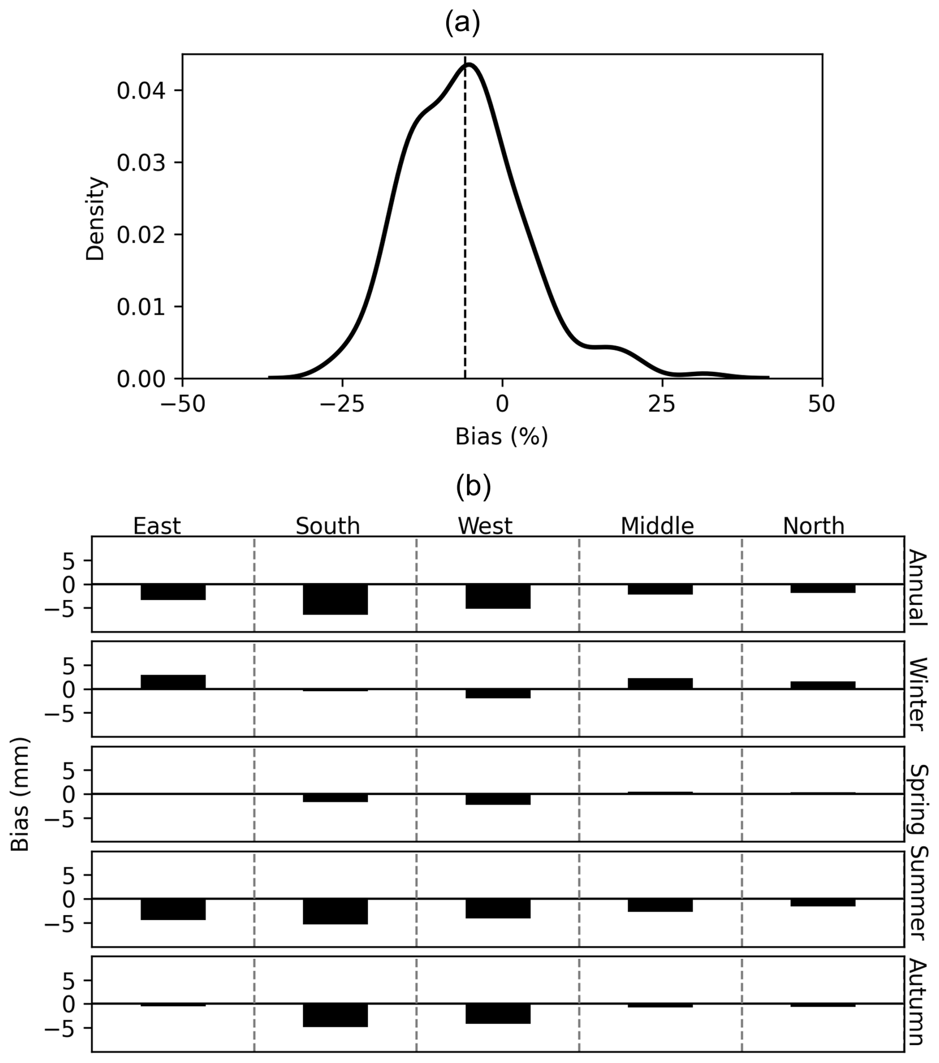
Figure 15 (a) Density distribution of bias for Rx1 d between SeNorge and daily in situ observations from 194 stations during 1999–2018; (b) the percentage difference of seasonal Rx1 d between SeNorge and daily in situ observations across the five regions. The bias is calculated as SeNorge minus daily in situ observations at each grid-point.

5 Discussion

5.1 Comparison between SeNorge and in situ observations

To further explore the uncertainty of different observation datasets in local-scale model evaluation, we investigate the bias of SeNorge's annual and seasonal Rx1 d based on daily in situ observations (see Fig. 15). Our analysis in Fig. 15a shows that SeNorge mostly underestimates the annual Rx1 d compared to in situ observations at 192 stations, with an average bias of −5.8 % and a range between −28 % and 25 %. Although SeNorge data are designed to improve hydrological simulations (Lussana et al., 2019), their dry biases still persist in most seasons and regions, especially in summer. It is noteworthy that SeNorge slightly overestimates the winter Rx1 d in the eastern, middle and northern regions. Moreover, SeNorge underestimates the return levels of Rx1 d for different return periods (e.g., 5, 10, 20 and 50 years) in all regions (Fig. S3).

The larger differences between SeNorge and in situ observations in simulating Rx1 d are manifested annually in the summer and autumn in the south and west and in the summer in the east, where SeNorge tends to underestimate Rx1 d more than the in situ observations. This discrepancy helps explain the differences between HCLIM3's performance in simulating Rx1 d in summer in the east and in autumn in the south and west at a regional scale compared to at the local scale, as shown in Figs. 2c and 5c. Generally, the difference between SeNorge and in situ observations at a daily scale is not very large, which is why, in most regions, the added value of HCLIM3 in Rx1 d at the regional scale is similar to that at the local scale. However, it should be noted that the interpolated precipitation from SeNorge may introduce uncertainties in assessing the performance of CPRCMs at the local scale due to the sparse distribution of daily and hourly rain gauges at high altitudes. In particular, for the hourly extremes at the local and regional scales, larger uncertainties should be considered due to the limited data from only 10 rain gauges at the local scale and from 9 years of data series at the regional scale. The impact of station density on the errors of gridded datasets was also highlighted by Gervais et al. (2014b), who suggested that low station density is an important source of errors in such datasets. To address these challenges and to enhance the accuracy of extreme-precipitation assessments, future studies should prioritize expanding in situ datasets and improving the spatial coverage of observational networks, especially at the 1 h timescale.

5.2 Added value of CPRCMs at the regional scale

HCLIM3 demonstrates clear advantages over HCLIM12 in capturing the annual Rx1 d in most regions. In terms of regional averages, HCLIM12 underestimates Rx1 d in most regions, except in the east, and is biased towards wetter conditions, while HCLIM3 shows relatively smaller biases in most regions, except in the east, due to improvements in microphysics and convection schemes (Lind et al., 2020).

Despite the overall better performance of HCLIM3, slightly larger biases in summer over the east, south and west may result from the model's sensitivity to convective processes and limitations in accurately resolving localized dynamics under moisture-rich and unstable atmospheric conditions. These challenges are particularly pronounced during summer, when the intensity of convective activity increases, leading to rapid atmospheric feedback and localized extremes (Poujol et al., 2021). In contrast, in winter, the southern region is mainly affected by atmospheric rivers (ARs) associated with extratropical cyclones, and HCLIM3 can better capture this feature due to its finer resolution.

In terms of annual Rx1 h, HCLIM3 outperforms HCLIM12, although it exhibits a wet bias compared to SeNorge2. HCLIM12 underestimates Rx1 h in most grids, likely due to its reliance on parameterization schemes that fail to capture extremes (Médus et al., 2022). However, HCLIM3 shows larger biases in seasonal Rx1 h in the west in all seasons, except in spring; in the eastern and middle regions, in summer, the overestimation of HCLIM3 over Norway may be attributed to the underestimation in the hourly SeNorge2 (Lussana et al., 2018). Compared with daily extremes, both HCLIM3 and HCLIM12 exhibit larger biases in simulating hourly extremes compared to daily extremes at both the annual scale and seasonal scale. It is important to note the limitations of the SeNorge2 dataset, which only spans 8 years and is interpolated from sparse hourly rain gauges.

In summary, HCLIM3 demonstrates better agreement with observations across most regions of Norway and across most seasons at the regional scale, with the exception of the east and summer. This is consistent with previous studies highlighting the advantage of convection-permitting models, especially in capturing extreme-precipitation events over complex terrain (Kendon et al., 2023; Médus et al., 2022; Lucas-Picher et al., 2021).

5.3 Added value of CPRCMs at the local scale

The analysis of local-scale convection-permitting climate models (CPRCMs) highlights their better performance in capturing precipitation extremes. HCLIM3 demonstrates notable advantages over HCLIM12, especially in terms of hourly precipitation extremes (Rx1 h). For example, HCLIM3 achieves near-zero bias for the annual Rx1 d in Norway (Fig. 5) and a relatively smaller bias for hourly extremes (Figs. 7 and 8) at all stations, while HCLIM12 consistently underestimates the return levels for hourly extremes at most stations (Fig. 8) and for daily extremes in all regions. Médus et al. (2022) also pointed out that RCMs underestimate the return levels of Rx1 h in Norway. Thomassen et al. (2023) compared the performance of HCLIM3 and HCLIM12 based on local rain gauge data in Denmark and found that HCLIM12 indeed underestimates the hourly extreme events and that HCLIM3 agrees well with observations. Despite these benefits, the added value of HCLIM3 is not uniform across all stations and seasons, struggling to capture summer daily extremes in the south and west and the return level in the east and west. However, it should also be noted that the analysis is based on data from only 10 sites, which limits the generalizability of the findings to local hourly extreme events. Further studies of hourly extreme events at more stations are needed to validate these results and to provide a more comprehensive understanding. Additionally, the uncertainties in the extreme-precipitation analysis based on the stationary GEV method with a 20-year data series should also be noted.

The added value of CPRCMs in simulating hourly precipitation extremes is more obvious at the local scale than at the regional scale. The damped extremes caused by grid-scale averaging may explain the smaller return level observed for HCLIM3 and HCLIM12 compared to station-level observations. As discussed in Sect. 5.1, this discrepancy between regional and local scales may be partly due to the inadequate density of in situ observations.

Few studies have systematically compared hourly and daily rainfall in RCMs due to the challenges in reliably simulating hourly extremes. In line with Ban et al. (2014), we find that RCMs such as HCLIM12 demonstrate reasonably good performance for daily extremes, with biases of less than 50 %. However, CPRCMs such as HCLIM3 perform better for hourly extremes. This is consistent with previous studies (Jiang et al., 2013; Thomassen et al., 2023) which showed that it is challenging to capture sub-daily extreme rainfall using RCMs with a resolution of 10 km in the southwestern United States. The better performance of CPRCMs compared to RCMs at an hourly scale is consistent with the findings by Médus et al. (2022) and Ban et al. (2014), emphasizing that the CPRCMs have significantly better sub-daily precipitation characteristics, including spatial distributions and duration–intensity characteristics. Nonetheless, further improvements in the observation networks and longer observational datasets are necessary to fully verify and realize the benefits of CPRCMs at finer spatial and temporal scales.

Comparison of regional and local extreme-precipitation seasonality confirms that HCLIM3 is able to represent the seasonality of daily extremes, although both HCLIM3 and HCLIM12 fail to capture the spring–summer events in the middle region. Moustakis et al. (2021) also highlighted the adequacy of CPRCMs (∼ 4 km) in capturing seasonality observed over the United States. In particular, we observe that HCLIM3 better represents the seasonality of hourly precipitation at the local scale. The persistent underestimation of hourly extremes by HCLIM12 may be attributed to higher uncertainty in its convective parameterization scheme or numerical uncertainties at the local scale.

5.4 Added value of CPRCMs in reproducing reverse orographic effects

An unclear relation of daily extreme precipitation with elevation was also seen from the study of Dallan et al. (2023), in which they analyzed annual daily return levels based on CPRCMs and in situ observations over an Alpine region. By comparing the relationship between the elevation and seasonal variation of extreme precipitation, HCLIM3 represents the reverse orographic effect well at regional and local scales, although there is a weak relationship between extreme precipitation and elevation at the regional scale. The reverse orographic effects on hourly and daily extremes vary with the season, indicating the influence of topography on extreme precipitation at different timescales and emphasizing the reliability of the simulation of extreme precipitation over complex terrain. Unlike Rx1 d at the regional scale, which is less affected by topography, the slope of the reverse orographic effect of daily extreme precipitation at the local scale is more clear. From a seasonal perspective, the reverse orographic effect of extreme precipitation in summer is not well captured in HCLIM3 and HCLIM12, which may be related to the intense orographically sustained convection affected by the atmospheric, aerosol conditions, local terrain slope and shadowing effects, which RCMs and CPRCMs fail to capture (Dallan et al., 2023; Poujol et al., 2021).

For hourly extremes, the reverse orography effect of the seasonal Rx1 h in this study is consistent with the reverse orographic effect of the hourly return level, as found by Dallan et al. (2023) over the Alpine region. HCLIM3 and HCLIM12 capture the reverse orography effect on seasonal Rx1 h well, especially in HCLIM3, although a stronger decrease in Rx1 h with elevation is observed from SeNorge2, except in spring. In comparison, lower Rx1 h and a weak reverse orography effect is found in HCLIM12 in all seasons. Our findings confirm the reverse orographic effect on Rx1 h, as demonstrated by Marra et al. (2021) for hourly precipitation and by Formetta et al. (2022) for the sub-hourly scale.

Furthermore, we demonstrate the reverse orographic effect for both seasonal Rx1 h and Rx1 d, which contrasts with the findings of Formetta et al. (2022), who identified an orographic enhancement for durations of approximately 8 h or longer, although a reverse orographic effect for hourly and sub-hourly durations was shown. These differences may be attributed to the combined effects of latitude, climate, altitude zones, static atmospheric or aerosol conditions, and shadowing effects (Amponsah et al., 2022; Napoli et al., 2019).

It should be noted that a simple relationship between extreme precipitation and elevation is difficult to build due to the fact that several land surface characteristics could influence the precipitation; a complex regression model should be considered to more realistically quantify the reverse orographic effect (Zhang et al., 2018) in the future. The interpolated gridded dataset and limited rain gauges over the complex orography, along with the decreasing station density at higher elevations, may also limit the reliable analysis of the reverse orographic effect. The sparsity of rain gauges and undercatch problems could also lead to the underestimation of precipitation, especially in the case of complex orography (Lussana et al., 2018, 2019; Gervais et al., 2014b).

6 Conclusions

In this study, we conducted a comprehensive evaluation of extreme-precipitation characteristics from the regional to the local scale in Norway, focusing on five distinct regions, utilizing a convection-permitting regional climate model (HCLIM3) and comparing it with its convection-parameterized regional climate model (HCLIM12) forced by ERA-Interim data during 1999–2018.

The key conclusions of this study are as follows:

• a.

  At the regional scale, HCLIM3 generally performs better than HCLIM12 in capturing Rx1 d across most regions and seasons, except for larger biases in summer over the east, south and west, as well as in the return levels of daily extremes in the east. In contrast, HCLIM12 consistently underestimates the annual daily extremes in all regions, except in the east. For hourly extremes, HCLIM3 outperforms HCLIM12 in most regions and seasons, except in summer and over the west. In general, HCLIM3 overestimates annual Rx1 h across most grid points in Norway, while HCLIM12 underestimates it.

• b.

  At the local scale, HCLIM3 also shows added value compared to HCLIM12 in capturing Rx1 d in most regions and seasons. Specifically, HCLIM3 can better capture the return levels of daily extremes in most regions, except in the west and east, and it shows smaller biases in Rx1 d across Norway for all seasons, except for summer in the south and west. Overall, HCLIM3 shows consistent benefits in capturing the daily extremes in the middle and northern regions compared with HCLIM12 at both the regional and local scales. For hourly extremes, HCLIM3 outperforms HCLIM12 in capturing the annual Rx1 h and return levels at those 10 stations.

• c.

  For the seasonality of extremes, HCLIM3 and HCLIM12 can characterize the seasonality of daily extremes well in most regions. A distinct advantage emerges with HCLIM3 for hourly extremes, with it accurately reflecting both the occurrence and intensity of these events across different seasons, while HCLIM12 tends to underestimate these aspects.

• d.

  In Norway, the effect of the preserved topography on seasonal Rx1 h and Rx1 d emerges from regional to local scales, although a weak relationship between Rx1 d and elevation is demonstrated at the regional scale. For seasonal Rx1 h, both HCLIM3 and HCLIM12 can capture the reverse orographic effect at the regional scale, but no added value is shown in HCLIM3. At the local scale, HCLIM3 provides added value in capturing the reverse orographic effect of seasonal Rx1 d in all seasons except summer.