Evaluating the effects of topography and land use change on hydrological signatures: a comparative study of two adjacent watersheds

Watershed hydrological processes are significantly influenced by land use and land cover change (LULCC) and characteristics such as topography. In economically advanced regions, coordinating land use planning and water resource management is essential for mitigating flood risks and ensuring sustainable development. This study compares the effects of terrain slope and urbanization-driven LULCC on hydrological processes in two adjacent subtropical watersheds but with distinct terrain and land cover in the Greater Bay Area (GBA) of China. We developed an integrated surface–subsurface hydrological model (ISSHM) using the Simulator for Hydrologic Unstructured Domains (SHUD) and calibrated it with data from river and groundwater monitoring stations. The calibrated model simulated hydrological processes, including surface runoff, subsurface flow, evapotranspiration (ET), and infiltration, to quantify water movement (measured in meters) and assess the impacts of slope and LULCC. Results show that slope impacts hydrological processes differently based on watershed characteristics. In mountainous areas, there are consistent high correlations between slope and annual surface runoff, infiltration, and subsurface flow across all watersheds. However, at lower elevations, the hydrological responses of steeper watersheds correlate weakly with local slope. Urbanization, marked by increased impervious surfaces, significantly raises annual surface runoff and decreases infiltration and ET, especially in steeper watersheds. In flatter watersheds, the rise in surface runoff is proportionally less than the increase in impervious areas, indicating a buffering capacity against urbanization. However, this buffering capacity diminishes with increasing annual rainfall intensity. Overall, the ISSHM provides robust analysis of LULCC effects on watershed hydrology across scales, enabling predictive approaches to optimizing urban management for sustainable development in growing cities.

1 Introduction

The effects of land use and land cover change (LULCC) and topographic variability on hydrological processes within a watershed are widely recognized as critical issues in hydrology (e.g., Bosch and Hewlett, 1982; O'Loughlin, 1986; Costa et al., 2003; Beven, 2012; Gwak and Kim, 2017; Larson et al., 2022; Sicaud et al., 2024). Urbanization has been demonstrated to significantly impact hydrological processes such as surface runoff, evapotranspiration (ET), infiltration, and subsurface flow by altering the conditions of the land surface (Olang and Fürst, 2011; Ayalew et al., 2015; Guan et al., 2015; Bai et al., 2020; Yan et al., 2023; Liang and Guan, 2024). Furthermore, it is evident that topographic characteristics have a direct influence on surface water flow paths and soil moisture, thereby affecting infiltration rates and groundwater recharge (Strahler, 1957; Hopp and McDonnell, 2009; Mirus and Loague, 2013; Smith et al., 2018; Yang et al., 2019; Zhang et al., 2022b). However, comprehending the diverse impacts of LULCC and topography on hydrological processes across disparate watersheds persists as a significant challenge due to the variability in watershed characteristics and the nonlinear nature of hydrological responses (Niehoff et al., 2002; Brath et al., 2006; Thanapakpawin et al., 2007; Du et al., 2012; Pang et al., 2022; Yin et al., 2023; Guo et al., 2023; Yan et al., 2024). In order to address these challenges, researchers employ various methodologies to dissect and quantify these effects.

Statistical analysis techniques utilizing long-term monitoring data within a watershed are commonly used to examine the effects of LULCC (Beven et al., 2008; Liu et al., 2017; Zhang et al., 2017, 2022a; Kumar et al., 2022). However, long-term changes in hydrological responses often reflect the combined impacts of climate change and LULCC, making it complicated to isolate the impacts of LULCC (Beven, 2012). The paired catchment approach is another statistical method commonly employed (Brown et al., 2005; Detty and McGuire, 2010; Yang et al., 2016; Van Loon et al., 2019), which compares monitoring data from two watersheds with different land cover but similar physical characteristics (Li et al., 2009; Shao et al., 2020). However, applying this approach in practice can be challenging due to the difficulty in identifying watersheds with similar physical characteristics. Furthermore, recent studies have indicated that LULCC-induced hydrologic alterations exhibit considerable spatial variability within watersheds, affecting upstream and downstream regions in disparate ways (Chu et al., 2010; Garg et al., 2017). In this regard, statistical analysis methods that rely on gauging datasets often lack detailed spatial resolution; therefore, employing methods that facilitate studies at finer spatial resolutions is essential for a comprehensive understanding of these variations.

Similar challenges exist when investigating the effects of topography on watershed-scale hydrological processes due to the diversity of geomorphic types and significant spatial variability within watersheds. One area where significant progress has been made is the prediction of hydrologic connectivity through topographic indices to study rainfall–runoff responses in watersheds (Jencso and McGlynn, 2011). Topographic indices have become valuable tools for predicting soil moisture and identifying saturated zones. Two successful examples are the topographic wetness index (TWI; Beven and Kirkby, 1979; Sørensen et al., 2006) and height above the nearest drainage (HAND; Nobre et al., 2011; Gao et al., 2019; Fan et al., 2019). However, some studies have reported TWI and groundwater levels have distinct relations at different locations (Detty and McGuire, 2010; Rinderer et al., 2014). Furthermore, the simulation results of HAND are highly dependent on the pattern of observed saturated zones, and it performs better at gentler watersheds (Nobre et al., 2011; Gao et al., 2019). In addition, the predictive accuracy of these indices decreases under dynamic conditions, such as at the onset of rainfall events (Seibert et al., 2003; Jarecke et al., 2021).

Recent studies have shown that hydrological models based on the Richards equation not only simulate surface–subsurface water interactions on hillslopes but also accurately describe hydrological processes under varying temporal conditions (Camporese et al., 2019). The integrated surface–subsurface hydrological model (ISSHM) is a type of Richards-equation-based fully distributed hydrological model (Shen and Phanikumar, 2010; Maxwell et al., 2014; Fatichi et al., 2016). Despite being relatively new compared to other hydrological models, the ISSHM has demonstrated significant capabilities in addressing the whole system of processes at watershed scales (Niu et al., 2017; Yu et al., 2022; Zanetti et al., 2024). By dividing the land surface into grids, such models can represent the spatial variability of hydrological processes with high spatial accuracy. They can also be solved with higher temporal accuracy by applying differential solutions to the physical governing equations. Unlike monitoring data analysis methods, ISSHMs allow hydrologists to assess the impact of specific factors by implementing designed scenarios and evaluating them across a comprehensive range of spatial and temporal scales. In recent years, ISSHMs have been proven valuable for assessing LULCC and topographic impacts at the watershed scale. For instance, Im et al. (2009) used the MIKE SHE model to show that urbanization increased total runoff by 5.5 % and overland flow by 24.8 % in a watershed. Zhang et al. (2022b) explored how topography influences subsurface flow with the HydroGeoSphere, revealing that topography plays a significant role in controlling penetration depths and stagnant zones.

While some studies have investigated the effects of LULCC and topography using the ISSHM approach, they are primarily based on the single watershed (Chu et al., 2010; Im et al., 2009; Thanapakpawin et al., 2007), hindering comparative analyses. Herein, we showcase the behavior of paired watersheds with heterogeneous patterns of both terrains and land cover that are geographically adjacent and compare them under the same subtropical climate regime. We simulate the hydrological processes of two watersheds in the Greater Bay Area (GBA), a critical economic zone in China that encompasses major cities such as Guangzhou, Shenzhen, Hong Kong SAR, and Macao SAR. According to official data, the GDP of the GBA exceeded CNY 14 trillion in 2023 (Greater Bay Area, 2024). Despite this economic success, the region faces significant challenges in achieving sustainable growth under rapid urbanization, making it an ideal case study for investigating the impacts of development on hydrological processes. For this study, we use the Simulator for Hydrologic Unstructured Domains (SHUD) as an ISSHM. It examines the influences of terrain slope and urbanization-driven LULCC on the hydrological components of surface runoff, subsurface flow, ET, and infiltration at both daily and annual scales.

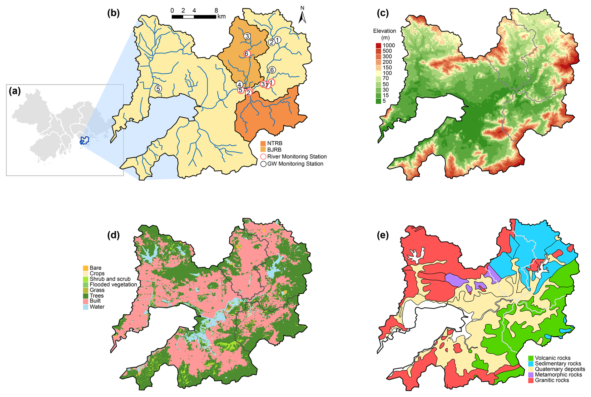
Figure 1 Location and characteristics of the Ng Tung River watershed (NTRW) and Buji River watershed (BJRW): (a) location of the Shenzhen River and Shenzhen Bay basin (SRBB) within the Greater Bay Area (GBA); (b) location of the NTRW (dark orange) and BJRW (light orange) within the SRBB (yellow), along with channels (blue), calibration river monitoring stations (numbered 1–7, red circles), and calibration groundwater monitoring stations (numbered 1–6, black circles); (c) digital elevation model (DEM) (FABDEM V1-2); (d) land cover map of 2020; and (e) geological map.

2 Study site

The study focuses on two neighboring watersheds within the Shenzhen River and Bay basin (SRBB) in the GBA – the Ng Tung River watershed (NTRW) in Hong Kong SAR and the Buji River watershed (BJRW) in Shenzhen (Fig. 1a and b). The NTRW encompasses an area of 70.7 km², while the BJRW covers 66.3 km². Situated in a subtropical region, the SRBB experiences an average annual temperature of 23.3 °C and receives a substantial amount of precipitation, averaging 1933 mm annually, with significant inter-annual variability. Notably, about 86 % of this precipitation falls during the monsoon season (April–September), with the region experiencing an average of 130 rainy days per year. The intensity of daily rainfall during this period can be significant, reaching 289 and 382 mm for the 10- and 50-year return period events, respectively.

Despite their proximity and similar climatic conditions, the NTRW and BJRW exhibit distinct differences in topography and land use patterns. The NTRW is characterized by steep slopes, with an average gradient of 12.3° and elevation variations ranging from 0.5 to 611.6 m (average elevation of 97.1 m). In contrast, the BJRW features relatively flatter terrain, with an average slope of 7.5° and elevation ranging from 0.5 to 435.3 m (average elevation of 70.6 m) (Fig. 1c). These watersheds demonstrate the rapid urbanization of Shenzhen and Hong Kong SAR since the 1980s; however, urbanization has progressed more rapidly in the BJRW. Initially, the BJRW had limited construction areas with forests predominating (Cheng et al., 2023). By 2020, built-up land in the BJRW had increased to 71 %, while in the NTRW, forests remained dominant, and built-up areas constituted 37 % of the land (Fig. 1d).

Figure 2 Model schematic of hydrological processes in the SHUD model.

3 Methodology

3.1 Hydrological model

The hydrological model employed in this study is SHUD (Shu et al., 2020), which evolved from the well-known Penn State Integrated Hydrologic Model (PIHM; Qu and Duffy, 2007; Kumar, 2009; Kumar et al., 2009). SHUD is an open-source model that incorporates a user-friendly data preprocessing toolkit, rSHUD (Shu et al., 2024), designed to simplify tasks such as grid partitioning, data integration, and model setup, addressing common challenges faced by hydrologists when working with ISSHMs. By integrating the parallel programming framework OpenMP, SHUD achieves high computational efficiency and has demonstrated superior robustness in solving problems at the watershed scale compared to PIHM, thus confirming its effectiveness in hydrological modeling (Shu et al., 2020).

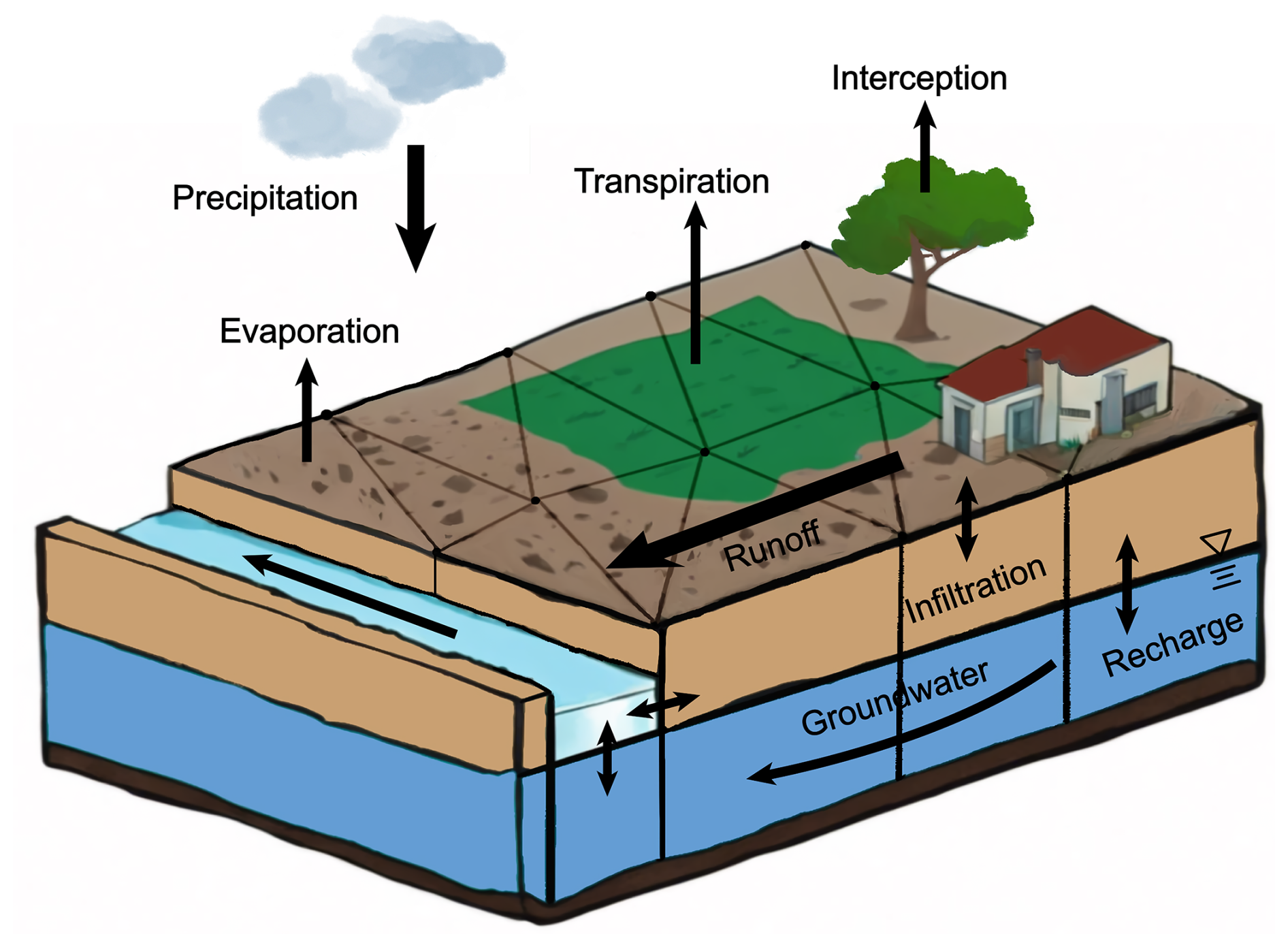
As illustrated in Fig. 2, the hydrological processes simulated by SHUD include rainfall, surface water ponding storage, surface water infiltration, surface runoff, ET, changes in unsaturated layer moisture, groundwater flow, and river flow processes. The model represents the land domain using unstructured triangular elements and trapezoid segments for the river network. Each triangular element is vertically discretized into three layers: the top layer represents the land surface, the middle layer represents the unsaturated zone, and the bottom layer represents the saturated aquifer. The model employs the finite-volume method to spatially discretize the partial differential equations of hydrological states into ordinary differential equations, enabling detailed simulation of hydrological dynamics.

For a more comprehensive understanding of the four hydrological processes analyzed in this study, we provide the relevant assumptions and computational formulas used in SHUD in Appendix A. Further details on the mathematical and algorithmic structure of SHUD are available in the referenced papers (Shu et al., 2020, 2024) and on the SHUD Book website (SHUD Book, 2024).

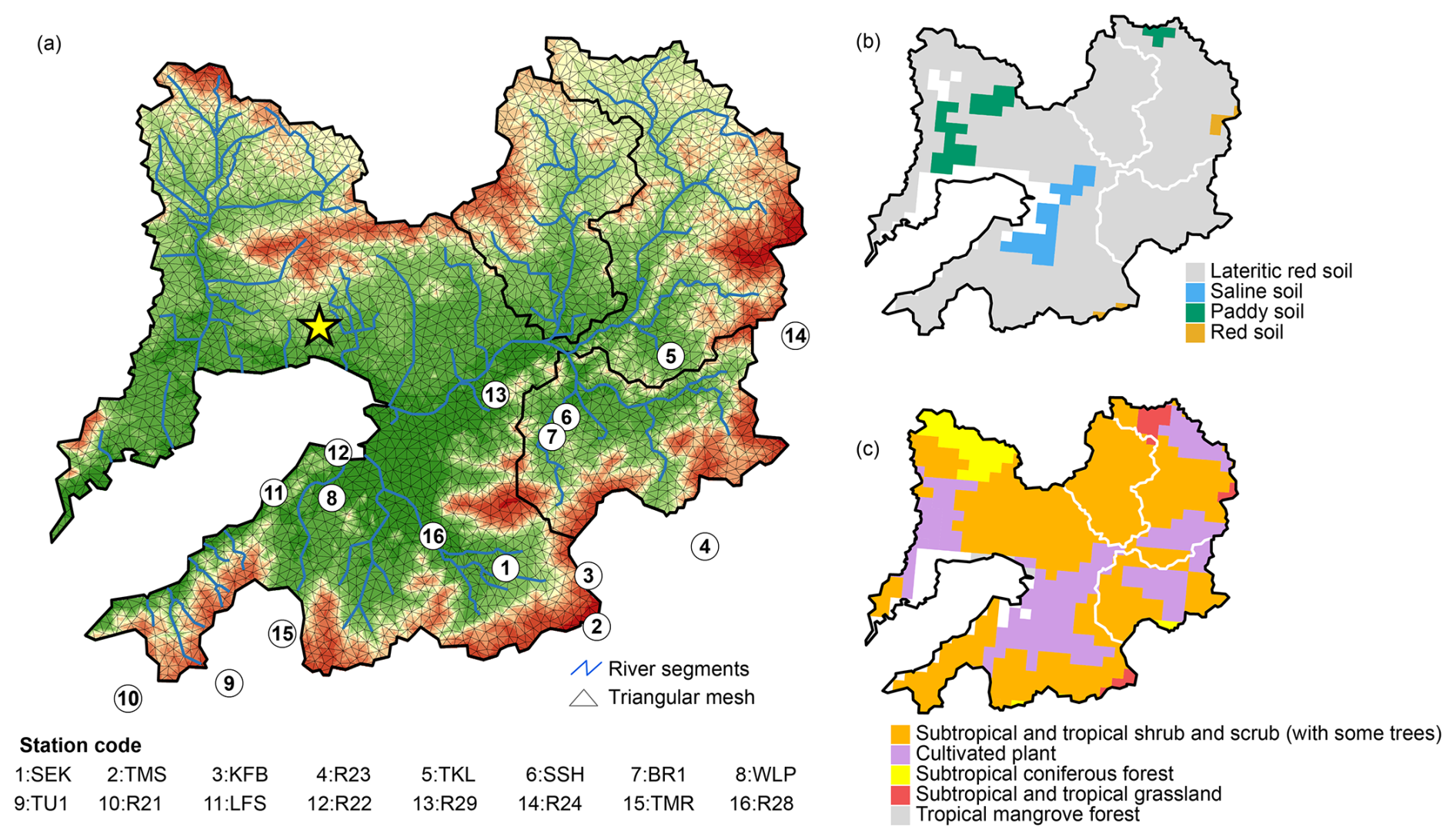
Figure 3 Map of meteorological site locations and triangular meshes of two watersheds. The black circles (numbered 1–16) represent rainfall sites located in Hong Kong SAR, and the yellow star represents the Shenzhen Meteorological Station (SMS) (a), soil map (b), and vegetation map (c).

3.2 Data collection and model setup

We set up the model domain as the entire SRBB, rather than focusing solely on its smaller two watersheds. This decision was driven by two strategic considerations. Firstly, the limited availability of monitoring data within the two watersheds necessitated a broader spatial framework to ensure a comprehensive dataset for robust hydrological analysis. Secondly, the similar characteristics of geology (Fig. 1e), soil (Fig. 3d), and vegetation (Fig. 3e) across the SRBB and its subbasins supported the feasibility of this extensive modeling approach. The SRBB, covering an area of 596 km², was discretized into 6602 triangular meshes. Specifically, the NTRW and the BJRW were represented by 819 and 793 triangular grids, respectively (Fig. 3a). In the model, the outer boundary of the SRBB was designated as a zero-flow boundary, meaning no water flows across this boundary. Additionally, the land and river boundaries along the concave boundary in the southwestern part of the basin were set as a fixed-head value, corresponding to the local sea level. This fixed-head boundary was established at 1.5 m, based on annual tidal observations from the Hong Kong Observatory (HKO). While this fixed-head approximation does not account for the precise daily tidal fluctuations, it represents a reasonable compromise for hydrological modeling purposes. Given that the two watersheds are situated significantly inland from the ocean, their hydrological processes are minimally affected by tidal variations.

The digital elevation model (DEM) for the study area was sourced from the FABDEM V1-2 dataset (Neal and Hawker, 2023) and offers a resolution of 30 m. Land cover data for 2020, with a spatial resolution of 10 m, were acquired from the Dynamic World project via Google Earth Engine (Brown et al., 2022). Data on soil types and vegetation were obtained from the Data Center for Resources and Environmental Sciences at the Chinese Academy of Sciences (RESDC, 2024), and geological information was sourced from the China Geological Survey (GeoCloud, 2024). Satellite imagery was utilized to determine river channel widths. Determining the appropriate soil depth remains a significant challenge, and as highlighted by Fan et al. (2019), weathering fractures notably influence hydrological activities. Based on the geological data from the study site, extensive weathering is noted in the mountainous regions. Consequently, the aquifer depth was modeled to vary gradually from 18 m in the upslope areas to 9 m downstream.

Table 1 Summary of collected datasets and related information.

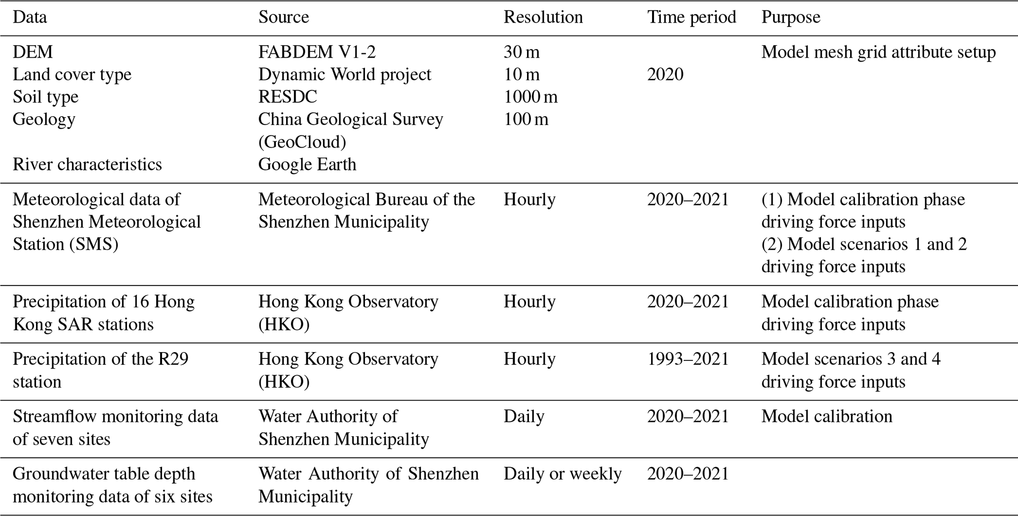
Additionally, driving force data were collected for two distinct periods. The first period, from 2020 to 2021, included hourly meteorological data from the Shenzhen Meteorological Station (SMS), provided by the Meteorological Bureau of Shenzhen Municipality. This dataset included records of precipitation, temperature, relative humidity, and wind speed. Hourly precipitation data for the same period were also gathered from 16 additional gauging sites in Hong Kong SAR, sourced from the HKO (Fig. 2a). The second period, from 1993 to 2021, involved collecting precipitation data from the R29 station via the HKO. Moreover, monitoring data of daily river discharge from seven stations and daily or weekly groundwater table depths from six stations were gathered from the Water Authority of Shenzhen Municipality for the period of 2020–2021. While urban drainage could affect river discharge in Shenzhen, river rehabilitation projects throughout 2020 (Buji Sub-district Office, 2024) helped minimize drainage network inflows. Therefore, we assume the monitored river discharge data collected during 2020–2021 can be fully attributed to terrestrial runoff intercepted along the river channels. A comprehensive summary of all datasets and related information is provided in Table 1.

3.3 Model calibration

We employed rainfall data from 17 sites covering the period from 2020 to 2021 to drive the model during the calibration process. To distribute the rainfall data effectively across all 17 sites, we utilized the Thiessen multi-polygon method, allocating the data to corresponding triangular grids. Due to limitations in data availability, meteorological parameters such as temperature, relative humidity, and wind speed were sourced solely from the SMS for the entire basin. The initial setup of the model parameters was informed by field data, the general features of the model structure, and past modeling experience. The model underwent multiple spin-up sessions using 2020 meteorological data to establish an initial condition that closely mirrors the monitoring datasets.

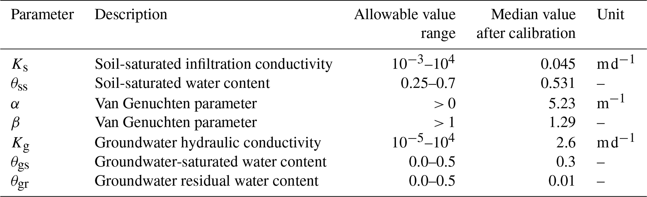
Given the heterogeneity of the basin and that the calibration target covers two types and multiple sites of monitoring datasets, effective automatic calibration becomes extremely difficult. Therefore, manual calibration methods are often preferred for ISSHMs (Shi et al., 2014; Thornton et al., 2022; Brandhorst and Neuweiler, 2023). Monitoring data from the entire period were utilized for calibration, focusing on enhancing model performance. Parameter selection was guided by prior ISSHM calibration experience, insights from the literature (Baroni et al., 2010; Song et al., 2015; Liu et al., 2020), and preliminary sensitivity analyses. Informed by these combined efforts, we identified seven critical parameters related to unsaturated zone and aquifer properties for calibration (Table 3).

As the calibrated parameters were not independent, an iterative adjustment process was required. Initially, all parameters were coarsely adjusted to match the simulation river flow with monitoring data, emphasizing trends, peak timing, and peak values, even though consistency in baseflow simulation results was not yet achieved. The next stage focused primarily on modifying aquifer-related parameters to ensure that the simulated baseflow closely matched the monitoring results. In the final stage, the groundwater table was calibrated by refining soil and aquifer parameters near the monitoring sites while minimizing significant changes to previously established parameters. These three stages were repeated until the model met our performance criteria, defined as achieving a Nash–Sutcliffe efficiency (NSE) for streamflow greater than 0.5 and simulated groundwater tables falling within acceptable observational ranges. A detailed discussion of the final calibrated parameters and results is provided in Sect. 4.1.

Figure 4 Framework for assessing the impacts of slope and LULCC on hydrological processes.

3.4 Scenario design and evaluation methods

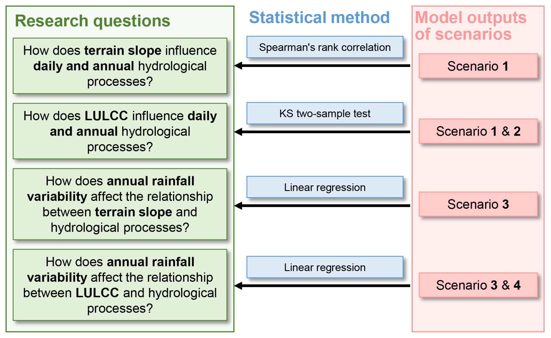
We developed four modeling scenarios differentiated by time span and land use pattern (Table 2). Scenarios 1 and 2 analyze hydrological processes at daily and annual temporal resolutions, respectively, using continuous meteorological data provided by the SMS for the years 2020–2021. These scenarios aim to determine how watershed slope and urbanization conditions influence daily and annual hydrological responses. Scenarios 3 and 4 extend the analysis to a 29-year period (1993–2021), utilizing rainfall data from the R29 station. These scenarios enrich our understanding of how annual rainfall variability influences topographic slope and LULCC in hydrological processes. The overall framework of our assessment methods is illustrated in Fig. 4, with detailed descriptions of land use pattern settings and statistical methods provided in Sect. 3.4.1 and 3.4.2, respectively.

Table 2 Designed four scenarios.

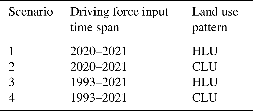
HLU, historical land use; CLU, current land use.

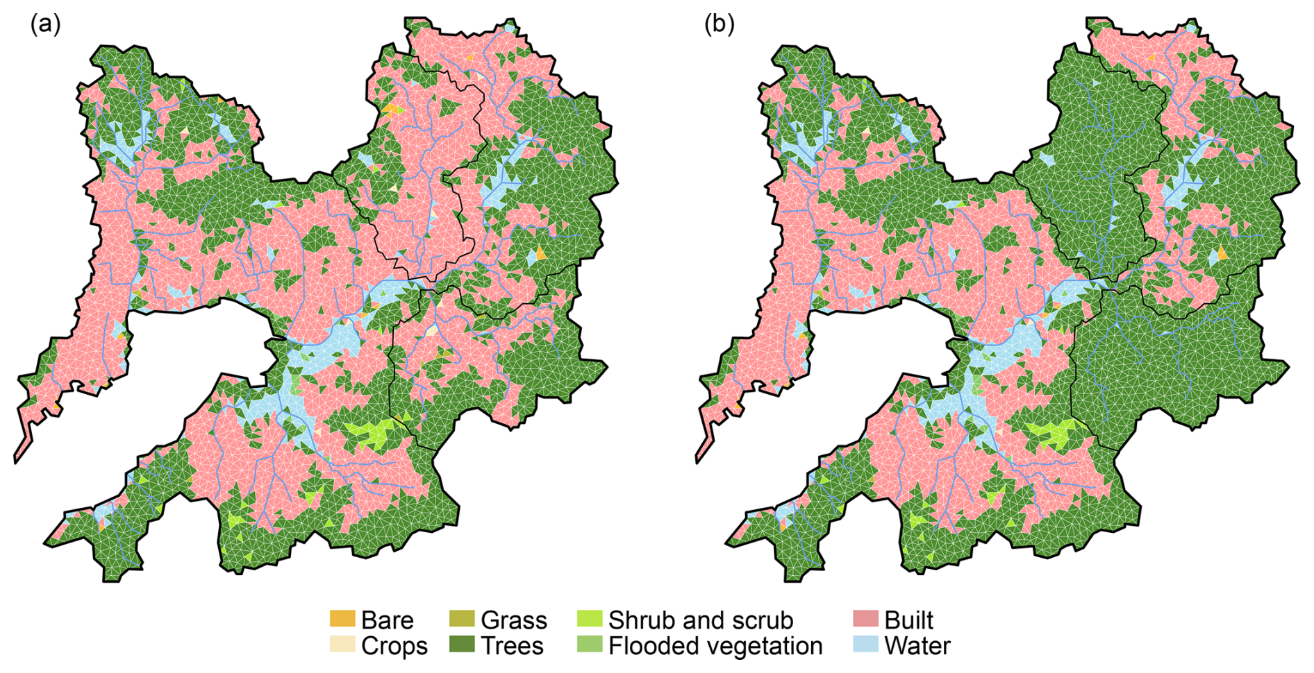
Figure 5 Model setup of land use patterns for two watersheds: (a) current land use (CLU) pattern showing the present urbanized state with extensive built-up areas (pink) mixed with other land cover types and (b) historical land use (HLU) pattern representing pre-urbanization conditions, where all built-up areas have been converted back to trees (dark green) to simulate the historical natural state.

3.4.1 Two land use patterns

Among the four scenarios, we implemented two types of land use patterns: current land use (CLU) and historical land use (HLU). The CLU pattern was derived from 2020 land use data, which were obtained from the Dynamic World project, with a spatial resolution of 10 m (Fig. 1d). The CLU pattern was generated by determining the dominant land use type based on areal coverage for each triangular mesh grid and assigning that classification to the corresponding grid (Fig. 5a). To generate the HLU pattern, we modified the CLU pattern by reclassifying all mesh grids identified as built-up land to tree cover in both watersheds, simulating pre-urbanization conditions (Fig. 5b).

Both the original raster data and our hydrological model incorporate eight land use classifications: bare land, crops, shrubs and scrubs, grassland, flooded vegetation, trees, built-up land, and water bodies (Figs. 1d and 5). Each land use type is parameterized with specific values in the model, including leaf area index (LAI), albedo, surface roughness, root zone depth, and impervious surface fraction. The impervious surface fraction is set to 94 % for built-up land, as these areas represent high-density urban development. All other land use types are assigned an impervious surface fraction of 0 %. Under the CLU pattern, built-up land comprises 37.6 % of the NTRW and 69.8 % of the BJRW. Following reclassification in the HLU pattern, the built-up land fraction becomes 0 % in both watersheds.

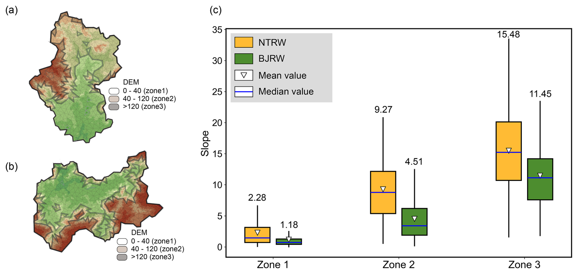
Figure 6 Elevation-based delineation of three zones in the BJRW (a) and NTRW (b), classified using DEM data as Zone 1 (0–40 m), Zone 2 (40–120 m), and Zone 3 (> 120 m). The statistical distribution of slopes within these zones is illustrated through box plots (c), with mean values labeled numerically.

3.4.2 Assessment of slope and LULCC effects

To isolate the impact of slope from LULCC effects, we analyzed slope impacts within the two watersheds exclusively under the HLU pattern. To ensure a coherent assessment of how slope influences hydrological processes, we derived slope values based on the topographical characteristics of the model instead of the original 30 m resolution DEM data. We extracted elevation values for each triangular mesh vertex from the original 30 m DEM data, re-interpolated these values to create a new raster DEM, and then calculated the average slope for each mesh grid.

For a more detailed examination of slope impacts across different spatial areas within the watersheds, we divided the watersheds into three elevation zones. First, we calculated the average elevation of each triangular mesh grid. Using the natural break method, we classified all grids into six elevation groups, with the first and second natural breakpoints at approximately 40 and 120 m. To ensure sufficient grids for reliable statistical analysis, we grouped the remaining four elevation categories into a single elevation zone. Based on these criteria, we defined three elevation zones:

• Zone 1 consists of low-elevation grids with DEM values below 40 m, primarily flat regions.

• Zone 2 includes grids with DEM values from 40 to 120 m, located at mountain foothills.

• Zone 3 comprises high-elevation grids with DEM values above 120 m.

After classification, the mean slope values for each zone are shown in Fig. 6. Since the NTRW terrain is generally steeper, the average slope value for each zone is greater in NTRW than in BJRW.

The statistical method used to examine the influence of slope on hydrological responses is Spearman's rank correlation method (Seibert et al., 2003; Hauke and Kossowski, 2011). To analyze how annual rainfall variability affects the correlation between topographic slope and hydrological processes, we developed a simple linear regression model (Appendix B).

To evaluate the impacts of LULCC, we compared hydrological outputs between CLU and HLU patterns. We employed the Kolmogorov–Smirnov (KS) two-sample test (Lilliefors, 1967) to assess the statistical significance of LULCC-induced changes in hydrological responses. To investigate how annual rainfall variability influences the relationship between LULCC and hydrological processes, we developed a simple linear regression model, following the slope assessment method (detailed in Appendix B).

Table 3 Refined parameters for the watershed after calibration.

4 Results and discussion

4.1 Model performance

Due to spatial heterogeneity within the watersheds, the calibrated values for each parameter are formed as a matrix. For clarity, only the median values are displayed (Table 3). The first four parameters, K_s, θ_ss, α, and β, are primarily associated with the vadose zone and significantly influence the hydraulic processes in the soil layer. The last three parameters, K_g, θ_gs, and θ_gr, govern the hydraulic processes in the aquifer layer. All these parameters fall within reasonable ranges, as supported by previous studies (Das, 1990; Freeze and Cherry, 1979; Bear, 1988; Van Genuchten, 1980).

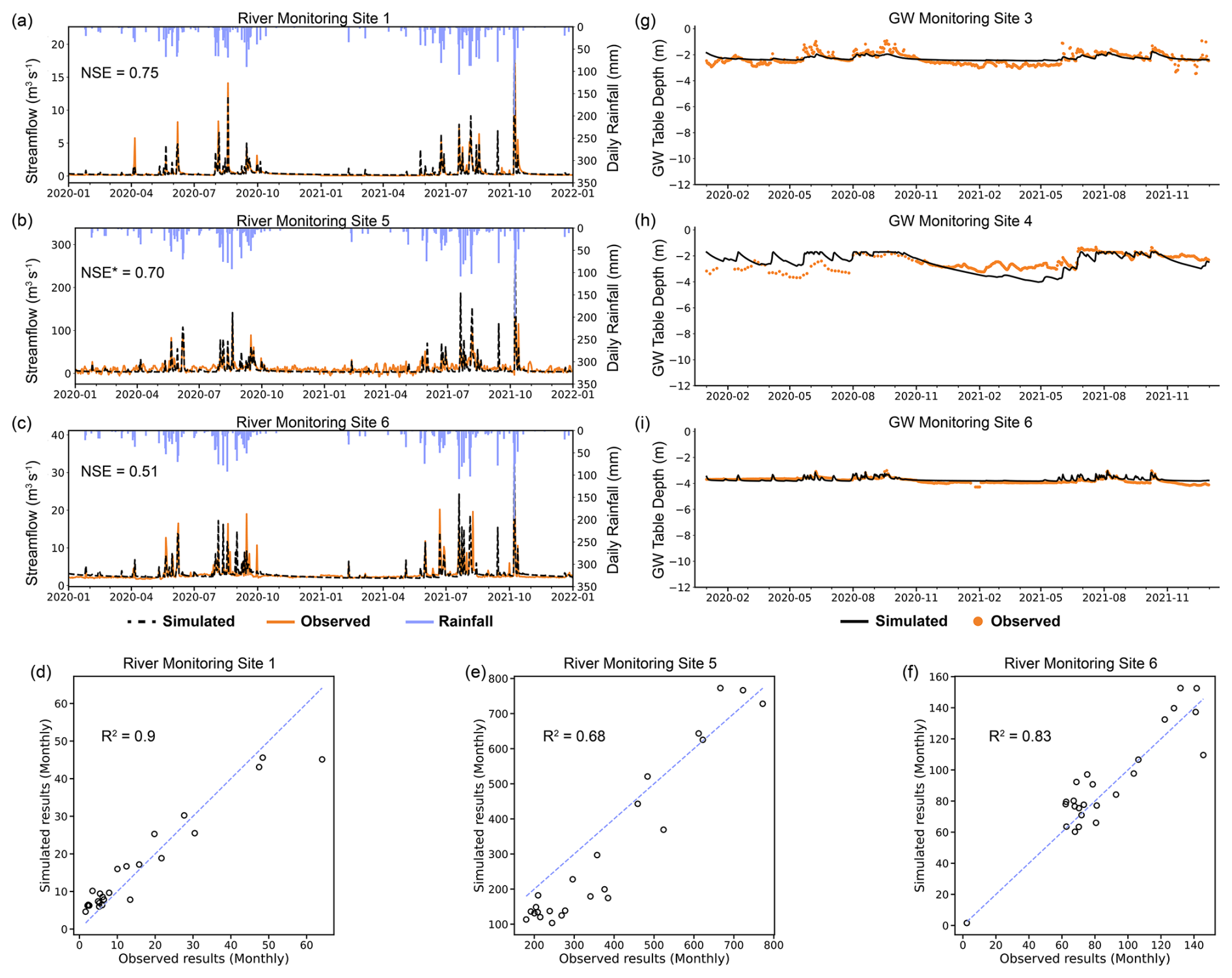
Figure 7 Calibration performance of SHUD model across daily river discharge in the river monitoring sites 1, 5, and 6 (a–c) and monthly river discharge in the river monitoring sites 1, 5, and 6 (d–f), as well as groundwater table depth in the groundwater monitoring sites 3, 4, and 6 (g–i).

Figure 7a–c display the hydrographs of daily simulated and observed streamflow at various river gauging stations within the BJRW (Site 6; Fig. 7c), upstream of the watersheds (Site 1; Fig. 7a) and downstream of the watersheds (Site 2; Fig. 7b), respectively. The NSE indices, computed for the entire simulation period, demonstrate satisfactory model performance, except for Site 2, where the observed dataset shows daily fluctuations in river flow during rain-free periods due to tidal influences. Therefore, for such sites, we specifically calibrated the discharge during rainy days and calculated the NSE index using data from those days. The simulation results exhibit satisfactory performance, with NSE indices greater than 0.5, indicating reasonable accuracy in streamflow predictions.

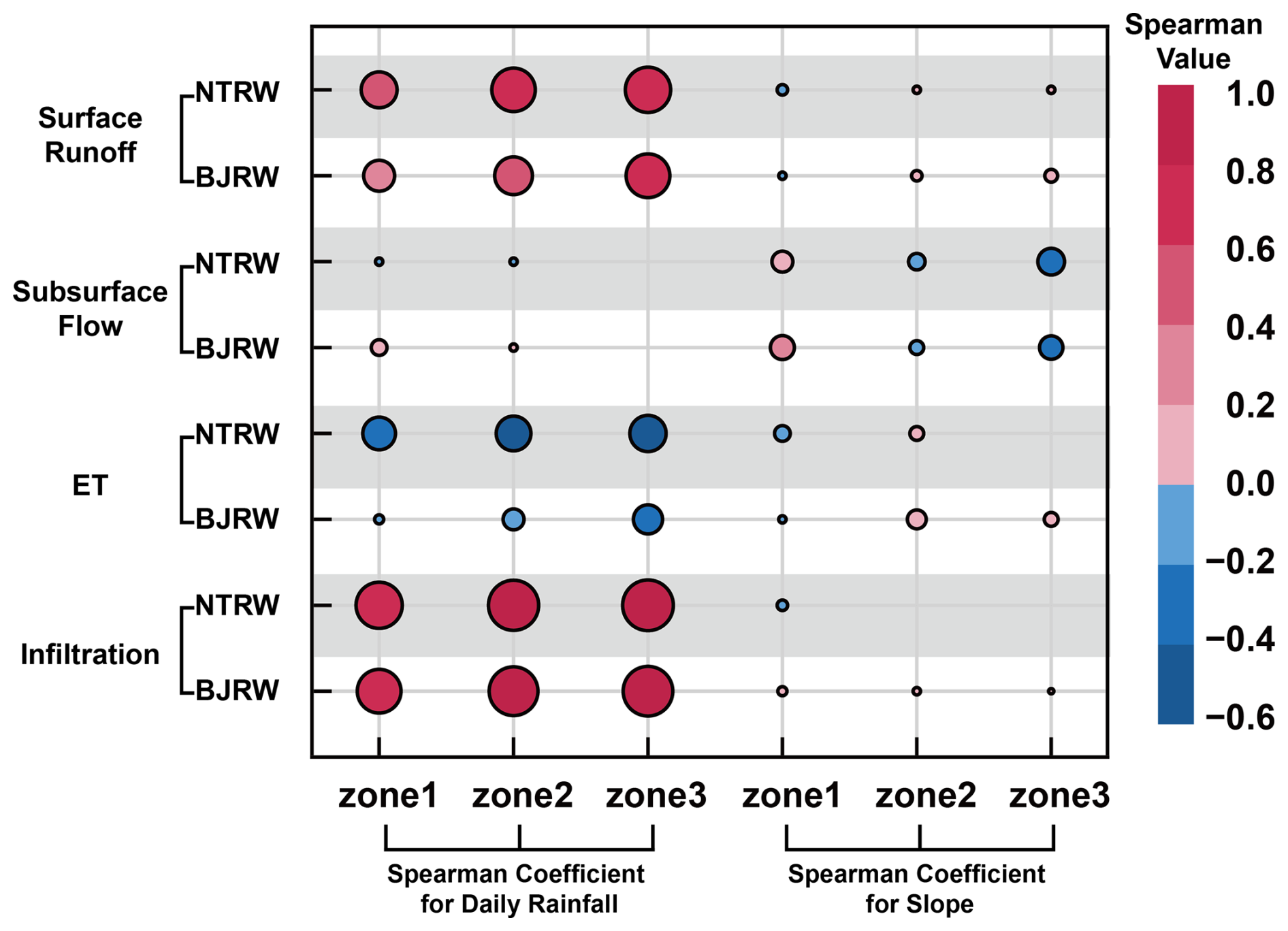
Figure 8 Comparative analysis of slope and daily rainfall influence on four hydrological variables. The marker size denotes the absolute value of the Spearman correlation coefficients, while the marker color indicates the direction of the relationship between slope or rainfall and the four model outputs. Generally, darker red represents a stronger positive correlation, whereas darker blue denotes a stronger negative correlation.

Furthermore, the monthly calibration results reinforce the robust performance of the calibrated model, exhibiting R² values exceeding 0.6 (Fig. 7d–f; Moriasi et al., 2007). This strong correlation suggests consistent and reliable model behavior over a longer timescale. Figure 7g–i present the comparisons between the simulated and observed groundwater data. It is challenging to evaluate the assessment indices of groundwater calibration for such long durations. However, our calibration outcomes indicate a marked concordance between the model outputs and observed data trends, and the modeled groundwater table depth closely aligns with the measured depths, underscoring the model's accuracy in reflecting actual groundwater conditions. Overall, the model exhibits satisfactory performance on both surface and subsurface water flows. Additional sites' calibration results are available in Fig. C1.

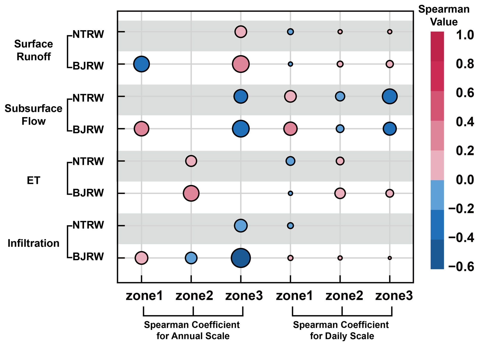
Figure 9 Comparison of hydrological responses to slope variability on annual and daily scales in the NTRW and BJRW.

4.2 Daily- and annual-scale hydrological responses

4.3 Stronger correlation between slope and daily subsurface flow

Figure 8 depicts the Spearman correlation test between four hydrological processes and terrain slope on a daily scale (i.e., on the rainy days), with all depicted markers being statistically significant (p value ≤ 0.05). The analysis primarily emphasizes slope but also explores the influence of daily rainfall to provide additional insights. The correlation analysis between daily rainfall and hydrological processes reveals distinct patterns of influence. Infiltration and surface runoff demonstrate the strongest response to rainfall amounts, with correlation coefficients ranging from −0.6 to 1, while their correlation with terrain slope remains relatively weak (between −0.2 and 0.2) in all zones of the two watersheds. ET emerges as the third most strongly correlated process with rainfall. Notably, subsurface flow exhibits a different pattern, showing a stronger correlation with local slope (coefficients between −0.4 and 0.2) than with rainfall amounts (coefficients between −0.2 and 0.2) during rainy days. This finding aligns with existing literature, highlighting the critical role of topography in influencing groundwater dynamics during rainfall events (Hopp and McDonnell, 2009; Detty and McGuire, 2010; Jencso and McGlynn, 2011; Singh et al., 2021). In both watersheds, the relationship between slope and subsurface flow varies with elevation, revealing a complex interplay between topography and groundwater dynamics. A negative correlation exists between slope and subsurface flow in Zones 2 and 3, while a positive correlation is observed in Zone 1. This indicates that in the low-elevation Zone 1, as slope increases, subsurface outflow also increases, while in the mid- and high-elevation Zones 2 and 3, as slope increases, subsurface flow decreases. In low-elevation areas, the groundwater table is typically shallow, and the soil is relatively saturated. Under these conditions, increasing slope significantly enhances the lateral hydraulic gradient, thereby facilitating downslope groundwater flow. In mid- to high-elevation areas, the groundwater table is generally deeper. Steeper slopes tend to boost surface runoff, reducing infiltration and diminishing groundwater recharge. Consequently, a negative correlation arises between slope and groundwater outflow in these higher-elevation zones.

4.3.1 Faint slope–flow relationship in the NTRW's lower zone

Figure 9 presents the comparative results of terrain slope at daily and annual scales. The findings suggest that slope has a more pronounced relationship with annual surface runoff, subsurface flow, and infiltration at higher elevations (Zone 3) compared to those at daily scales. This pattern emphasizes the pivotal role of slope in redistributing water post-rainfall events in mountainous regions. Seibert et al. (2003) and Rinderer et al. (2014) noted that topographic indices more accurately reflect hydrological responses under steady-state conditions. Specifically, Rinderer et al. (2014) reported from their analysis of data from 51 groundwater wells in a Swiss catchment that the ability of the TWI to predict water table distributions diminishes under unsteady conditions. These findings from previous studies align with our results, where the stronger correlations observed at annual (more steady-state) scales compared to daily (unsteady) scales suggest that topographic controls on hydrological processes are more pronounced and predictable over longer time periods when the system approaches steady-state conditions.

In mid-elevation regions (Zone 2), the most significant finding is the positive correlation between annual ET and local slope. This relationship suggests that steeper slopes in mid-elevation zones exhibit higher annual ET amounts. Spearman correlation analysis (results not shown) between slope and annual average soil moisture across Zone 2 grids revealed a correlation coefficient of 0.25 (p value < 0.05), indicating a positive correlation. Areas with steeper slopes have higher soil moisture, potentially contributing to higher ET amounts. Lee and Kim (2022) reported similar findings in the Sulmachun watershed, South Korea, where they observed a positive correlation between surface (10 cm) soil moisture and surface slope through April–December monitoring.

Analysis of annual flow processes at lower elevations (Zone 1) reveals a strong correlation between terrain slope and hydrological behavior in the gently sloping BJRW. However, this correlation is markedly weak in the steeper NTRW. This difference can be explained by the rapid water movement in steeper watersheds (Fan et al., 2019; Singh et al., 2021), where hydrological processes at lower elevations are dominated by swift upstream inflows rather than local topographic features. Conversely, watersheds with gentler slopes experience slower flow processes, allowing local topography at lower elevations to persistently influence water flow pathways.

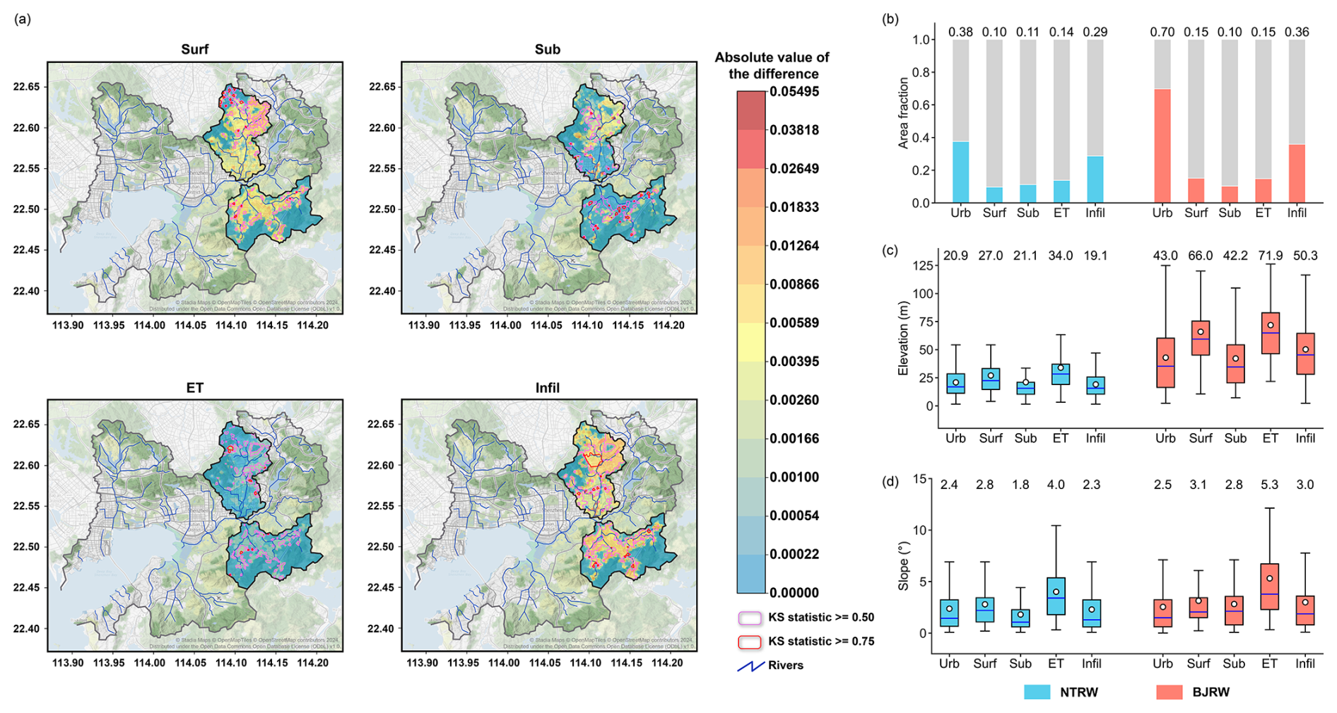
Figure 10 Spatial analysis of urbanization impacts on hydrological processes in the NTRW and BJRW. (a) Spatial distribution of KS statistics and absolute differences between the first and second scenarios for four hydrological processes: surface runoff (Surf), subsurface flow (Sub), evapotranspiration (ET), and infiltration (Infil). The color scale represents the absolute value of the differences, with areas outlined in pink and red indicating KS statistics > 0.5 and > 0.75, respectively. (b) Percentage of significantly affected areas (KS > 0.5) for each hydrological process. (c) Elevation distribution and (d) slope distribution of significantly affected areas, with the blue and red boxes representing the NTRW and BJRW, respectively. Box plots show the median (horizontal line), the 25th and 75th percentiles (box boundaries), and the mean value (white dot with corresponding text above each box).

The comparison between daily and annual scales reveals distinct temporal characteristics in slope and hydrological process relationships. At the daily scale, surface processes show immediate responses to rainfall with weak slope correlations, while subsurface flow exhibits stronger topographic control. However, at the annual scale, the influence of slope becomes more pronounced across all hydrological processes, particularly in higher elevations. This scale-dependent behavior suggests that while local topography may have a limited immediate impact on daily hydrological processes, its cumulative effects become increasingly significant over longer time periods. This temporal distinction is particularly evident in watersheds with different slope gradients. In steep watersheds, lower-elevation regions show weak correlation with local slope, while in watersheds with gentle slopes, local topographic features have a more persistent influence on flow pathways. These findings highlight the importance of considering both temporal scales and watershed characteristics in understanding topographic controls on hydrological processes.

4.3.2 Dominant impact of LULCC on daily infiltration

Figure 10a illustrates the absolute mean differences in rainy-day hydrological outputs between the HLU and CLU patterns for each grid cell. Employing the KS statistic test, significant alterations in the cumulative distribution function (CDF) of daily hydrologic outputs were identified, highlighting the substantial impacts of LULCC. Among the hydrological processes examined, daily infiltration exhibits the most pronounced and widespread differences, underscoring the dominant influence of LULCC. When considering only absolute mean differences, surface runoff is identified as the second most influenced processes. This finding aligns with the results of Chu et al. (2010) and Diem et al. (2021), which underscore the extensive impact of urbanization on surface runoff through changes in infiltration.

Regions with a KS statistic greater than 0.5 are considered to be significantly affected by urbanization. The spatial statistical characteristics of these regions for four hydrological processes are analyzed in Fig. 10b–d. Infiltration exhibits the most extensive spatial impact, whereas changes in surface runoff, subsurface flow, and ET are confined to more limited areas (Fig. 10b). Considering the elevation variations, the influenced surface runoff and ET regions are more significant at higher elevations, while the most influenced subsurface flows are limited to lower-elevation regions (Fig. 10c). Notably, areas with significant ET changes are characterized by steeper slopes (Fig. 10d). Figure 10 demonstrates that hydrological processes most influenced by urbanization are not uniform but rather concentrated in specific regions.

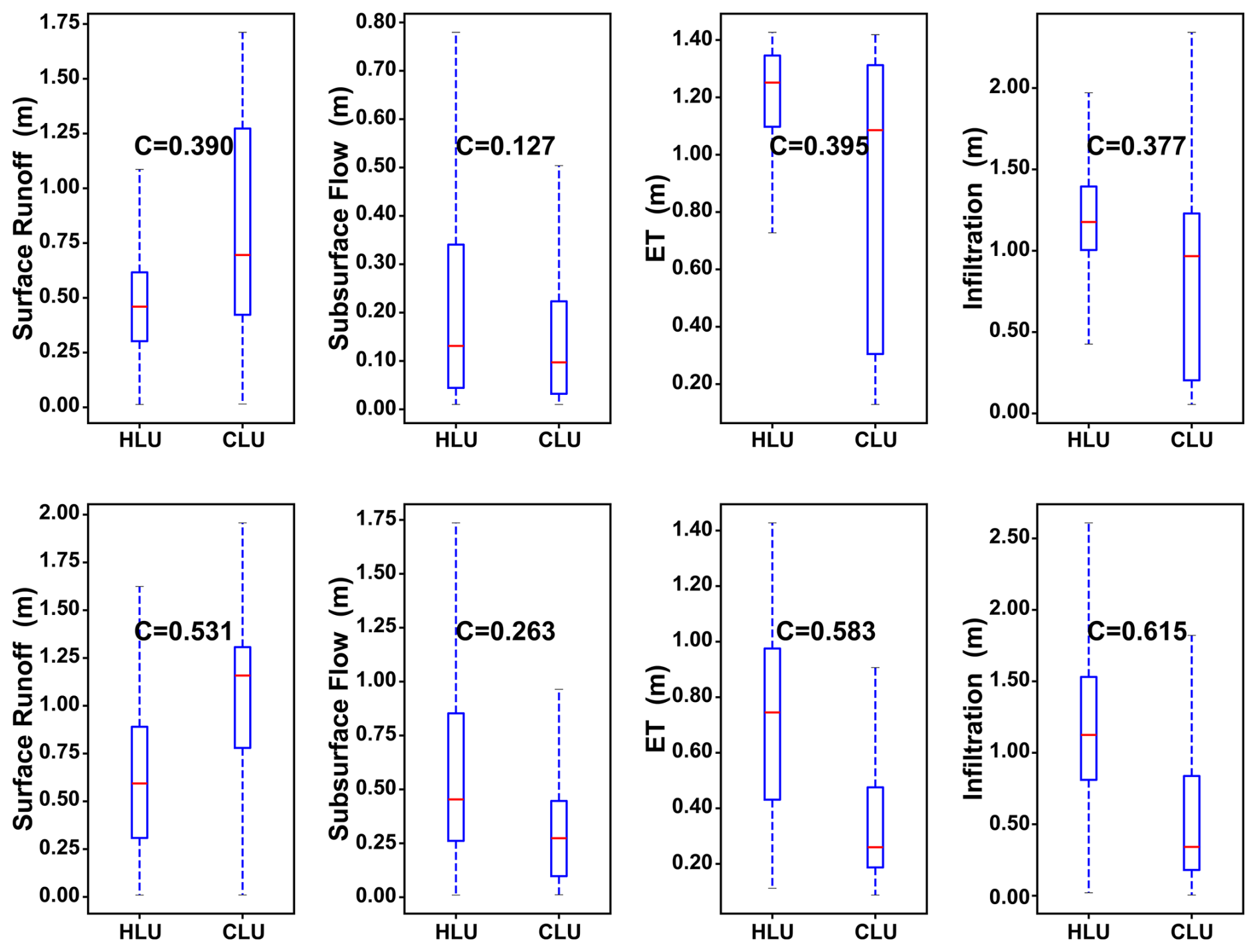
Figure 11 Box plots delineating the impacts of LULCC on the four annual outputs across all meshes within each watershed. The comparison contrasts the outcomes under the HLU and CLU patterns. The top row displays the results of the NTRW, while the second row displays the results of the BJRW. KS test values (C) are annotated, and all p values are less than 0.05.

4.3.3 NTRW shows more sensitivity to LULCC

The KS test indicates statistically significant changes in all four hydrological outputs at an annual scale after urbanization, with all p values below 0.05 (Fig. 11). The results depict an increase in annual surface runoff and reductions in subsurface flow, ET, and infiltration following urbanization. This aligns with findings from Shao et al. (2020), who used a process-based hydrological model to examine the response of surface runoff to LULCC in two adjacent watersheds in Texas, USA. They reported that urbanization leads to increased runoff, a finding consistent with our results. Furthermore, the KS test results reveal relative consistency within each watershed for surface runoff, ET, and infiltration values. Specifically, in the NTRW, the KS values for surface runoff, ET, and infiltration are recorded at 0.39, 0.395, and 0.377, respectively. The corresponding values in the BJRW are 0.531, 0.583, and 0.615. However, subsurface flow shows lower KS values of 0.127 in the NTRW and 0.263 in the BJRW, suggesting that urbanization has a lower impact on the annual subsurface flow process.

Although urbanized land accounts for 69.8 % of the land cover change in the BJRW, resulting in more pronounced responses in the four hydrological processes compared to the NTRW (where urbanized land comprises only 37.6 % of the change), it is noteworthy that per unit of urbanized area, the flatter watershed demonstrates a greater capacity to mitigate the effects of LULCC. This is evidenced by the KS values for surface hydrological processes in the BJRW (ranging from 0.531 to 0.615) being lower than the proportion of urbanized land change (0.698). In the NTRW, the KS values for surface hydrological processes (ranging from 0.377 to 0.395) are slightly higher than the proportion of urbanized land change (0.376). This observation is supported by Zhou et al. (2015), who noted that flatter terrains tend to absorb changes more effectively due to prolonged water–soil contact times, which enhance infiltration and storage capacities. This capacity may help mitigate the more severe hydrological alterations typically associated with extensive urbanization.

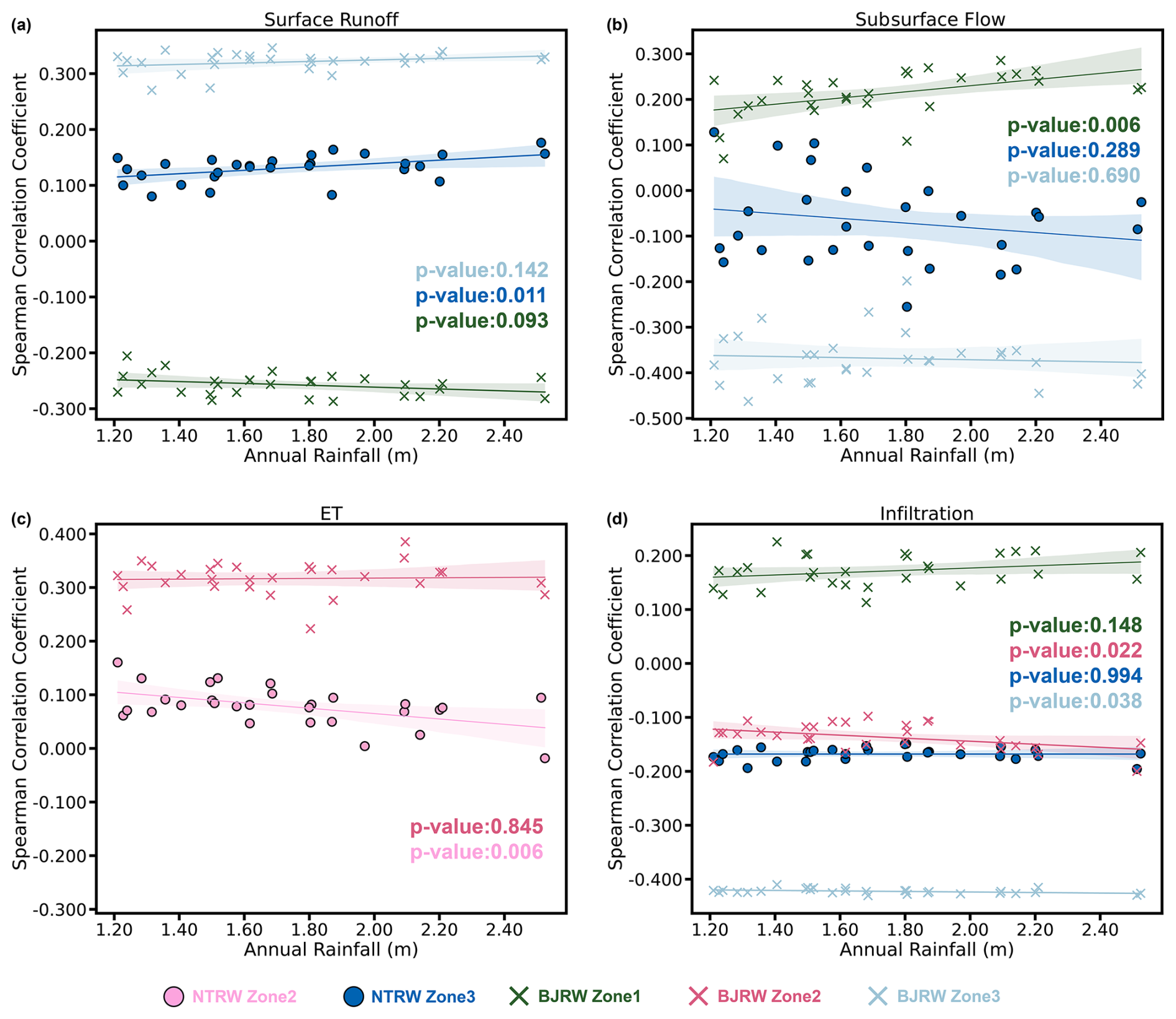
Figure 12 Scatter plots of Spearman statistic values of slope and four model outputs under 29 years of different annual rainfall amounts, with statistical significance levels indicated by the p values in the plots. Shaded areas indicate 95 % confidence intervals. Regression equations for surface runoff at (a) the NTRB in Zone 3 ($y=\mathrm{0.03}x+\mathrm{0.08}$) and the BJRB in Zone 1 ($y=-\mathrm{0.02}x-\mathrm{0.23}$) and Zone 3 ($y=\mathrm{0.01}x+\mathrm{0.3}$). Subsurface flow at (b) the NTRB in Zone 3 ($y=-\mathrm{0.05}x+\mathrm{0.02}$) and the BJRB in Zone 1 ($y=\mathrm{0.07}x+\mathrm{0.09}$) and Zone 3 ($y=-\mathrm{0.01}x-\mathrm{0.35}$). ET at (c) the NTRB in Zone 2 ($y=-\mathrm{0.05}x+\mathrm{0.16}$) and the BJRB in Zone 2 ($y=\mathrm{0.003}x+\mathrm{0.31}$). Infiltration at (d) the NTRB in Zone 3 ($y=\mathrm{0.000}x-\mathrm{0.17}$) and the BJRB in Zone 1 ($y=\mathrm{0.02}x+\mathrm{0.13}$), Zone 2 ($y=-\mathrm{0.03}x-\mathrm{0.09}$), and Zone 3 ($y=-\mathrm{0.005}x-\mathrm{0.41}$).

4.4 Variations with different annual rainfall amounts

4.4.1 Rainfall intensifies subsurface flow–slope relationship in the BJRW's lower zone

Figure 12 presents scatter plots and regression equations that analyze the correlation between annual precipitation and Spearman statistic values from 1993 to 2021, highlighting outcomes that are statistically significant (p value ≤ 0.05), as identified in Sect. 4.3.1. The analysis shows minimal changes in Spearman statistic values across most study areas; however, a notable variation was observed in subsurface flow within Zone 1 of the BJRW, where a coefficient of 0.07 indicates that each 100 mm increase in annual precipitation enhances the correlation between slope and subsurface flow by 0.007. This change corresponds to a shift in the Spearman coefficient from 0.174 to 0.258 as annual rainfall increases from 1200 to 2400 mm. This observation is supported by findings from Zhang et al. (2022b), who reported that under scenarios of higher precipitation and greater hydraulic conductivity, the extent and permeation depth of the saturated zones beneath mountains exhibit a stronger correlation with the terrain. This effect is likely due to increased precipitation levels raising the water table at lower elevations, thus enhancing the relationship between slope and subsurface flow.

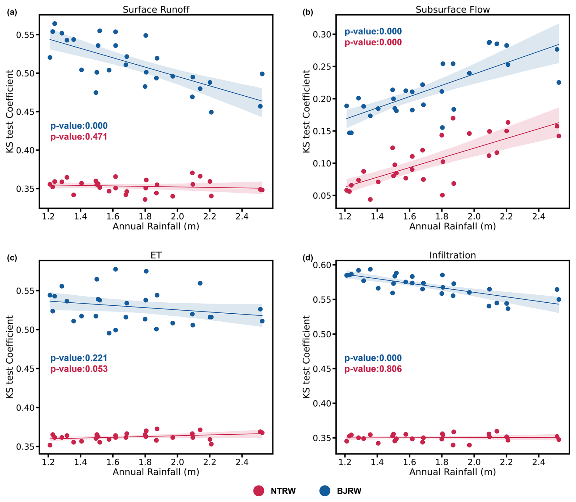
Figure 13 Scatter plots of KS test coefficients between LULCC and four model outputs under 29 years of different annual rainfall amounts, with statistical significance levels indicated by the p values in the plots. Shaded areas indicate 95 % confidence intervals. Regression equations for surface runoff at (a) the NTRW ($y=\mathrm{0.36}-\mathrm{0.003}x$) and BJRW ($y=\mathrm{0.62}-\mathrm{0.06}x$). Subsurface flow at (b) the NTRW ($y=-\mathrm{0.03}+\mathrm{0.08}x$) and BJRW ($y=\mathrm{0.06}+\mathrm{0.09}x$). ET at (c) the NTRW ($y=\mathrm{0.35}+\mathrm{0.01}x$) and BJRW ($y=\mathrm{0.55}-\mathrm{0.01}x$). Infiltration at (d) the NTRW ($y=\mathrm{0.35}+\mathrm{0.001}x$) and BJRW ($y=\mathrm{0.63}-\mathrm{0.03}x$).

4.4.2 Rainfall intensifies the changes in groundwater caused by LULCC

Figure 10 presents scatter plots correlating KS test values for four hydrological outputs with 29 years of annual rainfall data, evaluating how the impacts of LULCC vary under different precipitation intensities. Our analysis highlights significant variability in the effects of LULCC across various annual rainfall amounts in the BJRW. Here, surface runoff and infiltration exhibit reduced variations before and after urbanization as annual rainfall increases, whereas variations in subsurface flow exhibit greater magnitude with increasing annual rainfall. In the NTRW, the most obvious changes are observed in annual subsurface flow, which also shows increased variation with higher levels of annual precipitation. In scenarios where all surfaces are permeable, an increase in annual rainfall leads to progressive soil saturation, consequently enhancing surface runoff and reducing water infiltration. This pattern is similar to that observed on impervious surfaces. As annual rainfall increases, the disparities in surface runoff and infiltration between different land use patterns diminish. However, the impact on subsurface flow differs between permeable and impervious surfaces. In areas with high permeability, increased rainfall promotes soil saturation, enhancing subsurface flow. However, in areas dominated by impervious surfaces, limited infiltration capacity restricts groundwater recharge, resulting in poorly saturated zone connectivity and reduced subsurface flow. These contrasting responses lead to more substantial differences in subsurface flow patterns between different land use types as annual rainfall increases.

4.5 Further discussion

4.5.1 Patterns of surface and subsurface hydrological behavior

Surface and subsurface hydrological processes exhibit distinct differences in their temporal responses and controlling factors. Surface runoff and infiltration respond rapidly and intensely to rainfall events, primarily driven by precipitation at daily timescales, making it difficult to identify stable topographic controls. However, when extending to annual timescales, these quick-response processes gradually reveal their sensitivity to slope and elevation patterns. In contrast, subsurface hydrological processes show weaker direct responses to rainfall, instead relying more heavily on topographic features and upstream water contributions to determine flow patterns.

This research further demonstrates that integrated indicators like the TWI exhibit more pronounced predictive significance for soil moisture patterns at longer (annual) timescales (Seibert et al., 2003; Rinderer et al., 2014; Kopecký et al., 2021). At this temporal scale, soil moisture and groundwater distributions reach a relatively stable state, making topographic influences on both surface and subsurface hydrological processes more evident.

Additionally, urbanization-induced expansion of impervious surfaces has significantly altered surface hydrological processes, with impacts varying across regions and topographic conditions. In contrast to surface processes, urbanization's effects on subsurface flow are less pronounced (Fig. 11), with the most significant changes occurring in low-elevation regions (Fig. 10c), consistent with the findings of Siddik et al. (2022).

4.5.2 Suggestions for urban water resource management

Urban hydrology is a highly complex issue (McGrane, 2016; Qi et al., 2021). This research indicates that urban hydrological processes are influenced not only by local topography but also by the characteristics of the entire watershed. The effects of urbanization are not uniform but rather distinctly localized, with varying intensities across different spatial areas.

Cities located in steep and rainy watersheds, like Hong Kong SAR, face more severe challenges. Due to its steep mountainous terrain and limited flat regions, Hong Kong SAR has minimal zones suitable for stable water storage (Chen, 2001). Additionally, with its subtropical monsoon climate bringing intense rainfall during typhoon seasons, Hong Kong SAR faces significant urban flooding risks in its low-elevation, high-density building regions (He et al., 2021; Yang et al., 2022). Although flat cities like Shenzhen have the capability of buffering the effects of urbanization through flatter topography, their high level of urbanization still poses significant challenges for flood management under extreme-precipitation conditions. Constrained by space limitations, development has extended into floodplains, wetlands, and reclaimed coastal zones (Chan et al., 2014).

Evidence suggests that depending exclusively on hard-engineering infrastructure for urban flood defense is both costly and impractical (Chan et al., 2022; Cai et al., 2021). The role of non-structural flood control measures should be emphasized, including public participation and training, the development of comprehensive water resource monitoring networks, and hydrological models for more precise flood monitoring and prediction. Technology-driven warning systems have demonstrated their effectiveness in predicting urban flood risks (Yereseme et al., 2022). The experience of sustainable flood risk management in the UK, the Netherlands, the USA, and Japan provides useful lessons for developed cities worldwide (Chan et al., 2022). The use of hydrological modeling to combine flood risk assessment with urban planning leads to more resilient urban water management systems. In particular, the application of ISSHMs can greatly enhance predictive capabilities before implementing land use changes. By calibrating models to reflect current watershed conditions, planners can readily simulate various “what-if” scenarios to evaluate how proposed urban development patterns might alter hydrological processes.

4.5.3 Limitations and future work

Our study provides valuable insights into the effects of topography and LULCC on hydrological processes across various spatiotemporal scales in different watersheds. Although the hydrological model used was comprehensively calibrated using observational data and demonstrated accurate predictive capabilities, several limitations warrant consideration. Firstly, the calibration of the model parameters was conducted manually using local data, which may not encompass the optimal parameter sets unidentified in this study. Furthermore, the inherent uncertainties associated with the monitoring data and the model structure were not thoroughly evaluated. Due to the complexity of ISSHMs and the significant amount of time required to thoroughly assess all uncertainties, such evaluations remain challenging but are necessary for advancing the field. Secondly, our study area is located in a subtropical humid region characterized by frequent rainfall and consistently moist soils. This geographical specificity may limit the generalizability of our findings to regions with the same climatic conditions. Moreover, the rainfall data utilized in this study only encompassed the typical range of precipitation for the region; extreme-rainfall events, which may induce unique hydrological responses, were not investigated. The impact of such extreme conditions remains to be explored in future studies. Finally, the ET process differs from the other three processes as it is influenced not only by land cover but also by climatic factors, such as solar radiation, temperature, and humidity (Blyth, 1999). Our findings indicate that establishing a clear, general relationship between topography and ET is difficult. However, the analysis of LULCC and ET shows that converting forested areas into built-up land reduces the total ET at the watershed scale (Fig. 11). Since our research primarily focuses on terrestrial hydrological processes, the discussion of ET remains relatively limited.

5 Conclusions

Utilizing the ISSHM model, SHUD, this study explored the effects of topographical slope and urbanization-induced LULCC on surface runoff, subsurface flow, ET, and infiltration across various spatiotemporal conditions in two neighboring subtropical watersheds. Our findings reveal that both local topography (specifically local slope) and overall watershed topography significantly influence hydrological processes across different temporal and spatial scales. At the daily scale, precipitation emerges as the dominant control factor for rapid hydrological processes (infiltration and surface runoff), with local slope having limited influence. However, for slower processes like subsurface flow, local slope demonstrates a notable impact. At the annual scale, local slope correlates with both fast and slow hydrological processes in high-elevation areas. In low-elevation regions, the relationship between local slope and hydrological processes is more complex: flat watersheds show clear correlations between local slope and hydrological processes, while in steep watersheds, low-elevation hydrological processes might be more influenced by upstream contributions rather than local terrain slope.

The varying influences of local and overall watershed topography lead to spatially differentiated impacts of LULCC. Urbanization significantly increases surface runoff, while decreasing infiltration and ET, with a minimal impact on subsurface flow. Per unit of urbanized area, watersheds with gentler slopes demonstrate a greater capacity to mitigate LULCC effects, particularly in reducing the magnitude of increased surface runoff. However, this buffering capacity diminishes as annual precipitation increases. Additionally, the difference in subsurface flow between pre- and post-urbanization conditions becomes more pronounced with increased annual precipitation. This study underscores the importance of incorporating non-structural approaches in urban water management. Well-calibrated ISSHM models have demonstrated their practical value in land use scenario design, enabling rapid simulation of how different development patterns affect hydrological processes across temporal and spatial scales. The integration of such hydrological modeling with urban planning will help build more resilient cities.

Appendix A: SHUD hydrological process formulas

A comprehensive exposition of the governing equations for SHUD is provided in Shu et al. (2020). Here, the emphasis is placed on expounding the equations that are relevant to the processes addressed in this study.

• Infiltration. SHUD adopts the Richards equation like most ISSHMs, which is used to describe the infiltration process. While there are no general analytical solutions to the Richards equation, SHUD adopted the Green–Ampt infiltration equation (Eq. A1), which allows a simple form of Darcy's law to be used to calculate the infiltration rate q_i [L T⁻¹],

  $$\begin{array}{}\text{(A1)}& q_{\mathrm{i}}=K_{\mathrm{i}}\left(\mathrm{1}+{\displaystyle \frac{h_{\mathrm{s}}}{D_{\text{inf}}}}\right),\end{array}$$

  where h_s [L T⁻¹] is the ponding water height plus precipitation; D_inf [L] is the infiltration depth representing the top soil layer; and K_i [L T⁻¹] is the effective infiltration conductivity and a function of the soil saturation ratio, soil properties, and h_s. The Green–Ampt method assumes that the infiltrating wetting front forms a sharp jump from a constant initial moisture content ahead of the front to saturation at the front.

• Evapotranspiration. Potential evapotranspiration (PET) is computed using the Penman–Monteith equation (Eq. A2), while actual evapotranspiration (AET) is derived by multiplying PET by a soil moisture stress coefficient, determined by the soil moisture content and groundwater table depth.

  $$\begin{array}{}\text{(A2)}& \mathit{\lambda }E={\displaystyle \frac{{\mathrm{\Delta }}_{\mathrm{e}}H+{\mathit{\rho }}_{\mathrm{a}}{c}_p\left(e_{\mathrm{s}}\right(T_{\mathrm{z}})-e_{\mathrm{z}})/r_{\mathrm{a}}}{{\mathrm{\Delta }}_{\mathrm{e}}+\mathit{\gamma }(\mathrm{1}+r_{\mathrm{c}}/r_{\mathrm{a}})}}\end{array}$$

  Here, λ (= 2.4710⁶, J kg⁻¹) is the latent heat of evaporation, E [L T⁻¹] is the PET rate, Δ_e is the slope of the saturation vapor pressure versus temperature curve, H is the total available energy, ρ_a is the density of the air, c_p is the specific heat capacity of the air, e_s(T_z) is the saturated vapor pressure at the height of z, e_z is the vapor pressure at the height of z, r_a and r_c are the two resistance coefficients, and γ is the psychrometric constant.

• Surface runoff. The kinematic-wave equation (Eq. A3) is used to approximate the surface runoff in the SHUD,

  $$\begin{array}{}\text{(A3)}& {\displaystyle \frac{\partial h}{\partial t}}=-{\displaystyle \frac{\partial \left(vh\right)}{\partial x}}-{\displaystyle \frac{\partial \left(vh\right)}{\partial y}}+r,\end{array}$$

  where h [L] represents the average depth of flow; v [L T⁻¹] is the flow velocity; and r [L T⁻¹] is the rate of addition or loss of water caused by precipitation, infiltration, and evaporation. The relationship between v and h is represented by the Manning equation (Eq. A4),

  $$\begin{array}{}\text{(A4)}& v=-{\displaystyle \frac{S_{\mathrm{0}}^{\frac{\mathrm{1}}{\mathrm{2}}}{h}^{\frac{\mathrm{3}}{\mathrm{5}}}}{n}},\end{array}$$

  where S₀ [–] is the surface slope, and n [$\mathrm{T}{\mathrm{L}}^{-\mathrm{1}/\mathrm{3}}$] is the Manning roughness.

• Subsurface flows. The SHUD applies the Richards equation (Eq. A5) to describe both saturated and unsaturated flows, and the water density is assumed to be constant,

  $$\begin{array}{}\text{(A5)}& \begin{array}{rl}{\displaystyle \frac{\partial \mathit{\theta }}{\partial t}}=& {\displaystyle \frac{\partial }{\partial x}}\left[K_x\left(\mathit{\theta }\right){\displaystyle \frac{\partial \mathrm{\Phi }}{\partial x}}\right]+{\displaystyle \frac{\partial }{\partial y}}\left[K_y\left(\mathit{\theta }\right){\displaystyle \frac{\partial \mathrm{\Phi }}{\partial y}}\right]\\ & +{\displaystyle \frac{\partial }{\partial z}}\left[K_z\left(\mathit{\theta }\right){\displaystyle \frac{\partial \mathrm{\Phi }}{\partial z}}\right],\end{array}\end{array}$$

  where θ [–] is the volumetric moisture content; K_x(θ) [L T⁻¹], K_y(θ) [L T⁻¹], and K_z(θ) [L T⁻¹] indicate hydraulic conductivity depending on direction and treated as a function of θ; and Φ [L] is the total potential ($\mathrm{\Phi }=\mathit{\psi }+z$, where ψ [L] is the capillary potential, and z is the elevation above the datum). SHUD utilizes the Van Genuchten functions to solve the relationship for soil moisture content, capillary potential, and hydraulic conductivity.

Appendix B: Assessment equations

Spearman's rank correlation method evaluates the strength and monotonic nature of relationships between two variables without relying on assumptions regarding data distribution or residuals. The KS two-sample test compares two samples to determine if they are drawn from the same distribution, without assumptions about the underlying distribution. The KS statistic is the maximum absolute difference between the CDFs of the two data vectors.

For the daily-scale analysis, we focused on positive model outputs during rainy days (precipitation ≥ 0.1 mm d⁻¹). We employed matrix D for each zone (Zone 1 to Zone 3) to assess daily outputs related to slope angle for each grid (Eqs. B1 and B2). Model outputs for surface runoff and subsurface flow (m³ d⁻¹) represent net flow amounts per mesh grid. For daily analysis, these outputs were summed to total flow volumes (m³) and divided by grid area to obtain flow depths (m). Infiltration and ET outputs (m d⁻¹) were similarly summed to daily depths (m). These standardized depths were used to analyze impacts of slope and LULCC:

$$\begin{array}{}\text{(B1)}& {\displaystyle }& {\displaystyle }\mathbf{D}=\left[\begin{array}{c}{\mathbf{W}}_{\mathrm{1}}\\ \mathrm{⋮}\\ {\mathbf{W}}_N\end{array}\right],\text{(B2)}& {\displaystyle }& {\displaystyle }{\mathbf{W}}_n=\left[\begin{array}{ccc}{y}_{\mathrm{1}n}& p_{\mathrm{1}}& s_n\\ \mathrm{⋮}& \mathrm{⋮}& \mathrm{⋮}\\ y_{\text{in}}& p_{\mathrm{i}}& s_n\end{array}\right].\end{array}$$

In matrix D, each row W_n ($n=\mathrm{1},\mathrm{2},\mathrm{\dots },N$) corresponds to the model outputs associated with a specific hydrological process of the nth grid. Within W_n, each row represents a rainy day under consideration, with i denoting the total number of rainy days analyzed. Each row comprises three values: the daily model output y_kn ($k=\mathrm{1},\mathrm{2},\mathrm{\dots },i$), the corresponding rainfall amount p_k ($k=\mathrm{1},\mathrm{2},\mathrm{\dots },i$), and the grid's slope angle s_n. Consequently, the Spearman correlation coefficient was computed between the transpose vectors ${\mathit{y}}_{N\times i}^{\mathrm{T}}$ and ${\mathit{s}}_{N\times i}^{\mathrm{T}}$.

To analyze LULCC effects, vectors H_d (Eq. B3) and C_d (Eq. B4) were generated for each grid under HLU and CLU patterns, and the KS test value was computed between these two vectors for each grid,

$$\begin{array}{}\text{(B3)}& {\displaystyle }& {\displaystyle }{\mathit{H}}_{\mathrm{d}}=[y_{\mathrm{1}\mathrm{|}\text{HLU}},y_{\mathrm{2}\mathrm{|}\text{HLU}},\mathrm{\dots },y_{i\mathrm{|}\text{HLU}}],\text{(B4)}& {\displaystyle }& {\displaystyle }{\mathit{C}}_{\mathrm{d}}=[y_{\mathrm{1}\mathrm{|}\text{CLU}},y_{\mathrm{2}\mathrm{|}\text{CLU}},\mathrm{\dots },y_{i\mathrm{|}\text{CLU}}],\end{array}$$

where i denotes the total number of rainy days, and y_k|HLU and y_k|CLU ($k=\mathrm{1},\mathrm{2},\mathrm{\dots },i$) represent the model daily output of this grid under the HLU pattern and the CLU pattern on the kth rainy day, respectively. We also calculated the absolute difference in mean values of these two vectors to quantify the magnitude of change between the two land use patterns in terms of their effects on the model outputs.

To evaluate the effects of slope on an annual scale, a new matrix A is constructed as follows (Eq. B5):

$$\begin{array}{}\text{(B5)}& \mathbf{A}=\left[\begin{array}{cc}{y}_{\mathrm{1}}& s_{\mathrm{1}}\\ \mathrm{⋮}& \mathrm{⋮}\\ y_N& s_N\end{array}\right],\end{array}$$

where N represents the number of grids within each zone, and y_n and s_n ($n=\mathrm{1},\mathrm{2},\mathrm{\dots },N$) denote the annual output and slope angle for the nth grid, respectively. Only grids with annual volumes exceeding 10 mm were considered for surface runoff and subsurface flow analysis to concentrate on pronounced flows. Subsequently, the Spearman correlation coefficient was calculated between the transpose vectors ${\mathit{y}}_N^{\mathrm{T}}$ and ${\mathit{s}}_N^{\mathrm{T}}$.

The KS test was also applied at the annual scale to compare model outputs between HLU and CLU patterns across the entire subbasin range. Vectors H_y (Eq. B6) and C_y (Eq. B7) represent the annual model outputs under the HLU pattern and the CLU pattern, respectively.

$$\begin{array}{}\text{(B6)}& {\displaystyle }{\mathit{H}}_y=[y_{\mathrm{1}\mathrm{|}\text{HLU}},y_{\mathrm{2}\mathrm{|}\text{HLU}},\mathrm{\dots },y_{z\mathrm{|}\text{HLU}}]\text{(B7)}& {\displaystyle }{\mathit{C}}_y=[y_{\mathrm{1}\mathrm{|}\text{CLU}},y_{\mathrm{2}\mathrm{|}\text{CLU}},\mathrm{\dots },y_{z\mathrm{|}\text{CLU}}]\end{array}$$

Here, z denotes the number of grids across each subbasin, and y_k|HLU and y_k|CLU ($k=\mathrm{1},\mathrm{2},\mathrm{\dots },z$) represent the model annual output of the kth grid under the HLU pattern and the CLU pattern, respectively. The KS test was then carried out between these two vectors.

Appendix C: Supplementary calibration results

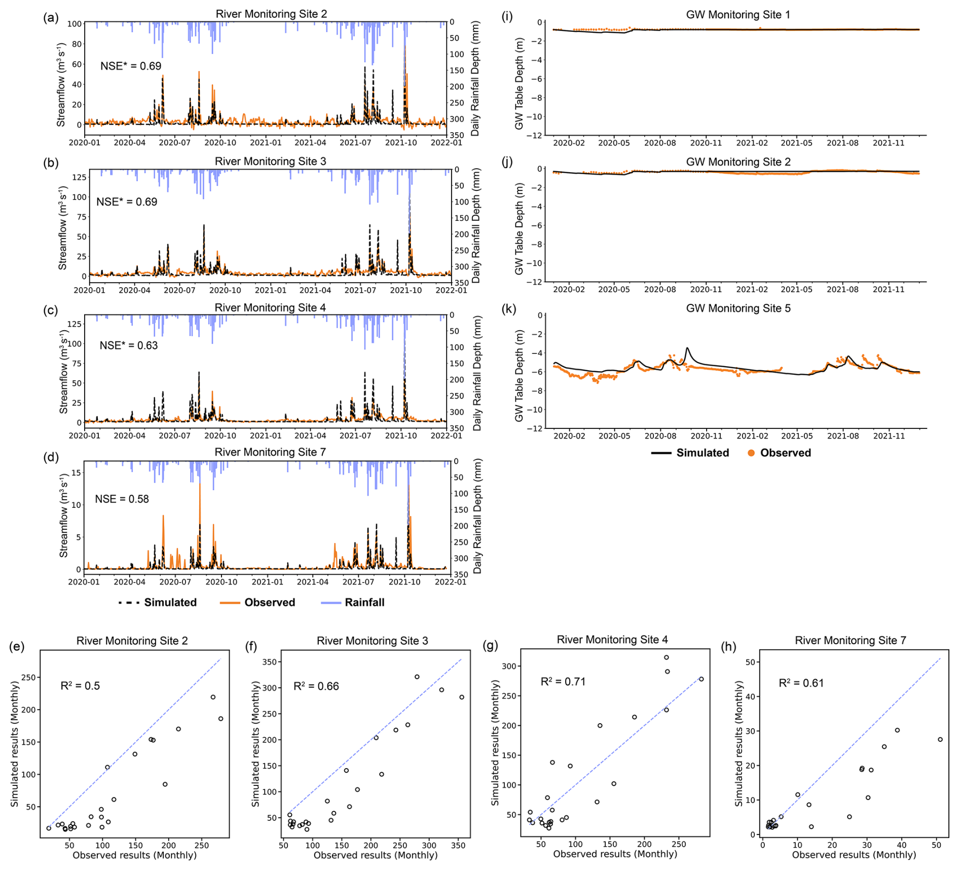
Figure C1 Other sites' calibration results across daily river discharge (a)–(d) and monthly river discharge (e)–(h), as well as groundwater table depth (i)–(k).