From hydraulic root architecture models to efficient macroscopic sink terms including perirhizal resistance: quantifying accuracy and computational speed

Root water uptake strongly affects soil water balance and plant development. It can be described by mechanistic models of soil–root hydraulics based on soil water content, soil and root hydraulic properties, and the dynamic development of the root architecture. Recently, novel upscaling methods have emerged, which enable the application of detailed mechanistic models on a larger scale, particularly for land surface and crop models, by using mathematical upscaling.

In this study, we explore the underlying assumptions and the mathematical fundamentals of different upscaling approaches. Our analysis rigorously investigates the errors introduced in each step during the transition from fine-scale mechanistic models, which considers the nonlinear perirhizal resistance around each root, to more macroscopic representations. Upscaling steps simplify the representation of the root architecture, the perirhizal geometry, and the soil spatial dimension and thus introduces errors compared to the full complex 3D simulations. In order to investigate the extent of these errors, we perform simulation case studies, spring barley as a representative non-row crop and maize as a representative row crop, using three different soils.

We show that the error introduced by the upscaling steps strongly differs, depending on root architecture and soil type. Furthermore, we identify the individual steps and assumptions that lead to the most important losses in accuracy. An analysis of the trade-off between model complexity and accuracy provides valuable guidance for selecting the most suitable approach for specific applications.

1 Introduction

Plant transpiration plays a vital role in the overall soil water balance and is a sensitive process in land surface and crop models, accounting for 61 %–75 % of the total evapotranspiration (Schlesinger and Jasechko, 2014) and 10 %–15 % of the total global evaporation (Ruhoff et al., 2022). A mechanistic description of how plant transpiration is influenced by soil and root properties helps to unravel the interaction between climate, soil water balance, and plant development. Such models can support plant breeding efforts to find root traits aiming for more drought-resistant plants in specific pedoclimatic environments and empower decision-makers in optimizing agricultural practices for improved crop water management and sustainable land use (Louarn and Song, 2020; Soualiou et al., 2021).

The soil–plant system is a multi-scale hierarchically structured system with typical structures that exist and influence or control processes at different scales. At the smallest scale, water flow in soils depends on the structure of the water-filled pore network, i.e. the size of water-filled pores and water films on solid surfaces and their connectivity. In plants, this scale corresponds to the water flow in cell walls through cell membranes and through water-conducting vessels, i.e. xylem vessels. The arrangement of cells in tissues, the constitution of cell walls, and the size of xylem vessels and the pits in their sieve plates control water flow in root system. Using models that solve Navier–Stokes equations, hydraulic properties that define the averaged flow over these smaller-scale structures as a function of averaged water potential gradients can be derived. For porous media, Darcy's law can be derived from the Navier–Stokes equations using homogenization (Hornung, 1996). Also, in plants, water flow is generally laminar. Couvreur et al. (2018) describe water movement within root cross-sections, numerically calculating effective radial conductivity from root anatomical features. The effective hydraulic properties can subsequently be used to describe the averaged flow as a function of averaged water potential using continuum equations.

In summary, Darcy-type flow equations are used to simulate water flow in both the soil and the root domains and in the water exchange between them. However, the small diameter of roots ($\approx \mathrm{1}\times {\mathrm{10}}^{-\mathrm{4}}$ m) with respect to their length (≈1 m) leads to very small diameter-to-length ratios $O(\mathrm{1}\times {\mathrm{10}}^{-\mathrm{4}})$. The size of the root zone requires very small discretizations with respect to the size of the simulation domain to accurately represent the fluxes and water potential. Therefore, a so-called 1D–3D mixed-model approach is used (Koch et al., 2018), where the flow in the soil is described using a 3D continuum equation, i.e. the Richards equation. This approach will be the starting point of our upscaling.

The flow in the root system is represented by a network of porous pipes with pipe walls representing the root tissues through which water flows radially towards the xylem tissue that represents the internal part of the tube where water flows axially. The flow in each xylem segment is described as a function of the water potential gradient along the xylem and the exchange between the root and the soil as a function of the water potential difference between the soil–root interface and the water in the root xylem tissue. The root system is assumed not to occupy a volume in the soil domain, and the water flow between the soil and root domains is represented by a source/sink term in the soil domain. The information that needs to be exchanged between the two domains is the water potential and water fluxes at the soil–root interface.

Schnepf et al. (2023, 2020) recently benchmarked such functional-structural root architecture models for simulating the root water uptake (RWU) from drying soils. A central part is the coupling between the two domains. In the 3D soil model, the water potential is calculated at the nodes or the centres of the grid cells that are used to discretize the 3D soil domain. The 3D soil model, in which RWU is represented as a source or sink term, does not resolve the fluxes and water potential gradients around the root segments within a grid cell. In order to obtain water potential at the soil–root interface, which is used by the root model, a perirhizal model around the root segments is employed that incorporates nonlinear soil conductance based on Schröder et al. (2008). This is crucial, since Khare et al. (2022) showed that, in drying soils, a mere increase in grid resolution fails to accurately characterize the sharp gradients in soil water potential. Following Vanderborght et al. (2023) the perirhizal zone is approximated by a cylindrical domain. Typically, the domain volume is approximated in proportion to the segment's root length, surface, or volume in a given macroscopic soil element volume (e.g. De Bauw et al., 2020; Mai et al., 2019). It is well known that the inter-root distance influences the uptake potential (de Willigen, 1987) due to inter-root competition, and Graefe et al. (2019) underline the importance of the outer perirhizal cylinder radii distribution. Kohl et al. (2007) used Voronoi diagrams to determine the outer radii in 2D, where the Voronoi faces are located exactly at mid-distance between the roots and therefore separate the corresponding perirhizal zones. Schlüter et al. (2018) used distance functions in 3D to quantify the perirhizal zone. In this work, we present a novel approach using Voronoi diagrams in 3D, where the Voronoi cells describe the perirhizal volumes.

Moving to larger-scale models, the first obvious step is to reduce the dimensions of the macroscopic soil model. RWU was simulated by de Willigen et al. (2012) at different complexities, using 1D, 2D, and 3D soils. They found that acknowledging the lateral water potential gradients resulted in a reduction in simulated actual transpiration. However, they considered a soil with the same lateral (x and y) dimension, with the root system in the middle, which is not consistent with the inter-plant and inter-row distances of most agricultural crops. Couvreur et al. (2014) demonstrated that failing to account for lateral variations in root density and bulk soil water potential results in an overestimation of simulated collar water potential for row crops but works sufficiently well for crops with rather uniform lateral root distributions.

The representation of the root architecture in an upscaled, e.g. 1D, soil water flow model can be of different complexity. When the 3D root architecture model is coupled with a 1D soil model, a first assumption is that the water potential at the soil–root interface is uniform at a given depth or in a certain layer of the discretized 1D soil profile. Therefore, we use a representation of a mean behaviour, where the variance is captured only when using higher-dimensional models. When the hydraulic root system model is assumed to be linear, i.e. it is assumed that the conductance of the different segments does not depend on the water potential, then an exact upscaled root hydraulic model can be derived (Vanderborght et al., 2021). This exact upscaled model can be approximated by a so-called parallel root model that assumes that the water that is taken up by root segments in a certain soil layer is directly transferred to the root collar through an effective, laterally impermeable root pipe that does not exchange water with other soil layers so that RWU from different soil layers occurs in parallel (Couvreur et al., 2014; Vanderborght et al., 2021). Vanderborght et al. (2021) demonstrated that this approach well reproduced the water uptake by 3D root architectures. When the root architecture model is coupled with a 1D soil model, the 1D soil model simulates the bulk soil water potential and assumes that they are uniform at a certain depth. When the soil is sufficiently wet and the hydraulic conductivity of the soil is sufficiently large, the soil water potential at the soil–root interface can be assumed to be equal to the bulk soil water potential. However, when soils dry out, the water potential at the soil–root interface differs from the bulk soil water potential and depends on the flow to a specific root segment. In order to couple the 3D root architecture model with an upscaled 1D soil model, Vanderborght et al. (2023) used cylindrical perirhizal models around the single-root segments and assumed that the bulk soil water potential and outer radii of the perirhizal cylinders were the same for all root segments. The perirhizal radii were derived assuming that all roots in a soil layer were parallel and equidistant, which is a good approximation when roots are homogeneously distributed. To simplify the model further, they used a parallel root model assuming that the xylem water potential in and the water flow to each root segment in a certain soil layer were the same. Despite the fact that the flow rate and water potential in the xylem and at the soil–root interface of root segments of the 3D architecture that was coupled to the 1D model varied a lot between the root segments, the parallel root model described both the total RWU from a soil layer and the overall transpiration quite well and with strongly reduced computational costs.

However, the consequences of assuming uniform bulk soil water potential were not considered in Vanderborght et al. (2023, 2021). In this study, we systematically test these new upscaling methods for the first time for scenarios that represent the distribution of plants in an agricultural field. We use spring barley as a representative non-row crop and maize as a representative row crop. We simulate plant transpiration over 2 weeks in three soil types (loam, clay, and sandy loam) to observe soil water depletion and the occurrence of plant water stress. We perform the simulations with the full hydraulic 3D model and compare the accuracy of the approximations in each upscaling step.

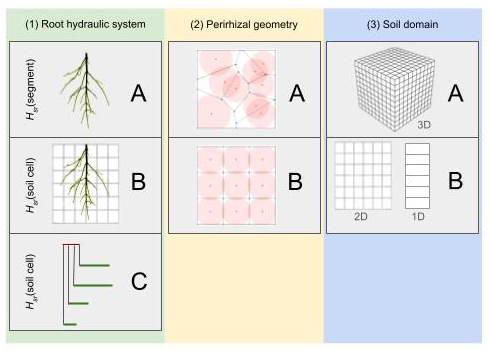
Figure 1 The green column shows the simplification of RWU regarding the root architecture: (A) full model, (B) exactly upscaled with uniform soil–root interface water potential per soil cell, (C) parallel root model. The yellow column shows a 2D representation of the perirhizal radii computation using (A) Voronoi diagrams or (B) uniform perirhizal radii in a soil element. The blue column describes the dimensionality of the macroscopic soil domain: (A) full 3D or (B) cases where we assume that the soil water potential does not change in specific directions.

The full root hydraulic architecture model combined with a 3D soil model enables us to analyse spatial water depletion in detail. However, the computational costs make it inefficient for large-scale applications. Also, the full hydraulic root architecture is not easily included in large-scale models, and it is preferable to use an RWU sink term that is only based on the soil states explicitly. Vanderborght et al. (2023) showed how such sink terms can be derived from more mechanistic models using 3D root hydraulics. We divide the different upscaling steps into three categories (see Fig. 1) and analyse the steps regarding accuracy and speed:

1. The way the root hydraulic system is represented (green column). The surrounding soil of the root system is characterized by soil water potential at the soil–root interface for each root segment (Fig. 1, A(1)) or is given for each soil element of the macroscopic soil grid (Fig. 1, B(1)). The third choice is to approximate the root architecture by a parallel root system with similar macroscopic hydraulic properties (Fig. 1, C(1)).

2. The way the radius of the perirhizal zone is calculated (yellow column). The first option uses 3D Voronoi diagrams to obtain the volume of the perirhizal zone (Fig. 1, A(2)), or homogeneously distributed roots are assumed within each soil cell (Fig. 1, B(2)).

3. The dimensionality of the soil model (blue column). Either the macroscopic soil is described in full 3D (see Fig. 1, A(3)) or the soil is approximated by a lower-dimensional model, where we assume the soil water potential does not change in specific directions (see Fig. 1, B(3)).

We use the three columns of Fig. 1 for a precise categorization of the upscaling steps involved, choosing a triple where the first letter denotes the root hydraulic system, the second denotes the way the perirhizal zone is calculated, and the third denotes the dimensionality of the model. In this way, AAA := A(1)A(2)A(3) describes the most accurate model, and CBB := C(1)B(2)C(3) describes the fastest and coarsest model, and we use a lower-case “x” to indicate the choice of any model; e.g. Axx is all possible models where the full 3D root hydraulic model is calculated; therefore soil water potential at the soil–root interface is given for each root segment.

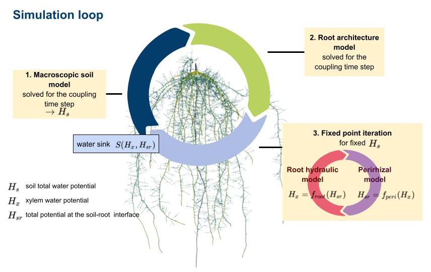
Figure 2 The main simulation loop first solves the macroscopic soil model yielding the total soil potential H_s; next, optionally, root architectural development; and, finally, finds consistent values for the total xylem water potential H_x and soil–root interface potential H_sr using a fixed-point iteration. Sink terms are calculated from the potentials H_x and H_sr.

2 Materials and methods

We describe water flow in the plant–rhizosphere–soil system by regarding each subdomain as mathematical sub-problems that are solved sequentially (see Koch et al., 2021, for alternative monolithic schemes). We sequentially compute the macroscopic soil model (Sect. 2.1) and the root architecture development (Sect. 2.2) and use a fixed-point iteration, where we solve the root hydraulic model and the perirhizal model (Sect. 2.3). From the resulting root xylem potentials H_x and the total potentials at the root–soil interface H_sr, the RWU is determined, which then acts as a sink for the macroscopic soil model; see Fig. 2. Table 1 presents a summary of all variables and parameters of the models.

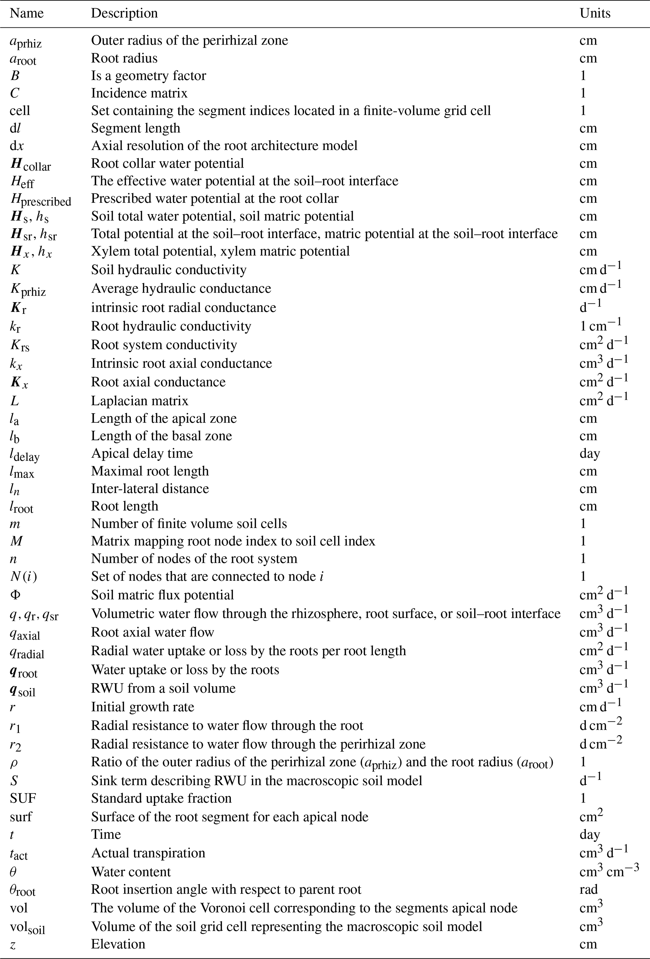
Table 1 Overview of parameter and variable names in alphabetical order.

The models were implemented in CPlantBox (Zhou et al., 2020; Schnepf et al., 2018) and dumux-rosi (Giraud et al., 2023), which are available on GitHub and are open-source, which facilitates reproducibility and further advancements (Barba, 2022). The use of upscaled models fundamentally increases performance. Depending on the root architecture and soil type, we could achieve speed-ups up to 15000 %. We discuss the trade-off between model accuracy and computational speed which guides users how to pick the appropriate modelling approach for specific applications.

In the following, we describe each part of Fig. 2 in detail: firstly the macroscopic soil model (Sect. 2.1), the root architecture development model (Sect. 2.2), and the fixpoint iteration, where we iterate the full root hydraulic model and the perirhizal model (Sect. 2.3). These models are of type Axx (see Fig. 1). We present two upscaled models: the upscaled aggregated model (Sect. 2.5), corresponding to the models Bxx, and the parallel root model (Sect. 2.6), corresponding to the models Cxx. Next, we describe the two approaches to obtain the outer perirhizal radii (Sect. 2.4) corresponding to the models xAx and xBx. Finally, in Sect. 2.7, we define test scenarios to benchmark the efficiency of the simplifications of the larger-scale models against the reference full hydraulic model.

2.1 Macroscopic soil model

Water movement is described by the Richards equation,

$$\begin{array}{}\text{(1)}& {\displaystyle \frac{\partial \mathit{\theta }}{\partial t}}=\mathrm{\nabla }\cdot \left(K\left(\mathit{\theta }\right)\mathrm{\nabla }{\mathit{H}}_{\mathrm{s}}\right)+S,\end{array}$$

where θ (cm³ cm⁻³) is the water content, K (cm d⁻¹) is the soil hydraulic conductivity, H_s (cm) is the total soil water potential, and S is a sink term that describes RWU (d⁻¹).

We can solve the Richards equation in 3D (these models are named xxA) or assume no change in water potential in specific directions using a 1D or 2D soil grid (xxB). We use the finite volume solver DuMu^x (Koch et al., 2021) to numerically solve Eq. (1). The sink, our source S, is calculated for each finite volume cell as a function of the root xylem total potentials H_x and the total potentials at the root surface interface H_sr. Generally, H_sr is derived as a function of H_x and H_s using a perirhizal model, as described in Sect. 2.3. For each finite volume cell i, the sink or source S_i (cm³ d⁻¹) is calculated as

$$\begin{array}{}\text{(2)}& S_i=\sum _{j\in {\text{cell}}_i}\mathrm{2}{a}_{\mathrm{root},j}\mathit{\pi }{k}_{\mathrm{r},j}\mathrm{d}{l}_j(H_{\mathrm{sr},j}-H_{x,j}),\end{array}$$

where j is the root segment index of a segment located within the finite volume cell i, a_root,j (cm) is the root radius, k_r,j (d⁻¹) is the intrinsic root radial conductivity, dl_j (cm) is the segment length, H_sr,j (cm) is the total potential at the soil–root interface, and H_x,j (cm) is the segment xylem total potential.

The relation between θ and the soil matric potential h_s is given by the water retention curve, which we describe using the Van Genuchten model (Van Genuchten, 1980). The conversion between total and matric potentials can readily take place as

$$\begin{array}{}\text{(3)}& h_{\mathrm{s}}=H_{\mathrm{s}}-z,\end{array}$$

where z is the elevation.

2.2 Root architecture development model

We use the model CPlantBox to describe the root architecture (Giraud et al., 2023; Zhou et al., 2020; Schnepf et al., 2018), which is able to represent the development of different root architecture geometries. CPlantBox is an open-source software, and the code is available at https://github.com/Plant-Root-Soil-Interactions-Modelling/CPlantBox (last access: 30 December 2024). The root architecture is represented as straight 1D segments in 3D space (1D/3D), where the segment length is less than or equal to the axial resolution dx.

Parameters are defined per root type and given by a mean and standard deviation to mimic the stochastic nature of the root system. Typical parameters are the insertion angle (θ_root), the length of the basal zone (l_b), the inter-lateral distance (l_n), the maximal root length (the number of laterals is deduced from maximal length) (l_max), the length of the apical zone (l_a) or apical delay time (l_delay), the root radius (a_root), and the initial growth rate (r), as well as type and probability of successor roots. We chose root architecture parameter sets for spring barley according to Eloundou (2021) based on Postma et al. (2017) and for maize according to Landl et al. (2018), which are available within the CPlantBox repository.

CPlantBox is a relatively generic code that allows different models of elongation rate, branching patterns, tropisms, and root senescence. In this study, we assumed negative exponential growth independently of any environmental influences such as soil temperature or bulk density. Likewise, branching patterns and insertion angles are not influenced by environmental conditions. Root radii are constant per root branch. The root types which can emerge from a given parent root are determined by root order. With these relatively simple root architecture simulations, we still produce realistic root system geometries that allow us to determine the effects of those geometries and, in particular, their heterogeneities on the upscaling results.

2.3 Root hydraulic and perirhizal model (Axx)

We use the model of Doussan et al. (1998) and in the following describe it using methods from graph theory. Along each root segment, the axial water flow is driven by the gradient of the total xylem water potential, and it is given by

$$\begin{array}{}\text{(4)}& q_{\mathrm{axial}}=k_x\mathrm{\nabla }{\mathit{H}}_x,\end{array}$$

where q_axial (cm³ d⁻¹) is the axial water flow, k_x (cm³ d⁻¹) is the intrinsic root axial conductance, and H_x (cm) is the total xylem water potential. The radial water flow is given for each root node i as

$$\begin{array}{}\text{(5)}& q_{\mathrm{radial},i}=\mathrm{2}\mathit{\pi }{a}_{\mathrm{root},i}{k}_{\mathrm{r},i}({\mathit{H}}_{\mathrm{sr},i}-{\mathit{H}}_{x,i}),\end{array}$$

where q_root,i (cm² d⁻¹) is the radial water flow per root length at node i, a_root,i (cm) is the root radius, k_r,i (d⁻¹) is the intrinsic root radial conductance, and H_sr,i (cm) is the total soil water potential at the soil–root interface. In agreement with Doussan et al. (1998), we consider that the soil water is a dilute solution, as is the sap; therefore we neglect the osmotic potential in the xylem and the soil.

The root system can be interpreted as a directed graph of n nodes and n−1 edges representing the root segments. The axial water flow (Eq. 4) is approximated by

$$\begin{array}{}\text{(6)}& q_{\mathrm{axial},i,j}\approx k_x{\displaystyle \frac{{\mathit{H}}_{x,j}-{\mathit{H}}_{x,i}}{\mathrm{d}{l}_{i,j}}},\end{array}$$

where (i,j) is the edge connecting node i and j and dl_i,j is the length of this segment (cm). In this context, Kirchhoff's law just states that the axial fluxes equal the radial flux at each node i. All volume fluxes going into the node must leave the node again; i.e. we assume that there is no water storage inside the root. Thus,

$$\begin{array}{}\text{(7)}& \sum _{j\in N\left(i\right)}{q}_{\mathrm{axial},i,j}=q_{\mathrm{radial},i},\end{array}$$

where i and j are node indices and N(i) shows the indices of the edges (i,j) in the graph. Note that, in the sum on the left-hand side, H_x,i occurs for each edge ij, which is the degree of node i, and H_x,j enters exactly once for each j∈N(i). Therefore, we can use the Laplace matrix L to easily describe Kirchhoff's law (Eq. 7) in matrix notation:

$$\begin{array}{}\text{(8)}& \mathbf{L}\left[\begin{array}{c}{\mathit{H}}_{\mathrm{collar}}\\ {\mathit{H}}_x\end{array}\right]=\left[\begin{array}{c}{t}_{\mathrm{act}}\\ {\mathit{q}}_{\mathrm{root}}\end{array}\right],\end{array}$$

where the symmetric Laplacian matrix $\mathbf{L}\in {\mathbb{R}}^{n\times n}$ is given by

$$\begin{array}{}\text{(9)}& \mathbf{L}=\mathbf{C}\text{diag}\left({\mathit{K}}_x\right){\mathbf{C}}^T\end{array}$$

and $\mathbf{C}\in {\mathbb{R}}^{n\times n-\mathrm{1}}$ is the graph's incidence matrix, where the ijth entry is equal to −1 when edge j is leaving node i and 1 when edge i arrives in node j. The matrix K_x is the $(n-\mathrm{1})\times \mathrm{1}$ vector of root axial conductances (cm² d⁻¹), where

$$\begin{array}{}\text{(10)}& ({\mathit{K}}_x{)}_i={\mathit{K}}_{x,i}=k_{x,i}/l_{\mathrm{root},i},\end{array}$$

with k_x,i being the intrinsic root axial conductance (cm³ d⁻¹) and l_root,i being the segment length (cm) of root segment with apical node index i. H_collar is the total root collar potential (cm), and H_x is the $(n-\mathrm{1})\times \mathrm{1}$ vector of the total root water potential (cm) of the other root nodes. On the right-hand side of Eq. (8), the value t_act describes the actual volumetric transpiration at the root collar (cm³ d⁻¹), and q_root (cm³ d⁻¹) describes the sources (positive sign) and sinks (negative sign) which represent water uptake from soil or water loss into soil by the roots. To solve specific root hydraulic scenarios, we need to define the RWU and adjust Eq. (8) to include root collar boundary conditions.

The volumetric RWU q_root (cm³ d⁻¹) is given for a total xylem potential H_x (cm) and a total water potential at the soil–root interface H_sr (cm) as

$$\begin{array}{}\text{(11)}& {\mathit{q}}_{\mathrm{root}}=\text{diag}\left({\mathit{K}}_{\mathrm{r}}\right)({\mathit{H}}_{\mathrm{sr}}-{\mathit{H}}_x),\end{array}$$

where H_sr is the $(n-\mathrm{1})\times \mathrm{1}$ vector of the total soil water potential at the soil–root interface and K_r is the $(n-\mathrm{1})\times \mathrm{1}$ vector of the root radial conductances (cm² d⁻¹), where

$$\begin{array}{}\text{(12)}& ({\mathit{K}}_{\mathrm{r}}{)}_i={\mathit{K}}_{\mathrm{r},i}=\mathrm{2}{a}_{\mathrm{root},i}\mathit{\pi }{l}_{\mathrm{root},i}{k}_{\mathrm{r},i},\end{array}$$

k_r,i being the intrinsic root radial conductance (d⁻¹) and a_root,i being the root segment radius (cm) of root segment i.

Including a Dirichlet boundary condition at the root collar, which is assumed to be located at the first node, Eq. (8) can be rewritten as

$$\begin{array}{}\text{(13)}& {\mathbf{L}}_{\mathrm{d}}\left[\begin{array}{c}{\mathit{H}}_{\mathrm{collar}}\\ {\mathit{H}}_x\end{array}\right]=\left[\begin{array}{c}{H}_{\mathrm{prescribed}}\\ \text{diag}\left({\mathit{K}}_{\mathrm{r}}\right)({\mathit{H}}_{\mathrm{sr}}-{\mathit{H}}_x)\end{array}\right],\end{array}$$

where L_d is the Laplacian matrix adjusted for the Dirichlet boundary condition such that the first entry of the first row is equal to 1 and all other entries are zeros. If we want to solve for H_x we can rewrite the above equation as

$$\begin{array}{}\text{(14)}& -{\mathit{K}}_{x,\mathrm{1}}{\mathit{e}}_{\mathrm{1}}{\mathit{H}}_{\mathrm{collar}}+{\mathbf{L}}_{n-\mathrm{1}}{\mathit{H}}_x=\text{diag}\left({\mathit{K}}_{\mathrm{r}}\right){\mathit{H}}_{\mathrm{sr}}-\text{diag}\left({\mathit{K}}_{\mathrm{r}}\right){\mathit{H}}_x,\end{array}$$

where L_n−1 is the $(n-\mathrm{1})\times (n-\mathrm{1})$ submatrix of L with removed first row and column and e₁ is the $(n-\mathrm{1})\times \mathrm{1}$ unit vector (see also Vanderborght et al., 2021, Eq. A5). Then, for any known H_sr, we can solve for H_x as

$$\begin{array}{}\text{(15)}& \underset{=:\mathbf{A}}{\underbrace{({\mathbf{L}}_{n-\mathrm{1}}+\text{diag}({\mathit{K}}_{\mathrm{r}}\left)\right)}}{\mathit{H}}_x=\underset{=:{\mathit{b}}_{\mathrm{d}}}{\underbrace{\text{diag}\left({\mathit{K}}_{\mathrm{r}}\right){\mathit{H}}_{\mathrm{sr}}+{\mathit{K}}_{x,\mathrm{1}}{\mathit{e}}_{\mathrm{1}}{\mathit{H}}_{\mathrm{collar}}}},\end{array}$$

where A is symmetric and diagonal dominant for (K_r)_i>0, and therefore positive definite and the right-hand side b depends on the matric potential of the soil–root interface H_sr and the total root collar potential H_collar.

When developing larger-scale soil models, we generally do not want to consider individual root water potential, since it is not feasible to explicitly describe the root architecture in such models. Thus, the effective sink term for RWU should be formulated in a way such that the values H_x are not explicitly needed. For Dirichlet boundary conditions, we calculate H_x from Eq. (15) and insert it into the Eq. (11) which describes RWU as

$$\begin{array}{}\text{(16)}& {\displaystyle }\begin{array}{rl}{\mathit{q}}_{\mathrm{root}}& =\text{diag}\left({\mathit{K}}_{\mathrm{r}}\right)({\mathit{H}}_{\mathrm{sr}}-({\mathbf{A}}^{-\mathrm{1}}\text{diag}\left({\mathit{K}}_{\mathrm{r}}\right){\mathit{H}}_{\mathrm{sr}}\\ & +{\mathbf{A}}^{-\mathrm{1}}{\mathit{K}}_{x,\mathrm{1}}{\mathit{e}}_{\mathrm{1}}{\mathit{H}}_{\mathrm{collar}}\left)\right),\end{array}\text{(17)}& {\displaystyle }\begin{array}{rl}{\mathit{q}}_{\mathrm{root}}& =\text{diag}\left({\mathit{K}}_{\mathrm{r}}\right)(\mathbf{I}-{\mathbf{A}}^{-\mathrm{1}}\text{diag}({\mathit{K}}_{\mathrm{r}}\left)\right){\mathit{H}}_{\mathrm{sr}}\\ & -\text{diag}\left({\mathit{K}}_{\mathrm{r}}\right){\mathbf{A}}^{-\mathrm{1}}{\mathit{K}}_{x,\mathrm{1}}{\mathit{e}}_{\mathrm{1}}{\mathit{H}}_{\mathrm{collar}},\end{array}\end{array}$$

corresponding to Vanderborght et al. (2021), Eq. (A16). For big, sparse matrices A, it is not efficient to compute A⁻¹, since this matrix is dense, so we express above equation as

$$\begin{array}{}\text{(18)}& \underset{=:{\mathbf{A}}_q}{\underbrace{\mathbf{A}\text{diag}({\mathit{K}}_{\mathrm{r}}{)}^{-\mathrm{1}}}}{\mathit{q}}_{\mathrm{root}}=\underset{=:{\mathit{b}}_q}{\underbrace{(\mathbf{A}-\text{diag}({\mathit{K}}_{\mathrm{r}}\left)\right){\mathit{H}}_{\mathrm{sr}}-{\mathit{K}}_{x,\mathrm{1}}{\mathit{e}}_{\mathrm{1}}{\mathit{H}}_{\mathrm{collar}}}}.\end{array}$$

and we can solve this sparse linear system for q_root for given H_sr and H_collar (note that diag(K_r)⁻¹ is sparse).

We can easily switch between Dirichlet boundary conditions, where we set the total potential H_collar (cm) at the root collar, and Neumann boundary conditions, where we predetermine a volumetric transpiration t_act (cm³ d⁻¹). In the simulation, the boundary condition will automatically be switched between Neumann and Dirichlet, ensuring that the root collar potential cannot be below a critical potential where we assume the plant's wilting point. The relationship between $t_{\mathrm{act}}={\sum }_i{\mathit{q}}_{\mathrm{root},i}$ and H_collar is given by

$$\begin{array}{}\text{(19)}& {\displaystyle }{t}_{\mathrm{act}}=K_{\mathrm{rs}}(H_{\mathrm{eff}}-{\mathit{H}}_{\mathrm{collar}}),\text{(20)}& {\displaystyle }{\mathit{H}}_{\mathrm{collar}}=(K_{\mathrm{rs}}{H}_{\mathrm{eff}}-t_{\mathrm{act}})/K_{\mathrm{rs}},\end{array}$$

where K_rs (cm² d⁻¹) is the root system conductivity, $H_{\mathrm{eff}}=\mathit{S}\mathit{U}{\mathit{F}}^T\cdot {\mathit{H}}_{\mathrm{sr}}$ (cm) is the effective water potential at the soil–root interface, and SUF (1) is the standard uptake fraction as defined by Couvreur et al. (2012), which corresponds with ${\mathit{q}}_{\mathrm{root}}/t_{\mathrm{act}}$ calculated for a uniform H_sr. Equation (19) is derived by summing up the rows of Eq. (17). For a detailed derivation we refer to Vanderborght et al. (2021), Appendix A.

In dry soils, RWU is often limited by low soil hydraulic conductivity near the root surface, i.e. in the perirhizal zone that is influenced by the radial water flow towards the root. Therefore, we consider an additional perirhizal resistance for each root segment as described by Vanderborght et al. (2023), which uses the approach of Schröder et al. (2008) to determine the total potential at the soil–root interface H_sr. We assume a steady rate in the cylindrical perirhizal zone, i.e. $\mathrm{d}\mathit{\theta }/\mathrm{d}t$ does not vary with radial distance from the root axis r. The steady-state model is not transient, and the model state only depends on the steady rate, which is determined from the bulk total soil water potential H_s and the root xylem potential H_x. Note that, with respect to the model application, the steady-rate approach can also be replaced by more complex dynamic rhizosphere models to determine H_sr (e.g. Khare et al., 2022; De Bauw et al., 2020; Mai et al., 2019).

The RWU of a single segment is given by

$$\begin{array}{}\text{(21)}& q_{\mathrm{r}}=\mathrm{2}{a}_{\mathrm{root}}\mathit{\pi }{l}_{\mathrm{root}}{k}_{\mathrm{r}}(H_{\mathrm{sr}}-H_x)={\displaystyle \frac{H_{\mathrm{sr}}-H_x}{r_{\mathrm{1}}}},\end{array}$$

where q_r (cm³ d⁻¹) is the volumetric flow rate (see Eqs. (11) and (12)) and $r_{\mathrm{1}}=(\mathrm{2}{a}_{\mathrm{root}}\mathit{\pi }{l}_{\mathrm{root}}{k}_{\mathrm{r}}{)}^{-\mathrm{1}}$ (d cm⁻²) is the radial resistance to water flow through the root.

The volumetric flow rate q_sr (cm³ d⁻¹) towards the soil–root interface through the perirhizal zone is equal to

$$\begin{array}{}\text{(22)}& q_{\mathrm{sr}}=\mathrm{2}\mathit{\pi }{l}_{\mathrm{root}}{K}_{\mathrm{prhiz}}B\left(H_{\mathrm{s}}-H_{\mathrm{sr}}\right)={\displaystyle \frac{H_{\mathrm{s}}-H_{\mathrm{sr}}}{r_{\mathrm{2}}}},\end{array}$$

where H_s (cm) is the mean total soil potential of the perirhizal zone of the segments and K_prhiz (cm d⁻¹) is the average hydraulic conductance in the perirhizal zone, defined by

$$\begin{array}{}\text{(23)}& K_{\mathrm{prhiz}}={\displaystyle \frac{\mathrm{\Phi }\left(h_{\mathrm{s}}\right)-\mathrm{\Phi }\left(h_{\mathrm{sr}}\right)}{H_{\mathrm{s}}-H_{\mathrm{sr}}}},\end{array}$$

where $\mathrm{\Phi }\left(h_c\right)={\int }_{-\mathrm{\infty }}^{h_c}K\left(h\right)\mathrm{d}h$ is the soil matric flux potential (cm² d⁻¹) and $h_{\mathrm{s}}:={\mathit{H}}_{\mathrm{s}}-z$ is the soil matric potential in the perirhizal cylinder corresponding to the average volumetric water content in that cylinder and to the soil matric potential of the macroscopic soil model. Furthermore, $h_{\mathrm{sr}}:={\mathit{H}}_{\mathrm{sr}}-z$ is the matric potential at the soil–root interface, B (1) is a geometry factor, and $r_{\mathrm{2}}=(\mathrm{2}{a}_{\mathrm{root}}\mathit{\pi }{l}_{\mathrm{root}}{K}_{\mathrm{prhiz}}B{)}^{-\mathrm{1}}$ (d cm⁻²) is the resistance to water flow through the perirhizal zone. The geometry factor B (1) is dependent on ρ (1), which is the ratio of the outer radius of the perirhizal zone a_prhiz (cm) and the root radius a_root (cm). The geometry factor is given by

$$\begin{array}{}\text{(24)}& {\displaystyle }B={\displaystyle \frac{\mathrm{2}({\mathit{\rho }}^{\mathrm{2}}-\mathrm{1})}{(\mathrm{1}-\mathrm{0.53}\mathit{\rho }{)}^{\mathrm{2}}+\mathrm{2}{\mathit{\rho }}^{\mathrm{2}}\ln (\mathrm{0.53}\mathit{\rho })}},\text{(25)}& {\displaystyle }\mathit{\rho }={\displaystyle \frac{a_{\mathrm{prhiz}}}{a_{\mathrm{root}}}}.\end{array}$$

We derive the geometry factor B in Sect. S1 in the Supplement. The factor 0.53 represents the ratio between the radial distance from the root surface at which the water content is equal to the average perirhizal water content and the perirhizal radius (Van Lier et al., 2006).

For the steady-rate assumptions, the flux into the root q_r equals the flux through the perirhizal zone q_sr, i.e. $q_{\mathrm{r}}=q_{\mathrm{sr}}:=q$. Since root and perirhizal zone resistances are serial, we can compute the overall resistance as

$$\begin{array}{}\text{(26)}& q={\displaystyle \frac{{\mathit{H}}_{\mathrm{s}}-{\mathit{H}}_x}{r_{\mathrm{1}}+r_{\mathrm{2}}}}={\displaystyle \frac{\mathrm{2}\mathit{\pi }{a}_{\mathrm{root}}{l}_{\mathrm{root}}B{k}_{\mathrm{r}}{K}_{\mathrm{prhiz}}}{a_{\mathrm{root}}{k}_{\mathrm{r}}+B{K}_{\mathrm{prhiz}}}}\left({\mathit{H}}_{\mathrm{s}}-{\mathit{H}}_x\right),\end{array}$$

where r₁+r₂ is the resistance to water flow through the root and perirhizal zone.

From q_r=q_sr, we can compute H_sr as

$$\begin{array}{}\text{(27)}& {\mathit{H}}_{\mathrm{sr}}={\displaystyle \frac{a_{\mathrm{root}}{k}_{\mathrm{r}}{\mathit{H}}_x+B{K}_{\mathrm{prhiz}}{\mathit{H}}_{\mathrm{s}}}{a_{\mathrm{root}}{k}_{\mathrm{r}}+B{K}_{\mathrm{prhiz}}}}.\end{array}$$

Note that K_prhiz is a function of H_sr (see Eq. (23)) and that we need to solve this implicit nonlinear equation for H_sr for given H_s and H_x. Note that, for a simulation with a Neumann boundary condition, H_x is variable and also depends on H_sr. Thus, for any given value of H_s, two consistent values of H_x and H_sr need to be found.

To speed up computation time, we precompute the solutions of Eq. (27) for a specific soil and create a four-dimensional look-up table depending on H_x, H_s, (a_root k_r), and ρ. We use a fixed-point iteration to find consistent values H_x and H_sr; see Algorithm 1. Initialization of H_sr is done with ${\mathit{H}}_{\mathrm{sr}}^{\mathrm{prev}}$, the soil–root interface potential of the previous time step, or H_s for the first time step.

Algorithm 1 Fixed-point iteration to find consistent values H_x and H_sr.

Initialize: k:=0, ${\mathit{H}}_x^{\mathrm{0}}:=f_{\mathrm{root}}\left({\mathit{H}}_{\mathrm{sr}}^{\mathrm{prev}}\right)$; see Eq. (15).

(1)

${\mathit{H}}_{\mathrm{sr}}^{k+\mathrm{1}}:=f_{\mathrm{prhiz}}({\mathit{H}}_x^k,{\mathit{H}}_{\mathrm{s}})$; see Eq. (27).

(2)

${\mathit{H}}_x^{k+\mathrm{1}}:=f_{\mathrm{root}}\left({\mathit{H}}_{\mathrm{sr}}^k\right)$; see Eq. (15).

(3)

$k:=k+\mathrm{1}$ and proceed with Step (1) until ${\mathit{H}}_x^{k+\mathrm{1}}\approx {\mathit{H}}_x^k$ and ${\mathit{H}}_{\mathrm{sr}}^{k+\mathrm{1}}\approx {\mathit{H}}_{\mathrm{sr}}^k$.

2.4 Perirhizal geometry (xAx) versus uniform root length density (xBx)

The geometry of the perirhizal zone is cylindrical and determined by the root radius a_root (cm) and the outer perirhizal radius a_prhiz (cm). The ratio ρ (1) between these two values enters the geometry factor B (see Eq. (24)) and therefore affects the potential at soil–root interface H_sr (see Eq. (27)). We use either 3D Voronoi mesh to obtain the outer perirhizal radii (models of type xAx) or root length, surface, or volume densities (models of type xBx).

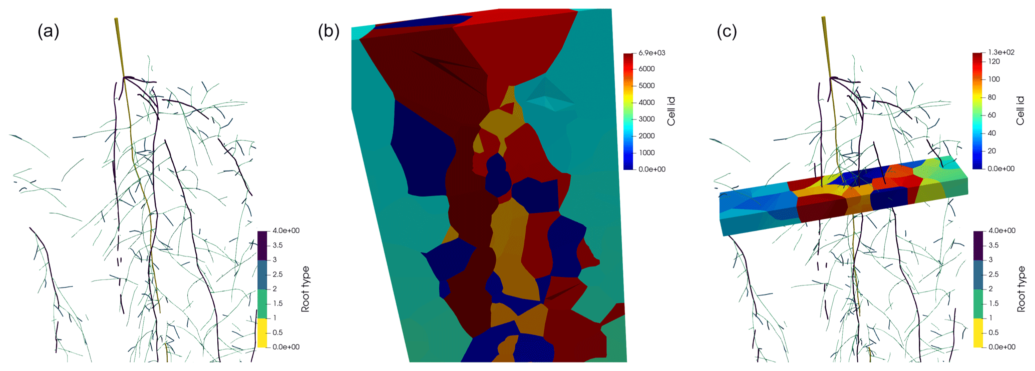
Figure 3 Panel (a) shows the spring barley root system mapped to a periodic domain. Panel (b) shows the Voronoi diagram bounded by the periodic domain, where each Voronoi cell is located around a node. Panel (c) shows the Voronoi diagram of a single layer with 1 cm height.

In the first approach, we use a 3D Voronoi mesh around the nodes of the root system considering all lateral roots. In this way, the soil volume is partitioned into cells, where each node has a corresponding Voronoi cell; see Fig. 3. The Voronoi cell faces are located at mid-distance between the neighbouring nodes. Therefore, the volume of the Voronoi cells is a good approximation of the node perirhizal volume, and we define the root segment's perirhizal volume vol_j (cm³) as the volume of the Voronoi cell of the segment's apical node. We approximate this volume by a cylindrical geometry of the same volume, i.e.

$$\begin{array}{}\text{(28)}& {\text{vol}}_j=\mathit{\pi }{l}_{\mathrm{root},j}(a_{\mathrm{prhiz},j}^{\mathrm{2}}-a_{\mathrm{root},j}^{\mathrm{2}}),\end{array}$$

and we can calculate the outer perirhizal radius a_prhiz,j for each root segment j as

$$\begin{array}{}\text{(29)}& a_{\mathrm{prhiz},j}=\sqrt{{\displaystyle \frac{{\text{vol}}_j}{\mathit{\pi }{l}_{\mathrm{root},j}}}+a_{\mathrm{root},j}^{\mathrm{2}}}.\end{array}$$

The more commonly used approach so far is to approximate the perirhizal geometry using root length density (cm cm⁻³), surface density (cm² cm⁻³), or volume density (cm³ cm⁻³) in a finite soil volume vol_soil (cm³) (e.g. De Bauw et al., 2020; Mai et al., 2019). Assuming that the roots are evenly distributed, the perirhizal volume is given by

$$\begin{array}{}\text{(30)}& {\text{vol}}_j=t_j{\text{vol}}_{\mathrm{soil}},\end{array}$$

where t_j (1) is the ratio between the segment length (or surface or volume) and the total root length (or surface or volume) within the finite soil volume. The outer radius a_prhiz,j for each root segment j is again given by Eq. (29).

If we couple the perirhizal models with a macroscopic soil model, the Voronoi mesh or the density-based method must be aligned with the macroscopic finite volume cells for mass conservation. For both methods, this will affect the distribution of perirhizal radii; see Sect. 3.2. This density-based approach is suitable for soils where the soil grid cells are 3D with edge length in the order of centimetres. For 1D layered soil grids, the Voronoi-mesh-based method is preferable, allowing more realistic distributions of the true perirhizal zones within each soil layer. Note that both approaches are approximations, since we assume a cylindrical perirhizal zone, which is generally not the case. The Voronoi method computes more realistic perirhizal volumes but is computational expensive and less feasible for dynamic root growth.

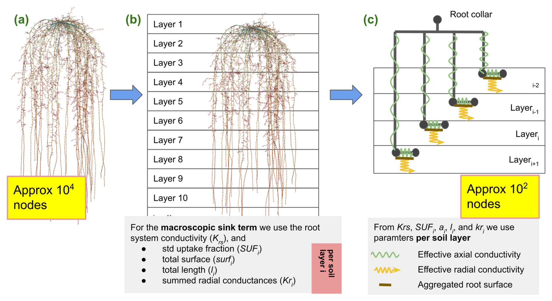
Figure 4 Starting from the full hydraulic model, panel (a), we first derive the root system conductance K_rs and layer aggregated root hydraulic root properties, panel (b). These are given for each soil layer or soil volume i as ${\text{SUF}}_i^{\mathrm{ups}}$, total root surface $\mathit{s}\mathit{u}\mathit{r}{\mathit{f}}_i^{\mathrm{ups}}$, total summed length $l_i^{\mathrm{ups}}$, and mean radial conductivity $K_{\mathrm{r},i}^{\mathrm{ups}}$. In a final step, panel (c), we neglect the actual root architecture and replace it with a parallel root system with hydraulic parameters, preserving the macroscopic hydraulic properties.

2.5 Upscaling by aggregating RWU from root segment to soil element level (Bxx)

For developing larger-scale models, we want to describe the effect of the root system without keeping track of the exact root system geometry. Generally, the number of root segments is much higher than the number of finite soil volumes for 1D, 2D, or 3D soil models. Therefore, we aim for models that are described on the soil element level. These models are of category Bxx.

The linear system in Eq. (18) describes one equation per root node excluding the root collar, i.e. n−1 equations. The number of soil cells m is generally much lower $m\ll n-\mathrm{1}$, and we will rewrite the linear system in variables given per soil cell. We can sum up Eq. (17) regarding the soil cells by multiplying with the matrix M, i.e.

$$\begin{array}{}\text{(31)}& \begin{array}{rl}\mathbf{M}{\mathit{q}}_{\mathrm{root}}& =\mathbf{M}\text{diag}\left({\mathit{K}}_{\mathrm{r}}\right)(\mathbf{I}-{\mathbf{A}}^{-\mathrm{1}}\text{diag}({\mathit{K}}_{\mathrm{r}}\left)\right){\mathit{H}}_{\mathrm{sr}}\\ & -\mathbf{M}\text{diag}\left({\mathit{K}}_{\mathrm{r}}\right){\mathbf{A}}^{-\mathrm{1}}{k}_{x,\mathrm{1}}{\mathit{e}}_{\mathrm{1}}{\mathit{H}}_{\mathrm{collar}},\end{array}\end{array}$$

where M is an $m\times (n-\mathrm{1})$ matrix mapping each root node index to a soil cell index. For each column (i.e. node index-1) the matrix contains exactly a 1 in the row of the soil cell index where the node is located and zero otherwise. Therefore, the RWU from a soil volume q_soil (cm³ d⁻¹) is given by

$$\begin{array}{}\text{(32)}& {\mathit{q}}_{\mathrm{soil}}=\mathbf{M}{\mathit{q}}_{\mathrm{root}},\end{array}$$

and the right-hand side of Eq. (31) exactly computes the soil fluxes. Now, we can simplify the system by assuming that the soil–root matric potential is the same in each soil cell.

We define ${\mathit{H}}_{\mathrm{sr}}^{\mathrm{soil}}\in {\mathbb{R}}^m$ to be the mean value of the H_sr in each soil volume. Note that (M M^T) is an m×m diagonal matrix containing the number of root nodes within each soil cell; therefore the mean value is given by

$$\begin{array}{}\text{(33)}& {\mathit{H}}_{\mathrm{sr}}^{\mathrm{soil}}:=(\mathbf{M}{\mathbf{M}}^T{)}^{-\mathrm{1}}\mathbf{M}{\mathit{H}}_{\mathrm{sr}}=({\mathbf{M}}^T{)}^{+}{\mathit{H}}_{\mathrm{sr}},\end{array}$$

where M^T+ is the Moore–Penrose pseudo-inverse of M^T. We can approximately solve above the equation for H_sr, yielding

$$\begin{array}{}\text{(34)}& {\mathbf{M}}^T{\mathit{H}}_{\mathrm{sr}}^{\mathrm{soil}}\approx {\mathit{H}}_{\mathrm{sr}},\end{array}$$

where M^T is an n×m matrix, ${\mathit{H}}_{\mathrm{sr}}^{\mathrm{soil}}$ is an m dimensional vector at soil element level, and H_sr is an n dimensional vector at root segment level. Note that, in this case, all entries of H_sr will be the same within every soil element, and this assumption causes loss of information.

Inserting the approximation of Eq. (34) into Eq. (31) yields

$$\begin{array}{}\text{(35)}& \begin{array}{rl}{\mathit{q}}_{\mathrm{soil}}& =\underset{{\mathbf{A}}_{\mathrm{up}}\in {\mathbb{R}}^{m\times m}}{\underbrace{\mathbf{M}\text{diag}\left({\mathit{K}}_{\mathrm{r}}\right)(\mathbf{I}-{\mathbf{A}}^{-\mathrm{1}}\text{diag}({\mathit{K}}_{\mathrm{r}}\left)\right){\mathbf{M}}^T}}\\ & \cdot {\mathit{H}}_{\mathrm{sr}}^{\mathrm{soil}}-\underset{{\mathit{b}}_{\mathrm{up}}\in {\mathbb{R}}^m}{\underbrace{\mathbf{M}\text{diag}\left({\mathit{K}}_{\mathrm{r}}\right){\mathbf{A}}^{-\mathrm{1}}{k}_{x,\mathrm{1}}{\mathit{e}}_{\mathrm{1}}{\mathit{H}}_{\mathrm{collar}}}}.\end{array}\end{array}$$

This much smaller linear system can be solved very quickly after calculating A_up once. However, the number of root nodes might be limiting, since it is necessary to explicitly calculate A⁻¹.

For including the perirhizal model in the aggregated approach (Eq. 35), the total potential ${\mathit{H}}_x^{\mathrm{soil}}$ can be calculated from q_soil summing up Eq. (11) over the soil cells:

$$\begin{array}{}\text{(36)}& {\displaystyle }\mathbf{M}{\mathit{q}}_{\mathrm{root}}=\mathbf{M}\text{diag}\left({\mathit{K}}_{\mathrm{r}}\right)({\mathit{H}}_{\mathrm{sr}}-{\mathit{H}}_x),\text{(37)}& {\displaystyle }\mathbf{M}{\mathit{q}}_{\mathrm{root}}=\mathbf{M}\left(\text{diag}\right({\mathit{K}}_{\mathrm{r}}{)}^{-\mathrm{1}}+\text{diag}\left({\mathbf{K}}_{\mathrm{prhiz}}{)}^{-\mathrm{1}}{)}^{-\mathrm{1}}\right({\mathit{H}}_{\mathrm{s}}-{\mathit{H}}_x),\text{(38)}& {\displaystyle }{\mathit{q}}_{\mathrm{soil}}=\mathbf{M}\text{diag}\left({\mathit{K}}_{\mathrm{r}}\right)({\mathbf{M}}^T{\mathit{H}}_{\mathrm{sr}}^{\mathrm{soil}}-{\mathbf{M}}^T{\mathit{H}}_x^{\mathrm{soil}}),\text{yielding}\text{(39)}& {\displaystyle }{\mathit{H}}_x^{\mathrm{soil}}={\mathit{H}}_{\mathrm{sr}}^{\mathrm{soil}}-(\underset{{\mathbf{K}}_{\mathrm{r},\mathrm{up}}\in {\mathbb{R}}^{m\times m}}{\underbrace{\mathbf{M}\text{diag}\left({\mathit{K}}_{\mathrm{r}}\right){\mathbf{M}}^T}}{)}^{-\mathrm{1}}{\mathit{q}}_{\mathrm{soil}}.\end{array}$$

Therefore, the soil total potential can be represented by the potentials at the perirhizal interfaces subtracted by the soil flux.

A suitable pair, ${\mathit{H}}_x^{\mathrm{soil}}$ and ${\mathit{H}}_{\mathrm{sr}}^{\mathrm{soil}}$ (both on soil element level), is found using a fixed-point iteration as before for values per segment (Algorithm 2).

Algorithm 2 Fixed-point iteration to find consistent values ${\mathit{H}}_x^{\mathrm{soil}}$ and ${\mathit{H}}_{\mathrm{sr}}^{\mathrm{soil}}$.

Initialize: k:=0, ${\mathit{H}}_x^{\mathrm{soil},\mathrm{0}}:=h_{\mathrm{soil}}\left({\mathit{q}}_{\mathrm{soil}}\right({\mathit{H}}_{\mathrm{sr}}^{\mathrm{soil},\mathrm{prev}}\left)\right)$, applying Eq. (35) first and then Eq. (39).

(1)

${\mathit{H}}_{\mathrm{sr}}^{\mathrm{soil},k+\mathrm{1}}:=f_{\mathrm{prhiz}}({\mathit{H}}_x^{\mathrm{soil},k},{\mathit{H}}_{\mathrm{s}})$, Eq. (27), with averaged root and perirhizal radii per soil volume (3D) or soil layer (1D).

(2)

${\mathit{H}}_x^{\mathrm{soil},k+\mathrm{1}}:=h_{\mathrm{soil}}\left({\mathit{q}}_{\mathrm{soil}}\right({\mathit{H}}_{\mathrm{sr}}^{\mathrm{soil},k}\left)\right)$, applying Eq. (35) first and then Eq. (39).

(3)

$k:=k+\mathrm{1}$, proceed with Step (1), until ${\mathit{H}}_x^{\mathrm{soil},k+\mathrm{1}}\approx {\mathit{H}}_x^{\mathrm{soil},k}$ and ${\mathit{H}}_{\mathrm{sr}}^{\mathrm{soil},k+\mathrm{1}}\approx {\mathit{H}}_{\mathrm{sr}}^{\mathrm{soil},k}$.

2.6 Upscaling by root architecture simplification: the parallel root system approach (Cxx)

In a further simplification step, we replace the exact root system by a parallel root system, where we assume exactly one single-root segment per soil element (Vanderborght et al., 2021). Each of these segments is connected directly to the root collar by an artificial root segment; see Fig. 4. The RWU of such a system is described by

$$\begin{array}{}\text{(40)}& {\mathit{q}}_{\mathrm{soil}}=K_{\mathrm{rs}}\text{diag}\left(\mathit{S}\mathit{U}{\mathit{F}}^{\mathrm{ups}}\right)({\mathit{H}}_{\mathrm{sr}}^{\mathrm{ups}}-{\mathit{H}}_{\mathrm{collar}}),\end{array}$$

where q_soil is the RWU per soil volume (cm³ d⁻¹), K_rs the standard uptake fraction, ${\mathit{H}}_{\mathrm{sr}}^{\mathrm{ups}}$ is the total potential at the soil–root interface (cm), and H_collar is a vector where each component is the total water potential at root collar (cm).

Root hydraulic parameters of the parallel root model are chosen in a way that the macroscopic hydraulic properties of the exact root system are preserved. These properties are the root system conductance K_rs (cm² d⁻¹), the standard uptake fraction SUF^ups (1), the total root length l^ups (cm), the total root surface surf^ups (cm²), and the root radial conductance ${\mathit{K}}_{\mathrm{r}}^{\mathrm{ups}}$ (cm² d⁻¹) per each soil element. These models are of category Cxx. This model is simpler than Bxx, as the general incidence matrix representing the hydraulic root architecture and mapped to the soil elements is replaced by a simple diagonal matrix. This results in a computationally less expensive simulation at the cost of loss of accuracy, particularly noticeable for highly heterogeneous soil water potential, as hydraulic lift can only occur via a “detour” via the root collar.

Firstly, we obtain SUF^ups, root length ${\mathit{l}}_{\mathrm{root}}^{\mathrm{ups}}$, surface surf^ups, and root radial conductance ${\mathit{K}}_{\mathrm{r}}^{\mathrm{ups}}$ per soil element by summing the corresponding values given per each root segment over each soil layer or soil volume,

$$\begin{array}{}\text{(41)}& {\displaystyle }\mathit{S}\mathit{U}{\mathit{F}}^{\mathrm{ups}}:=\mathbf{M}\mathit{S}\mathit{U}\mathit{F},\text{(42)}& {\displaystyle }{\mathit{l}}_{\mathrm{root}}^{\mathrm{ups}}:=\mathbf{M}{\mathit{l}}_{\mathrm{root}},\text{(43)}& {\displaystyle }\mathit{s}\mathit{u}\mathit{r}{\mathit{f}}^{\mathrm{ups}}:=\mathbf{M}\mathit{s}\mathit{u}\mathit{r}\mathit{f},\text{(44)}& {\displaystyle }{\mathit{K}}_{\mathrm{r}}^{\mathrm{ups}}:=\mathbf{M}{\mathit{K}}_{\mathrm{r}},\end{array}$$

where M is an $m\times (n-\mathrm{1})$ matrix mapping each root node index to a soil cell index as described in the previous section. Therefore, SUF^ups, ${\mathit{l}}_{\mathrm{root}}^{\mathrm{ups}}$, a^ups, and ${\mathit{K}}_{\mathrm{r}}^{\mathrm{ups}}$ are m×1 vectors, where m is the number of soil layers.

Next, we choose the axial conductance ${\mathit{K}}_x^{\mathrm{ups}}$ of the artificial segments, which connects the single-root segments to the collar in such a way that the macroscopic root system hydraulic properties SUF and K_rs are the same as in the exact hydraulic model. For each soil layer, the RWU can be described as

$$\begin{array}{}\text{(45)}& {\displaystyle }({\mathit{q}}^{\mathrm{soil}}{)}_i& {\displaystyle }=K_{\mathrm{rs}}{\text{SUF}}_i^{\mathrm{ups}}\left(({\mathit{H}}_{\mathrm{sr}}^{\mathrm{ups}}{)}_i-H_{\mathrm{collar}}\right),\text{(46)}& {\displaystyle }& {\displaystyle }=K_{\mathrm{r},i}^{\mathrm{ups}}\left(({\mathit{H}}_{\mathrm{sr}}^{\mathrm{ups}}{)}_i-({\mathit{H}}_x^{\mathrm{ups}}{)}_i\right),\text{(47)}& {\displaystyle }& {\displaystyle }=K_{x,i}^{\mathrm{ups}}\left(({\mathit{H}}_x^{\mathrm{ups}}{)}_i-H_{\mathrm{collar}}\right),\end{array}$$

where ${\mathit{H}}_x^{\mathrm{ups}}$ is the total xylem potential of the parallel root system model (cm). From these equations, we can we calculate ${\mathit{K}}_x^{\mathrm{ups}}$ as

$$\begin{array}{}\text{(48)}& ({\mathit{K}}_x^{\mathrm{ups}}{)}_i={\displaystyle \frac{K_{\mathrm{rs}}{\text{SUF}}_i^{\mathrm{ups}}}{\mathrm{1}-K_{\mathrm{rs}}{\text{SUF}}_i^{\mathrm{ups}}/K_{\mathrm{r},i}^{\mathrm{ups}}}},\end{array}$$

using $K_{\mathrm{rs}}{\text{SUF}}_i/K_{\mathrm{r},i}^{\mathrm{ups}}=(H_{\mathrm{sr},i}^{\mathrm{ups}}-H_{x,i}^{\mathrm{ups}})/(H_{\mathrm{sr},i}^{\mathrm{ups}}-{\mathit{H}}_{\mathrm{collar}})$ from Eqs. (45) and (46).

We use the same iteration as in Algorithm 1, but the exact root architecture is replaced by the parallel root model. We iterate to find a suitable pair of ${\mathit{H}}_{\mathrm{sr}}^{\mathrm{ups}}$ and ${\mathit{H}}_x^{\mathrm{ups}}$.

Algorithm 3 Fixed-point iteration to find consistent values ${\mathit{H}}_{\mathrm{sr}}^{\mathrm{ups}}$ and ${\mathit{H}}_x^{\mathrm{ups}}$.

Initialize: k:=0, ${\mathit{H}}_x^{\mathrm{ups},\mathrm{0}}:=f_{\mathrm{root}}\left({\mathit{H}}_{\mathrm{sr}}^{\mathrm{ups},\mathrm{prev}}\right)$; see Eq. (15).

(1)

${\mathit{H}}_{\mathrm{sr}}^{\mathrm{ups},k+\mathrm{1}}:=f_{\mathrm{prhiz}}({\mathit{H}}_x^{\mathrm{ups},k},{\mathit{H}}_{\mathrm{s}}^{\mathrm{ups}})$; see Eq. (27).

(2)

${\mathit{H}}_x^{\mathrm{ups},k+\mathrm{1}}:=f_{\mathrm{root}}\left({\mathit{H}}_{\mathrm{sr}}^{\mathrm{ups},k}\right)$, see Eq. (15)

(3)

$k:=k+\mathrm{1}$ and proceed with Step (1) until ${\mathit{H}}_x^{\mathrm{ups},k+\mathrm{1}}\approx {\mathit{H}}_x^{\mathrm{ups},k}$ and ${\mathit{H}}_{\mathrm{sr}}^{\mathrm{ups},k+\mathrm{1}}\approx {\mathit{H}}_{\mathrm{sr}}^{\mathrm{ups},k}$.

With the parallel root system approach, the exact root architecture and hydraulic properties can be neglected, while K_rs and SUF^ups are still preserved. The simplified model is typically much faster to solve, having less than 1 % of the degrees of freedom of the original root system. Furthermore, root hydraulics are solely dependent on the parameters K_rs, l^ups, a^ups, and ${\mathit{K}}_{\mathrm{r}}^{\mathrm{ups}}$, which are much easier to handle compared to the full hydraulic model. At a constant total soil potential, the approximation will be exact, but we expect differences in dynamic settings where strong variations in soil potential can appear.

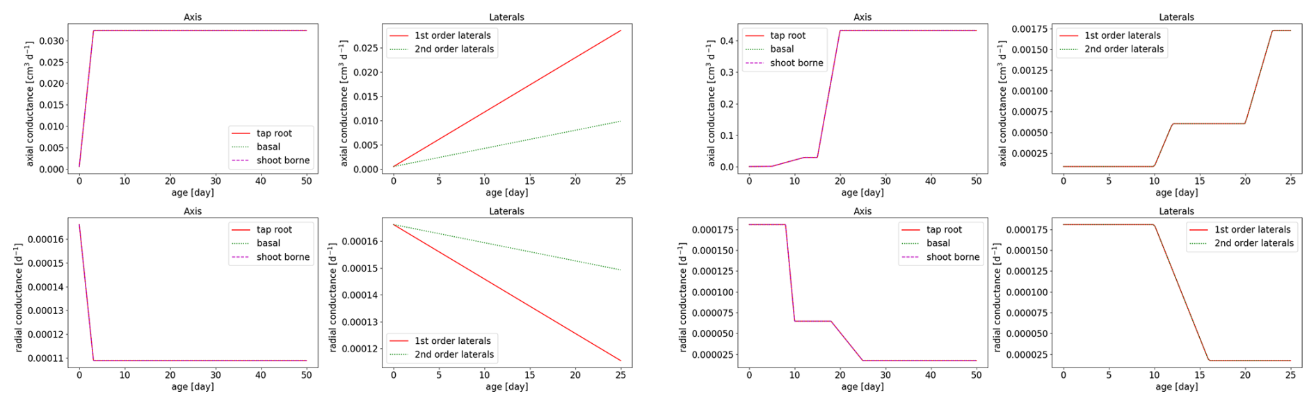
Figure 5 The age-dependent root axial conductances and radial conductivities for spring barley (left subplot) and maize (right subplot).

2.7 Root soil hydraulic scenarios

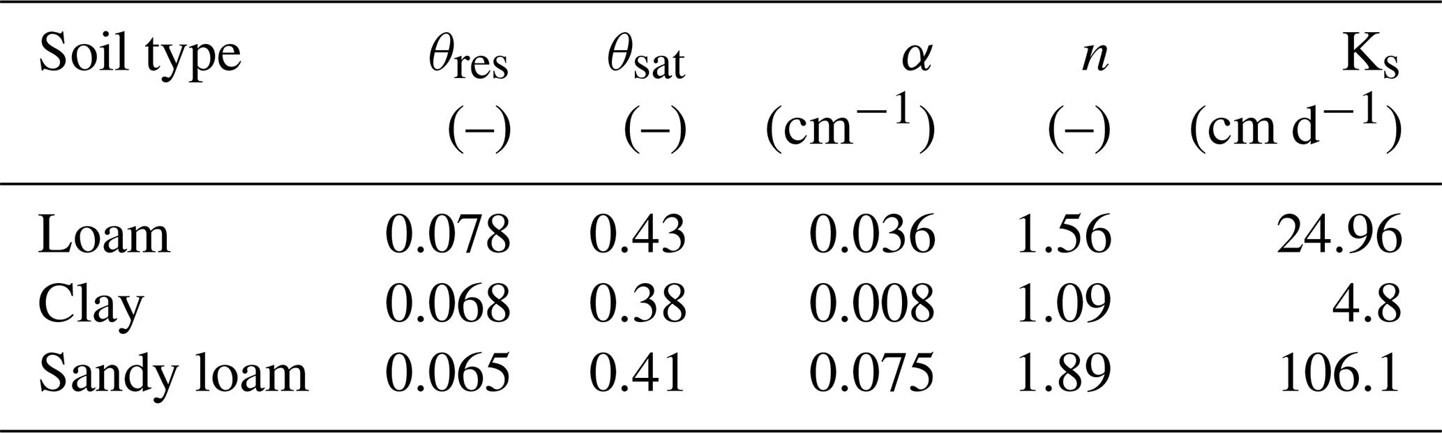
Root hydraulic properties are given by the root radial and root axial conductances. These values were taken from the literature: Knipfer and Fricke (2010) for spring barley using linear regression and Couvreur et al. (2012) for maize. The hydraulic properties depend on the age of the root segments; see Fig. 5. For both measurements, axial conductances increase with root age, while radial conductances decrease. Soil hydraulic properties were described by the Van Genuchten model (Van Genuchten, 1980). We obtained typical parameters for loam, clay, and sandy loam using the Hydrus 1D soil catalogue (Simunek et al., 2005); see Table 2.

Table 2 Van Genuchten parameters for loam, clay, and sandy loam from the Hydrus 1D soil catalogue (Simunek et al., 2005).

In order to simulate field conditions, we consider the root architectures of spring barley and maize in a periodic domain. In this way, we have two contrasting setups: for spring barley, we choose an inter-row distance of 13 cm and plant spacing of 3 cm; for maize, we choose a larger inter-row distance of 76 cm and plant spacing of 16 cm. We consider both plants at the end of their vegetative stage, resulting in a growth period of 7 weeks for spring barley and 8 weeks for maize.

All the following scenarios include nonlinear conductivities from the perirhizal model. The simulations describe water depletion from an initially wet soil of −200 cm total soil water potential using a transpiration rate of 0.5 (cm d⁻¹) with a sinusoidal shape from 06:00 to 18:00 LT with maximal transpiration at noon and no uptake during the night. Actual RWU and corresponding cumulative uptake is calculated over 2 weeks. At the top and bottom of the soil domain, we prescribe no-flux boundary conditions so that water can leave the domain only through transpiration. In the 3D scenarios, the boundary conditions at the sides are periodic.

3 Results

In the following, we first present the simulation results of root architecture and the corresponding precomputed perirhizal outer radii. Then, we show simulation results of the root hydraulic models using the dynamic scenarios presented in Sect. 2.7. The implementation of the new upscaled models was performed in the framework of CPlantBox (https://github.com/Plant-Root-Soil-Interactions-Modelling/CPlantBox, last access: 30 December 2024) and dumux-rosi (https://github.com/Plant-Root-Soil-Interactions-Modelling/dumux-rosi, last access: 30 December 2024), and the following results can be found in the branch “upscaling”.

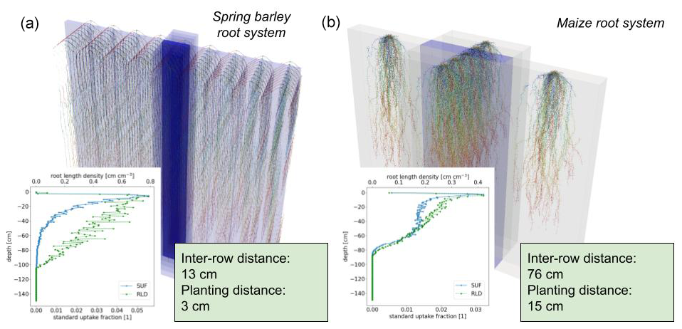
Figure 6 Spring barley (a) and maize (b) root architecture under field conditions, both at the end of their vegetative stage (after 7 weeks for spring barley and 8 weeks for maize). In the lower-left subplots, we show the corresponding SUF and root length density (RLD).

3.1 Root architectures for spring barley and maize

Figure 6 shows the root architecture development after 7 weeks for spring barley and after 8 weeks for maize, and it illustrates the concept of using periodicity to mimic field conditions. The axial resolution of the roots is set to a maximum of 0.5 cm, yielding a final amount of 6.92×10³ nodes for the spring barley and 4.82×10⁴ segments for the maize root system.

From root topology and root hydraulic parameters at segment level (see Sect. 2.7), we calculated the macroscopic root system hydraulic parameters K_rs, SUF; see lower-left subplots in Fig. 6. Spring barley has a K_rs of 0.0064 (cm² d⁻¹), and maize has a K_rs of 0.1345 (cm² d⁻¹).

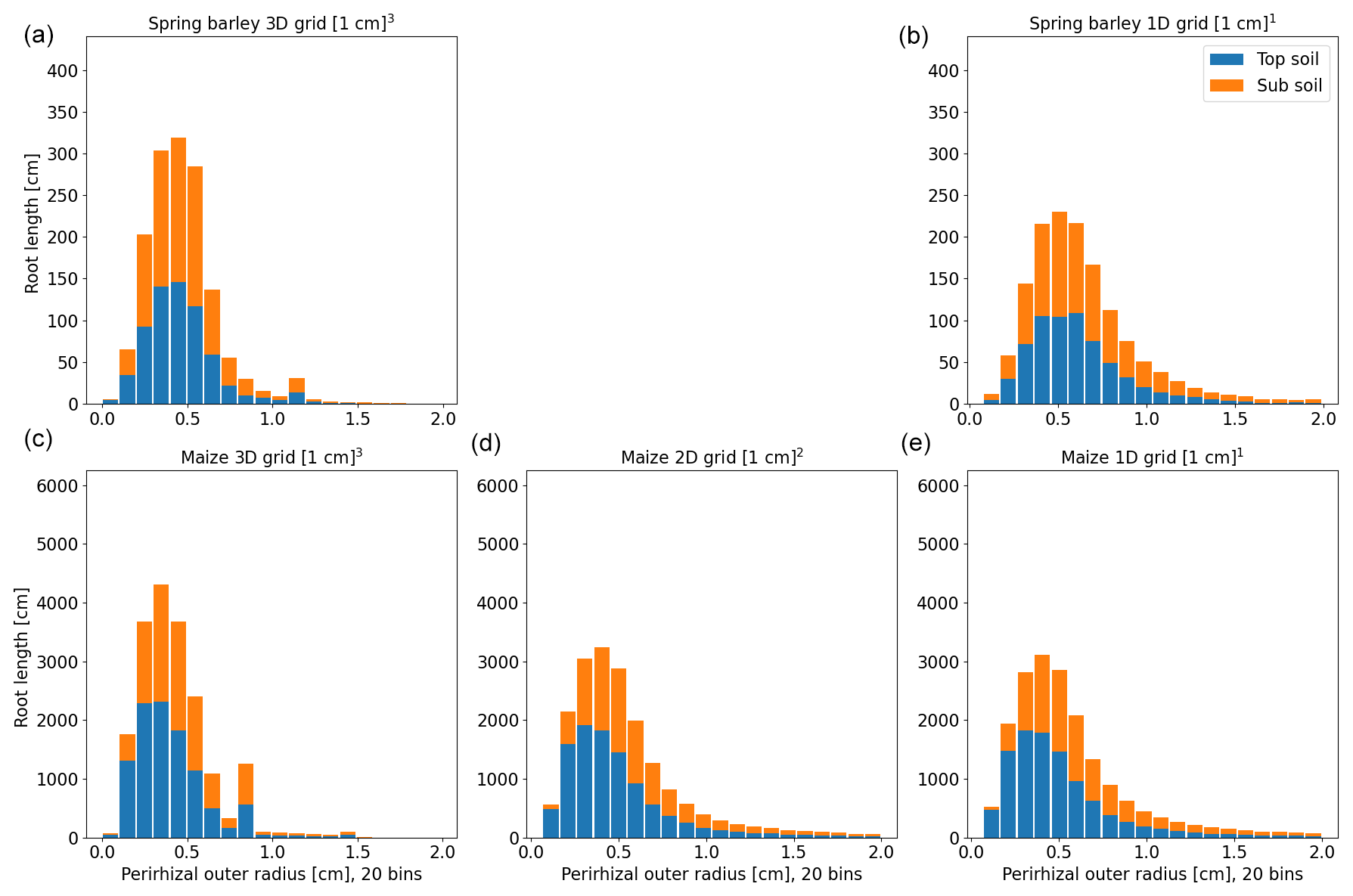
Figure 7 Histogram of perirhizal zone outer radii using a 3D Voronoi diagram for spring barley (a, b) and maize (c–e) for the soil grids used in the following sections. Colours denote typical soil horizons: topsoil 0–30 cm depth and subsoil 30–150 cm depth.

3.2 Perirhizal outer radii

Perirhizal outer radii are precomputed for both root systems. The first approach (xAx; see Sect. 2.4) is to use a Voronoi mesh that is aligned to the soil grids; i.e. the maximum Voronoi cell volume is equal to soil cell volume. Figure 7 shows the distribution of perirhizal outer radii with a topsoil depth of 0–30 cm and a subsoil depth of 30–150 cm. Note that the perirhizal radius can be larger than $\sqrt{{\text{vol}}_{\mathrm{soil}}/\mathit{\pi }}$ if the root segment length is small; see Eq. (29). In both root architectures, root density in the topsoil is higher, leading to a smaller mean outer perirhizal radius in the topsoil. For spring barley, the mean outer radius is 0.51 cm (3D) and 0.71 cm (1D) in topsoil and 0.53 cm (3D) and 0.92 cm (1D) in subsoil; for maize, it is 0.47 cm (3D), 0.65 cm (2D), and 0.75 cm (1D) in topsoil and 0.55 cm (3D), 0.92 cm (2D), and 1.14 cm (1D) in subsoil. A reduction in the dimensions of the soil grid generally leads to higher mean outer perirhizal radii.

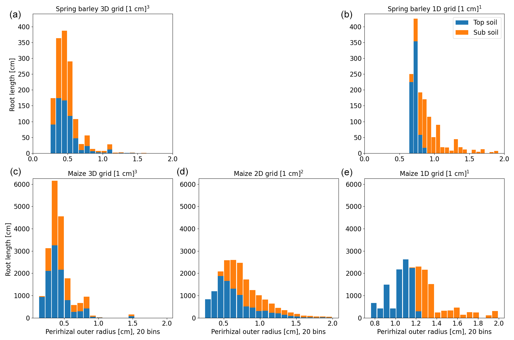
Figure 8 Histogram of perirhizal zone outer radii using root length densities to obtain perirhizal outer radii for spring barley (a, b) and maize (c–e) for the soil grids used in the following sections. Colours denote typical soil horizons: topsoil 0–30 cm depth and subsoil 30–150 cm depth.

The second approach (xBx; see Sect. 2.4) uses root length, surface, or volume densities to compute the perirhizal outer radii. Figure 8 shows the distribution of perirhizal outer radii in topsoil and subsoil based on length densities for the soil grid types used in the simulations. As for the Voronoi method, topsoil mean outer radii are smaller due to higher root density: 0.43 cm (3D) and 0.72 cm (1D) for spring barley and 0.42 cm (3D), 0.65 cm (2D), and 1.05 cm (1D) for maize. For subsoil, mean radii are 0.51 cm (3D) and 1.02 cm (1D) for spring barley and 0.49 cm (3D), 0.93 cm (2D), and 1.5 cm (1D) for maize. For the 1D soil layers, the histogram is strongly divided into radii classes because of the limited number of soil layers, where most smaller outer radii are located in the upper layers. For 1D soil grids, we expect the largest deviation in model results compared to using the Voronoi method.

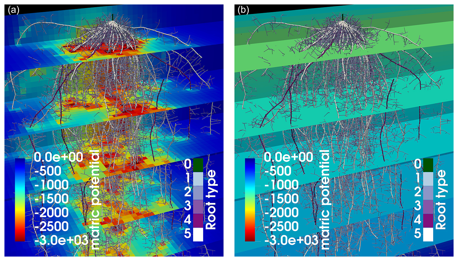
Figure 9 Soil matric potential for maize in loam soil after 2 weeks of simulation time in a 3D grid (a) and in a 1D grid (b). In panel (a), local depletion develops around areas with high RLD, while, in panel (b), the water potential is constant per soil layer.

3.3 Root soil hydraulic simulation results

3.3.1 Full hydraulic model using a 3D grid (AAA) compared to a lower-dimensional grid (AAB)

The full hydraulic 3D model is solved as described in Sect. 2.3, and perirhizal radii were determined using the Voronoi method (see Sect. 2.4) for the scenarios presented in Sect. 2.7. We compare using a 3D macroscopic soil with a resolution of 1 cm³ (reference scenario AAA) to using a 1D macroscopic soil with layers of 1 cm thickness (AAB), where only the vertical water movement is considered. Figure 9 shows the resulting soil matric potential for maize in loam soil after 2 weeks of simulation time and highlights the difference between the 3D grid and the 1D grid where horizontal water movement is neglected. Using a 3D grid (left subplot) shows the development of local water depletion around areas with high RLD, while using a 1D grid (right subplot) relies on averaged values per layer.

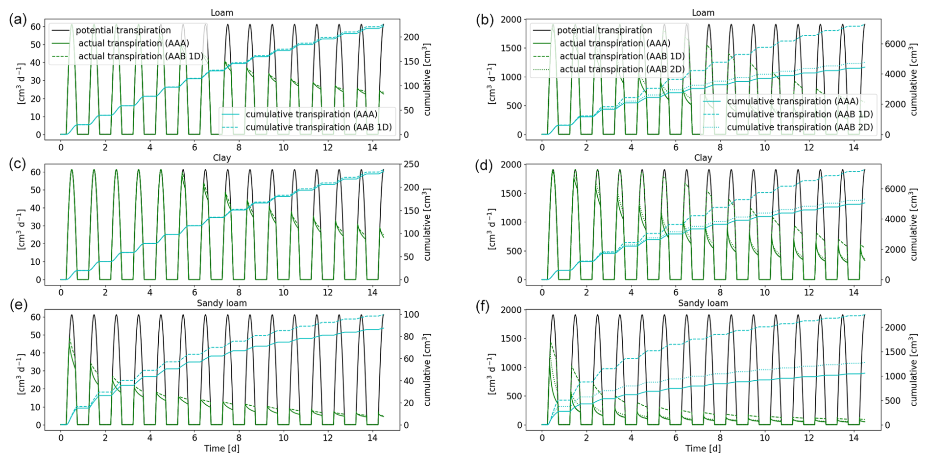
Figure 10 Potential and actual transpiration of the full 3D hydraulic model of spring barley (a, c, e) and maize (b, d, f) for the soil types loam (a, b), clay (c, d), and sandy loam (e, f). The blue line indicates the cumulative plant water uptake. Solid lines represent the results using a 3D soil grid (AAA), while dashed lines are the results using a 1D grid and dotted lines are the results using a 2D grid (AAB).

The actual and cumulative transpiration is presented in Fig. 10 for the three soil types. The solid curve represents the reference scenario (AAA), and the dashed line represents the scenario using a 1D macroscopic soil grid (AAB). Additionally, for maize, the dotted line shows the solution using a 2D macroscopic grid, where water movement along the plant rows is neglected. Generally, for maize, water stress occurred earlier compared to spring barley for loam and clay. For sandy loam, both root systems were immediately in stress. The differences in cumulative root uptake are much higher for maize, since there is more variation in RLD due to the distance between the planting rows. Using a 2D macroscopic grid, where water movement in this direction is enabled, yields an improved accuracy. For spring barley, RLD is much more uniform due to smaller planting distances; therefore the error by neglecting lateral water movement is small. Additionally, the differences are smaller in finer-textured soils, since they redistribute the water over larger distances so that the soil water potential is more uniform.

A lower-dimensional soil grid leads to an overestimation in RWU compared to the full 3D model. For spring barley, after 1 week, the cumulative root uptake differed by 1 % for loam, 0.7 % for clay, and 12.5 % for sandy loam; after 2 weeks, the error increased to 1.6 % for loam, 1.7 % for clay, and 13.9 % for sandy loam. For maize, cumulative transpiration is largely overestimated using a 1D soil grid. After 1 week simulation time, it differed by 43.5 % for loam, 28.1 % for clay, and 115.1 % for sandy loam; after 2 weeks, it differed by 62.4 % for loam, 42.5 % for clay, and 110.8 % for sandy loam. Using a 2D soil grid, errors for maize reduced to 13.3 % for loam, 8 % for clay, and 45.5 % for sandy loam after 1 week and 13.4 %, 8.4 %, and 34.9 % after 2 weeks.

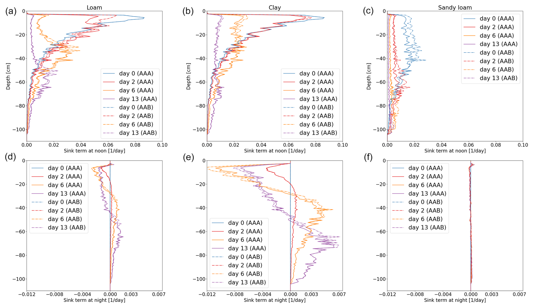
Figure 11 Vertical RWU of the full hydraulic 3D model during noon (a–c) and redistribution during the night (d–f) of spring barley for loam (a, d), clay (b, e), and sandy loam (c, f). Solid lines represent the results using a 3D soil grid (AAA), while dashed lines use a 1D grid (AAB).

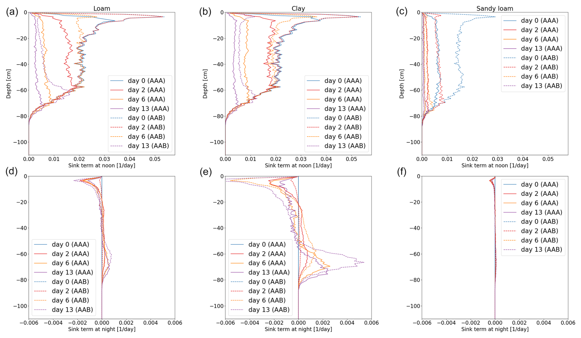
Figure 12 Vertical RWU of the full hydraulic 3D model during noon (a–c) and redistribution during the night (d–f) of maize for loam (a, d), clay (b, e), and sandy loam (c, f). Solid lines represent the results using a 3D soil grid (AAA), while dashed lines use a 1D grid (AAB).

Figures 11 and 12 show the RWU of spring barley and maize from soil at noon (top row) and redistribution during the night (bottom row) for the three soil types. Solid lines represent the results using a 3D soil grid (AAA), while dashed lines use a 1D grid (AAB). The different root architectures result in different RWU patterns. In the beginning (blue line), the RWU is proportional to the SUF, since the initial total soil water potential is constant. Firstly, water is taken up from the upper layers; later, when the upper layer becomes drier, more water is taken up from the lower layers, qualitatively changing the shape of the RWU profile. During the night, water is redistributed from the lower layers into the upper layers. Redistribution is strongest for clay for both spring barley and maize and is negligible for sandy loam.

Using a 1D soil grid leads to differences in RWU patterns: for spring barley, the differences are small in all soil types over the whole period of 2 weeks. Differences in maize are strong due to the overestimated cumulative transpiration (see the right column of Fig. 10), which also impacts the local uptake. For loam and clay soil, uptake from the upper layer is largely overestimated at the beginning, leading to a delayed dynamic in water uptake and redistribution. For loam and clay, the RWU is proportional to the SUF for the first 2 d until the profile changes due to soil water depletion in the upper layers.

While introducing errors, computational time decreases. For spring barley, the model runs 5 times faster for loam and clay and 3 times faster for sandy loam. For maize, the speed-up compared to the 3D soil grid is higher, since the 3D domain is larger, yielding a speed-up of 15 times for loam, 18 times for clay, and 11 times for sandy loam for the 1D grid and 8 times for loam and clay and 10 times for sandy loam for the 2D grid.

3.3.2 The impact of using density-based outer perirhizal radii instead of the Voronoi method (AAA vs. ABA; AAB vs. ABB)

We compare the full hydraulic model using the 3D macroscopic soil and the Voronoi method for the outer perirhizal radii (AAA) to the same model, where the outer radii were based on root length, surface, or volume (ABA). Actual transpiration and the shape and dynamics of the resulting RWU were similar, and errors of cumulative transpiration were under 1 % after 2 weeks. Given their similarities, this information is not plotted.

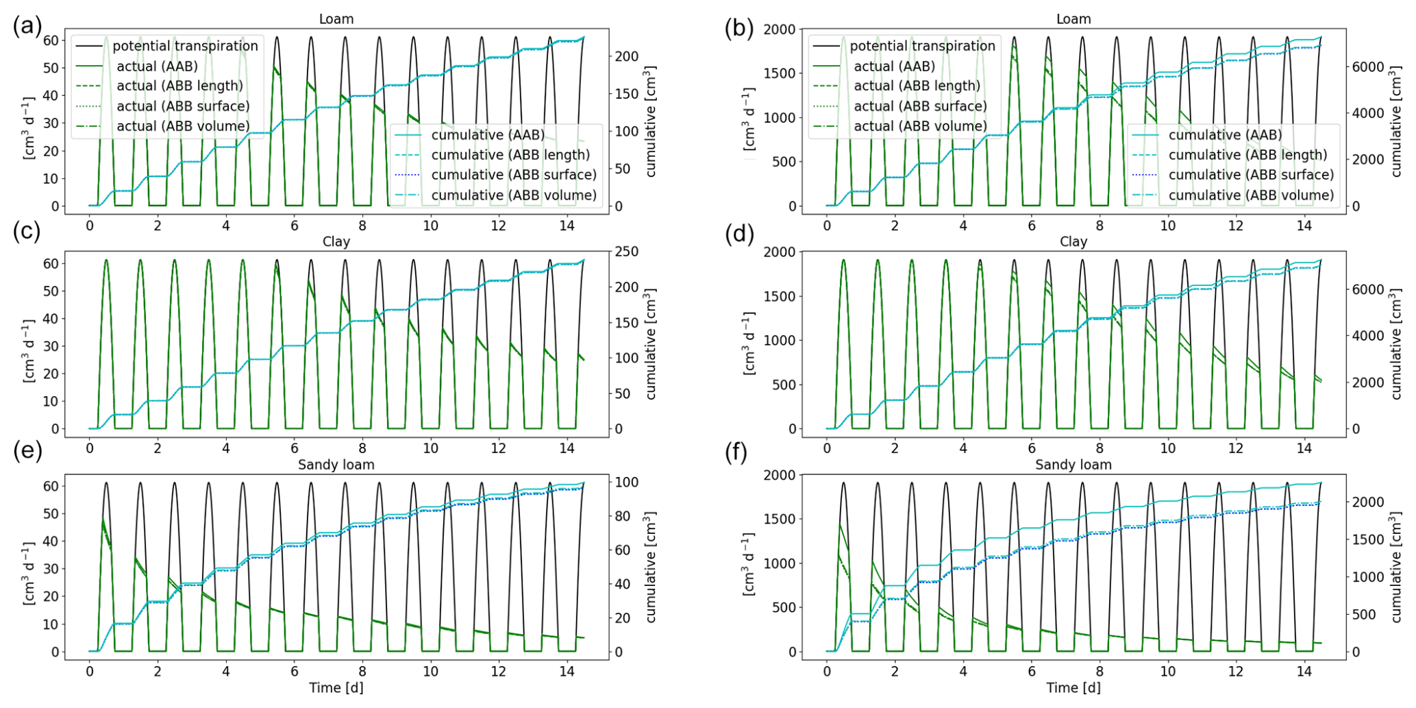
Figure 13 Potential and actual transpiration of the full hydraulic 3D model of spring barley (a, c, e) and maize (b, d, f) for the soil types loam (a, b), clay (c, d), and sandy loam (e, f) in a 1D soil grid. The blue line indicates the cumulative plant water uptake. Solid lines represent the results using Voronoi method (AAB), while dashed lines use outer radii based on root length, surface, or volume densities (ABB).

The approximation has a stronger impact on the results in 1D because the soil layers are much larger than the soil volumes in 3D and because the root length, surface, or volume densities are constant in each of these soil volumes. Figure 13 shows a comparison between the full hydraulic 3D model in a 1D soil grid using the Voronoi method (AAB) and an approximation based on densities (ABB). The choice to calculate outer radii based on root length, surface, or volume showed negligible differences in the overall cumulative root uptake, with the exception of maize in loam soil: radii based on length densities overestimate the cumulative flux for 1 %, while they underestimate the cumulative flux for 6 % based on surface or volume. For spring barley, the difference between the Voronoi and density-based methods is small. After 2 weeks, cumulative flux is underestimated less than 1 % for loam and clay and 3.1 % for sandy loam. For maize, the differences are stronger, leading to an error of approximately 6 % for loam using surface or volume densities (1.2 % for length), 5 % for clay, and 16 % for sandy loam.

The shape and dynamics of RWU are similar for spring barley. For maize, small deviations can be observed around day 6 for loam and clay. For clay soil, the error increases, leading to less water redistribution using the approximation. For sandy loam, RWU is strongly underestimated in the beginning of the simulation, but RWU profiles become more similar for later simulation times (day 6 and day 13). RWU profiles for spring barley and maize are given in Figs. S1 and S2 in the Supplement, showing soil at noon (top row) and redistribution during the night (bottom row) using a 1D grid for the three soil types comparing the two different methods of calculating the perirhizal radii, using the Voronoi method or based on RLD. Solid lines represent the results using the Voronoi method (AAB), and dashed lines use outer radii based on RLD (ABB).

The Voronoi method is computationally expensive, but the outer radii can be precomputed. Therefore, there is no speed-up in simulation time using the density-based methods. The approximation using density-based outer radii is very accurate regarding RWU but needs review for more complex rhizosphere models, e.g. including root solute uptake.

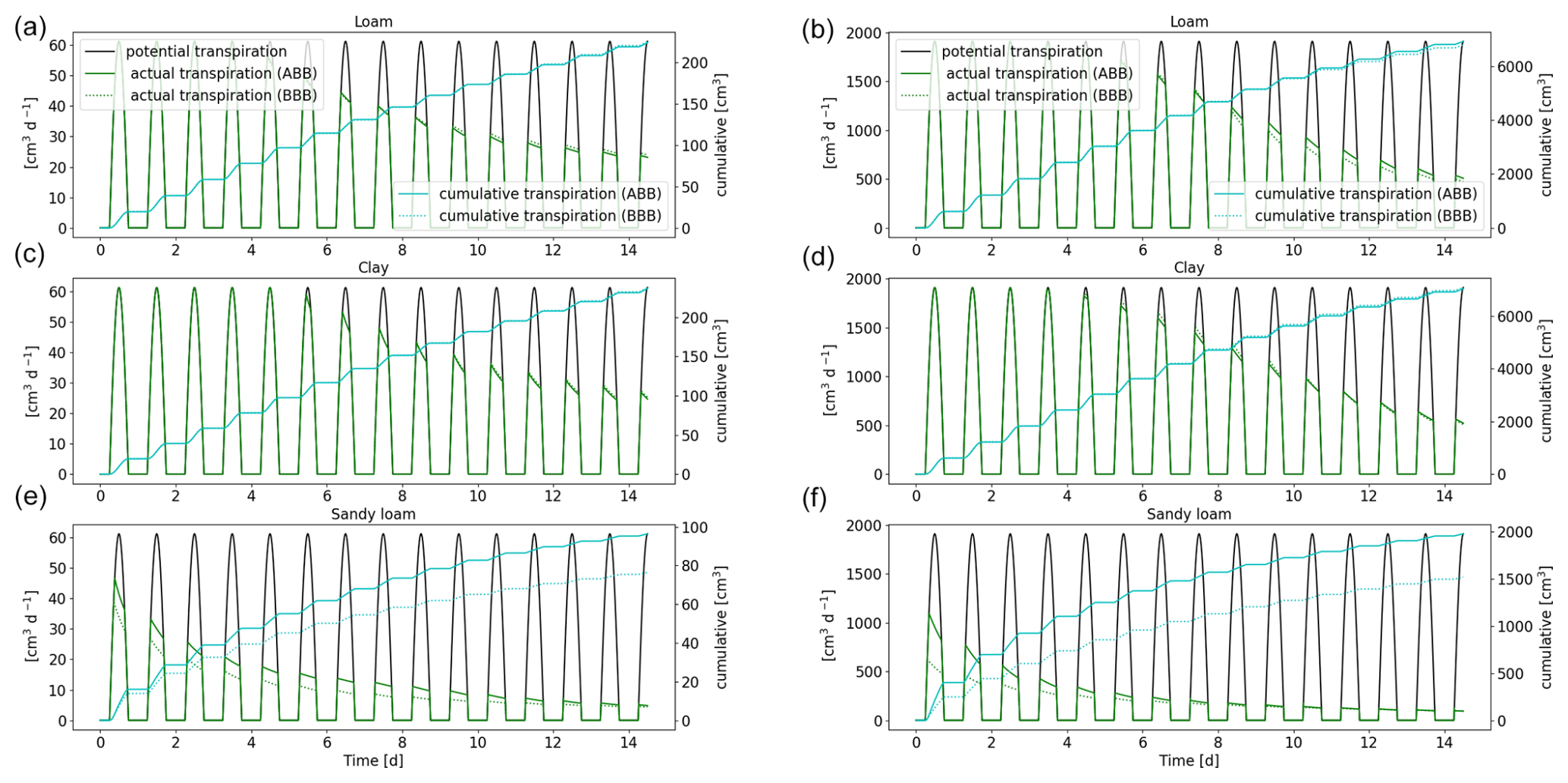
Figure 14 Comparison of the full hydraulic model (ABB) to the aggregated model (BBB) using a 1D soil grid. Potential and actual transpiration of spring barley (a, c, e) and maize (b, d, f) for the soil types loam (a, b), clay (c, d), and sandy loam (e, f). The blue line indicates the cumulative plant water uptake.

3.3.3 Full hydraulic model (ABB) compared to the upscaled root hydraulic model (BBB)

In the next step, we replace the full 3D hydraulic model with a 1D grid (ABB) by the aggregated model (BBB) (see Sect. 2.5) and compare plant actual and cumulative transpiration; see Fig. 14. The approximation works very well for loam and clay: for spring barley, the error is less than 0.8 %; for maize, it is less 1.9 % for loam and 5.7 % for clay after 2 weeks. For sandy loam, the cumulative transpiration is underestimated by around 20 % for spring barley and 9.5 % for maize. This indicates that, in the case of sandy loam, the variation in root xylem potential across one soil layer is high; therefore, we introduce a larger error by using the same total potential at the root–soil interface and the same xylem for each layer; see Eq. (34).

The RWU profiles for spring barley and maize reveal that aggregation works well for loam and clay. However, for sandy soil, the profiles show qualitative differences, strongly underestimating RWU in the lower soil layers for both plants and, in the case of maize, initially overestimating RWU in the upper layers. RWU profiles are presented in Figs. S3 and S4.

Compared to the full 3D root hydraulic model using a 1D soil grid (ABB), computation time was 6–8 times faster for spring barley and 75–100 times faster for the maize using the aggregated model. Generally, the speed-up of the method is mainly dependent on the number root of segments, which is reduced to the number of soil elements. The total speed-up in the aggregated model in a 1D soil (BBB) compared to the full hydraulic model using a 3D soil grid (ABA) is around 25 times for spring barley and 1000 times for maize.

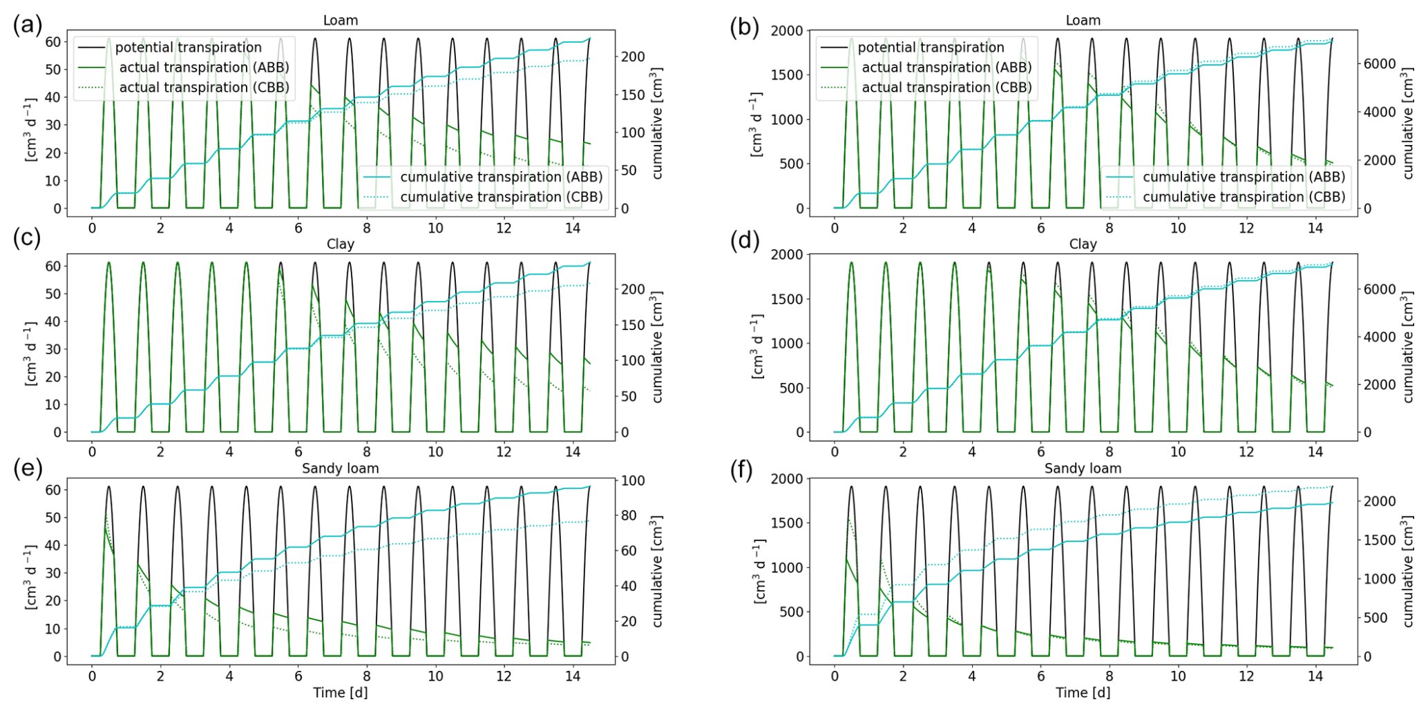
Figure 15 Comparison of the full hydraulic model (ABB) and the parallel root model (CBB) using a 1D soil grid. Potential and actual transpiration of spring barley is shown in panels (a), (c), and (e), and that of maize is shown in panels (b), (d), and (f). The blue line indicates the cumulative plant water uptake.

3.3.4 Full hydraulic model (ABB) compared to the parallel root system (CBB)

As a further simplification, we replace the 3D full hydraulic root model using a 1D grid (ABB) by the parallel root model (CBB) (see Sect. 2.6). Figure 15 shows the actual and cumulative transpiration of spring barley and maize. For spring barley, the parallel root system underestimates the actual transpiration. After 2 weeks, the error of the cumulative transpiration is 11.9 % for loam, 12.3 % for clay, and 20.2 % for sandy loam. For the maize root system, the actual transpiration is overestimated, with errors of 1.7 %, 6.4 %, and 30.4 % for loam, clay, and sandy loam.

For loam and clay, RWU profiles look similar; for spring barley, redistribution is shifted upwards after day 6. As in the case of the aggregated model, sandy loam has the largest error. RWU profiles for the parallel root system model for spring barley and maize are given in Figs. S5 and S6.

The computational speed-up of the parallel root system model (CBB) compared to the full hydraulic model (ABB) is similar to the speed-up of the aggregated model. The reason for this is that, in both models, the degrees of freedom are proportional to the number of soil layers. Compared to the full root hydraulic model, the computation time was 7–8 times faster for spring barley and 96–126 times faster for maize. The total speed-up of the parallel model in a 1D soil (CBB) compared to the full hydraulic model using a 3D grid (ABA) is around 30 times for spring barley and 1180 times for maize.

The advantage of the parallel root system is that the number of parameters is small compared to the full hydraulic model or the aggregated model. The root system hydraulic properties are solely described by SUF, length l, root surface “surf”, and radial conductivity K_r per soil layer (see Sect. 2.6), which can easily be managed by larger-scale models.

Table 3 Error and speed-up for spring barley after 2 weeks: bold numbers on the lower left denote the absolute error in cumulative plant uptake (mm). The corresponding speed-up is given by the italic numbers on the upper right in multiplicity.

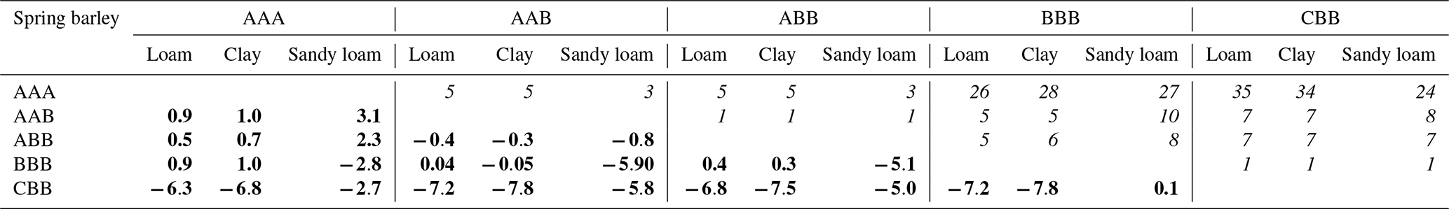
Table 4 Error and speed-up for maize after 2 weeks: bold numbers on the lower left denote the absolute error in cumulative plant uptake (mm). The corresponding speed-up is given by the italic numbers on the upper right in multiplicity.

4 Discussion

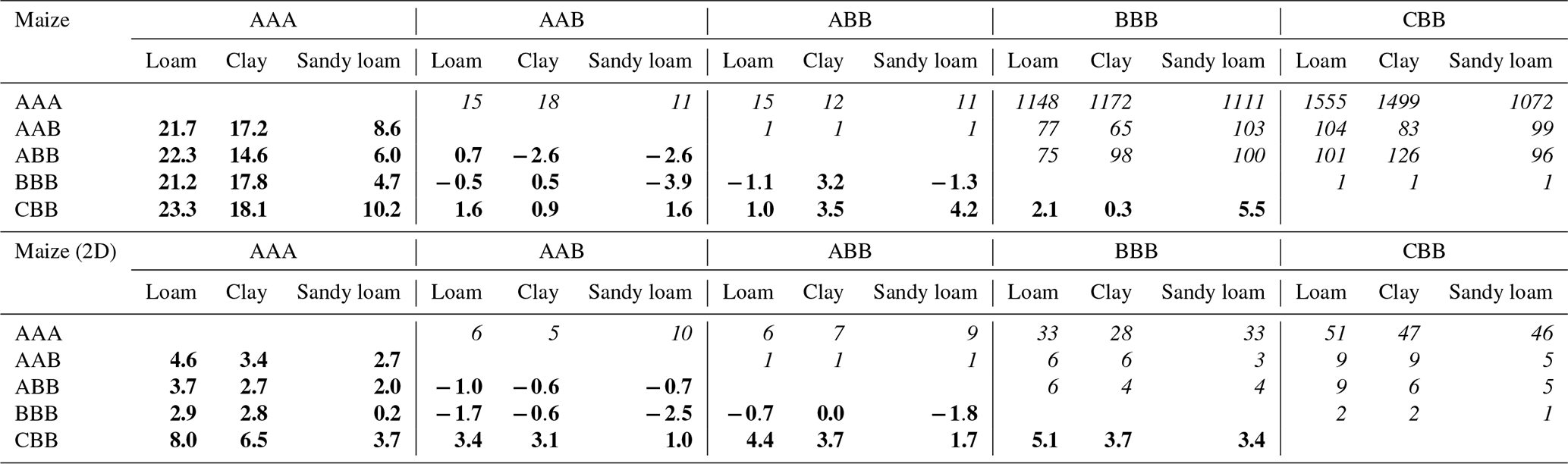
The right spatial and temporal scale of a mathematical model is often a balance between accuracy and efficiency. Equally importantly, small-scale mechanistic models are often hard to parameterize and are not feasible for larger-scale applications (Roose and Schnepf, 2008). In this study, we showed step by step how to develop larger-scale models, from fully parameterized mechanistic hydraulic root–soil interaction models, such as those presented by Schnepf et al. (2023, 2020). We analyse the increase in efficiency by each upscaling step, the error that is introduced, and the number of model parameters that are needed. Tables 3 and 4 show the errors and the corresponding speed-ups introduced by the upscaled models for spring barley and by using a 1D grid or 2D grid for maize. Results suggest that the error introduced by the upscaling steps depends on both the root architecture and the root and soil hydraulic properties. The root hydraulic architectures in our simulations were in range with values for maize (Meunier et al., 2019) and cereals (Baca Cabrera et al., 2024).

Reducing the dimensionality of the macroscopic soil model from 3D to 1D (AAA vs. AAB) works well if lateral water movement can indeed be neglected. This is the case if roots are evenly distributed with similar root hydraulic properties (Couvreur et al., 2014). Furthermore, even if the roots are evenly distributed, they also need to be sufficiently dense, depending on the soil hydraulic conductivity. Otherwise, isolated depletion zones can develop, which would lead to horizontal fluxes in the 3D soil domain that are not represented in the 1D soil layer. For spring barley, this worked well for loam and clay, but, for sandy loam, we observed a larger error due to low soil conductivity. For maize, errors were larger due to its non-uniform root distribution. Generally, the accuracy of 1D soil models is dependent on the inter-row and planting distance. In the maize scenario, root density strongly varies in the direction between two plant rows. Therefore, to maintain a more precise model, it is recommended to neglect only one dimension, keeping the direction orthogonal to the planting row and averaging along the direction of the planting row, where changes in root density are expected to be smaller. In the case of maize, using a 2D macroscopic soil model reduced the error, with a speed-up between 5 and 10 times dependent on the soil type (see Table 4).

We used a new method to determine the outer radii of the perirhizal zones based on Voronoi diagrams in 3D, similarly to what Kohl et al. (2007) did for 2D root observations in trenches. We compared these more exact results to the common approach calculating the radii based on length, surface, or volume densities (AAB vs. ABB), e.g. Schröder et al. (2008), Van Lier et al. (2006). Generally, the approximation using densities works very well, with a negligible impact for 3D soil grids and a stronger impact using 1D soil layers. In the 1D case, using the Voronoi approach leads to higher radii at the root tips, since the Voronoi cell volumes are statistically larger at the root tip nodes, where a small root segment has access to a large soil volume. Thus, those parts of the root system with a higher root radial conductance have access to a larger soil volume compared to the uniformly distributed roots, leading to an increased actual transpiration. Since restricting the model to vertical movement leads to an overestimation of actual transpiration, the underestimation of actual transpiration of the more classical approaches seems beneficial. Overall, we showed that perirhizal radii based on length, surface, and volume densities introduced only a small error compared to the other upscaling steps. For both plants, the sandy loam scenario led to the highest discrepancies in cumulative plant uptake because low soil conductivity leads to steeper gradients in the rhizosphere and generally increases the importance of the perirhizal zones.

Upscaling by aggregating RWU from root segment to soil element level was introduced by Couvreur et al. (2012), not considering any perirhizal conductance. In this case, the total potential at the soil–root interface is the same for all root segments in each soil layer in the full hydraulic model and in the aggregated one. Vanderborght et al. (2023) included perirhizal conductance, which leads to individual total potentials at the soil–root interface for the full hydraulic model, and aggregation leads to the additional assumption that these total potentials at the soil–root interface are equal in each soil layer. In this study, we tested this assumption for the first time in dynamic settings. The approximation performs well in loam and clay soil because of the higher soil conductivity, with relative errors less than 1 % for spring barley (0.04 and 0.05 mm absolute error) and maize (±0.5 mm absolute error for 1D; −1.7 and −0.6 mm for 2D) compared to reference scenario AAB. For sandy loam, cumulative transpiration was underestimated by around 23 % for both plants (5.9 mm for spring barley; −3.9 mm for maize 1D and −2.5 maize 2D); see Tables 3 and 4. The speed-up of the method is dependent on the number of segments within the root system. Depending on soil type, the aggregated model is at least 26 times faster for spring barley and 1111 times faster for maize using a 1D grid and 28 times faster for maize using a 2D grid.

In a further step, we replaced the root architecture model with a parallel root model to obtain a more efficient model with fewer parameters, which is easier to parameterize and can be used in an easier way by larger-scale models (Vanderborght et al., 2024). It relies only on the root system conductivity K_rs and values given per soil layer (SUF, length l, root surface “surf”, and radial conductivity K_r) and needs no additional information on root system topology. Results are exact when the soil–root interface potentials are uniform. For non-uniform soil–root interface potentials, the uptake compensation is not exact anymore. Under the dynamic depletion scenarios, this approach led to an underestimation of cumulative uptake for spring barley and an overestimation for maize, owing to different root hydraulic properties. The parallel model (CBB) is an efficient approximation, with the largest speed-ups where the lumped parameters are derived from the mechanistic parameters of the detailed model (AAA).

Within the perirhizal zone, the steep gradients in water potential towards the roots are described using the steady rate approach of Schröder et al. (2008). We emphasize that this analysis of upscaling methods could be done with more complex rhizosphere models. The water potential near the root surface depends on a variety of biochemical processes leading to complex mechanistic models that are often hard to parameterize. Important rhizosphere processes affecting root water uptake include mucilage (Schwartz et al., 2016), root hairs (Duddek et al., 2023), mycorhizal fungi (Püschel et al., 2020), and the osmotic potential (Wang et al., 2023). They are often not explicitly described by the model, but they enter the model as effective or lumped parameters. Furthermore, one could aim to reduce the errors introduced by the dimensionality reduction, especially in row crops, e.g. by numerical homogenization. In general, to obtain effective models and parameters, a homogenization procedure can be a valuable tool in model development (Hornung, 1996).

5 Conclusions

RWU is crucial for soil water balance and plant development. We describe soil–root hydraulics and dynamic root architecture in a mechanistic way and analyse upscaling methods to develop efficient sink terms for land surface or crop models. In this study, we explored the mathematical fundamentals of the different upscaling approaches and the impact of each simplification step. Reducing the dimensionality of the macroscopic soil model from 3D to 1D (AAA vs. AAB) worked well if lateral water movement can indeed be neglected. This depended on root distribution and on root and soil hydraulic properties. Assuming homogeneously distributed roots to calculate the outer perirhizal radii provided accurate results regarding RWU (AAB vs. ABB) but needs review for more complex rhizosphere models. Generally, the approximation had a stronger impact using coarse 1D soil layers, which leads to an underestimation of the actual transpiration. The exactly upscaled model (BBB) with uniform soil–root interface water potential offered a large speed-up in computation time, introducing only small errors compared to the error introduced by dimensionality reduction. The parallel root model (CBB) introduced slightly larger errors but can be implemented more easily in larger-scale models due to a lower number of model parameters.

This study highlights the importance of carefully considering the trade-offs between model complexity and accuracy. By pinpointing the sources of errors and understanding where they accumulate or cancel out, we provide guidance for choosing appropriate models based on the required performance and accuracy. This knowledge facilitates the development of new sink terms and enhances the reliability of RWU modelling in diverse agricultural and environmental contexts.