Scale dependency in modeling nivo-glacial hydrological systems: the case of the Arolla basin, Switzerland

Hydrological modeling in alpine catchments poses unique challenges due to the complex interplay of meteorological, topographical, geological, and glaciological drivers with streamflow generation. A significant issue arises from the limited availability of streamflow data due to the scarcity of high-elevation gauging stations. Consequently, there is a pressing need to assess whether streamflow models that are calibrated with moderate-elevation streamflow data can be effectively transferred to higher-elevation catchments, notwithstanding differences in the relative importance of different streamflow-generation processes. Here, we investigate the spatial transferability of calibrated temperature-index melt model parameters within a semi-lumped modeling framework. We focus on evaluating the melt model transferability from the main catchment to nested and neighboring subcatchments in the Arolla valley, southwestern Swiss Alps. We use the Hydrobricks modeling framework to simulate streamflow, implementing three variants of a temperature-index snow and ice melt model (the classical degree-day model, the aspect-related model, and the Hock temperature-index model). Through an analysis of streamflow simulations, benchmark metrics consisting of resampled and bootstrapped discharge time series, and model performance metrics, we demonstrate that robust parameter transferability and accurate streamflow simulation are possible across diverse spatial scales. This finding is conditional upon the melt model applied, with melt models using more spatial information leading to convergence of the model parameters until we observe overparameterization. We conclude that simple semi-lumped models can be used to extend hydrological simulations to ungauged catchments in alpine regions and improve high-elevation water resource management and planning efforts, especially in the context of climate change.

1 Introduction

Understanding the driving factors of nivo-glacial streamflow regimes is essential for managing high alpine catchments and their water resources under global change. With ongoing warming, the long-, intermediate-, and short-term storage capacities of alpine nivo-glacial systems (e.g., storage capacities of subglacial drainage network, snow cover, glacier ice) will be impacted (Jansson et al., 2003; Huss et al., 2008), and high alpine catchments may transition from nivo-glacial streamflow regimes to dominantly nival regimes (Horton et al., 2006). Currently, alpine glaciated catchments and downstream areas receive a strong surplus of meltwater from snow during spring and early summer (Penna et al., 2017; Engel et al., 2019; Zuecco et al., 2019), gradually switching to glacier meltwater towards the end of summer. The timing and amount of snowmelt and glacier melt are strongly impacted by global warming and related glacier retreat, leading to changes in streamflow regimes (e.g., Singh and Kumar, 1997; Bradley et al., 2006). These changes in streamflow regimes and runoff generation characteristics have important consequences in terms of sediment transport, hydropower production (Gabbud et al., 2016), flood prediction, and ecology (Tague et al., 2020).

Despite this, high alpine catchments often lack discharge monitoring stations due to their sparse population and difficulty of access. In highly glacierized catchments (i.e., glacial cover >50 %), there are very few gauging stations that provide reliable and long-term streamflow records. This makes attributing historical changes in streamflow regimes to glacial sources challenging and inevitably requires recourse to modeling, not just to predict the future but also to understand the past.

Hydrological models are commonly classified into distributed, semi-distributed, semi-lumped, and lumped models (Horton et al., 2022). Distributed models compute the storage and mobilization of water at a grid-cell scale, with parameters that vary in space (fully distributed) or are partially kept constant (semi-distributed). Semi-lumped models define areas of interest based on relevant physical parameters (e.g., elevation, aspect, stream network topology), and lumped models consider the catchment to be a single unit. While (semi-)distributed and semi-lumped models allow some spatial variations to be taken into account and provide a more detailed representation of the processes, lumped models have to represent the functioning of the entire system. The advantage and popularity of (semi-)lumped models should not be attributed solely to their computational efficiency, which facilitates multiple model simulations. They also represent an optimal level of model complexity with respect to available input and output data from a downward model development perspective (Sivapalan et al., 2003); they furthermore operate at a scale at which averaging of small-scale processes enables a reliable representation of dominant hydrological processes (Clark et al., 2016).

However, one of the main drawbacks of (semi-)lumped models is that streamflow can only be modeled reliably at the selected control points (outlets) for which the model parameters have been calibrated against observed streamflow. Simulated streamflow at other locations within or near the catchment might not reliably represent the actual system dynamics. In other words, the calibrated parameters might not be transferable to other locations of the stream network (subcatchments) within the system. This transferability issue is particularly important in high alpine catchments for snow and ice melt parameters, as meltwater plays a major role in streamflow generation processes. The proportion of streamflow that is melt-derived (either from snow or ice) and the dominant drivers of melt (i.e., components of the energy balance) will change as the basin outlet selected for simulation is shifted upstream or downstream, which means that melt parameters need to be scale-independent. This difficulty is exacerbated in catchments with strong topographic gradients and spatial heterogeneity, where the complex spatial averaging complicates the extraction of melt-driven streamflow simulations at smaller scales, which is typically the case in glaciated catchments. One possible solution to increase the spatial transferability of calibrated models is the use of additional observed data to better constrain model parameters (Efstratiadis and Koutsoyiannis, 2010) and thereby to increase their reliability, in particular in view of input data uncertainty (van Tiel et al., 2020) and in view of simulating change conditions (climate change, land use change). In the field of high alpine streamflow simulation, the focus is on the value of glacier mass balance or snow data to ensure that the calibrated streamflow is right for the right reasons (Kirchner, 2006) rather than due to compensating effects (see the review by van Tiel et al., 2020). Examples include the work of Parajka and Blöschl (2008), Şorman et al. (2009), Koboltschnig et al. (2008), Immerzeel et al. (2009), Konz and Seibert (2010), Griessinger et al. (2016), Gyawali and Bárdossy (2022), Tiwari et al. (2024), and Ruelland (2024), which all focus on different aspects of parameter reliability as a function of model calibration strategy. For example, the work of Griessinger et al. (2016) underlines the fact that the incorporation of snow data is especially important for high-elevation catchments and snow-rich years. However, this wealth of literature does not address the question of how to transfer calibrated parameters to other catchments or to subcatchments, which is the focus of hydrological parameter regionalization methods.

Parameter regionalization techniques (Guo et al., 2021) in hydrological modeling have been developed to facilitate the transfer of model parameters from gauged to ungauged locations (e.g., Mosley, 1981; Abdulla and Lettenmaier, 1997; Bardossy and Singh, 2008). Regionalization methods can be divided into two categories (Samaniego et al., 2010): post-regionalization and simultaneous regionalization. Post-regionalization methods calibrate a model in several basins independently and then statistically link the calibrated model parameters to basin predictors (e.g., mean catchment elevation, stream network density, geology, areal proportion of porous aquifers) using a transfer function (e.g., Abdulla and Lettenmaier, 1997; Seibert, 1999; Parajka et al., 2005; Wagener and Wheater, 2006). Simultaneous regionalizations aim to calibrate model parameters for several basins while taking into account transfer functions that link model parameters to catchment characteristics (e.g., Hundecha and Bárdossy, 2004; Götzinger and Bárdossy, 2007; Fernandez et al., 2000; Troy et al., 2008). The second category of methods was developed to add additional spatial constraints to parameter calibration and to avoid artifacts of the optimization algorithm. In all these methods, the need to define a function that links catchment characteristics and model parameters is subject to additional uncertainties, and snow parameters are often kept constant in such approaches (Götzinger and Bárdossy, 2007; Kling and Gupta, 2009).

Overall, the number of parameter regionalization studies in alpine areas remains small (Horton et al., 2022), and the spatial transfer of melt model parameters is still a crucial topic for the prediction of streamflow in catchments without observed streamflow (Guo et al., 2021).

Spatial parameter transfer is particularly challenging in data-sparse high-elevation catchments where glacier melt, interannual snow storage, and highly uncertain precipitation and evapotranspiration can lead to considerable parameterization difficulties (Schaefli and Huss, 2011). A particular challenge in such catchments is the estimation of snowmelt and glacier melt contributions, which, for practical data reasons, is often limited to the use of temperature-index melt models (TI) that link melt rates to air temperature (Eq. 1, Rango and Martinec, 1995):

$$\begin{array}{}\text{(1)}& M_{\mathrm{TI}}\left(t\right)=\left\{\begin{array}{ll}{a}_j\left(T_{\mathrm{a}}\right(t)-T_{\mathrm{T}})& :T_{\mathrm{a}}\left(t\right)>T_{\mathrm{T}}\mathrm{with}j\in \mathrm{snow},\mathrm{ice}\\ \mathrm{0}& :T_{\mathrm{a}}\left(t\right)\le T_{\mathrm{T}},\end{array}\right.\end{array}$$

where M_TI(t) is the melt rate at time step t (mm d⁻¹), a_j is the degree-day factor for ice or snow (mm d⁻¹ °C⁻¹), T_a is the air temperature, and T_T is the threshold melt temperature.

Although it is commonly admitted that TI models present a good option for extrapolation to larger scales because of the persistency of temperature over large areas (Frenierre and Mark, 2014), the spatial transferability of the related parameters calibrated at the outlet of a catchment to the outlet of a neighboring catchment exhibiting different characteristics (elevation, aspect, glacial cover) can be questioned (Gabbi et al., 2014; Samaniego et al., 2010) and has rarely been investigated. This challenge was exemplified for nested catchments by Comola et al. (2015), who studied the influence aspect and found significant variability in the calibrated degree-day factors for small catchments (<7 km²) when using a simple temperature-index model.

One option to regionalize melt model parameters is to compute them directly based on in situ snow observations, which was already presented by Martinec (1960) (for an application to streamflow modeling see the work of Hingray et al., 2010). Similarly, they can be computed from remotely sensed snow extents: the work of He et al. (2014) shows that such spatially variable melt model parameters can improve streamflow simulations compared to spatially constant parameters. Such approaches are rare because the value of temperature-index melt models is inherently linked to streamflow simulation and most studies therefore calibrate melt parameters against streamflow.

In this study, we investigate the transferability of the melt and streamflow calibrated parameters between subcatchments and neighboring catchments considering different melt models and with respect to very high-quality discharge measurements obtained from a hydropower company (see Sect. 2.2 and Fig. S14). In view of this exceptional discharge dataset, we chose not to use remotely sensed snow data because the preprocessing of remotely sensed snow extents and their use for model calibration include uncertainty (Parajka and Blöschl, 2006, 2008), which would obscure our analysis.

For our analysis, we calibrate our model for seven catchments, then take the parameters of the largest catchment and transfer them to its three nested watersheds and three other neighboring catchments. We then analyze the loss of accuracy related to the transfer of parameters. To ensure that our conclusions hold for different commonly used objective functions and assess the sensitivity to these objective functions, we use two different metrics: the Nash–Sutcliffe (NSE; Nash and Sutcliffe, 1970) and Kling–Gupta efficiency (KGE; Gupta et al., 2009). These two very common metrics do not translate into one another: the NSE measures the error variance related to the variance of the discharge, while the KGE measures correlation, variability bias, and mean bias. NSE and KGE are differently sensitive to discharge errors: for example, for high-variation regimes that show small errors and large bias, the NSE would give a very promising value, while the KGE would not (Knoben et al., 2019). We carry out this transferability assessment with three temperature-index melt models of increasing complexity and try answering the question: could incorporating additional spatial information into more complex TI models increase their spatial transferability?

2 Study area: the upper Arolla river basin and its subcatchments

2.1 Presentation of the study area

We use data (Table 3) from the Arolla river basin located in the southwestern Swiss Alps (Fig. 1). A local hydropower company provided 15 min resolution streamflow recordings of very high quality given strict regulatory requirements for monitoring water use (Lane and Nienow, 2019). The Bertol Inférieur (BI) gauging station is fed by water draining from four subcatchments (Table 1): Bertol Supérieur (BS), Haut Glacier d'Arolla (HGDA), Mont Collon (MC), and Vuibé (VU). The BI catchment, with an area of 26.0 km², provides a good opportunity to test the transferability of hydrological parameters to nested catchments as there are three subcatchments that are also gauged upstream: BS (2.6 km² area), HGDA (13.2 km²), and VU (2.2 km²). Remaining drainage to BI comes from the MC catchment or from points located between the BS, HGDA, and VU gauges and the BI gauge (Fig. 1). Immediately to the north of the VU catchment is the Pièce catchment (PI), draining an area of 2.9 km², and the Tsijiore Nouve (TN) catchment with a drainage area of 4.8 km². On the other side of the valley, immediately to the north of the BS catchment, is the Douves Blanches (DB) catchment with a drainage area of 1.5 km². These catchments allow us to test the transferability of hydrological parameters to neighboring catchments. The elevation of these basins ranges from 2112 m a.s.l. (the elevation of the BI gauging station) to 3838 m a.s.l. (the Grand Bouquetins peak, located in the Haut Glacier d'Arolla). At these elevations, it is extremely unusual to have such high-quality streamflow data for small, highly glacier-covered catchments.

Table 1 Catchments used in the simulations and their properties.

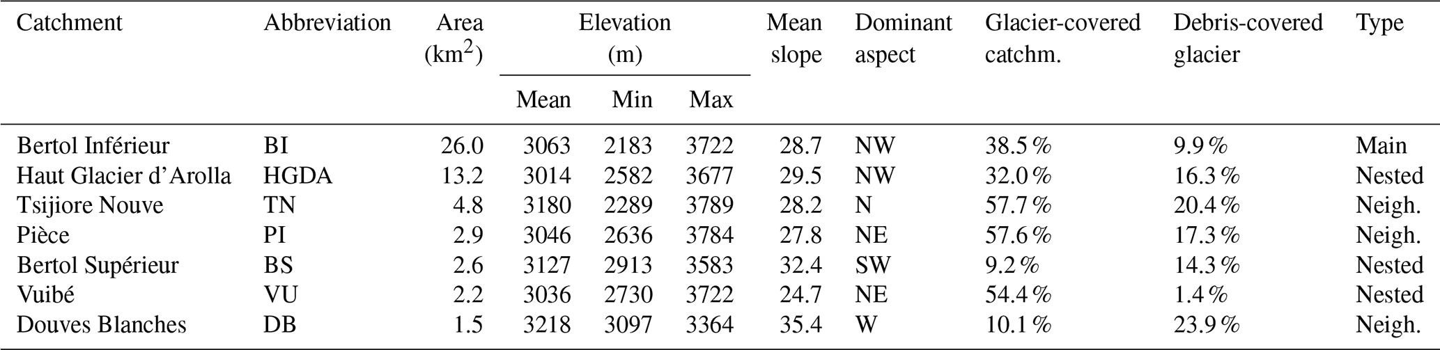
The upper Arolla river basin presents a variety of aspects (Fig. 1b), and its subcatchments have different general orientations (Fig. 1c). The glacial cover within the Arolla basin decreased (Fig. 1d) from 66.5 % in 1850 to 38.5 % in 2016 for the BI catchment (GLAMOS, 2020), while remaining relatively constant since 2009. The geology of the study area consists mainly of metamorphic and igneous rocks, extensively covered with till and colluvial deposits (SwissTopo, 2025b, Fig. S3). The geomorphological characteristics of the subcatchments are generally similar. DB, BS, TN, and the northern part of HGDA all feature some rock glaciers (Lambiel et al., 2016), although their relative area is more significant for DB and BS.

Numerous studies have been carried out in the upper Arolla basin over the years on topics ranging from glacier dynamics to subglacial hydrology and sediment transport to hydrology (Sharp et al., 1993; Brock et al., 2000; Mair et al., 2002, 2003; Swift et al., 2002, 2005; Arnold, 2005; Pellicciotti et al., 2005; Dadic et al., 2010; Gabbud et al., 2015, 2016; Lane and Nienow, 2019), which makes this study area optimal for a technical study on hydrological parameter transferability.

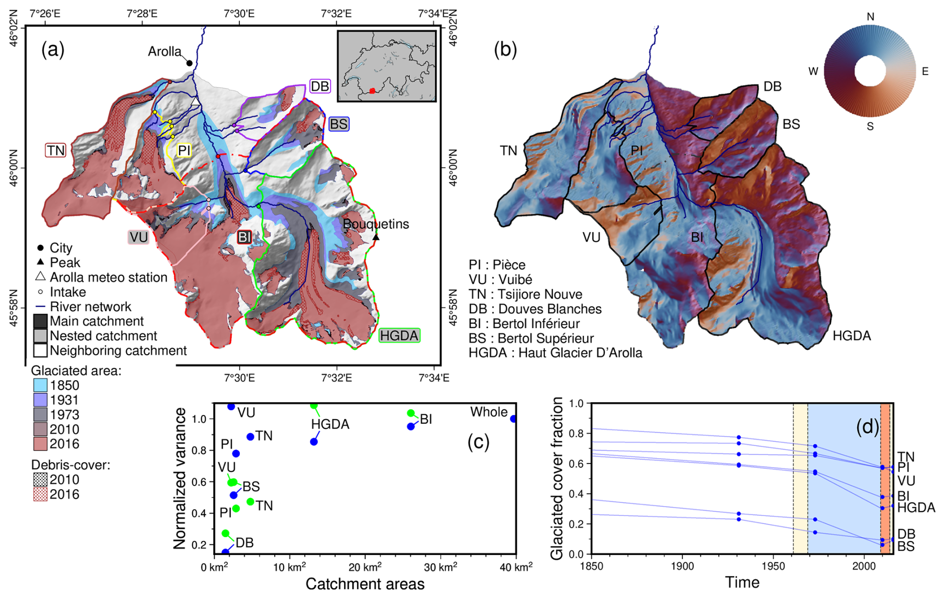
Figure 1 (a) Overview of the modeled catchments and subcatchments in the upper part of the Heremence valley, in the Arolla catchment. Changes in glacial cover through time are indicated in shades of blue and red. The inset map shows the location of the study catchments in the Swiss Alps. (b) Aspect of the study area. (c) Aspect variogram derived from the aspect variance of each glacier (in blue) and each catchment (in green), normalized by the variance in the total glaciated area and total catchment (whole), as done by Comola et al. (2015). (d) Glacial cover fraction through time, with the study period highlighted in orange and the available discharge period and meteorological data in blue and yellow, respectively. Topography is obtained from the SwissTopo DHM25 dataset (SwissTopo, 2025a) and glacier extents are from the GLAMOS inventory (GLAMOS, 2020, Table 3).

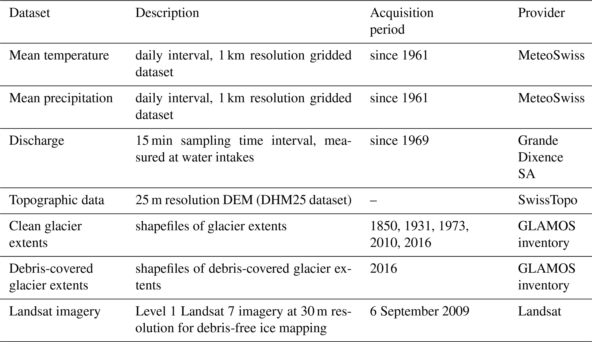
2.2 Hydrometeorological datasets

We use MeteoSwiss datasets for daily mean precipitation (MeteoSwiss, 2019a) and daily mean temperature available at 1 km resolution for Switzerland (MeteoSwiss, 2019b).

Discharge data were provided by Grande Dixence SA (personal communication, 2024) at seven water intakes. In Switzerland, regulatory standards require hydroelectric power production companies to report water abstraction details to the authorities. In the upper Arolla river basin, discharge data have thus been provided at a 15 min resolution since 1969. Each basin features a calibrated water level recorder, initially utilizing a chart recorder and later upgraded to a pressure transducer with digital data logging. Water levels are measured across a broad-crested weir, ensuring highly reliable discharge records (±0.01 m³ s⁻¹ for regulatory compliance). Under very high flow conditions, the intake overflows and only some of the water is recorded. However, since any loss of water is a financial loss, the intake has been designed to capture practically all the discharge. Such overflows are therefore possible but infrequent. Furthermore, the current ecological minimum flow was only introduced in one of the intakes, BI, as of 2018, after the period used in this study (Tobias et al., 2023). The intakes defining the extent of each subcatchment are sometimes multiple, as with DB and VU, which both present two intakes, and PI, which presents four (See Fig. 1). Thus, the discharge is the sum of the corresponding intakes.

With the exception of BI, discharge data were already preprocessed by Lane and Nienow (2019) to eliminate drawdown events linked to sediment removal during intake flushing. Since these drawdown periods typically last between 30 and 60 min, they can be visually recognized using the method outlined in the work of Lane et al. (2017). After the removal of data portions corresponding to such drawdowns, any missing data points were linearly interpolated. However, for the VU intake, data were unavailable from 31 August to 31 December 2011 due to intake maintenance work. In our study, we excluded this last period for VU and applied the same preprocessing method to the BI discharge time series, removing drawdown events and discarding associated time periods (in blue, Fig. 2). Furthermore, the water from the HGDA, BS, and VU intakes is diverted and does not pass through the BI intake. We thus added the records of its upstream nested intakes to the BI discharge record (the actual measurements in BI is called BIrest; see Fig. 2). We propagated to BI the intake maintenance work of VU and the drawdown removals of BIrest by discarding the affected time periods. The time taken by the water to reach the BI intake from the upstream intakes is approximately 15–30 min depending on the day, which is negligible at the daily scale (Fig. S13). Subsequently, the 15 min time step discharge datasets were summed up to daily time step datasets after the preprocessing.

Due to the confidentiality of the original discharge data, these datasets are shown here normalized by the same highest observed discharge values for all catchments (see Figs. 2, 4, 6, 8, 9, 11, and 14). The normalized dataset is called “normalized discharge” when the discharge was expressed in m³ s⁻¹ and “specific normalized discharge” when the discharge was expressed in millimeters.

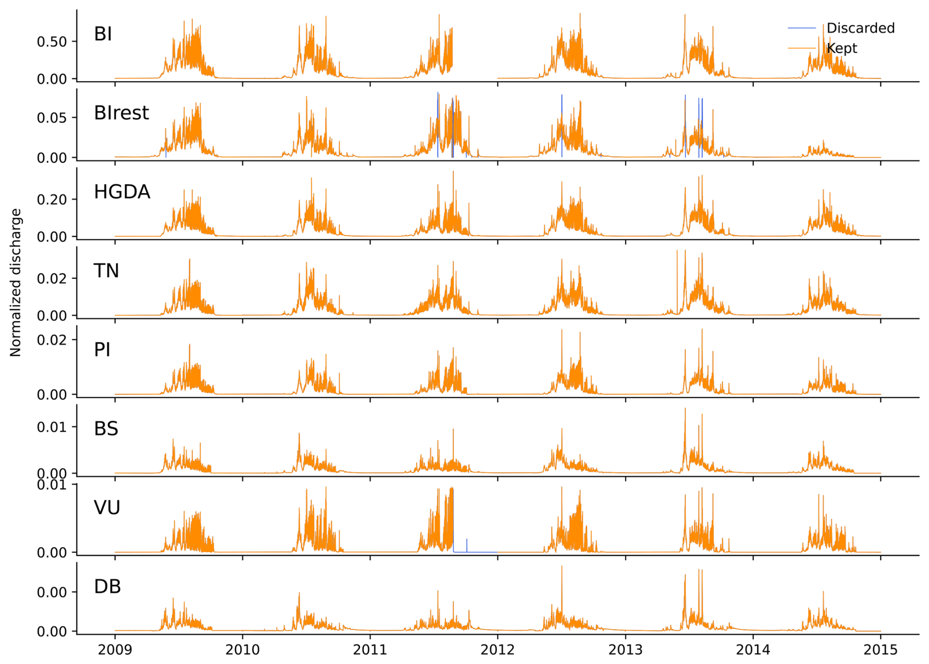
Figure 2 Observed discharge series for all subcatchments: Comparison of the discharge series kept for calibration in Hydrobricks (orange) with the discarded periods (blue). Discharge (unit: m³ s⁻¹) is normalized by the same highest observed discharge values for all catchments. The BI discharge corresponds to BIrest + HGDA + BS +  VU.

Glacier extents for the years 2010 and 2016 were obtained from the GLAMOS inventory (Fig. 1; GLAMOS, 2020; Linsbauer et al., 2021; Fischer et al., 2014). This inventory specifies the debris cover extent for the year 2016. To obtain older debris cover trends, we used the algorithm developed by Shokory and Lane (2023), now available in an ArcGIS Pro toolbox, and computed the 2010 extents based on Landsat Level 1 imagery (for details, see Sect. S4). We assumed the glacial cover of 2009 to be identical to 2010.

We derived the topography from the SwissTopo DHM25 dataset (SwissTopo, 2025a) available at 25 m resolution. From this topography, we automatically extracted the catchment areas, except for VU. VU requires manual correction of its southern extent due to the presence of thick ice cover, which complicated the identification of the drainage divide (Fig. 6 of Bezinge et al., 1989; Hurni, 2021).

3 Methods

3.1 Hydrological modeling with Hydrobricks

Hydrobricks (v0.7.2; Horton and Argentin, 2024) is a hydrological modeling framework that implements the semi-lumped GSM-SOCONT model (Glacier and SnowMelt – SOil CONTribution; Schaefli et al., 2005) to simulate nivo-glacial hydrological regimes. The model consists of two main components: (a) the reservoir-based SOCONT model, which incorporates a linear reservoir method to account for slow storage contribution (emulation of subsurface ground water) and a nonlinear reservoir approach to address quick runoff, and (b) the GSM model, which is specifically designed for glacier-covered catchments. The Hydrobricks framework is based on a C++ core integrated into a Python interface, which allows for enhanced computing performances.

The model discretizes the catchment into hydrological response units (HRUs) by elevation, aspect, and potential clear-sky direct solar radiation. The HRUs can have fractional land cover types, here “glacier” for glacier-covered areas and “ground” for non-glacier-covered areas. The distinction between debris-covered glacier areas (“glacier_debris”) and debris-free glacier areas (“glacier_ice”) can also be made (Shokory and Lane, 2023). The processes occurring within the same land cover type but in different HRUs are assigned identical parameters.

Following GSM-SOCONT's original structure, the model behavior differs between the glacier-covered area and the ice-free part. For the ice-free fractional part of a given HRU, surface and subsurface runoff components, along with baseflow from melt and rainfall (Fig. S1), are computed per HRU and summed across all HRUs to build the non-glacier streamflow component at the outlet. For glacier-covered areas, the liquid water from melt and rainfall produced by each HRU is fed into two lumped parallel linear reservoirs shared by all HRUs. The purpose of these reservoirs, which only apply to glacier surfaces, is to represent the glacier's retention effect on water flow. For a detailed workflow, refer to Fig. S1 and Schaefli et al. (2005).

The transition from rainfall to snowfall is defined in a fuzzy approach (Schaefli and Huss, 2011) between 0 °C for the lower end (T_s-r, min) and 2 °C for the upper end (T_s-r, max). Snow and ice start melting at a threshold melt temperature T_T defined at 0 °C, and ice can only melt when it is no longer covered by snow.

We use the SPOTPY library (Houska et al., 2015) provided with Hydrobricks for parameter optimization with the Shuffled Complex Evolution algorithm of the University of Arizona (SCE-UA). The SCE-UA algorithm is designed to prevent remaining stuck in local optima. We use it in combination with the Nash–Sutcliffe (NSE; Nash and Sutcliffe, 1970) and Kling–Gupta efficiency (KGE; Gupta et al., 2009) performance criteria to find the best combination of parameters (Table 2) after 10 000 simulations.

3.2 Hydrobricks developments

In the original version of GSM-SOCONT (Schaefli et al., 2005), precipitation type (snow or rain) is determined by a temperature threshold and melt is calculated through a classic TI melt model. Two new melt models were implemented in Hydrobricks: the aspect temperature-index model (ATI) and the temperature-index model of Hock (HTI).

The aspect temperature-index model (ATI) is based on the discretization of the study area by aspect (north, south, and east/west) and the use of a distinct degree-day factor depending on aspect. A more complex model, the temperature-index melt model of Hock (HTI; Hock, 1999), links potential clear-sky direct solar radiation to melt rates (Eq. 2):

$$\begin{array}{}\text{(2)}& M_{\mathrm{HTI}}\left(t\right)=\left\{\begin{array}{ll}(m+r_j{I}_{\mathrm{pot}})\left(T_{\mathrm{a}}\right(t)-T_{\mathrm{T}})& :T_{\mathrm{a}}\left(t\right)>T_{\mathrm{T}}\\ & \mathrm{with}j\in \mathrm{snow},\mathrm{ice}\\ \mathrm{0}& :T_{\mathrm{a}}\left(t\right)\le T_{\mathrm{T}},\end{array}\right.\end{array}$$

where M_HTI is the melt rate (mm d⁻¹), m is the melt factor common to both ice and snow (mm d⁻¹ °C⁻¹), r_j is the radiation factor for ice or snow (mm d⁻¹ °C⁻¹ m² W⁻¹), I_pot is the potential clear-sky direct solar radiation (W m⁻²), T_a is the air temperature, and T_T is the threshold melt temperature. Thus, while the ATI model represents a first attempt at handling spatial differences in melt rates, the HTI model has the benefit of directly taking into account irradiation, which should make it better suited to reproduce melt rates in catchments influenced by aspect and cast shadows (e.g., Gabbi et al., 2014).

The HTI model requires computation of the potential clear-sky direct solar radiation I_pot, implemented here using the definition of Hock (1999, Eq. 3):

$$\begin{array}{}\text{(3)}& I_{\mathrm{pot}}=I_{\mathrm{0}}{\left({\displaystyle \frac{R_{\mathrm{m}}}{R}}\right)}^{\mathrm{2}}{\mathrm{\Psi }}_{\mathrm{a}}^{\left(\frac{P}{P_{\mathrm{0}}\cos \left(Z\right)}\right)}\cos \left(\mathit{\theta }\right),\end{array}$$

where I₀ is the solar constant (1368 W m⁻² ), ${\left(R_{\mathrm{m}}/R\right)}^{\mathrm{2}}$ is the Earth's orbit's eccentricity correction factor composed of R and R_m the instantaneous and mean Sun–Earth distances, Ψ_a is the mean atmospheric clear-sky transmissivity, P and P₀ are the local and mean sea-level atmospheric pressures, Z is the local zenith angle, and θ is the angle of incidence between the normal to the grid slope and the solar beam. The potential direct solar radiation, computed on a 15 min interval, is set to 0 when a point is not directly irradiated by sunlight (nighttime and cast shading brought by surrounding relief), then summed at the daily scale to obtain the daily potential direct solar radiation I. This 15 min interval allows one to account for changes in the Sun's position as well as its rising and setting times during the year.

For the TI model, based on temperature only, the HRUs are evenly spaced elevation bands (Schaefli et al., 2005). For the ATI and HTI models, the HRUs reflect the elevation variations as well as the aspect or the mean annual irradiation variations. To avoid any HRU scaling influence on parameter transferability (Liang et al., 2004; Troy et al., 2008), we use a spacing of 40 m for elevation, three categories for aspect (north, south, and east/west to group by degree of Sun exposure), and a spacing of 65 W m⁻² for potential direct solar radiation for all catchments (Fig. S2). Furthermore, in contrast to earlier studies employing GSM-SOCONT/Hydrobricks, which relied on monitoring station data to derive meteorological lapse rates across the different elevation bands, we needed to derive our meteorological input from gridded datasets. Our study therefore adopts a distinct methodology, extracting meteorological input for each HRU directly from gridded datasets. This involves quantifying how much the different cells in the gridded datasets contribute to each HRU. We do this by downscaling the grid of the meteorological data (1 km) once to the digital elevation model (DEM) resolution (25 m): we compute the weights representing the contribution of each data cell to each HRU based on their spatial coverage, then use these weights to calculate the mean values for each HRU for each daily time step. This allows direct use of future climate model outputs often provided as gridded datasets. The evapotranspiration is then computed at the HRU level from mean values of temperature, following the Hamon equation (Hamon, 1963).

In the case where we differentiate between debris-covered and debris-free glacier coverage, we also have to adapt the melt models by introducing new melt parameters governing the ice melt. The TI model switches from a single parameter (a_ice) to two parameters (a_deb-free and a_deb-cov). The ATI model goes from three parameters (a_ice, j with j∈ N, S, E–W) to six parameters (a_{deb-free, j} and a_{deb-free, j} with j∈ N, S, E–W). The HTI model goes from two parameters (m and r_ice) to three parameters (m, r_deb-free and r_deb-cov). The new melt parameters respect the same calibration ranges, but an inequality constraint is added to force lower melting rates of debris-covered ice: a_deb-cov<a_deb-free, $a_{\text{deb-free},j}<a_{\text{deb-free},j}$ with j∈  N, S, E–W, or r_deb-cov<r_deb-free, depending on the chosen melt model.

Under current climate conditions, virtually all snow in our study area melts every summer, making it unnecessary to model the firn separately.

3.3 Modeling approach

Our study of the transferability of nivo-glacial parameters from the TI, ATI, and HTI melt models to nested subcatchments and neighboring catchments (see Sect. 2) can be divided into four steps.

1. Calibration runs: we calibrate the model on all subcatchments and neighboring catchments independently and compare them.

2. Transfer runs in nested catchments: we transfer the parameters calibrated on the main catchment, the Bertol Inférieur (BI), to its nested subcatchments (BS, HGDA and VI) to simulate their streamflow and compare the results to observed streamflow.

3. Transfer runs in neighboring catchments: as in the previous step but we transfer the parameters calibrated on the main catchment, the Bertol Inférieur (BI), to the neighboring catchments (TN, PI, and DB).

4. Increased model complexity run: we repeat the three above points but calibrate and run the model with differentiation of debris-covered glacier and debris-free glacier areas.

For the first step of our study, we calibrate the model for all catchments individually using daily observed streamflow over the years 2009–2014. We chose this simulation period because glacier cover remains relatively stable (Fig. 1d). For performance metric assessment, the first simulation year is discarded since it is assumed to initialize the system. These runs are called “calibration runs” as the whole period is used for calibration, and no validation is carried out.

For the second and third steps of our study, we transfer the calibrated parameters from the calibration run of the main catchment to nested and neighboring subcatchments. As for the calibration runs, the first year is discarded. These runs do not include any calibration procedure and are called “transfer runs”.

To analyze the effect of differentiating between bare ice melt and debris-covered glacier melt, we complete all of the above steps twice: once assuming bare ice for the entire glacier area and once accounting for debris cover.

3.4 Benchmark metrics

A key challenge in model calibration is to assess how good a calibrated model actually is since commonly used metrics do not have an absolute meaning (Schaefli and Gupta, 2007). Here, we assess how good the transferred runs are by assessing if they outperform (1) exhaustively resampled and (2) bootstrapped time series. Bootstrapping is a statistical resampling method that generates independent samples by repeated random draw with filling (Efron, 1979), on the basis of which statistics can then be calculated. In hydrology, bootstrap methods have mostly been used to assess uncertainty (Vogel and Shallcross, 1996; Ebtehaj et al., 2010; Clark et al., 2021), sometimes in the performance metrics used (Ritter and Muñoz-Carpena, 2013; Clark and Slater, 2006), and to simulate multi-site discharge time series (Srinivas and Srinivasan, 2005; Clark et al., 2021). Since the original bootstrapping procedure (Efron, 1979) assumes independent and identically distributed data, which would destroy the temporal correlation of our discharge data, hydrologists (e.g., Srinivas and Srinivasan, 2005; Ebtehaj et al., 2010; Clark et al., 2021) usually opt for block bootstrapping (Carlstein, 1986; Künsch, 1989), which preserves the internal data structure and is typically used for time series. In the case of hydrological data strongly impacted by snowmelt and glacier melt, the block size is annual, starting in January during low flow, to coincide with the annual periodic structure of the discharge (Ebtehaj et al., 2010). As the evaluation of our hydrological simulation takes place over 4 years only, we calculate a derived metric where we exhaustively resample the years of the evaluation period (2010–2014; 3125 combinations) based on the same principles as block bootstrapping. This resampling has the advantage of not being affected by long-term processes such as global warming and being easily reproducible because of its non-stochasticity. For comparison, we perform block bootstrapping on the entire discharge series (1969–2014), stochastically drawing 3125 combinations. We then compute the NSE and the KGE on each exhaustively resampled and bootstrapped series and average them to obtain benchmark metrics. In the following, we call “benchmark” NSE and KGE the metrics computed over 5 years and “long-term benchmark” the metrics computed over 46 years. The benchmark NSE and KGE correspond to the prediction potential of the discharge dataset itself.

Table 2 Parameters used in the simulations and their a priori range of values.

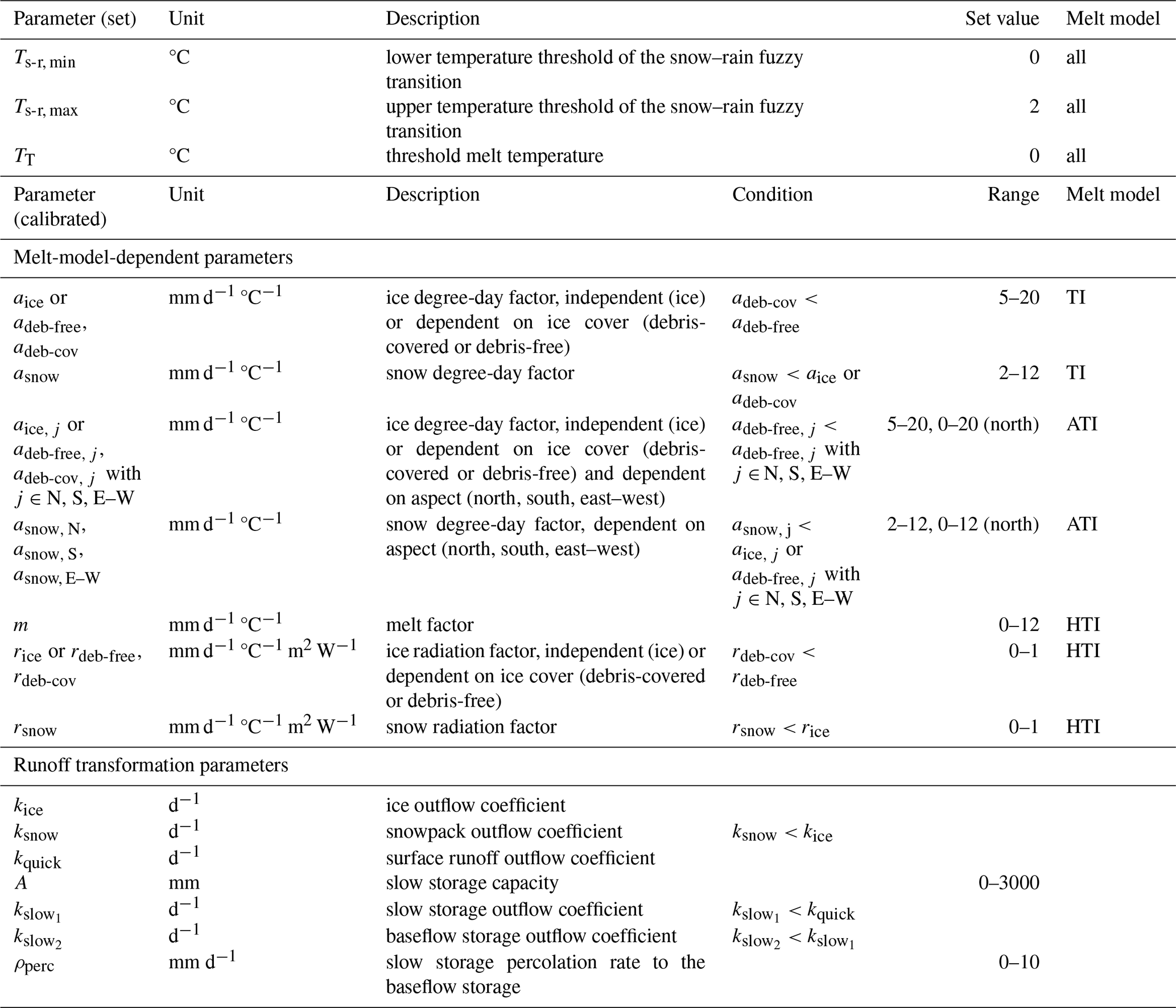
Table 3 Data used in the simulations, with corresponding source.

4 Results

4.1 Calibration runs

For the calibration runs without accounting for debris cover, the NSE and KGE values are better than the benchmark values for all catchments (Fig. 3; Sect. 3.4), implying a consistent enhancement in streamflow modeling with Hydrobricks compared to a simple temporal transfer of observed data. This improvement is more pronounced in smaller catchments, as the values of the benchmark metrics decrease with decreasing catchment area, while the Hydrobricks simulation scores remain consistently high. This suggests that in smaller catchments, discharge time series present more variable and marked yearly signals than in bigger catchments, which can be effectively replicated using Hydrobricks but not with resampling. Given that, in general, KGE values tend to be higher than NSE values (Knoben et al., 2019), this trend is particularly apparent with the benchmark NSE and slightly less with the benchmark KGE. Thus, even though the achieved NSE values are often lower than those of KGE, the improvement they represent compared to the benchmark metric values is much bigger.

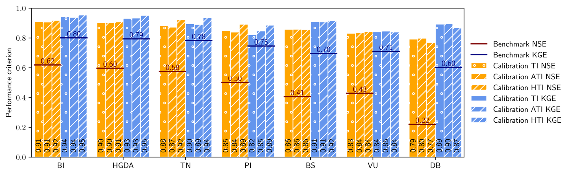
Figure 3 Comparison of the performance of the three melt models for the seven catchments for the period 2010–2014, quantified either by the Nash–Sutcliffe efficiency (NSE, orange bars) or the Kling–Gupta efficiency (KGE, blue bars). For comparison, the benchmark NSE and KGE are computed and plotted as red and dark blue thresholds. The model is calibrated by running 10 000 times over the years 2009–2014, where 2009 is discarded for model initialization. Catchments are ordered by area, from BI (largest) to DB (smallest). BI's nested catchments are underlined.

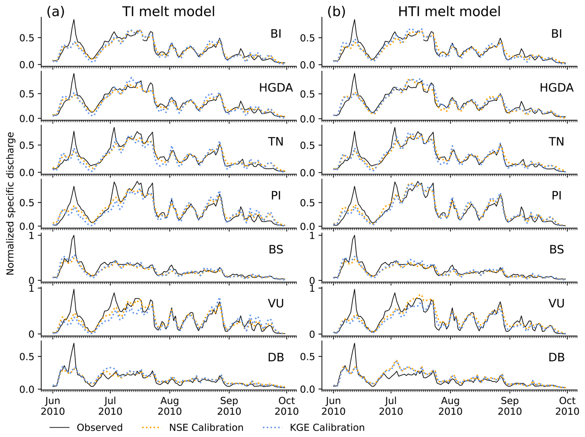
Figure 4 Observed and simulated hydrographs for all catchments for 2010 with the (a) TI and (b) HTI melt models. Observed discharge (solid black line) is compared to the calibration run using NSE (dotted orange) and KGE (dotted blue). Specific discharge (unit: mm) is normalized to the highest value.

To illustrate how well the calibrated discharge simulations fit the observed discharge, Fig. 4 shows the corresponding hydrographs. The calibration runs based on NSE and KGE (Fig. 4) result in globally similar hydrographs for the TI and HTI melt models, as well as for the ATI model (Supplement Fig. S4). While overall discharge dynamics are well simulated, some discharge peaks are smoothed and thus not adequately reproduced. This is particularly evident in the case of the “spring event” occurring in early to mid-June. This first prominent peak during the melting season results from the melt of the supraglacial and hillslope snowpacks that occurred due to an unusually strong foehn on 9 and 10 June (Zbinden et al., 2010). This foehn event is only partially captured in the temperature records of the period, and none of the melt models account for wind, which is why this peak could not be reproduced entirely.

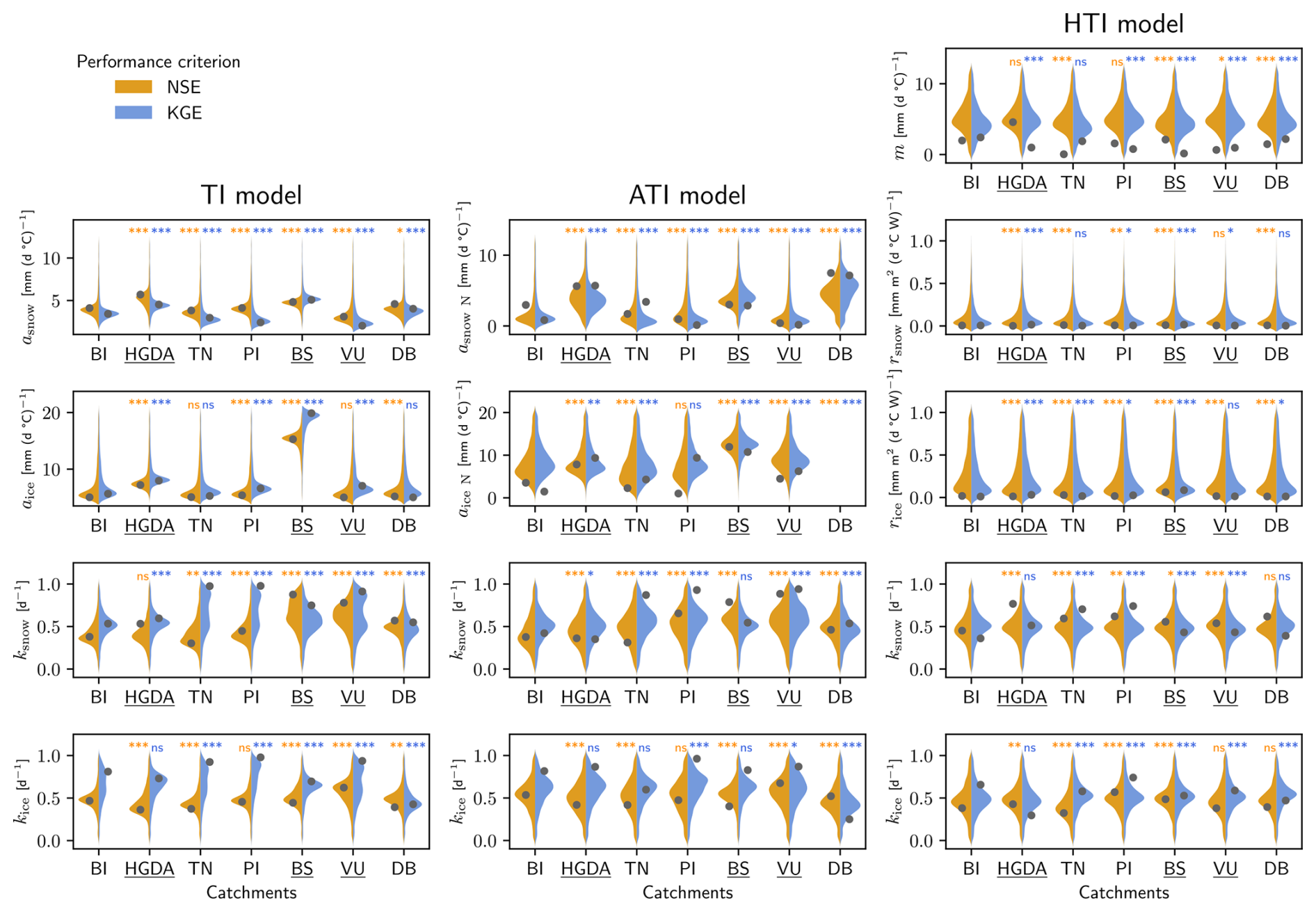
Figure 5 Calibrated ice melt and snowmelt parameters for all simulated NSE and KGE runs for all catchments, with the three melt models and the two performance criteria. The parameter sets achieving the best NSE and KGE scores are plotted on top with a dot. Catchments are ordered by area, from BI (largest) to DB (smallest). The significance of the parameter distribution difference between BI and its neighboring and nested catchments is denoted as follows: ${}^{***}$ for p<0.001, ${}^{**}$ for p<0.01, ^* for p<0.05, and ns for nonsignificant (Kruskal–Wallis test). BI's nested catchments are underlined.

The variability of calibrated parameters between performance criteria and between catchments depends on the melt model used (Kruskal–Wallis test; Fig. 5). Some models produce more pronounced variations, while others generate more limited variations. With the TI model, the calibrated parameter sets show very different values, depending on the catchment and the performance criterion used. With the ATI model, the degree-day factors and outflow coefficients obtained with KGE and NSE tend to converge to similar values, but these values still show a certain spread between the catchments. With the HTI model, all parameter values are more consistent between the two performance criteria and across the seven catchments. For example, the HGDA catchment shows high similarity with the BI catchment for both the snow radiation factor r_snow and the ice radiation factor r_ice in NSE calibration (non significant distribution change – ns; Fig. 5).

Thus, refining the representation of the melt process leads to increased spatial coherence of the melt parameters. The parameters showing no significant distribution changes between catchments could be assumed to be transferable between these catchments without calibration. The HTI model can thus be assumed to be suitable to model the melt processes occurring in neighboring or nested catchments.

4.2 Transfer runs in nested catchments: spatial parameter transferability

To assess the spatial parameter transferability to nested subcatchments, we apply, for all melt models, the calibrated parameter set obtained for the BI catchment to model the discharge of its nested subcatchments BS, HGDA, and VI. The results for the TI and HTI models are shown in Fig. 6, and those for the ATI model are shown in Supplement Fig. S5; the transfer runs closely match the observed discharge for the TI and HTI models. For both models, the simulated discharges of the HGDA and BS catchments show slightly underestimated low flow periods and peaks. While this can be observed for HGDA throughout the summer, it is especially true for BS in the late summer. VU, on the contrary, shows slightly overestimated discharge in the low flows and the peaks, starting in July, and overall, its discharge is best reproduced by the TI model. Close inspection reveals some differences between the transfer runs based on NSE versus KGE calibration but no systematic differences.

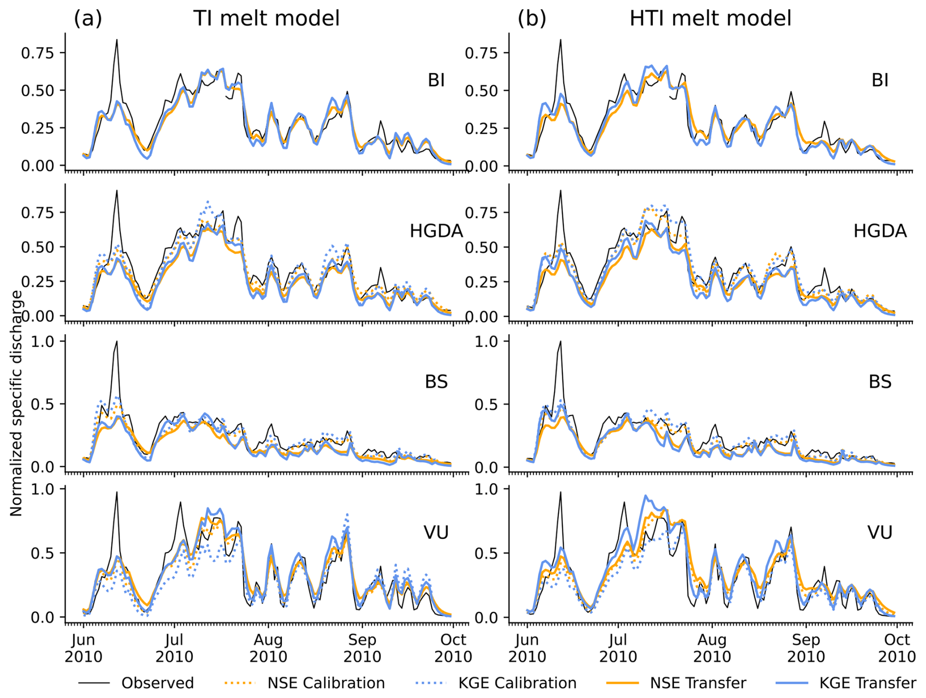
Figure 6 Observed and simulated hydrographs of the BI catchment and its nested subcatchments for 2010 with (a) TI and (b) HTI melt models. Observed discharge (solid black line) is compared to the calibration runs and to the transfer runs with the calibrated parameters of BI: shown are the results for NSE (orange) and KGE (blue); dotted lines show the calibration runs, and solid lines show the transfer runs. For BI, the calibration and transfer runs are identical. Specific discharge (unit: mm) is normalized to the highest value.

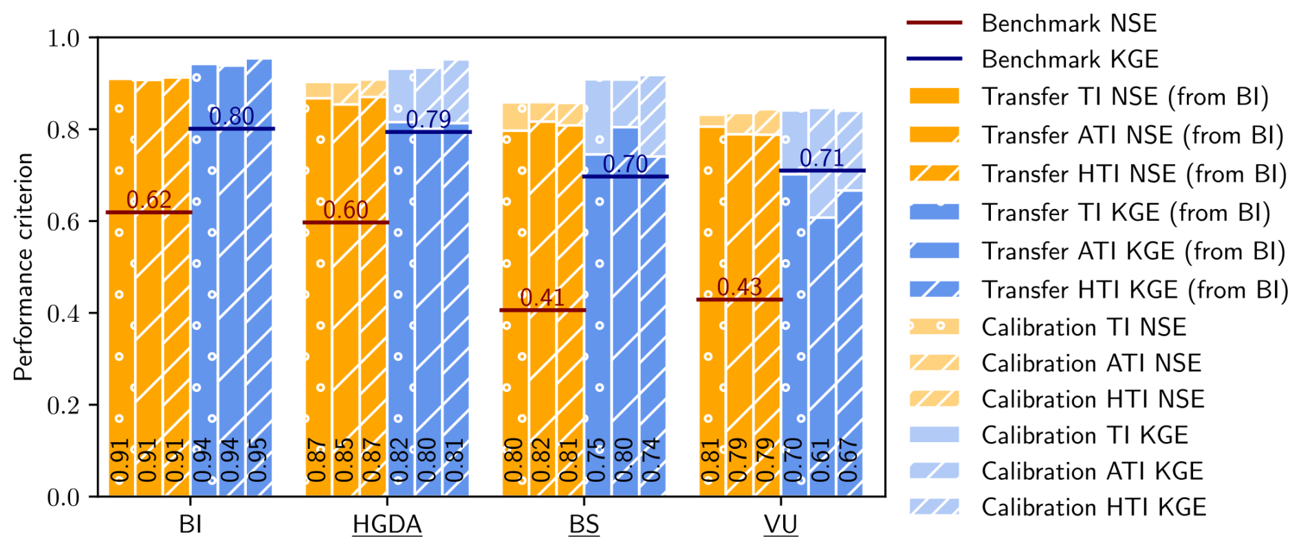
Figure 7 As Fig. 3 but comparing calibration and transfer runs for the subcatchments of BI for the period 2010–2014. Shown are NSE values (orange) and KGE values (blue), along with the benchmark NSE value (red line) and KGE value (dark blue line) values. The performance values for the corresponding calibration run are shown in more transparent color. BI's nested catchments are underlined.

As expected, the transfer runs reproduce the observed discharge less closely than the calibration runs for each of the catchments. The performance metric values of the transfer runs (Fig. 7) are, nevertheless, high compared to the benchmark values. Globally, the performance drop is larger for KGE than for NSE, but given the different sensitivities of the two metrics, they cannot be directly compared (see Sect. 4.1). Although all subcatchments and models experience a drop in KGE values, VU is the only catchment whose results drop just below the KGE benchmark value with all models. With the exception of the BS catchment, the best results are obtained with the TI and HTI models.

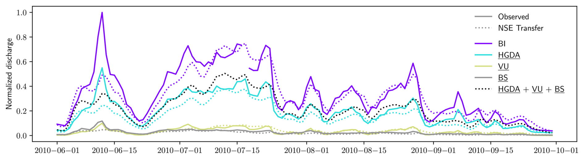
Figure 8 Observed and simulated hydrographs with the HTI model for the Bertol Inférieur (BI) and its subcatchments (VU, HGDA, and BS) for the summer of 2010. For the subcatchments, the simulations (dotted lines) are the NSE transfer runs. For the main catchment, BI, the dotted line corresponds to the calibration run. The solid lines are the observed hydrographs. The dotted black line shows the sum of the transfer runs of the three subcatchments. Discharge (unit: m³ s⁻¹) is normalized to the highest value. BI's nested catchments are underlined.

We tested the consistency of the model across scales by checking whether the simulated discharges of the subcatchments (VU, HGDA, and BS) were coherent across subcatchments and with the discharge of the main catchment (BI) (Fig. 8). This test is partial, as the discharge generated by the Mont Collon (MC) area is not monitored, and thus the added discharges of VU, HGDA, and BS do not account for all of BI's discharge. We thus expect the sum of the three subcatchments' discharges (dotted black line, Fig. 8) to always be lower than the discharge of the main catchment BI (dotted purple) and to have a consistent overestimation or underestimation of the flow across the different subcatchments. This is true for the high flow event triggered by the 9–10 June 2010 foehn event (Zbinden et al., 2010), which is consistently underestimated in all catchments. Similarly, we find that for the low flow periods at the end of June and early September, which are slightly overestimated in BI, the stacked discharges (dotted black) are consistent and stay below the BI discharge (dotted purple).

4.3 Transfer runs in neighboring catchments: spatial parameter transferability

The results of transferring the calibrated parameters of BI to neighboring catchments (Fig. 9, Supplement Fig. S6) demonstrate for 2010 high accuracy in discharge simulation with both the TI and HTI models, with minimal performance loss compared to calibration runs. The simulated discharge changes resulting from this forcing are more pronounced for the TI model than for the HTI model. Again, the discharge dynamics are relatively well reproduced but with a significant underestimation of the initial June discharge peak for all catchments and the July ones for the TN and PI catchments. Interestingly, the July peaks are absent in the observed discharge of the DB catchment (as they are absent in the observed discharge of the BS catchment; see Fig. 6). As seen in the nested forcing results (Fig. 6), the NSE calibration run fits the discharge peak sometimes better than the KGE calibration run, such as in catchment DB in early July with the TI model.

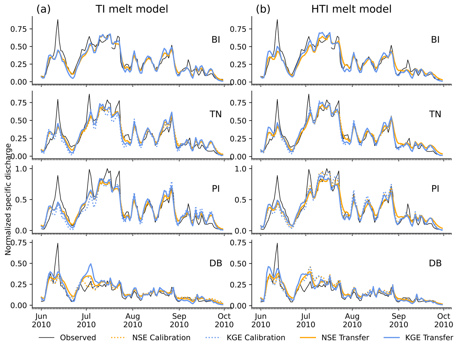
Figure 9 Observed and simulated hydrographs of the BI catchment and its neighboring catchments for 2010 with (a) TI and (b) HTI melt models. Observed discharge (solid black line) is compared to the calibration run and to the transfer runs with the calibrated parameters of BI: shown are the results for NSE (orange) and KGE (blue); dotted lines show the calibration runs, and solid lines show the transfer runs. For BI, the calibration and transfer runs are identical. Specific discharge (unit: mm) is normalized to the highest value.

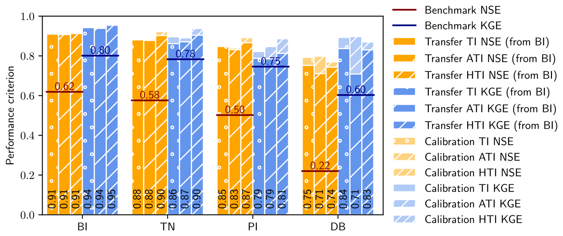
Figure 10 As Fig. 7 but comparing calibration and transfer runs for the neighboring catchments of BI for the period 2010–2014. Shown are NSE values (orange) and KGE values (blue), along with the benchmark NSE value (red line) and KGE value (dark blue line). The performance values for the corresponding calibration runs are shown in more transparent color.

We observe similar drops in NSE and KGE values when applying the BI parameters to the neighboring catchments similar as for the transfer runs in the BI subcatchments (compare Figs. 7 and 10). Nevertheless, with the exception of the DB catchment using the ATI melt model, the performance decreases are less pronounced compared to the nested catchments. In all neighboring catchments, the simulations exhibit NSE and KGE values that exceed those of the benchmark. Thus, the catchments whose discharges are the least well simulated with BI's calibrated parameters are the BI's nested subcatchments: VU, BS, and HGDA.

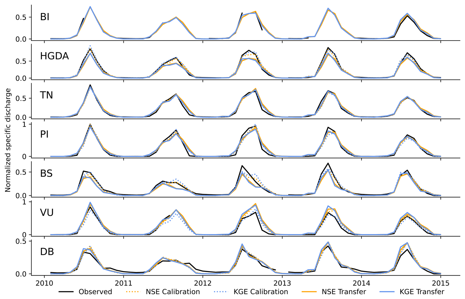
Figure 11 Observed and simulated monthly hydrographs for the HTI melt model for the seven catchments, calibrated or transferred with the calibrated parameter set of BI. Observed discharge (solid black line) is compared to the calibration run and to the transfer runs with the calibrated parameters of BI: shown are the results for NSE (orange) and KGE (blue); dotted lines show the calibration runs, and solid lines show the transfer runs. For BI, the calibration and transfer runs are identical. Observed monthly discharges with missing values are not shown. Specific discharge (unit: mm) is normalized to the highest value.

Analyzing monthly discharge hydrographs (Fig. 11) can yield additional insights into KGE performance, since this metric is by construction more sensitive to model biases than NSE, and such biases can become more apparent in monthly values compared to daily values. The monthly hydrographs (Fig. 11) clearly show the monthly discharge patterns that contribute to decreases in KGE, especially notable in 2012: in the VU catchment, discharge is overestimated, whereas in the HGDA and BS catchments, underestimations are observed.

4.4 Increased model complexity run: accounting for debris cover

In an attempt to investigate whether the melt model could be missing an important driving factor, we tried to attribute the performance decrease between calibration and transfer simulations to catchment characteristics. We chose to focus on the nested catchments, which show the largest drop in performance (Fig. 12). The catchment area and mean catchment elevation do not show any obvious relations to performance decreases. However, the percentage of glacier debris cover and the mean catchment and glacier slopes show more consistent relations. When the slope is steeper than in BI, discharge is underestimated, whereas when the slope is flatter, discharge is overestimated. In a similar way, when the debris coverage of the glacier is smaller than in BI, discharge is underestimated. Consequently, in the next step, we tested the transferability of model versions that differentiate between debris-covered and debris-free glacier areas.

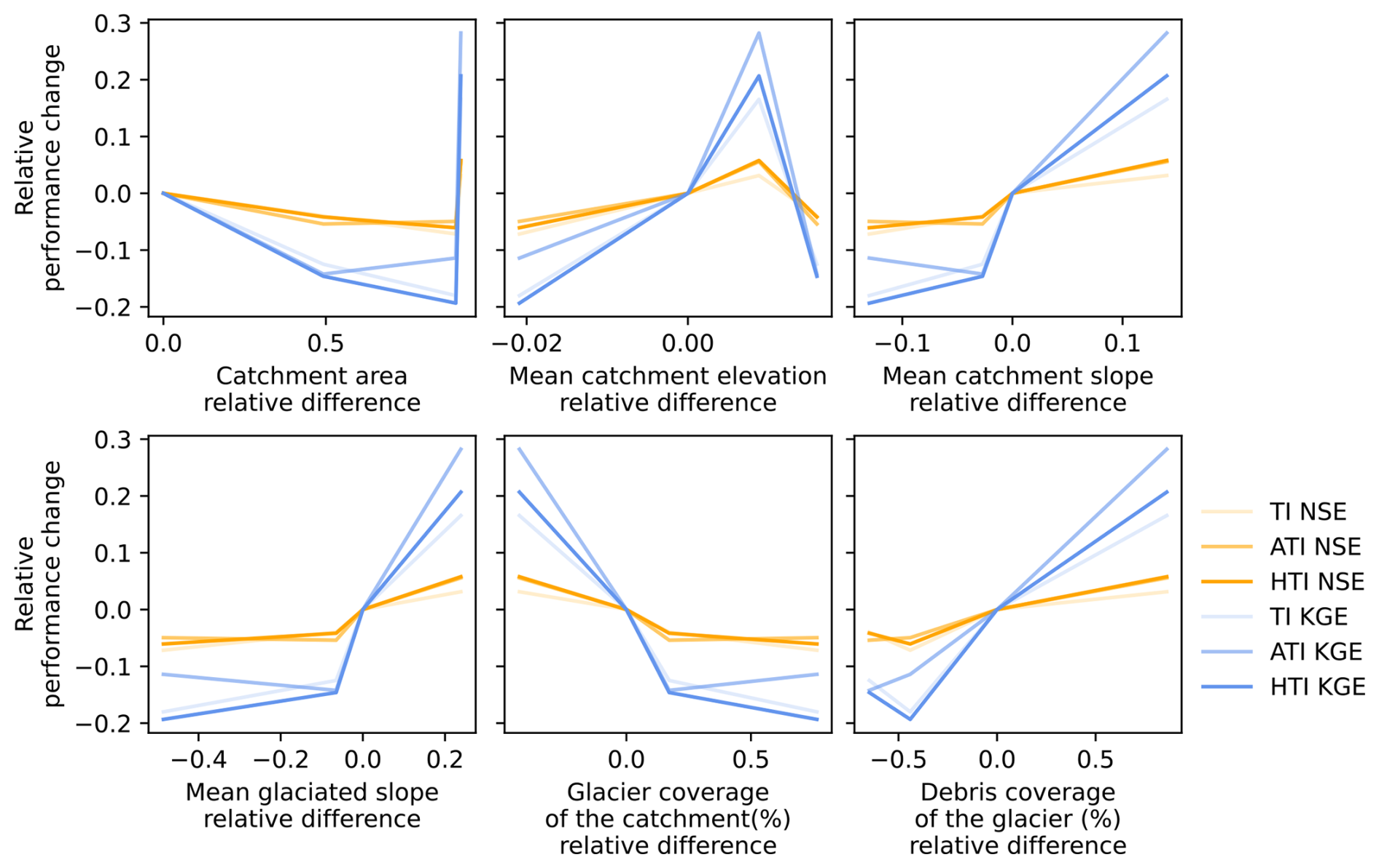
Figure 12 Comparison of selected physiographic characteristics of the nested catchments with the relative performance change between the calibration and transfer discharge simulations. The relative performance change is the relative drop in KGE and NSE performance criterion, calculated as follows: $(\text{calibration run}-\text{transfer run})/\text{calibration run}\times c$, with c a visually assessed coefficient reflecting the overestimation (1; VU) or the underestimation of simulated discharge (−1; HGDA and BS). The relative differences are calculated as follows, with the catchment area as an example: $(\text{BI catchment area}-\text{catchment area})/\text{BI catchment area}$. The point showing performance changes and relative differences of 0 is BI.

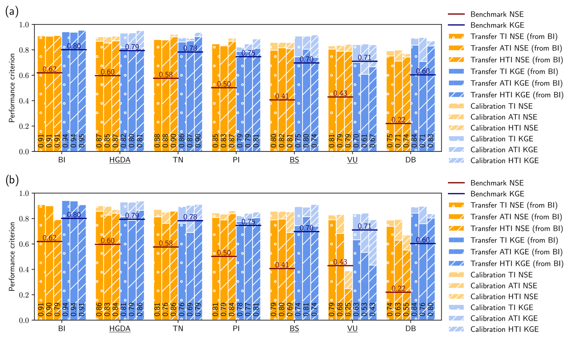
Figure 13 As Fig. 3 but comparing calibration and transfer runs for all seven catchments (a) without and (b) with debris cover separation for the period 2010–2014. Shown are NSE values (orange) and KGE values (blue), along with the benchmark NSE value (red line) and KGE value (dark blue line). The performance values for the corresponding calibration runs are shown in more transparent color. BI's nested catchments are underlined.

With model versions that apply different melt and radiation factors to simulate melt from debris-covered and debris-free glacier areas, we obtain better model performances in the calibration phase (see Fig. S8). However, for the transfer runs, the performances are lower than for model versions that do not account for debris cover (Fig. 13b); i.e., the transferability of the model parameters decreases. This is especially noticeable for the VU and TN catchments.

4.5 Regionalization of the melt model

We showed that with the TI and HTI models it is possible to simulate the discharge of nested and neighboring catchments with parameters calibrated at the main local outlet (BI), albeit with a small decrease in performance. The ensuing question is whether or not these parameters can be used to infer conclusions about the physical processes and dynamics occurring in the neighboring and subcatchments. In our simulations, the studied catchments have very similar meteorological drivers in terms of precipitation (Fig. 14a) and temperature (Fig. 14b). The meteorological data are interpolated based on ground-based observations from a few rather low-elevation measuring stations, with the only station in our study area being that of Arolla at 2005 m a.s.l. (Fig. 1a) and the highest station in the surrounding area being located 29 km SW at Col du Grand St-Bernard, at 2472 m a.s.l. Thus, the actual weather patterns may be more different between the studied subcatchments than is suggested by the interpolated weather data. Indeed, the studied catchments' discharge patterns show clear differences between DB and BS and the other catchments. DB and BS show for all years on record a single melt-induced discharge peak in early summer, followed by low discharge. All other catchments show the same discharge peak in June, followed by even higher discharges in the subsequent summer months (Fig. 14c).

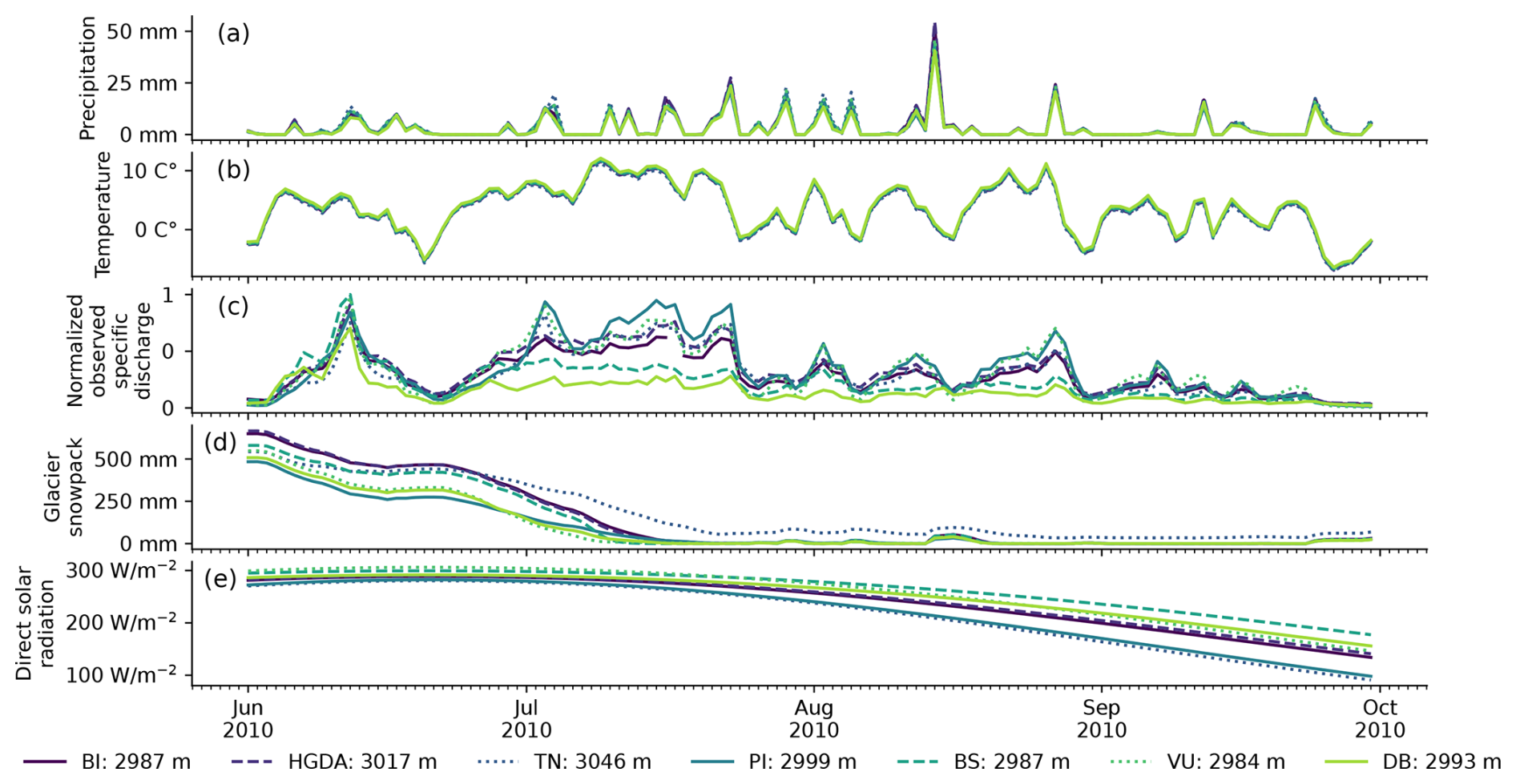
Figure 14 Patterns of (a) precipitation, (b) temperature, (c) observed discharges, (d) simulated glacier snowpack thickness, and (e) potential clear-sky direct solar radiation for the different catchments during the summer 2010. The values are mean values computed over the entire catchments from the RhiresD and TabsD MeteoSwiss datasets. The mean elevation of the catchment is indicated in the legend. Specific discharge (unit: mm) is normalized to the highest value.

To assess the quality and uncertainty of the precipitation inputs fed into the model, we compared the mean precipitation for each catchment with the measured precipitation from four weather stations: the Arolla station (2005 m a.s.l., since end of 2011 only), the Orzival (2640 m a.s.l.) and Tracuit (2590 m a.s.l.) stations from the Anniviers valley just to the east, and the Col du Grand St-Bernard station (2472 m a.s.l.) farther to the west. The precipitation inputs of our catchments globally fall within the same range as the measured precipitation of the Arolla station (Fig. S12c) in terms of annual precipitation amounts. The modeled interannual trend also matches the interannual trend observed in the neighboring Anniviers valley. At the daily scale, the peaks are globally well reproduced in terms of timing but are sometimes more uncertain in terms of amount (July 2012 peak; Fig. S12b). This discrepancy is explained by the high variability of precipitation in high alpine areas, which is well illustrated by the precipitation differences at large spatial scales between the Col du Grand St-Bernard and the Anniviers stations (Fig. S12a, c) and at smaller spatial scales between the two Anniviers stations (April 2012 peak; Fig. S12b). This small spatial-scale variability, however, has no impact on the global interannual trends (Fig. S12c). There is little variation in the amount of precipitation between our catchments (Fig. S12b), which leads us to believe that the spatial variability of our precipitation input is probably underestimated. This minimized variability of the input precipitation might explain the model's difficulty in reproducing specific discharge peaks and the distinctive hydrological regimes exhibited by DB and BS. Thus, some effects from rainfall variability that are not captured in the input data are possible.

Another reason may relate to the glacial coverage of the DB and BS catchments. Based on the simulated snow water content, we find that the lower discharges exhibited by BS and DB in July–August cannot be entirely explained by snow exhaustion, as BS and DB still show more than 10 cm of mean simulated snow depth at the beginning of July. However, they may be explained by the intra-annual pattern of snow and ice melt – when snowmelt slows due to depletion, glaciers become snow-free and ice melt begins. DB and BS show the lowest glacial coverage (<10.1 %; Table 1), so when the snow has disappeared, very little ice melt occurs. In other catchments, ice cover is much greater (>32.0 %), and in late July and early August, discharge is at its highest due to high rates of ice melt. We also note that TN is the only catchment for which the simulated snow cover did not melt completely during summer 2010 (Fig. 14d).

5 Discussion

5.1 An exhaustive block resampling benchmark

In this study, we have introduced a benchmark based on the bootstrapping method, where we exhaustively resample discharge data from the 5 years 2010–2014 in yearly blocks to simulate 3125 discharge time series, calculate the NSE and KGE objective functions for each of these time series, and average them. This resampling method was retained because it is an easy metric to compute and it gives a good idea of the model fit in comparison to a sample of discharge with the same hydrologic regime. Our catchments are all dominated by recurrent summer snowmelt and ice melt dynamics (Fig. S22), albeit with some temporal variability. To ensure that our benchmark is not affected by outlier years exhibiting significantly different dynamics, we computed a long-term benchmark over the whole available dataset (46 years; Table S4), which shows lower values of NSE and KGE than the 5-year benchmark, demonstrating the relative consistency of the dynamics in recent years.

5.2 Discharge predictability: catchment size matters

We first discuss the influence of catchment size on discharge predictability, notably on our benchmark metrics. The benchmark metrics show that the predictability of discharge from past discharge signals alone is lower for small catchments than for larger ones (Fig. 3). However, Hydrobricks shows similarly high model performances for small and larger catchments, highlighting the added value of a hydrological model in small catchments. This outcome can be directly explained by spatial relations. Large catchments exert a stronger averaging effect on spatiotemporal processes than small catchments. Indeed, the discharge in small catchments is driven by localized and likely uniform meteorological patterns, while larger catchments draw from multiple local meteorological patterns, leading to a certain averaging. This is well illustrated by the precipitation events in the Anniviers valley (Fig. S12b), which are not always recorded by both stations. This complexity obscures the correlation between meteorology and discharge in larger catchments, but not in smaller ones. Furthermore, the difference in catchment areas here is closely linked to differences in stream order, which results in a different balance between water travel times in unchanneled states (hillslopes, surface runoff) and in channeled states (in-stream) (Rinaldo et al., 2006; Michelon et al., 2021). Longer in-stream flow paths thereby lead to a stronger dampening effect of hillslope- and glacier-scale runoff variability. This geomorphological dispersion of the discharge waves traveling downstream (Rinaldo et al., 1991) can also be observed when comparing the discharge patterns recorded in the BI, VU, and HGDA intakes (Supplement Fig. S13): the smaller catchments (VU and HGDA) are relatively much more affected by the precipitation event than BI, even though they are hydrologically similar. Given the inherent year-to-year variability in meteorological patterns and the close link between meteorology and discharge, it follows that in small catchments, the discharge patterns from previous years are poor predictors of the current discharge. In contrast, even simple meteorology-based hydrological models such as Hydrobricks deliver much better results.

Additionally, we note that the NSE benchmark metric values tends to decrease much more strongly than the KGE benchmark metric values with decreasing catchment size (from 0.62 to 0.22 for NSE and from 0.80 to 0.60 for KGE; Fig. 3). This difference in decrease is explained by the resampling approach used to produce the discharge data. The NSE assesses the fit of one series to another solely based on the squared difference between the two time series. The KGE, on the other hand, uses a linear combination of correlation between the two series, variability error (ratio of the standard deviations), and bias error (ratio of the means). Given the definition of KGE and NSE, the correlation term is linearly related to NSE, whilst the variability term and the bias term have a quadratic relation to NSE (Clark et al., 2021). As a result, the NSE is much more sensitive to changes in variability or shifted yearly patterns than the KGE (see Sect. S9.1; Knoben et al., 2019). Furthermore, since the KGE evaluates bias, variability, and correlation independently, two good components (e.g., bias and variability) can offset a suboptimal third component (e.g., correlation). This is not the case in the NSE. Thus, the benchmark KGE values past discharges much more highly than the NSE, which makes it a much harder criterion to meet for simulated discharges than the benchmark NSE. We thus expect the simulated hydrographs to outperform the benchmark NSE and match the benchmark KGE.

5.3 Satisfactory hydrograph predictions across nested and neighboring catchments

As discussed previously, we expect the simulated hydrographs to outperform the benchmark NSE and match the benchmark KGE. When transferring the parameters calibrated for the largest subcatchment (BI) to model the discharge in all other nested (Fig. 7) and neighboring catchments (Fig. 10), we observe that despite exhibiting slightly inferior performance compared to the direct calibration, most catchments still show satisfactory results, even for the smallest ones. For all catchments, the transfer simulations with transferred parameters match both the benchmark KGE and NSE, with the exception of VU. The decreases in KGE for the HGDA, BS, and VU observed in all melt models is not accompanied by a similar NSE decrease, which hints toward an amplitude change in the discharge signal (Supplement Sect. S9.1). This amplitude change is produced by the underestimation (HGDA, BS) and overestimation (VU) of discharges that we observe in Fig. 6.

The lowest NSE score obtained through a HTI transfer run is 0.76, and the biggest decrease with respect to the calibration run reaches 0.05. As a comparison, the best fits achieved by Parajka et al. (2005) for regionalization over Austrian catchments yielded an NSE decrease from 0.72 to 0.67, and globally, the mean and maximum NSE in European catchments reach 0.72 and 0.91, respectively (Guo et al., 2021). Furthermore, the discharges in nested catchments are consistent with each other (Fig. 8), as the sum of the nested discharges does not exceed the main catchment's discharge.

The performance decrease between calibration and transfer simulations in nested catchments could be attributed to the slope of the terrain and the debris coverage of the glacier (Fig. 12). When the catchment and glaciated slopes are steeper, the models tend to underestimate discharge, maybe because steeper slopes lead to faster runoff and higher discharge rates that are not fully captured by the model. Conversely, for flatter slopes, the models overestimate discharge, possibly due to slower runoff and more significant water retention. Additionally, lower debris coverage on glaciers leads to underestimated discharge, potentially because debris cover, in our case, increases rather than decreases melt rates. By taking into account these relations between discharge and physiography explicitly in the model, we could potentially improve its transferability.

5.4 Possible explanations for slightly over- and underestimated discharges

Several factors could contribute to the overestimation of the VU discharge and to the underestimation of the HGDA and BS discharges observed in the monthly hydrographs (Fig. 11). Firstly, the meteorological forcing could be incorrect, as it is highly variable in such alpine environments, difficult to observe, and available at a coarse resolution (1 km). Calibrated parameters are known to compensate for such input error effects (Bárdossy and Das, 2008) and transferred parameters might thus induce biases. Secondly, the delineation of some of the catchments is uncertain, considering the uncertainty of water flow paths beneath glaciers. This might in particular be the case for VU, where Bezinge et al. (1989) suggest a potentially smaller catchment area to the north. Thirdly, the melt model could be missing an important driving factor. Temperature-index-based methods are known to yield good results in environments where melt is mainly driven by incoming longwave radiation and sensible heat flux (Ohmura, 2001), which is typically the case in alpine catchments (Thibert et al., 2018).

We also observe a worsened result when accounting for debris cover on glaciers. The following reasons might explain this result: (i) an overfitting of local specificities of the model, (ii) a spatially inconsistent effect of debris cover on ice melt, or (iii) difficulties making the high number of parameters converge given the amount of reference information contained in observed discharge (which does not provide enough constraints on the parameters). These reasons are linked. The inconsistent effect of debris (ii) when the “local specificity” is, for example, a strong melting or protective effect of the debris cover, which is not shared by other catchments, is a specific example of model overfitting. (i) Convergence difficulties (iii) lead to the difficulty of finding a single set of parameters to explain the results, which in turn can lead to an overfitting of local specificities if a solution is slightly better (i). All these reasons fall under the overparameterization problem.

We observe that in the cases of the ATI and the debris cover in TI and HTI, we introduce differential melt rates that cannot be independently calibrated as we only use the discharge to calibrate against. Compared to the simple TI model (without accounting for debris), the introduction of debris cover within the TI model results in a greater drop in goodness of fit than using the simple ATI model. Thus, we can conclude that this decrease in goodness of fit is probably due to the differential behavior of debris cover.

5.5 Enhanced parameter transferability through improved melt model accounting for potential solar radiation

Melt rates per positive degree day are sensitive to a number of characteristics that influence the surface energy balance and which include elevation, direct solar radiation input, albedo, wind speed, and seasonality (Hock, 2003; Ismail et al., 2023). These imply that for a given glacier, the degree-day factors of ice and snow are different, with ice, being less reflective than snow, melting more per positive degree day. This variability of the link between positive air temperature and melt can also be found at a local scale, within snow and ice patches (Gabbud et al., 2015). This sensitivity of melt rates tends to limit the transferability of melt parameters from one catchment to a neighboring or nested catchment for the basic TI model and motivated the computation of spatially variable degree-day factors from snow data in previous work (He et al., 2014; Hingray et al., 2010). Here, we tested the influence of aspect and radiation on melt model parameter transferability by discretizing the study catchment according to aspect and solar radiation and implementing the ATI and HTI models. According to the work of Comola et al. (2015), local-scale degree-day factors become stable (and therefore transferable) at scales at which the variability of local hillslopes' orientation does not further increase (less than 7 km² in their study). In this case study, we have five catchments that are small enough to be affected by their dominant aspect, but only two of them also show low aspect variance on their glaciated surfaces (DB and BS; Fig. 1c). However, all TI and ATI calibrated melt and radiation factors are highly inconsistent across catchments, whereas we find strong parameter overlaps between catchments for the HTI model (Fig. 5). Similar to the work of Comola et al. (2015), we find that taking into account solar radiation patterns using the HTI model does not fully explain the hydrological response variability at smaller catchment scales. Indeed, BS and HGDA tend to have higher melt parameters when calibrated alone (Fig. 5) and produce slightly underestimated discharge when transferred with BI's parameters (Fig. 6), responsible for their lower KGE values (Fig. 7a). The transfer results obtained from the HTI model do not demonstrate improvements in terms of simulated hydrographs compared to the TI model (Figs. 6 and 9), suggesting that the radiation as computed by Hock (1999) may not be enough to explain the KGE differences. However, both the TI and HTI models show good transferability in terms of metrics to even the smaller catchments (Figs. 7 and 10). Although Comola et al. (2015) showed that aspect significantly influences the calibration of degree-day factors for small catchments (<7 km²) with the TI model, we elaborate to conclude that the hydrographs obtained through regionalization are still very good fits for smaller, nested catchments. We find that parameter transferability to catchments below 7 km² in the TI and HTI model is a reasonable approximation but that the HTI model should be preferred due to the more consistent parameter calibration.

These differences could also be due to variations in ice albedo. Indeed, the glaciers in the studied catchments are not identical in terms of debris cover (Fig. 1). We thus tried to take the debris into account but failed to obtain better results in transfer runs (Fig. 13b), which hints towards a non-consistent behavior of the debris cover. This is very possible, as debris cover is known to either shield or amplify melting (Gabbud et al., 2015). We do not have information about the debris thicknesses in our study area, and the contribution of two processes as close as debris-free ice melt and debris-covered ice melt would be hard to constrain from discharge data only (Pokhrel et al., 2008). Thus, debris-cover-related parameters are less transferable than the global ice parameters.

5.6 Implications

Our analysis underlines the value of including potential radiation in the temperature-index model for spatial transferability of melt model parameters, a topic that has been neglected in previous studies and is worth being pursued further. It remains to be shown whether similar transferability of the HTI melt model can be expected in larger catchments (i.e., >500 km²; e.g., Hingray et al., 2010; Fatichi et al., 2015), although we expect this to be true for all catchments whose hydrological regimes are strongly influenced by snow and glaciers, provided, of course, that other geomorphological characteristics are relatively constant. Most likely, the added value of potential radiation decreases for increasing catchment sizes since the variability of aspects with increasing scale tends to a limit value that averages out the effect on melt (Comola et al., 2015). In addition, future work could focus on the benefit of including snow data to jointly calibrate the melt model parameters and other hydrological process parameters. This multi-signal calibration, on both flow and snow data, could reduce parameter equifinality (though not eliminate it Finger et al., 2011) and reduce parameter interdependency, as shown in the work by Ruelland (2024). This could further enhance the transferability of glaciohydrological models (Carenzo et al., 2009). This only holds if the melt model gives an adequate representation of the melt processes for a streamflow simulation model: a large body of literature on temperature-index modeling focuses on how to further improve such models, e.g., by analyzing how degree-day factors or melt factors vary along the melt season (Ismail et al., 2023, and references therein), by improving the parameterization of subdaily melt dynamics (Tobin et al., 2013), or by linking melt to other variables rather than the average daily air temperature (Follum et al., 2019; Nasab and Chu, 2021). For all these interesting developments, the question of how melt model improvements increase (or decrease!) the spatial transferability of the model should receive much more attention than in the past.

6 Conclusions

In this study, we tested the spatial transferability of melt models incorporating progressively more spatial information: a classical temperature-index melt model (TI), a temperature-index melt model based on aspect (ATI), and the temperature-index melt model of Hock (HTI). To do so, we calibrated each melt model over seven different catchments, then transferred the calibrated parameters of the main catchment to the three nested catchments and the three neighboring catchments.

The results show that for high alpine catchments, it is possible to spatially transfer relatively simple semi-lumped glaciohydrological models. We have demonstrated that our semi-lumped model (Hydrobricks) can successfully simulate discharge at several upstream points of the catchment after calibration to a single downstream observed discharge time series. This makes multi-point discharge simulation possible.

Although the best results in terms of transferability are achieved with the TI and HTI models, the highest consistency between parameters is achieved with the HTI model. This better convergence of parameters is witnessed both between the two performance metrics, as is also the case for the ATI model, and among the seven catchments. The inclusion of debris cover on glaciers does not produce better results and leads to model overparameterization. The NSE metric gives better calibration results than KGE when trying to fit the discharge peaks, but the benchmark KGE proves to be a harder, and thus more significant, criterion to meet and better reproduces the observed peaks. Thus, we find that the best framework to transfer parameters calibrated in the biggest local catchment to subcatchments and neighboring ones is by using the HTI model without debris cover.

Our simulations highlighted the possible influence of catchment and glaciated slopes, as well as debris cover percentage, on the overestimation and underestimation of discharge in transfer runs. Since the inclusion of debris cover led to overparameterization, future research should focus on the integration of these characteristics in more spatially informed ways.