Catchments do not strictly follow Budyko curves over multiple decades, but deviations are minor and predictable

Quantification of precipitation partitioning into evaporation and runoff is crucial for predicting future water availability. Within the widely used Budyko framework, which relates the long-term aridity index to the long-term evaporative index, curvilinear relationships between these indices (i.e. parametric Budyko curves) allow for the quantification of precipitation partitioning under prevailing climatic conditions. A common assumption is that movement along a specific Budyko curve with changes in the aridity index over time can be used as a predictor for catchment responses to changing climatic conditions. However, various studies have reported deviations around these curves, which raises questions about the usefulness of the method for future predictions. To investigate whether parametric Budyko curves still have predictive power, we quantified the global, regional, and local evolution of deviations of catchments from their parametric Budyko curves over multiple subsequent 20-year periods throughout the last century based on historical long-term water balance data from over 2000 river catchments worldwide. This process resulted in up to four 20-year distributions of annual deviations from the long-term mean parametric curve for each catchment. To use these distributions of deviations to predict future deviations, the temporal stability of these four distributions of deviations was evaluated between subsequent periods of time. On average, it was found that the majority (62 %) of study catchments did not significantly deviate from their expected parametric Budyko curves. Out of the remaining 38 % of catchments that deviated from their expected curves, the long-term magnitude of median deviations remains minor, with 70 % of catchments falling within the range of ±0.025 of the expected evaporative index. When these median deviations were expressed as relative changes in discharge, catchments in arid regions showed higher susceptibility to larger discharge shifts compared to those in humid regions. Furthermore, a significant majority of catchments, constituting around the same percentage, was found to have stable distributions of deviations across multiple time periods, making them well suited to statistically predict future deviations with high predictive power. These findings suggest that while trajectories of change in catchments do not strictly follow the expected long-term mean parametric Budyko curves, the deviations are minor and quantifiable. Consequently, taking into account these deviations, the parametric formulations of the Budyko framework remain a valuable tool for predicting future evaporation and runoff under changing climatic conditions within quantifiable margins of error.

1 Introduction

Climate change is likely to have a profound impact on future global water resources (Jaramillo et al., 2018; Xing et al., 2018) by causing major shifts in the water balance of river basins worldwide (Serpa et al., 2015; Hattermann et al., 2017). Robust quantitative estimates of future water resources are therefore required to develop policies and to design engineering interventions that will allow the mitigation of the potentially adverse effects of these shifts on the water supply (Destouni et al., 2013).

From the early 20th century onwards, multiple authors have suggested analytical, functionally similar non-parametric, curvilinear relationships that describe the long-term average partitioning of precipitation into runoff and evaporative fluxes in terrestrial hydrological systems (Schreiber, 1904; Oldekop, 1911; Budyko, 1948). In spite of differences in their detailed mathematical formulation (Arora, 2002; Andréassian et al., 2016), all these relationships allow for mapping the long-term mean fraction of precipitation P that is evaporated, i.e. the evaporative index $I_{\mathrm{E}}=E_{\mathrm{A}}/P$, onto the long-term mean ratio of energy input, expressed as potential evaporation E_P, over precipitation, referred to as the aridity index $I_{\mathrm{A}}=E_{\mathrm{P}}/P$. Many studies have demonstrated that the empirical evaporative index I_E of river catchments worldwide indeed scatters rather narrowly around these non-parametric Budyko curves (Turc, 1954; Budyko, 1961; Choudhury, 1999; Zhang et al., 2001; Donohue et al., 2007; Berghuijs et al., 2014; van der Velde et al., 2014; Andréassian et al., 2016; Jaramillo et al., 2018; Reaver et al., 2022). To better account for the scatter, several parametric reformulations of the non-parametric Budyko curves have been proposed (Turc, 1954; Mezentsev, 1955; Tixeront, 1964; Fu, 1981). These one-parameter formulations were shown to be functionally almost equivalent to each other (Yang et al., 2008). Their parameter, hereafter referred to as ω, defines catchment-specific parametric Budyko curves that locate each catchment on a uniquely defined position in the space spanned by I_A and I_E, i.e. the Budyko framework. The ω parameter is widely interpreted to encapsulate all combined properties of a catchment that may influence the storage, and release of water other than I_A (Milly, 1994; Donohue et al., 2012; Shao et al., 2012).

The fact that the long-term water balance exhibits such a relatively consistent behaviour across a wide spectrum of hydroclimatically and physiographically distinct environments has led to the hypothesis that the general shape of Budyko curves emerges for natural systems in a co-evolution of climate, soil water storage and vegetation properties (Milly, 1994; Porporato et al., 2004; Donohue et al., 2012; Gentine et al., 2012; Troch et al., 2013). Consequently, it may plausibly be assumed that once equilibrium is reached after a change in I_A, the water partitioning in a catchment converges towards a new but predictable stable state (here I_E) by following its catchment-specific parametric Budyko curve defined by ω. By extension, such a space–time symmetry under a changing climate may then allow for estimates of future I_E and thus of E_A and Q based on changes in I_A, which are inferred from future projections of P and E_P (Roderick and Farquhar, 2011; Wang et al., 2016; Liu et al., 2020; Bouaziz et al., 2022).

However, parametric Budyko curves and their ω parameters were originally not developed from physical reasoning but rather from a largely process-agnostic, mathematical perspective with the aim to statistically describe observed data. They, therefore, do not have a clearly defined physical meaning, and the interaction of actual processes that control ω in specific environments is poorly understood. Consequently, mechanistic evidence that supports the space–time symmetry hypothesis remains erratic. This poses a serious obstacle for the formulation of a general mechanistic description to quantitatively and mechanistically link ω of parametric Budyko curves (and thus I_E) to catchment properties other than I_A (Xu et al., 2013; Padrón et al., 2017). This further entails that estimates of ω and the associated I_E for ungauged catchments or future climate conditions may be subject to major uncertainties and should therefore be interpreted from a probabilistic perspective (Greve et al., 2015).

Recently, it was also argued that catchments should not be necessarily expected to follow their long-term average, catchment-specific parametric Budyko curves, when subject to climatic perturbations expressed as changes in I_A (Berghuijs and Woods, 2016; Jaramillo et al., 2018, 2022; Reaver et al., 2022). Such deviations (ε_IEω) from the expected parametric Budyko curve are here defined as the dimensionless absolute difference between the observed evaporative index (I_E,o) and the predicted evaporative index (I_E) derived from the expected parametric Budyko curve. They were previously referred to as residual or landscape-driven, indicating that many factors other than I_A, such as human-induced changes in water and land use (e.g. afforestation, deforestation, irrigation, reservoir construction) also play a role (Donohue et al., 2007; Wang and Hejazi, 2011; Sterling et al., 2012; Destouni et al., 2013; van der Velde et al., 2014; Jaramillo and Destouni, 2015; Levi et al., 2015; Nijzink et al., 2016; Daly et al., 2019; Gan et al., 2021; Hrachowitz et al., 2021). As a consequence, Reaver et al. (2022) have warned that parametric Budyko curves may have no predictive power at all. This may be too pessimistic of a perspective. First, the average magnitudes of ε_IEω so far reported in studies remain rather low (e.g. Tempel et al., 2024; Wang et al., 2024). Second, there is increasing evidence that estimates in water yield are much less sensitive to fluctuations in ω (and thus ε_IEω) than to changes in precipitation, in particular for humid environments (Roderick and Farquhar, 2011; Berghuijs et al., 2017). Yet, as the assumption of steady conditions might not be applicable (Mianabadi et al., 2020), the presence of uncertainties in the modelling process is inevitable (Westerberg et al., 2011; Nearing et al., 2016). In other words, some level of deviation from the parametric Budyko curves is to be expected as different time periods will never be characterized by exactly the same environmental conditions. However, the mechanistic processes that control these deviations, and thus ω, are not well understood.

Although part of several previous analyses (Destouni et al., 2013; van der Velde et al., 2014; Berghuijs and Woods, 2016; Jaramillo et al., 2022; Reaver et al., 2022), to our knowledge, there has been no systematic, in-depth analysis of the distributions of ε_IEω or its evolution over multiple time periods at global, regional, and local scales explicitly reported in the literature. Jaramillo and Destouni (2014), Jaramillo et al. (2018) and Tempel et al. (2024) provided estimates of average ε_IEω for several regions but limited their analyses to two independent time periods, while Wang et al. (2024) analysed distributions of ε_IEω over multiple decades in one single river basin. In contrast, Reaver et al. (2022) quantified ε_IEω over multiple time periods but explicitly reported only estimates of ε_IEω maxima for individual catchments, thus describing merely the most extreme situations.

Our research question is whether the distributions and average magnitudes of ε_IEω remain stable and thus probabilistically predictable over time under changing environmental conditions in space and time. A positive answer to this question would imply that parametric Budyko curves can indeed be, at least over timescales of several decades, considered useful for predicting future I_E under changing conditions within quantifiable margins of error. Based on historical long-term water balance data from >2000 river catchments worldwide, we here quantify the distributions of deviations of catchments from parametric Budyko curves, i.e. ε_IEω, at global, regional, and local scales between multiple 20-year periods throughout the 20th century. Specifically, we test the hypothesis that the distributions of ε_IEω are too wide and temporally too unstable, so I_E from parametric Budyko curves needs to be considered practically unpredictable with the available data.

2 Datasets and methods

2.1 Meteorological and hydrological data

Daily precipitation P [mm d⁻¹] as well as maximum and minimum temperature T [°C] data at a spatial resolution of 0.5°×0.5° were obtained from the Global Soil Wetness Project Phase 3 (GSWP-3); (Dirmeyer et al., 2006) and spatially averaged for each study catchment over the time period of 1901–2015.

Potential evaporation, E_P [mm d⁻¹], was estimated based on the method proposed by Hargreaves and Samani (1982):

$$\begin{array}{}\text{(1)}& E_{\mathrm{P}}=\mathit{\alpha }{R}_{\mathrm{a}}(T_{\mathrm{a}}+\mathrm{17.8})\sqrt{(T_{\text{max}}-T_{\text{min}})},\end{array}$$

where α∼0.0023 is a constant used to convert $\mathrm{MJ}{\mathrm{m}}^{-\mathrm{2}}{\mathrm{d}}^{-\mathrm{1}}$ to mm d⁻¹; R_a is the extraterrestrial radiation at the top of the atmosphere [$\mathrm{MJ}{\mathrm{m}}^{-\mathrm{2}}{\mathrm{d}}^{-\mathrm{1}}$]; and T_a, T_max, and T_min are the daily average, maximum and minimum temperatures [°C], respectively. R_a is estimated using the method proposed by Duffie and Beckman (1980).

In this study, we obtained annual river flow data from the Global Streamflow Indices and Metadata Archive (GSIM; Do et al., 2018a; Gudmundsson et al., 2018a), which consists of in situ streamflow observations data for over 30 000 gauging stations worldwide. We selected stations with runoff data spanning at least 50 years in the 1901–2015 period, excluding those with a data quality flag labelled Caution. After filtering, we retained 2387 river catchments with data series ranging from 50 to 100 years (with a median of 78 years). These catchments vary in size, from 4 to 3 475 000 km² (with a median of ∼1564 km²; Fig. 1a). The catchments represent diverse hydroclimatic conditions (Fig. 1b–f), as indicated by the long-term average aridity index (I_A) that ranges from 0.19 to 6.66 (with a median of 0.97; Fig. 1e) and evaporative index (I_E) that ranges from 0.06 to 0.99 (with a median of 0.65; Fig. 1f).

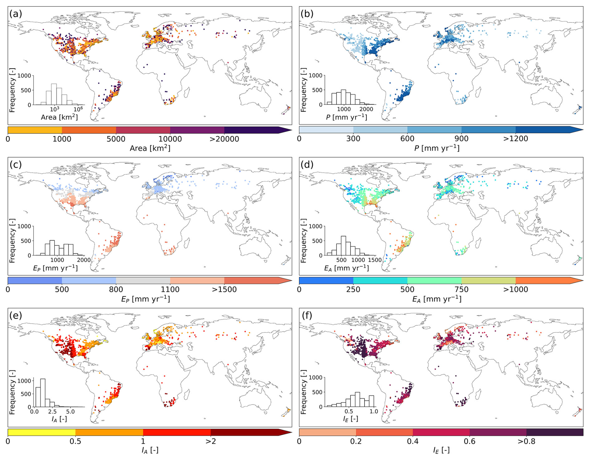
Figure 1 Spatial distribution of 2387 studied catchments along with topographic characteristics and long-term mean (1901–2015) climatic indices: (a) catchment area; (b) precipitation, P; (c) potential evaporation, E_P; (d) actual evaporation, $E_{\mathrm{A}}=P-Q$; (e) aridity index, I_A; and (f) evaporative index, I_E.

2.2 Methods

The subsequent experiment to estimate for each of the 2387 study catchments the deviation ε_IEω values from its expected evaporative index I_E over multiple subsequent time periods is based on the parametric Tixeront–Fu reformulation of the Budyko hypotheses (Tixeront, 1964; Fu, 1981), as illustrated in Fig. 2.

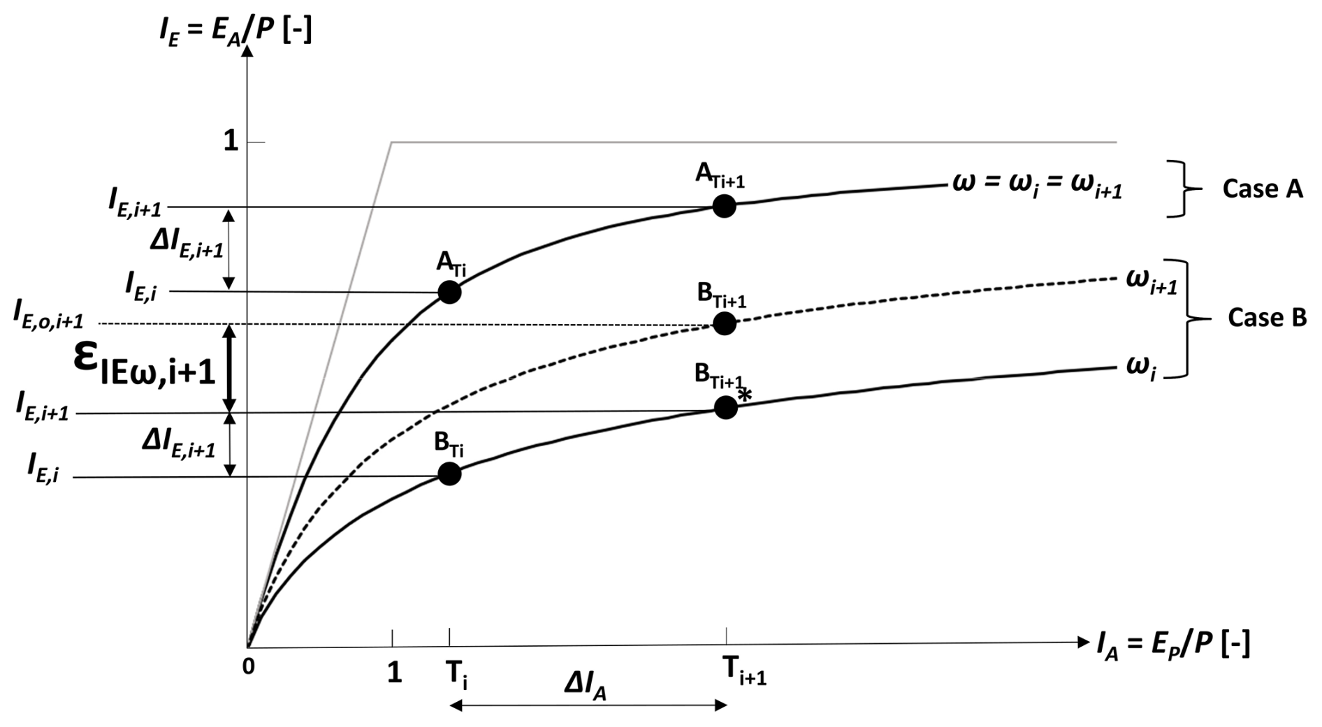
Figure 2 A schematic representation of a catchment movement in Budyko space between two long-term time periods, T_i and T_i+1. Case A: catchment A moves along the same Budyko curve from the first period T_i to the next period T_i+1 (i.e. ${\mathit{\omega }}_i={\mathit{\omega }}_{i+\mathrm{1}}$). Case B: catchment B has deviated from its expected parametric Budyko curve (i.e. ${\mathit{\omega }}_i\ne {\mathit{\omega }}_{i+\mathrm{1}}$), resulting in deviation ${\mathit{\epsilon }}_{\text{IE}\mathit{\omega },i+\mathrm{1}}$ (Eq. 4).

This movement in Budyko space is governed by the following equation:

$$\begin{array}{}\text{(2)}& I_{\mathrm{E}}={\displaystyle \frac{E_{\mathrm{A}}}{P}}=\mathrm{1}+{\displaystyle \frac{E_{\mathrm{P}}}{P}}-{\left[\mathrm{1}+{\left({\displaystyle \frac{E_{\mathrm{P}}}{P}}\right)}^{\mathit{\omega }}\right]}^{\frac{\mathrm{1}}{\mathit{\omega }}},\end{array}$$

where ω is a catchment-specific parameter estimated from long-term averages of observed P, E_P, and $E_{\mathrm{A}}=P-Q$, assuming negligible change in storage $\mathrm{d}S/\mathrm{d}t$.

Equation (2) suggests that with a given ω, hydroclimatic shifts between two periods, T_i and T_i+1, expressed as changes in aridity index $\mathrm{\Delta }{I}_{\mathrm{A}}=\mathrm{\Delta }(E_{\mathrm{P}}/P)$, will lead to predictable change $\mathrm{\Delta }{I}_{\mathrm{E},i+\mathrm{1}}$ (Case A). In other words, catchments will follow their specific curves in period T_i+1, defined by parameter $\mathit{\omega }={\mathit{\omega }}_i={\mathit{\omega }}_{i+\mathrm{1}}$, to an expected new $I_{\mathrm{E},i+\mathrm{1}}$, which is expressed as

$$\begin{array}{}\text{(3)}& I_{\mathrm{E},i+\mathrm{1}}=I_{\mathrm{E},i}+\mathrm{\Delta }{I}_{\mathrm{E},i+\mathrm{1}}\mathrm{\text{(Case A in Fig. 2)}}.\end{array}$$

However, in reality, as described above, ω is often not constant over time (Case B). Catchments therefore do not strictly follow their I_E,i curve defined by ω_i (from T_i) in a subsequent period T_i+1. For period T_i+1, this therefore leads to additional deviation ${\mathit{\epsilon }}_{\text{IE}\mathit{\omega },i+\mathrm{1}}$, which is described as

$$\begin{array}{}\text{(4)}& {\mathit{\epsilon }}_{\text{IE}\mathit{\omega },i+\mathrm{1}}=I_{\text{E,o,}i+\mathrm{1}}-I_{\mathrm{E},i+\mathrm{1}}\ne \mathrm{0},\end{array}$$

representing the difference between the actually observed I_E,o,i+1 from the expected $I_{\mathrm{E},i+\mathrm{1}}$. Thus, for period T_i+1, the observed I_E,o,i+1 depends on the combination of the predicted change and these deviations, i.e. the following applies:

$$\begin{array}{}\text{(5)}& I_{\text{E,o,}i+\mathrm{1}}=I_{\mathrm{E},i}+\mathrm{\Delta }{I}_{\mathrm{E},i+\mathrm{1}}+{\mathit{\epsilon }}_{\text{IE}\mathit{\omega },i+\mathrm{1}}\mathrm{\text{(Case B in Fig. 2)}}.\end{array}$$

Here, we have sub-divided the available data records of each catchment into up to five individual 20-year periods over the last century, denoted as T_i (Table 1), where T_i represents the ith 20-year period. This 20-year period was chosen deliberately to balance the need for a sufficiently long period to minimize the impact of storage changes while preserving the temporal sequence in the data that allowed us to place each catchment into a specific temporal stability category (as described in Step 4). We assume that 20-year periods are long enough to satisfy $\mathrm{d}S/\mathrm{d}t\approx \mathrm{0}$, which is supported by Han et al. (2020), who demonstrated that in more than 80 % of catchments worldwide, $\mathrm{d}S/\mathrm{d}t$ is less than 5 % over 20-year periods. Using longer periods, such as 30 years, as used in previous studies (e.g. Destouni et al., 2013), would have smoothed out potential shifts and limited the ability to detect systematic changes. In addition, 20-year periods align with planning horizons in many water resources management decisions.

Table 1 Symbols used in this study to present 20-year periods (T_i), changes between subsequent 20-year periods and distributions of deviations.

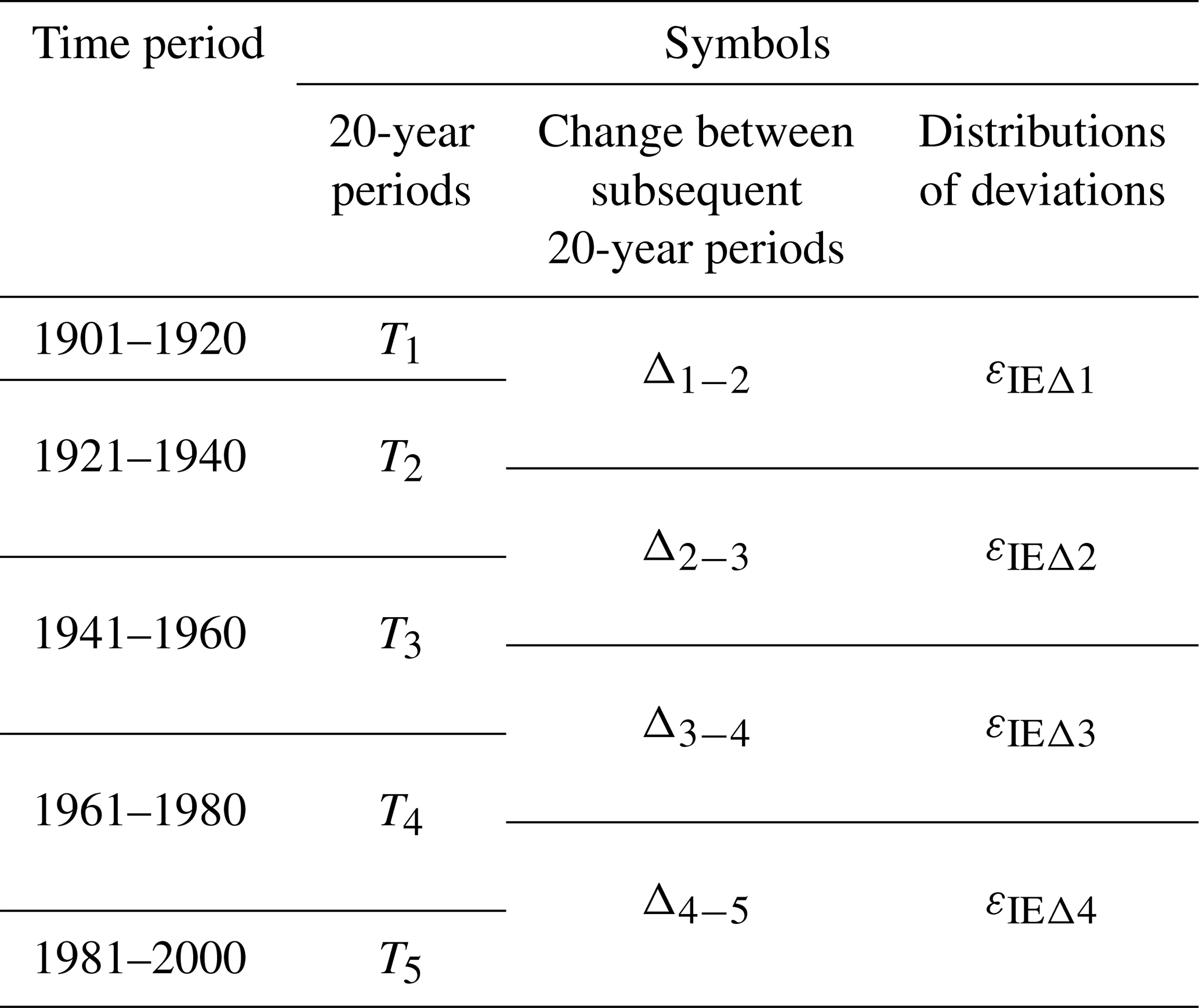
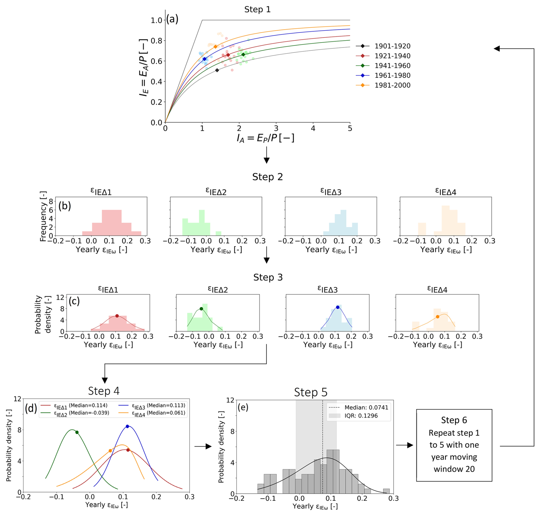
Figure 3 Flow chart of methodology. Step 1: estimation of catchment-specific I_E,i curves and the distribution of annual I_E,o around it for each period T_i. Step 2: distributions of annual deviations ε_IEΔj from expected $I_{\mathrm{E},i+\mathrm{1}}$ between subsequent time periods. Step 3: fitting parametric distributions to the empirical distributions of annual deviations ε_IEΔj. Step 4: evaluating temporal stability of the distributions ε_IEΔj in subsequent pairs of time periods. Step 5: aggregated long-term marginal distribution of annual deviation ε_IEω values from expected I_E for each catchment. Step 6: evaluation of the sensitivity of the marginal distributions of annual deviation ε_IEω values to the choice of 20-year averaging window. Note that the generated distributions of ε_IEω are illustrative examples that are not based on real data.

The experiment to estimate deviation ε_IEω values between the five individual periods T₁–T₅ for the study catchments was then carried out in a systematic sequence of five specific steps as illustrated in Fig. 3 and described in the following.

Step 1 – estimation of catchment-specific I_E,i curves and the distribution of annual I_E,o around it for each period T_i.

For each catchment and each individual 20-year time period T_i, the catchment-specific parametric Budyko curve I_E,i defined by parameter ω_i is obtained by fitting Eq. (2) to the set of 20 annual values of each catchment in the Budyko space as computed from the observed water balance data. The decision to obtain the ω_i for each 20-year period by fitting Eq. (2) to the set of n=20 corresponding observed annual I_E,o values instead of directly to their 20-year averages was a deliberate choice. The fluctuations in the n=20 annual I_E,o values explicitly represent annual storage changes ($\mathrm{d}S/\mathrm{d}t$) between individual years. This subsequently allowed us to treat the observed annual I_E,o probabilistically as distributions around their expected values for that period T_i as defined by I_E,i curve (Fig. 3a).

Step 2 – distributions of annual deviations ε_IEΔj from expected $I_{\mathrm{E},i+\mathrm{1}}$ between subsequent time periods.

For each catchment, we then used ω_i from each time period T_i to compute the expected $I_{\mathrm{E},i+\mathrm{1}}$ for the subsequent period T_i+1 (i.e. point B_Ti+1* in Fig. 2). This then allowed us to estimate the individual deviations of the 20 annual observed I_E,o values from the expected $I_{\mathrm{E},i+\mathrm{1}}$ curve. For each pair of time periods T_i–T_i+1 (i.e. T₁–T₂, T₂–T₃, etc., hereafter referred to as Δ₁₋₂, Δ₂₋₃, etc.), this resulted in an individual distribution of annual deviation ε_IEω values around a 20-year average in each catchment (Fig. 3b). This approach using a temporally changing (dynamic) baseline was chosen as it is more sensitive for capturing trends and shifts in hydrological behaviour of catchments over time than a fixed baseline. For completeness, we also performed the same analysis using a fixed baseline (i.e. using the earliest available period as a fixed baseline) and provide the results thereof in the Supplement.

Note that catchments with data for all five time periods T₁–T₅ have the maximum of j=4 distributions ε_IEΔj. In contrast, catchments with data for only two periods, e.g. T₂ and T₃, feature only j=1 distribution of between-period deviation ε_IEω values.

Non-parametric Wilcoxon signed rank tests were then used to test for each distribution ε_IEΔj the null hypothesis that the median deviation is not significantly different from zero. The lower the p value, the higher the probability that the median deviation of ε_IEΔj of observed I_E,o,i+1 from expected $I_{\mathrm{E},i+\mathrm{1}}$ is higher than zero for the comparison of ε_IEΔj between periods T_i and T_i+1.

Step 3 – fitting parametric distributions to the empirical distributions of annual deviations ε_IEΔj.

For each catchment, we then fitted skew normal distributions to each of the $j=\mathrm{1},\mathrm{\dots },\mathrm{4}$ empirical distributions of deviations ε_IEΔj (Fig. 3c). The probability density function (PDF) of the skew normal distribution is given by

$$\begin{array}{}\text{(6)}& f\left(x\right)={\displaystyle \frac{\mathrm{2}}{\mathit{\lambda }}}\mathit{\varphi }\left({\displaystyle \frac{x-\mathit{\xi }}{\mathit{\lambda }}}\right)\mathrm{\Phi }\left(\mathit{\alpha }\right)\left({\displaystyle \frac{x-\mathit{\xi }}{\mathit{\lambda }}}\right),\end{array}$$

where ϕ is the standard normal PDF, Φ is the standard normal cumulative distribution function, λ is a scale parameter, ξ is the location parameter, and α is a shape parameter.

The mean of the distribution is computed as

$$\begin{array}{}\text{(7)}& \stackrel{\mathrm{‾}}{f\left(x\right)}=\mathit{\xi }+\left(\sqrt{\mathrm{2}/\mathit{\pi }}\right){\displaystyle \frac{\mathit{\lambda }\mathit{\alpha }}{\sqrt{\mathrm{1}+{\mathit{\alpha }}^{\mathrm{2}}}}},\end{array}$$

and the standard deviation is represented by

$$\begin{array}{}\text{(8)}& \mathit{\sigma }=\mathit{\lambda }\sqrt{\left(\mathrm{1}-{\displaystyle \frac{\mathrm{2}{\mathit{\alpha }}^{\mathrm{2}}}{(\mathrm{1}+{\mathit{\alpha }}^{\mathrm{2}})\mathit{\pi }}}\right)}.\end{array}$$

Step 4 – evaluating temporal stability of the distributions ε_IEΔj in subsequent pairs of time periods.

For distributions of past deviations to be used to estimate deviation ε_IEω values under projected hydroclimatic future conditions, it is necessary to evaluate upfront whether it is plausible to assume that they retain sufficient explanatory power under future conditions or if there is evidence against that. This was done here by analysing how stable the individual distributions in a catchment are over time. To do so, for each catchment, the up to j=4 distributions of deviations ε_IEΔj from expected $I_{\mathrm{E},i+\mathrm{1}}$ between subsequent time periods were compared and analysed for their changes over time (Fig. 3; sub-steps 4.1–4.3). We followed three sub-steps.

• Sub-step 4.1.

  At first, non-parametric Kolmogorov–Smirnov tests with a significance level of 5 % were used on consecutive pairs of distributions, i.e. ε_IEΔj and ε_IEΔj+1, to test the null hypothesis that the distributions are not significantly different from each other. In the case the null hypothesis is not rejected (p>0.05), hereafter referred to with the symbol ∘, we consider the catchment is stable over time, and in such a case, the past distributions may be directly used to estimate ε_IEω under future conditions with some confidence.

• Sub-step 4.2.

  If, for a catchment, significant differences between consecutive pairs of distributions (p≤0.05) were found, it was further analysed whether the differences can be considered arbitrarily variable or whether there is indicative evidence for the potential presence of fluctuations or systematic shifts over time. Thus, in a second step, we checked if the median of ε_IEΔj systematically decreased (–) or increased (+) over time. If the difference between three or more of the j distribution medians were characterized by the same sign, i.e. – or +, this may be evidence of a systematic and thus non-variable shift in the median of ε_IEΔj over time. In that case, past distributions ε_IEΔj need to be assumed to have limited predictive power for estimating future ε_IEω.

• Sub-step 4.3.

  In the alternative case, when less than three distributions showed the same sign, we have in a third step analysed whether ε_IEΔj for Δ_j is influenced by the magnitude of I_E,i and that, for example, after a 20-year period with a low I_E,i, further future decreases and thus negative ε_IEΔj are unlikely, and $I_{\mathrm{E},i+\mathrm{1}}$ will, more probably, swing back to higher values and thus positive ε_IEΔj. Similar to above, if the median ε_IEω systematically decreased (–) or increased (+) with I_E,i for three or more of the pairs of values of time period j, this may be evidence of a systematic and thus non-variable shift in the median ε_IEω over time, indicating limited predictive power.

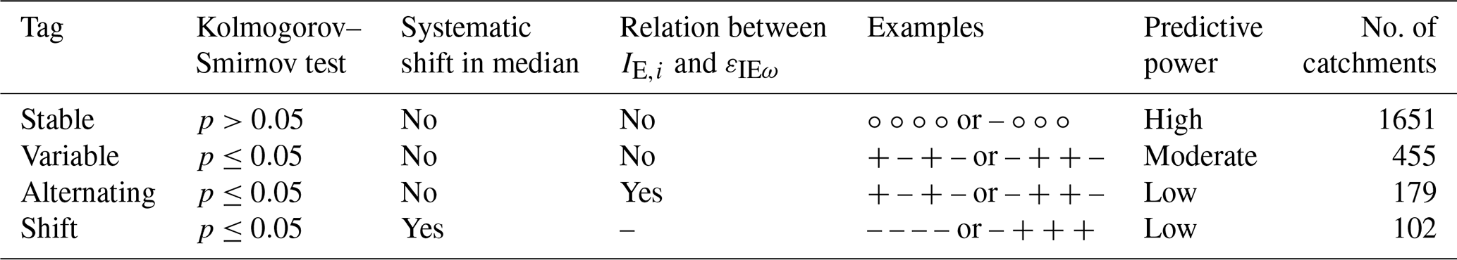
  Following the above, each catchment was classified into one of four qualitative categories of temporal stability of ε_IEω (Table 2). Note that the use of a formal quantitative statistical test was here hindered by the small sample size of a maximum of four pairs of time periods and thus omitted. The temporal stability was ranked as stable if between more than half of the j distributions in a catchment no significant differences in median ε_IEω values were found, e.g. ∘ ∘ ∘ ∘ or – ∘ ∘ ∘. A catchment was ranked as variable if it showed an alternating sequence and thus no systematic shift in median ε_IEω values over time, e.g. + – + – or – + + – and no relation between I_E,i and median ε_IEω. In contrast, if a catchment was characterized by an alternating sequence and a dependency between I_E,i and median ε_IEω, it was tagged as alternating. If, finally, between three or more of the j consecutive distributions in a catchment the median ε_IEω values were found to increase or decrease, e.g. – + + + or – – – –, this may indicate the presence of a systematic shift over time and the temporal stability of deviations from expected I_E was tagged as shift.

Table 2 Decision criteria to classify the time stability of the j distributions ε_IEΔj for each catchment into one of the four qualitative categories stable, variable, alternating, shift and the associated predictive power of the marginal distribution of ε_IEω values of a catchment, aggregating all j distributions of that catchment.

Step 5 – aggregated long-term marginal distribution of annual deviation ε_IEω values from expected I_E for each catchment.

In this step, the up to j=4 distributions ε_IEΔj were aggregated into one marginal distribution of ε_IEω values for each catchment (Fig. 3e). This distribution reflects the historical range of fluctuations in annual ε_IEω values based on all available information for each catchment. Consequently, the median ε_IEω of the distribution in each catchment represents a measure of uncertainty around expected future I_E based on current estimates of ω for each catchment, thereby making I_E statistically predictable.

To account for the potential effect of systematic shifts in distributions ε_IEΔj (Step 4) on the predictive power of the associated marginal distribution of deviation ε_IEω values, we tagged the marginal distribution of each catchment with a qualitative robustness flag as defined in Step 4. Stable distributions are characterized by the highest predictive power; distributions with variable fluctuations can be expected to have moderate predictive power, while distributions tagged as alternating or shift do, in the absence of more detailed data, have a rather low predictive power (Table 2).

Step 6 – evaluating the sensitivity of the marginal distributions of annual deviation ε_IEω values to the choice of 20-year averaging window.

To further quantify the sensitivity of the above aggregated, i.e. marginal distributions to the choice of the individual 20-year averaging time periods, we, in a last step, repeated the above Steps 1–5 twenty times to test all possible sequences of 20-year periods. More specifically, in a moving-window analysis, we first shifted each time period T₁–T₅ by 1 year, i.e. 1902–1921 (T₁), 1922–1941 (T₂), etc., and repeated the above Steps 1–5. Subsequently we shifted T₁–T₅ by another year to 1903–1922 (T₁), 1923–1942 (T₂), etc. and again repeated Steps 1–5. This was done 20 times until all years of the first period, i.e. 1901–1920, were the starting years of T₂.

3 Results

3.1 Changes in hydroclimatic variables and movement in Budyko space (Step 1)

Throughout the 100-year study period and across all study catchments, considerable hydroclimatic variability was observed, with some variables exhibiting trend-like behaviour over time and others more cyclic behaviour. Overall, mean annual precipitation over the individual 20-year periods systematically increased by ∼18.4 mm per century, on average (Fig. 4a), with 57 % of the catchments showing an increase between T₁ and T₂ (Δ₁₋₂) and 83 % for Δ₄₋₅. In contrast, mean annual temperatures (Fig. 4b) and the associated potential evaporation (Fig. 4c) were characterized by a more fluctuating pattern. These combined factors led to slightly more arid conditions in the first half of the 20th century, followed by a considerable reduction in aridity index I_A, and thus to a shift towards somewhat more humid conditions towards the end of the century across all of the temporal stability categories (Fig. 4e), in which, on average, 78 % and 75 % of the catchments showed decreases in I_A for Δ₃₋₄ and Δ₄₋₅, respectively. The changes in I_A were accompanied by related changes in potential evaporation (E_P) and precipitation (Fig. 4c and a). The overall movement of catchments in the Budyko space due to hydroclimatic changes is illustrated in Fig. S1 in the Supplement (Jaramillo and Destouni, 2014). If these movements were driven only by changes in I_A, catchments would be expected to move within the directional range of $\mathrm{45}<\mathit{\alpha }<\mathrm{90}\mathit{°}$ or $\mathrm{225}<\mathit{\alpha }<\mathrm{270}\mathit{°}$ (Jaramillo et al., 2022). However, observed movement of catchments is also found in other directions, indicating deviation (ε_IEω≠0) from the expected I_E, as elaborated in detail in Fig. S1.

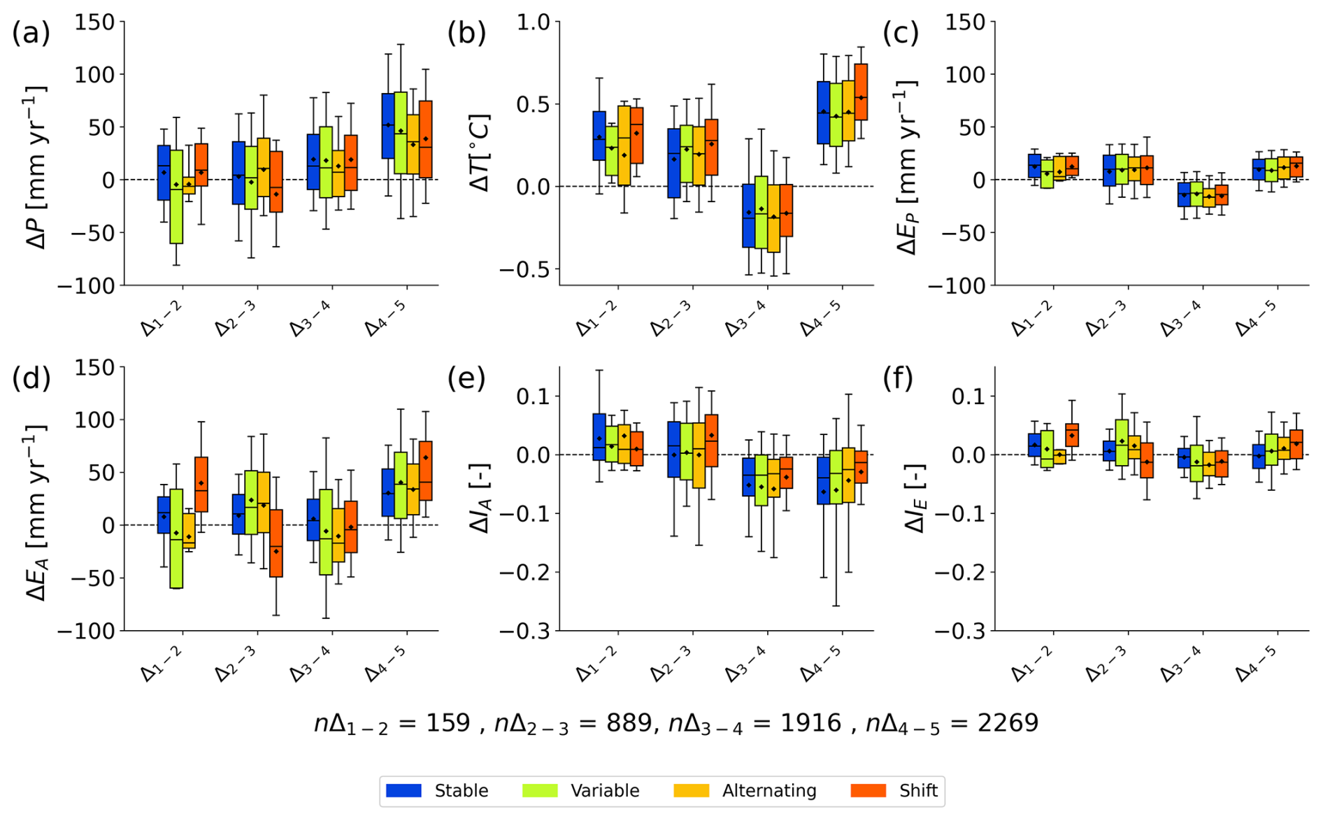
Figure 4 Temporal stability category-wise mean 20-year changes in hydroclimatic variables for the studied catchments between two consecutive periods. (a) Precipitation, P; (b) temperature, T; (c) potential evaporation, E_P; (d) actual evaporation, E_A; (e) aridity index, I_A; and (f) evaporative index I_E. The boxes represent the 25th to 75th percentiles, while whiskers extend to the 10th and 90th percentiles. Diamonds denote the arithmetic mean, and outliers are not shown.

It is worth mentioning here that the sample sizes vary between individual 20-year periods of comparison due to the length of the data availability. Therefore, to distinguish whether the climatic variability in Fig. 4 is associated with the hydroclimatic variables or is present due to the change in sample size, the same plot for the catchments that are present in all periods of comparison (n=142) is provided in Fig. S2 in the Supplement. It is found that the overall pattern of temporal variability in that sub-sample largely reflects that of the full sample.

3.2 Distributions of annual deviations ε_IEΔj from parametric Budyko curve (Steps 2 and 3)

The indicative evidence for the presence of deviation ε_IEω≠0 in at least some catchments is further supported by a more detailed analysis of the distributions of annual deviations ε_IEΔj between the pairs of subsequent 20-year periods for each of the 2387 study catchments. The results of the Wilcoxon signed rank tests indeed suggest that it is likely that the median ε_IEω≠0 for a significant proportion of catchments. For example, at a 95 % confidence level (i.e. p≤0.05), 34 %–42 % of the distributions can be considered to feature deviations with a median ε_IEω≠0 (Fig. 5a). Conversely, this also entails that for a majority of 58 %–66 % of the distributions there is less evidence (i.e. p>0.05) that the median ε_IEω is different from zero. Note that minor ε_IEω values were observed in most catchments. Although these ε_IEω values were not classified as significant based on the Wilcoxon signed rank test used here, it may be too naive to assume that the deviation ε_IEω values are strictly zero, as also demonstrated by Reaver et al. (2022). Overall, this is consistent with results from previous studies and shapes a picture in which catchments do not strictly and necessarily follow their expected parametric I_E curves, but that the deviations thereof remain close to zero or very limited for many catchments.

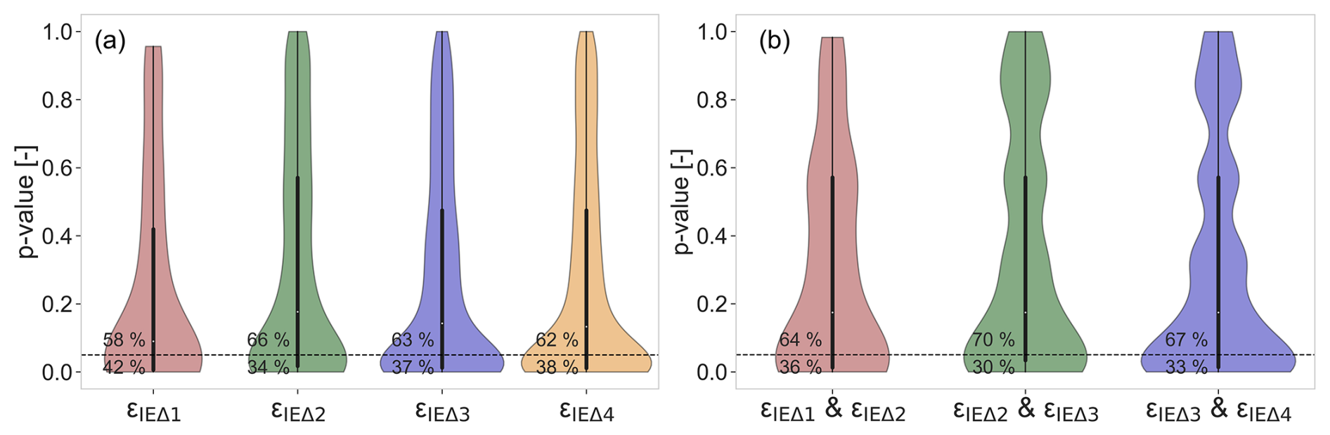
Figure 5 Distribution of p values from statistical tests. (a) Wilcoxon signed rank test performed to test whether the long-term median ε_IEω value of the individual 20-year distributions ε_IEΔj is significantly different from zero. The percentage above the significance line (0.05) shows data points where median ε_IEω values are not significantly different from zero, while the percentage below indicates those that are significantly different (b) Kolmogorov–Smirnov test performed on the distributions of two consecutive time periods (ε_IEΔj and ε_IEΔj+1) to test whether the two distributions of deviations are significantly different from each other. Here, the percentage above the significance line presents data points where the distributions of two consecutive time periods are not significantly different from each other, while the percentage below indicates significant differences. Each violin plot displays the distribution of p values, with the central black box representing the interquartile range (25th to 75th percentiles) and whiskers extending to the smallest and largest data points within 1.5 times the interquartile range. The dashed black line represents the significance level of 0.05.

A characteristic selected example for the latter is the sequence of the four distributions of annual deviations in the Chemung River at Chemung (New York; 6455 km²; ID US_0000832) across the four pairs of subsequent 20-year periods over the 20th century (Fig. 6a–c). The annual deviation ε_IEω values with an interquartile range of IQR∼0.062 (Fig. 6c) concentrate quite narrowly around the medians. The medians themselves range between merely ${\mathit{\epsilon }}_{\text{IE}\mathit{\omega }}=-\mathrm{0.006}$ and 0.012 (Fig. 6b). The associated p values from the Wilcoxon signed rank test (p=0.27–0.84) further suggest that there is only limited evidence that the median deviation ε_IEω values of distributions ε_IEΔj are different from zero. In spite of a somewhat wider spread with an IQR∼0.094 (Fig. 6f), a similar pattern with consistently low median, ${\mathit{\epsilon }}_{\text{IE}\mathit{\omega }}=-\mathrm{0.017}$–0.018 (Fig. 6e) (p=0.09–0.47), was observed in the second selected example, the Lee River (Ireland; 1019 km²; ID GB_0000078).

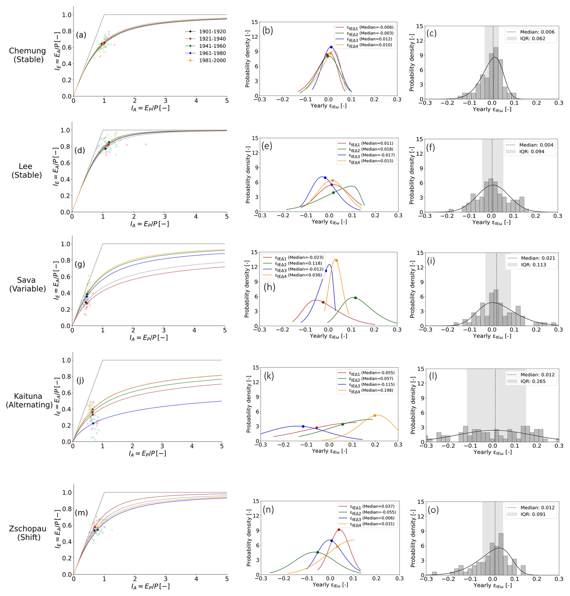
Figure 6 Mean annual position of catchments (faint dots) in Budyko space along with long-term mean (darker dots) and expected parametric Budyko curves (left column). Individual distribution of deviations (ε_IEΔ1, ε_IEΔ2, ε_IEΔ3, and ε_IEΔ4) with long-term median deviation ε_IEω values (middle column) and long-term marginal distribution of annual deviations along with long-term median values of ε_IEω and IQR of ε_IEω values (right column) for five example catchments: Chemung River (a–c), Lee River (d–f), Sava River (g–i), Kaituna River (j–l), and Zschopau River (m–o).

In contrast, more varied patterns were found for other catchments (Fig. 6g–o). For example, in the Sava River at Radeče (Slovenia; 6004 km²; ID SI_0000007), all four distributions of the annual deviations display a wider spread, with IQR∼0.113, indicating a higher degree of storage fluctuation between individual years (Fig. 6i). This variability may largely be attributed to hydropower developments and the associated changes in hydropower production levels (Levi et al., 2015), which disrupt natural flow regimes by increasing runoff during high demand and altering seasonal flow patterns (Renofalt et al., 2010; Lee et al., 2023). In addition, the medians do considerably deviate from zero, as indicated by median ε_IEω values ranging between −0.023 and 0.118 (Fig. 6h).

The set of 20-year average I_E values and the associated parameters of the fitted parametric distributions of deviations for each of the time periods in the individual study catchments are provided in the supplementary data downloadable from Zenodo (https://doi.org/10.5281/zenodo.14060926, Ibrahim et al., 2024).

3.3 Temporal stability of the distributions ε_IEΔj (Step 4)

Based on the Kolmogorov–Smirnov tests, it was found that overall 68 % of the distributions ε_IEΔj between consecutive pairs of time periods are not significantly different from each other (p>0.05; Fig. 5b). Following the criteria defined in Sect. 2.2, this resulted in 1651 catchments classified as stable (Table 2; Fig. 7a). For these catchments, together corresponding to ∼70 % of all 2387 study catchments, their respective marginal distribution of ε_IEω can thus be plausibly considered to have rather high predictive power. Example cases are the Chemung and Lee rivers (Fig. 6a–f), which are characterized by sequences ∘ ∘ ∘ ∘ and ∘ ∘ ∘ ∘, respectively.

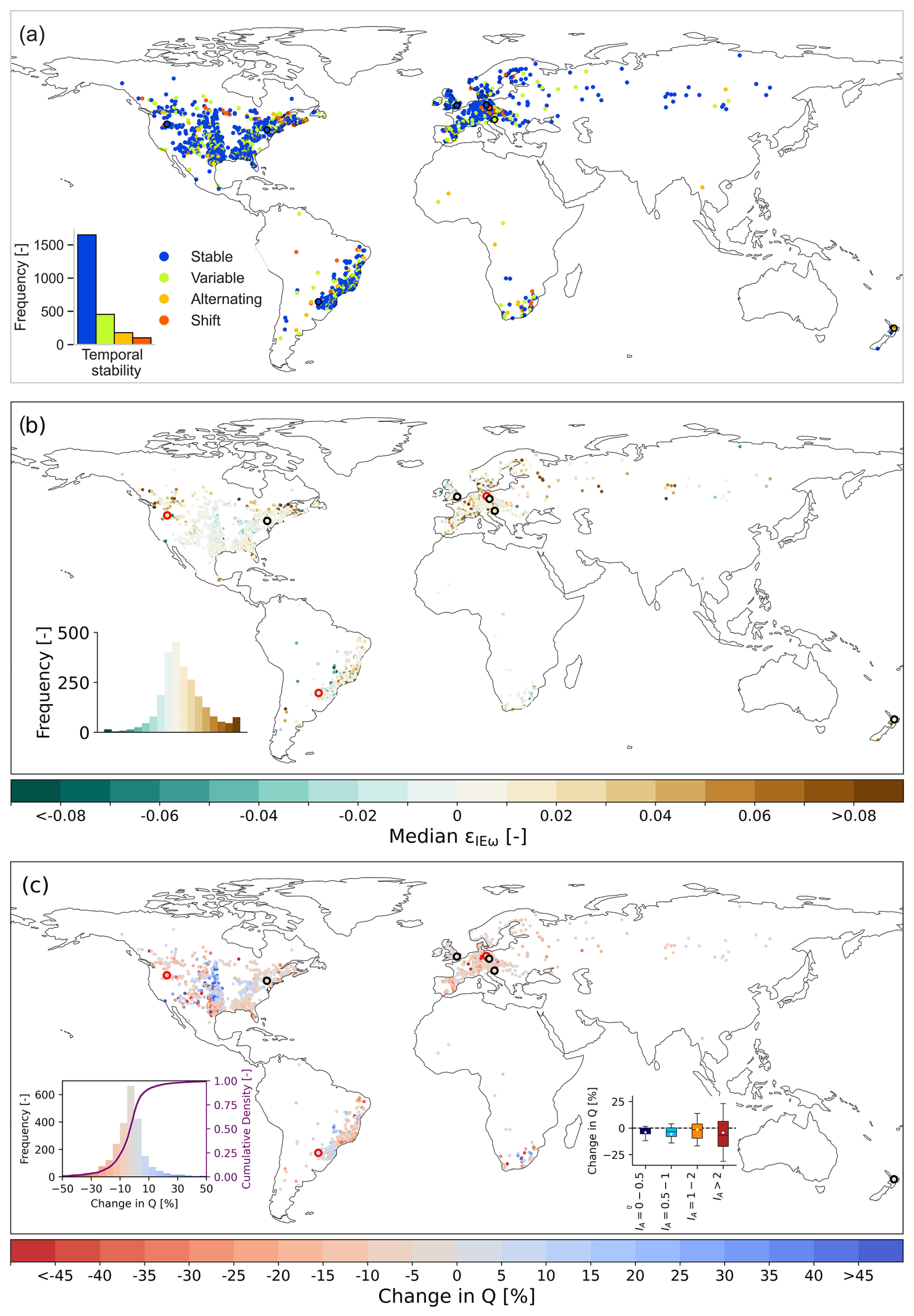
Figure 7 (a) Temporal stability and (b) long-term median ε_IEω value maps of aggregated long-term marginal distributions for the study catchments and (c) change in Q as a result of long-term median ε_IEω values. Histogram and cumulative density of change in Q and change in Q across different I_A bins are presented as two insets. Change in Q reflects the change due to median deviation ε_IEω values from the expected parametric Budyko curve only (i.e. excluding any change resulting from a change in aridity and its associated movement along the expected curve). Catchments highlighted with a black border represent the five selected examples from Fig. 6, while those outlined in red denote three additional selected example catchments shown in the Supplement (Fig. S5). The boxes represent the 25th to 75th percentiles, while whiskers extend to the 10th and 90th percentiles. Diamonds denote the arithmetic mean, and outliers are not shown.

Similarly, 455 additional catchments (19 % of all study catchments), whose distributions exhibited fluctuations over time (Kolmogorov–Smirnov test p≤0.05), but which featured only limited evidence for both the presence of systematic shifts over time and for a dependency between I_E,i and ε_IEω, were tagged as variable. An example of such a case is shown in Fig. 6g–i for the Sava River at Radeče (Slovenia; 6004 km²; ID SI_0000007). It can be seen that the distributions ε_IEΔj between the four pairs of time periods vary considerably, with medians ranging from −0.023 to 0.118. However, the fluctuations appear to occur alternatively (– + – +) and suggest neither the presence of a systematic shift over time (Fig. S4b in the Supplement) nor a dependency between I_E,i and median ε_IEω values (Fig. S4a). Despite these fluctuations, the marginal distribution of ε_IEω aggregated from the four individual distributions ε_IEΔj (Fig. 6i) can, although wider than for catchments tagged as stable, thus be assumed to be an at least moderately robust representation of ε_IEω.

In contrast, 7 % of the catchments were tagged as alternating, and a dependency between I_E,i and ε_IEω could not be ruled out. A characteristic example for this type of catchments is the Kaituna catchment (New Zealand; 706 km², ID NZ_0000003) in Fig. 6j–l. This catchment features major fluctuations, with median ε_IEω values between −0.115 and 0.198. In addition, although no systematic evolution of median ε_IEω over time was evident (Fig. S4d), the data suggest the potential presence of a dependency on I_E,i, as shown in Fig. S4c. The pronounced alternating behaviour of the ε_IEω, fluctuations between −0.115 and 0.198, could not be readily explained by factors such as land use changes as estimated from the Hilda+ gridded land cover product (Winkler et al., 2021), seasonality index (SI) of liquid precipitation input (i.e. rainfall + snowmelt), and Pardé coefficients or median rainfall intensity (Fig. S3a, c, e, and f in the Supplement). The SI was calculated using the formula proposed by Gao et al. (2014). A higher SI value indicates that most of the precipitation falls within a few months, while a lower value reflects more evenly distributed precipitation throughout the year. This suggests that other additional drivers, or a combination of drivers, influence this catchment's alternating behaviour.

The remaining 102 catchments (4 %) were tagged as shift as they exhibit a rather consistent shift in median ε_IEω over time. This can be seen for a selected example in Fig. 6m–o. The median ε_IEω in this catchment of the Zschopau River (Germany; 1544 km²; ID DE_0000027) does not only significantly vary between −0.055 and 0.037, but it does so rather systematically into one dominant direction after ε_IEΔ1 (+ – + +; Fig. 6n). This shift aligns with a gradual decrease in the 20-year seasonality index (SI) (Fig. S3e) of liquid precipitation input (i.e. rainfall + snowmelt). In the Zschopau River catchment, this decrease in SI towards the end of the century signifies a shift towards a more evenly distributed precipitation pattern. These changes coincide with an increase in forest cover towards the end of century, as estimated from Hilda+ data (Fig. S3b). Additionally, Renner et al. (2014) and Renner and Hauffe (2024) reported a gradual recovery of forests in the Zschopau catchment during this period, which may further contribute to the observed shift.

As can be seen in Fig. 7a, the time stability of the studied catchments is geographically rather homogenously distributed. Catchments tagged as stable and variable can be found globally, while also no regional concentrations of catchments tagged as alternating and shift could be identified.

3.4 Aggregated long-term marginal distribution of annual deviation ε_IEω values (Step 5)

By aggregating its j individual distributions, a long-term marginal distribution of ε_IEω for each catchment was built. For a large majority of catchments, the long-term median ε_IEω value remains very close to zero. More specifically, ∼50 % of all study catchments are characterized by a median deviation ε_IEω value that does not exceed ±0.015 and ∼70 % by a median within the interval ±0.025 (Fig. 8a). Depending on the time stability of the j individual distributions in a catchment, the spread of annual deviations around these medians showed a more variable pattern. Overall, for >50 % of the study catchments, the IQR of annual deviations remained below 0.08 and for ∼70 % below 0.10 (Fig. 8b). While catchments with stable distributions exhibit, in general, a rather narrow spread with an average IQR∼0.08, catchments with distributions tagged as variable feature a bit of a wider spread with an average IQR∼0.10 while still centring closely around zero. This can also clearly be seen by the selected examples in Fig. 6. The medians of the marginal distributions of the Chemung and Lee rivers, both tagged as stable, are ∼0.006 and ∼0.004 respectively, with narrow IQRs of 0.062 and 0.094 (Fig. 6c and f). In contrast, while also featuring a marginal distribution with a median deviation ε_IEω∼0.021, the Sava River catchment (Fig. 6i), tagged as variable, is characterized by a considerably wider scatter of the annual deviations around the median as evident in the higher IQR of ∼0.113. Three additional illustrative examples of well-known river basins are presented in Fig. S5 in the Supplement. In contrast, the analysis, which uses the earliest available period as a fixed baseline, shows an increase in the number of stable catchments along with a slightly higher median ε_IEω values. Further details are provided in the Supplement (Fig. S6a–f).

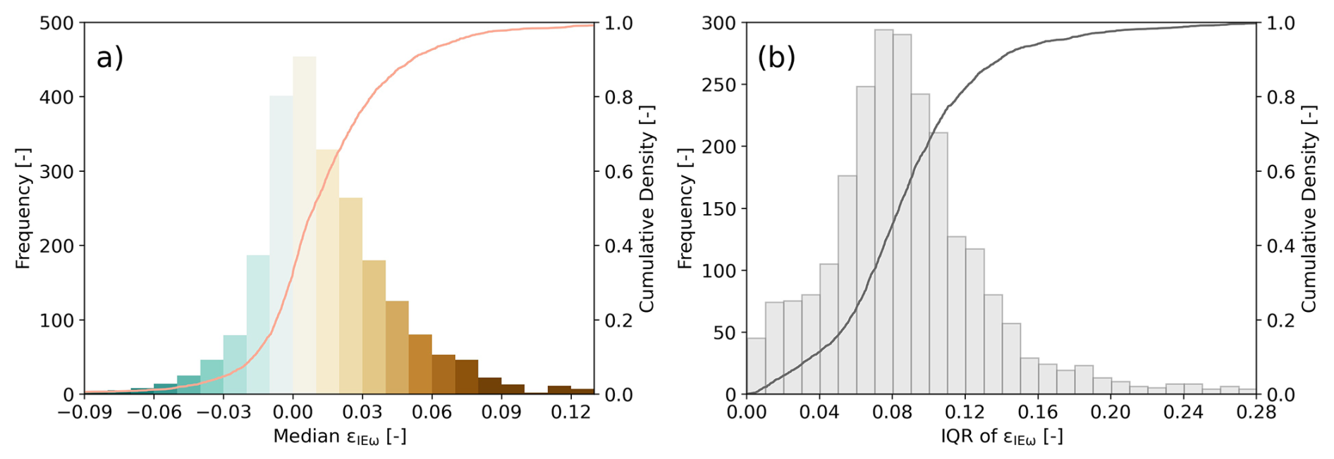
Figure 8 Visualization of long-term (a) median ε_IEω and (b) interquartile range (IQR) of ε_IEω for aggregated long-term marginal distribution of ε_IEω across all catchments (2387) along with the corresponding cumulative distribution function (CDF). The varying colour palette in Fig. 8a aligns with the palette used in Fig. 7b to maintain consistency. In Fig. 8b, a uniform colour is used since IQR values are all positive.

Overall, it can be observed that median deviation ε_IEω values close to zero are dominant globally, with no obvious spatial clustering of more pronounced deviations (Fig. 7b). However, it can also be seen that there is some geographic grouping in the direction, i.e. the sign, of the median ε_IEω. While for many catchments in the central US and southern Brazil median deviations are negative, i.e. ε_IEω<0, the rest of the study catchments globally are dominated by ε_IEω>0. Overall, median deviations from the expected parametric Budyko curve resulted in regionally distinct relative changes in Q across the studied catchments, with around ∼68 % of the catchments exhibiting changes (ΔQ) of less than ±10 % (Fig. 7c). However, catchments in some regions, notably in the central US and southern Africa, can be characterized by ΔQ exceeding ±25 %. Overall, the results indicate that catchments in more arid regions (I_A>2) are particularly susceptible to relative changes in discharge as compared to more humid regions (inset Fig. 7c).

For a more regional evaluation, the yearly ε_IEω values for individual catchments were aggregated into regional marginal distributions of ε_IEω stratified according to the long-term mean aridity index (I_A) and varied latitude bands (Fig. 9a). These regional distributions capture the variability in yearly ε_IEω across regions, with the median ε_IEω serving as a robust measure of central tendency. The general pattern found across most regions with available data is broadly consistent. Overall, 16 out of 20 regions are characterized by median deviation ε_IEω values that do not exceed ±0.02. Similarly, no consistent directional pattern in the magnitude of regional median ε_IEω could be identified either (Fig. 9b). For higher latitude regions beyond ±30°, the minor fluctuations in median ε_IEω bear no evidence for a relationship with I_A. On the other hand, the data suggest that the spread around the regional medians consistently decreases with increasing I_A across all latitude bands except the 50–90° N band, as shown by the sequence of IQR in Fig. 9c. This indicates that catchments in more humid regions across the study domain are subject to more pronounced annual water storage fluctuations.

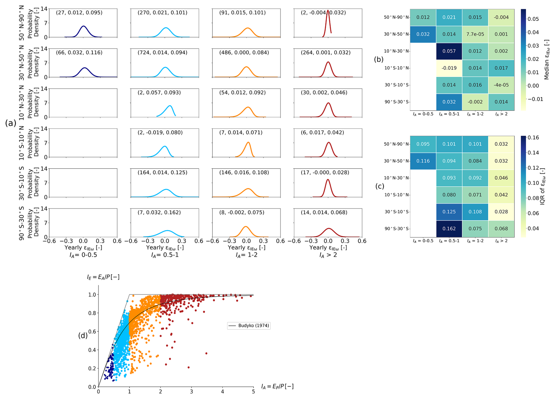
Figure 9 (a) Regional marginal distributions of ε_IEω for defined latitude and I_A bins. The three numerical values in small brackets at the top of each panel presents number of catchments in that category, long-term median ε_IEω, and IQR value of ε_IEω, respectively. (b, c) Variation in median and IQR values of ε_IEω for the regional marginal distribution of ε_IEω. (d) Long-term position (1901–2015) of catchments in Budyko space. The colour of the dots corresponds to the regional marginal distributions of ε_IEω for the corresponding I_A bin.

The parameters of the fitted parametric regional and catchment-specific marginal distributions together with the associated predictive robustness flags, as defined by the time stability of the j individual distributions for each catchment, are provided in Ibrahim et al. (2024, https://doi.org/10.5281/zenodo.14060926) and can be used, depending on their robustness flag, to estimate $I_{\mathrm{E},t}=I_{\mathrm{E},i}+{\mathit{\epsilon }}_{\text{IE}\mathit{\omega }}$ for a catchment under future hydroclimatic conditions.

3.5 Sensitivity of marginal distributions of deviation ε_IEω values to the choice of 20-year averaging window (Step 6)

The moving-window analysis to quantify the sensitivity of the marginal distributions of ε_IEω resulted in 20 individual, yet not uncorrelated, marginal distributions for each study catchment. Through this approach, we observed that the aggregated marginal distributions of ε_IEω may indeed be subject to differences. The magnitudes of the fluctuations vary between catchments but remain in general rather minor.

The Chemung and Lee rivers are two examples for a very low sensitivity of the marginal distributions of ε_IEω to the choice of time periods. The differences between the medians of the two most extreme marginal distributions does not exceed ∼0.008 for the Chemung (Fig. 10a), and 90 % of the medians of the 20 marginal distributions fall within an interval of merely 0.01. In addition, the distributions maintain comparable shapes. Similar behaviour was observed for the Lee River (Fig. 10b), with the medians of the two most extreme distributions differing only by ∼0.014. In this case, 75 % of the medians are observed within an interval of 0.01.

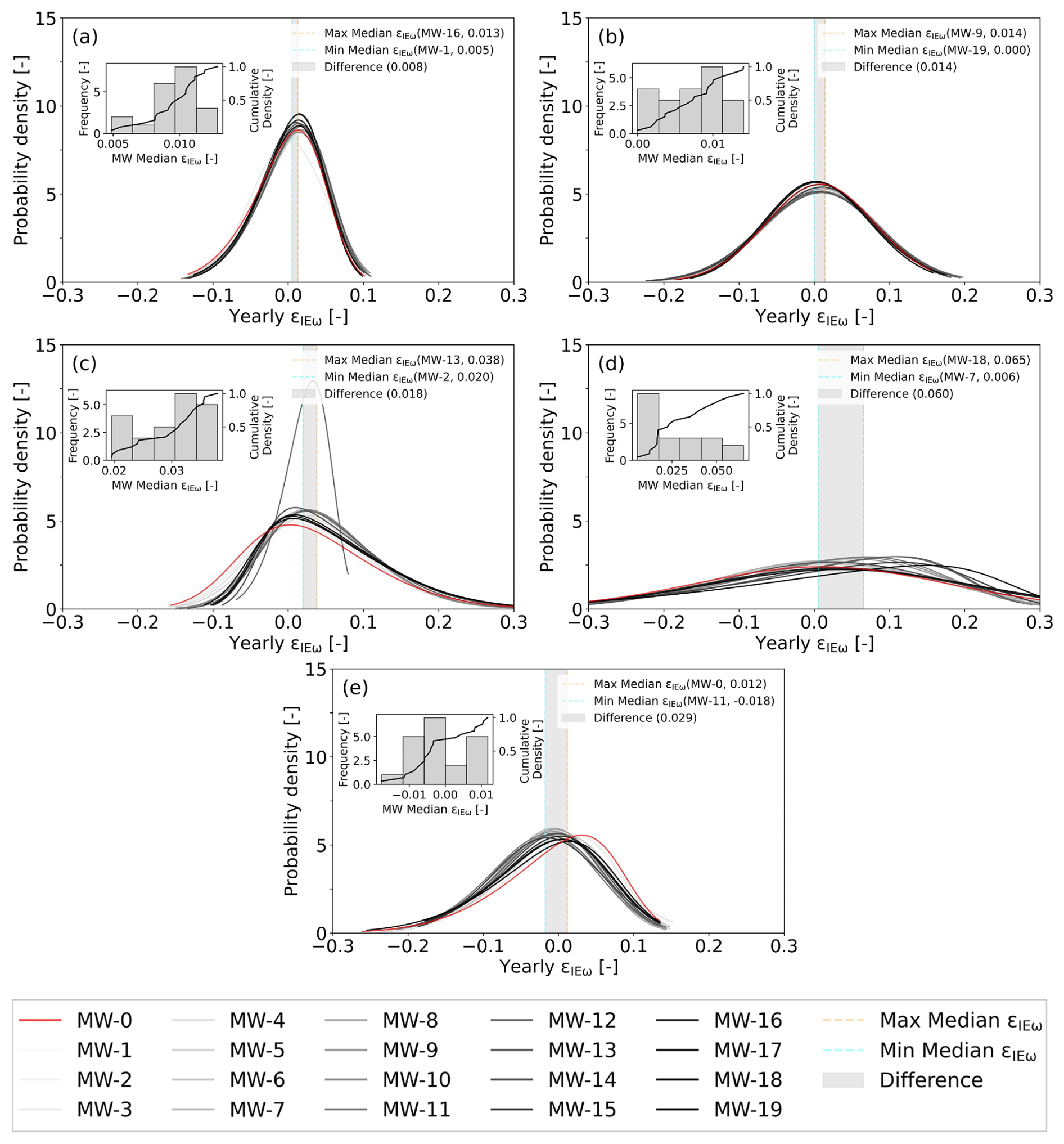
Figure 10 Aggregated marginal distributions of ε_IEω for 20 moving-window time periods for five example catchments: (a) Chemung River, (b) Lee River, (c) Sava River, (d) Kaituna River, and (e) Zschopau River. The red line represents the original marginal distribution of ε_IEω. The orange and aqua-coloured dashed lines depict the maximum and minimum median ε_IEω values corresponding to their respective moving-window time periods. The grey shaded area visually portrays the difference between the extreme maximum and minimum median ε_IEω values across the moving-window time periods.

However, in the case of catchments that are tagged as variable, alternating, or shift, the difference in medians of the two extreme marginal distributions is observed to be increased. For the Sava River catchment (Fig. 10c), tagged as variable, the difference between the two extreme marginal distributions is ∼0.018, with 75 % of the medians within an interval of 0.032. For Kaituna River (Fig. 10d), tagged as alternating, the difference between the medians of the two extreme marginal distributions is quite large, with a value of 0.060. For 15 out of the 20 marginal distributions, the medians are found to fall within the range of 0.046. A similar pattern for Zschopau River (Fig. 10e), tagged as shift, is observed with a median difference for two extreme marginal distributions to be 0.029.

Overall, it was found that for 78 % of the study catchments in 15 out of 20 time windows, i.e. 75 %, feature median deviation ε_IEω values within an interval of ±0.035. This further suggests that, although some sensitivity to the choice of time period can occur, the magnitude of the fluctuations remains rather minor for a large majority of catchments.

Similarly, the distribution of the median ε_IEω of all study catchments, e.g. Fig. 7b, remains rather stable when evaluated over the 20 subsequent moving windows, as shown in Fig. 11, with neither the medians nor the spread of the distributions experiencing marked variations. Although lumping the medians of all catchments into one distribution may conceal fluctuations between moving windows of individual catchments, it nevertheless allows for the observation that there is no systematic larger-scale effect.

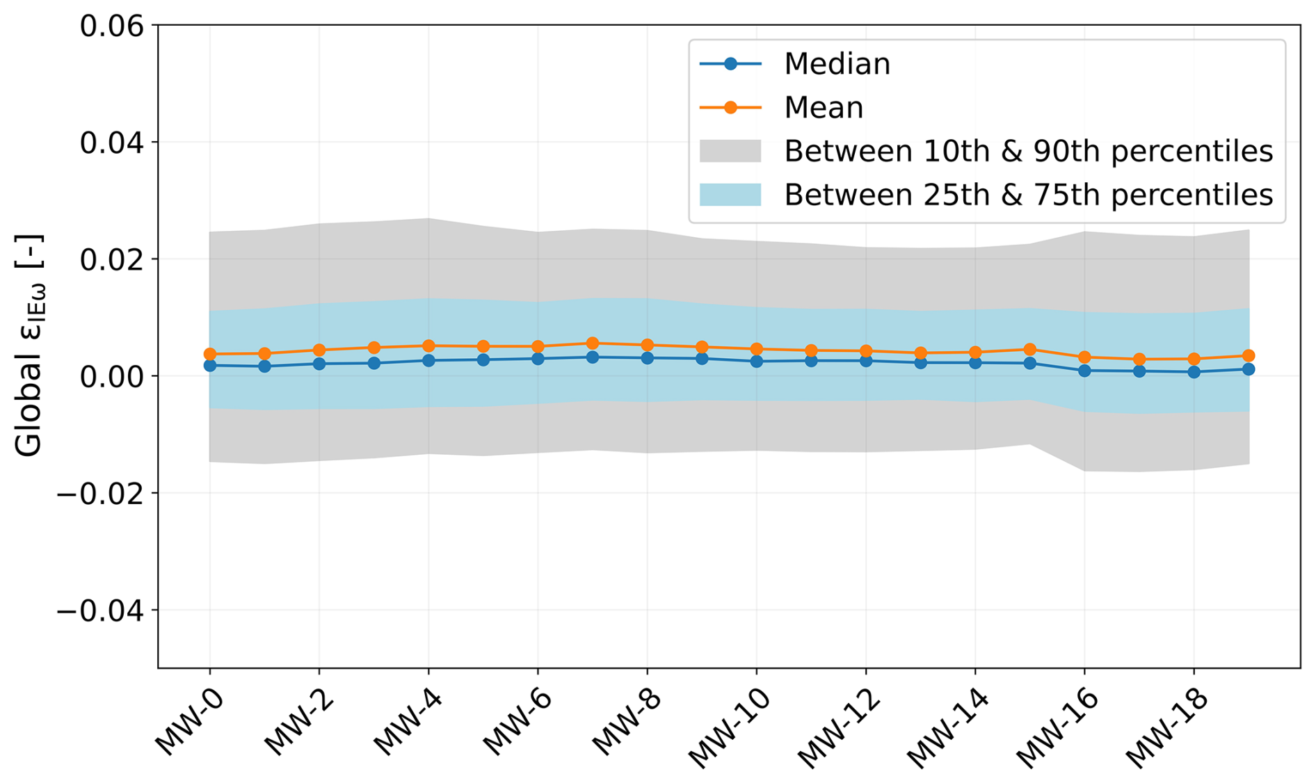
Figure 11 Variation in global long-term median, mean, 10th and 90th percentiles, and 25th and 75th percentiles of ε_IEω for all of the catchments with respect to each moving window.

4 Discussion

Our analysis revealed that most study catchments underwent continuous multi-decadal hydroclimatic fluctuations throughout the 20th century (Figs. 4 and S1). Notably, these fluctuations were largely consistent across the different temporal stability categories. Unlike previous studies comparing only two time periods (Jaramillo and Destouni, 2014), here the higher temporal resolution, with up to five 20-year periods, showed that these fluctuations were not one-directional, with the first half of the century trending towards higher aridity and the latter half towards increased humidity, suggesting cyclic behaviour rather than trends over longer timescales.

In alignment with previous studies (Berghuijs and Woods, 2016; Jaramillo et al., 2018, 2022; Reaver et al., 2022), our analysis suggests that following disturbances and thus changes in I_A, catchments do not necessarily and strictly follow their specific parametric Budyko curves as defined by parameter ω. In our analysis, we found that the general magnitudes of the median deviation ε_IEω values across all study catchments throughout the 20th century are very minor, with median ${\mathit{\epsilon }}_{\text{IE}\mathit{\omega }}\le \pm \mathrm{0.015}$ for 50 % and $\le \pm \mathrm{0.025}$ for 70 % of the catchments. This corresponds well with the results of Jaramillo and Destouni (2014) and Jaramillo et al. (2018), who estimated absolute mean deviations from the expected I_E of ε_IEω∼0.01–0.02 over two multi-decade periods, for different regions in the world, based on an analysis of several hundred catchments.

Based on annual water balance data of ∼400 catchments in the United States, Berghuijs and Woods (2016) reported an average difference of around 28 % between the spatial and temporal sensitivity of I_E to changes in I_A. However, a back-of-the-envelope calculation assuming an average ω=2.6 (Greve et al., 2015) suggests that even with a pronounced shift in aridity of ΔI_A=0.2 (Jaramillo and Destouni, 2014), such a difference (28 %) in sensitivity leads to only minor absolute deviations from the expected I_E with ε_IEω∼0.01–0.04 (4 %–8 %) for regions with the most common I_A=0.5–2.5, which broadly corresponds to the results of our study. In contrast, Reaver et al. (2022), using data from ∼700 catchments from the CAMELS-US (Newman et al., 2015) and the CAMELS-UK datasets (Addor et al., 2017; Coxon et al., 2020), provided a detailed and exhaustive analysis of possible temporal trajectories through the Budyko space over several decades. They report the mean of all study catchments' maximum relative deviations of the actually observed, empirical values of I_E,o from the predicted values of I_E by catchment-specific curves, with ${\mathit{\epsilon }}_{\text{IE}\mathit{\omega },\text{max}}=I_{\text{E,o,max}}-I_{\text{E,max}}\sim \mathrm{26}$ %. However, that mean value of all catchment maxima is strongly biased by a few rather extreme outliers in their analysis, and the vast majority of their study catchments (>650 out of 728) exhibits much lower errors, with a median maximum deviation of ${\mathit{\epsilon }}_{\text{IE}\mathit{\omega },\text{max}}\sim \mathrm{9}$ % (see Fig. 3 in Reaver et al., 2022). It may thus prove more informative to interpret the results of Reaver et al. (2022) based on the mean instead of the maximum deviations as these average conditions do almost certainly occur more frequently. By doing so, it is plausible to assume that the deviation ε_IEω values will be considerably lower than the maximum ${\mathit{\epsilon }}_{\text{IE}\mathit{\omega },\text{max}}\sim \mathrm{9}$ % and potentially closer to the range of 4 %–8 % estimated above and thus overall consistent with the results of our analysis.

However, we also note that these minor deviations may have different practical implications in different climates (Fig. 7c). For example, in a humid catchment with I_A=0.5 (e.g. mean annual P=2000 mm yr⁻¹, E_P=1000 mm yr⁻¹ and Q=1120 mm yr⁻¹), a deviation of ε_IEω=0.02 results in ΔQ∼40 mm yr⁻¹, equivalent to merely 3 % of water yield, which hardly affects water supply. In contrast, the practical effects are more pronounced in arid environments. In a typical catchment with I_A=2 (e.g. P=500 mm yr⁻¹, E_P=1000 mm yr⁻¹, Q=60 mm yr⁻¹), the same deviation will lead to a ΔQ∼10 mm yr⁻¹, equivalent to ∼15 % of the available water yield, and thus have considerable higher relevance for water resources planning. For such environments, a robust quantification of expected deviations may thus prove beneficial for future estimates of water resources availability.

Despite some spatial clustering, the deviation ε_IEω values from the expected parametric Budyko curves do not exhibit any clear and unambiguous relationships with several climatic variables (Fig. S7 in the Supplement). The detailed processes and reasons underlying the deviations thus remain so far unknown and may be assumed to be manifold and to vary depending on the characteristics of specific sites. In any case, it is plausible to assume that the reasons are a combination of factors, including, amongst others, changes in precipitation volumes, seasonality, and phase; changes in atmospheric water demand; changes in land cover; human interventions, such as reservoir operation or irrigation; and also violations of the assumption that $\mathrm{d}S/\mathrm{d}t\sim \mathrm{0}$ over the 20-year time periods (Han et al., 2020) and other uncertainties in the available data (Beven, 2016). Note that a detailed exploration of this issue is beyond the scope of this paper.

To our knowledge, this is the first study to quantify the evolution of median ε_IEω over multiple time periods. This allowed us to build distributions to predict future ε_IEω based on historic data, together with an indicative robustness flag, describing their temporal stability and thus their suitability to predict ε_IEω under future hydroclimatic conditions. It was found that, globally, median ε_IEω does not only remain minor but, perhaps even more importantly, also rather stable over time. For ∼70 % of the study catchments, the annual distributions of ε_IEω, and thus also their 20-year medians, were classified as stable. In other words, the available data suggest that over multiple 20-year periods in the past century, the samples of annual deviations originate from the same distribution. This further allows for some confidence to plausibly assume that ε_IEω and the associated I_E under projected future hydroclimatic conditions can, at least for several decades, be robustly predicted based on these distributions. However, it is important to note that the 20-year time periods used in this study, while effective for medium-term projections, may limit the ability to make long-term climate projections.

Further 19 % of catchments were classified as variable because their distributions of annual deviations for the individual 20-year periods exhibit some variability. Despite this, there is no indicative evidence to link this variability to alternating fluctuations or systematic, one-directional shifts and thus to quantifiable deterministic processes. In this case, the fluctuations can be assumed to be arbitrarily variable, allowing for the aggregation of a marginal distribution that reflects all available past knowledge. Although the uncertainty of that distribution may often exceed that of stable catchments, resulting in somewhat lower predictive power (Montanari and Koutsoyiannis, 2014), it is reasonable to assume that ε_IEω remains predictable. The fitted parametric marginal distributions of catchments tagged as stable and variable can be directly used to sample distributions of future annual ε_IEω and to estimate the average ε_IEω for that future period from the expected future I_E based on ω of the past 20-year period.

For catchments tagged as alternating or shift, the above assumption may be too optimistic. Although the sample size characterizing the evolution of ε_IEω over the study period is, with a maximum of j=4 pairs of 20-year periods, very small and thus no meaningful formal statistical tests could be executed, the data do not rule out the possibility that ε_IEω in these catchments is characterized by alternating or shift-like behaviours. In other words, ε_IEω may not be sampled from different distributions that change arbitrarily over time but from distributions that (here) either depend on I_E of the preceding time period or systematically increase or decrease over time. In these cases, the aggregated marginal distribution may produce spurious predictions of ε_IEω.

For catchments tagged as alternating, the user may instead want to consider constructing and using a conditional distribution in the form of ε_IE|ωi, i.e. a distribution of ε_IEω given the position I_E,i, for more reliable estimates. However, note that the limited data available for a maximum of four pairs of time periods poses a practical complication to construct a meaningful conditional distribution ε_IE|ωi, which is necessary to infer ε_IE|ωi. Alternatively, the user can decide to base predictions only on basis of the ε_IEω distribution of the last available time period to avoid the use of the marginal distribution (Montanari and Koutsoyiannis, 2014). For predictions in catchments with a suspected presence of a systematic shift, tagged as shift, users may choose to extrapolate the fitted distribution parameters of the individual pairs of periods to account for their shifts over time. However, here the reliability of this will depend on the strength of the individual relationship over the past and needs to be evaluated on a case-to-case basis as both categories are likely to lead to rather unreliable future estimates.

In any case, empirical models like the Budyko framework have inherent weakness in dealing with previously unseen changes in the underlying distribution of a specific variable (here ε_IEω). Our classification of catchments into stable, variable, alternating, and shift categories aims to capture varying levels of sensitivity to changes in underlying distributions. Catchments classified as alternating or shift are more likely to have experienced large changes in the underlying distributions and may thus remain sensitive to future changes, making empirical models less robust for predictions in these cases. Conversely, stable and variable catchments exhibited much less sensitivity to past climatic variability. In the absence of statistical evidence for changing distributions, it is reasonable to assume that they remain relatively insensitive to change in the near future, allowing empirical models to provide plausible predictions.

It is important to note that approximately 89 % of the study catchments are either stable or variable, with only a small minority (∼11 %) exhibiting alternating or shift behaviour. This predominance of stable or variable catchments supports the broad applicability of the Budyko framework for predictive purposes. Although there is no clear spatial pattern, the regional distributions of ε_IEω remain, with medians of ∼0–0.02 (Fig. 9a), broadly consistent with the global distribution (Fig. 8a) but also with each other across most spatial and climatic classes. This indeed suggests that the overall pattern is rather homogenous and regional effects remain limited, making probabilistic predictions feasible in the absence of a deterministic description (Montanari and Koutsoyiannis, 2014). Thus, the presented distributions (Figs. 8a and 9a) are in the absence of further information useful to quantitatively estimate the uncertainty for any specific catchment based on past information in a probabilistic way. However, caution is advised for out-of-sample catchments, where the assumption of stationarity may lead to less reliable predictions as the framework cannot take into account systematic shifts or alternating behaviour.

Despite the challenges associated with catchments classified as alternating and shift, the Budyko framework remains useful for identifying human-driven changes to the water cycle. Although many catchments showed only minor deviations, these deviations are key for recognizing drivers of change. Categorizing catchments into stable, variable, alternating, and shift can guide targeted future research. For example, catchments in the alternating and shift categories my either have been, in the past, subject to more substantial human interference than those in the other categories or be more sensitive to human-induced changes. Further investigations into the drivers of these deviations may strengthen our understanding of how human-induced changes influence catchment responses differently in different environments.

It was further found that the choice of a specific 20-year window can indeed lead to fluctuations in the distributions of ε_IEω. However, the magnitude of these fluctuations remains rather limited for the vast majority of catchments. To avoid misinterpretations, we have therefore added the IQR of median ε_IEω from the 20 individual moving windows as an additional robustness flag for each catchment in Supplementary data downloadable from a Zenodo repository (https://doi.org/10.5281/zenodo.14060926, Ibrahim et al., 2024). Lower IQR then indicates lower sensitivity to the choice of the 20-year window and thus a higher robustness of the marginal distribution for predictions of ε_IEω under future conditions.

A complete list of the parameters and robustness flags of the individual 20-year distributions as well as of the local aggregated marginal distributions with associated changes in Q for each of the 2387 study catchments, but also of the regional distributions as stratified by latitude and I_A, is provided in Ibrahim et al. (2024, https://doi.org/10.5281/zenodo.14060926). These distributions of annual ε_IEω can be directly used to predict the median ε_IEω under future conditions locally in these catchments or regionally by sampling over 20 projected future years.

5 Conclusions

Based on up to 100 years of hydroclimatic and streamflow data for 2387 river catchments worldwide, we test here whether catchments follow their specific parametric Budyko curves as defined by parameter ω over multiple 20-year periods throughout the 20th century.

The main findings of our analysis are as follows:

1. Overall, 62 % of the catchments do not significantly deviate from their expected parametric Budyko curves, although minor deviations were still observed. However, this also entails that a fraction of 38 % does indeed deviate.

2. The overall magnitude of deviations is minor. For ∼70 % of the catchments, the median deviations do not exceed ${\mathit{\epsilon }}_{\text{IE}\mathit{\omega }}=\pm \mathrm{0.025}$, which is equivalent to ∼1 %–4 %, depending on I_E. These median ε_IEω values, when expressed as relative changes in Q, result in less than a ±10 % change in discharge for most catchments.

3. For 89 % of the study catchments, ε_IEω can be considered highly or at least moderately well predictable based on historical data as distributions of ε_IEω in the past were shown to be stable over multiple time periods or characterized by variable fluctuations. The framework works well for most catchments; however, for out-of-sample catchments showing systematic shifts or alternating behaviour, additional analysis may be required.

The above implies that while catchments indeed may not strictly follow their parametric Budyko curves, as defined by parameter ω, the deviations remain in general minor and predictable. The latter is of particular importance for catchments in water-limited regions, where already small deviations can considerably affect available water supply and where robust predictions of these deviations are instrumental for effective future water resources planning and management.