Feature scale and identifiability: how much information do point hydraulic measurements provide about heterogeneous head and conductivity fields?

We systematically investigate how the spacing and type of point measurements impact the scale of subsurface features that can be identified by groundwater flow model calibration. To this end, we consider the optimal inference of spatially heterogeneous hydraulic conductivity and head fields based on three kinds of point measurements that may be available at monitoring wells, namely head, permeability, and groundwater speed. We develop a general, zonation-free technique for Monte Carlo (MC) study of field recovery problems, based on Karhunen–Loève (K–L) expansions of the unknown fields whose coefficients are recovered by an analytical, continuous adjoint-state technique. This technique allows for unbiased sampling from the space of all possible fields with a given correlation structure and efficient, automated gradient-descent calibration. The K–L basis functions have a straightforward notion of wavelength, revealing the relationship between feature scale and reconstruction fidelity, and they have an a priori known spectrum, allowing for a non-subjective regularization term to be defined. We perform automated MC calibration on over 1100 conductivity–head field pairs, employing a variety of point measurement geometries and evaluating the mean-squared field reconstruction accuracy, both globally and as a function of feature scale. We present heuristics for feature-scale identification, examine global reconstruction error, and explore the value added by both the groundwater speed measurements and by two different types of regularization. We find that significant feature identification becomes possible as feature scale exceeds 4 times the measurement spacing, and identification reliability subsequently improves in a power-law fashion with increasing feature scale.

1 Introduction

In the following, we quantify the reliability of reconstruction of heterogeneous hydraulic conductivity field features – meaning regions of locally similar hydraulic conductivity – of different scales, given different densities and kinds of point hydraulic measurements. We study a basic question that is inherent in all remote sensing: how much information can be extracted and at what resolution? A rigorous feature-scale perspective, which we have not seen before in the context of the inverse problem of hydrogeology, is illuminating, because model calibration may succeed in capturing large-scale features of hydrogeological relevance, while the L² (integral square) error of the recovered field relative to the true field remains misleadingly high. In the middle column of Fig. 1, we show two log-conductivity fields that have been reconstructed using gradient-descent model calibration. While both reconstructed fields qualitatively match the true field, in both cases calibration was able to remove only $\mathrm{2}/\mathrm{3}$ of the L² error relative to the underlying field. However, the remaining error pertains to higher wavenumber (i.e., spatial frequency) features which may be of less importance.

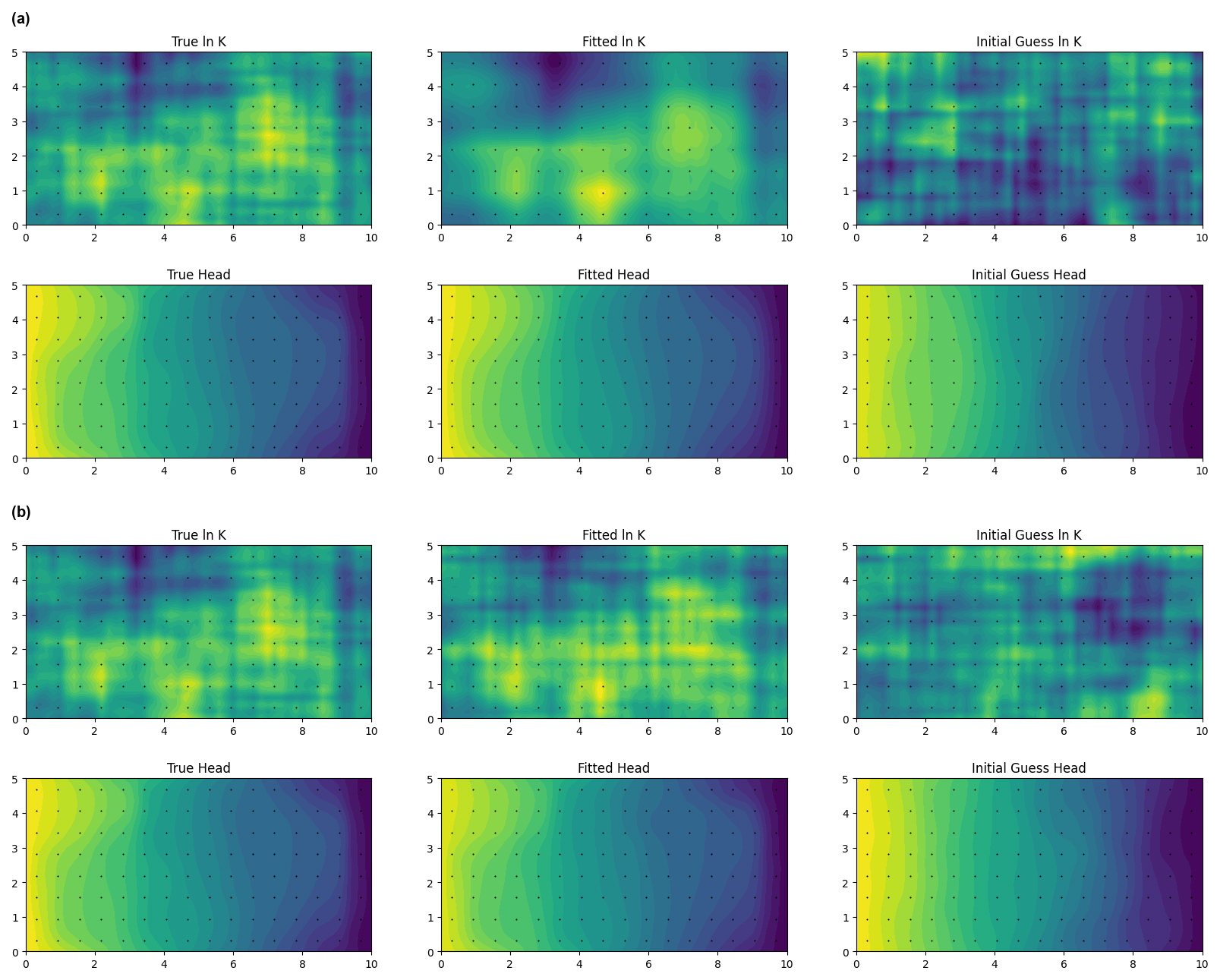
Figure 1 Examples of automated calibration (center column) of true fields $\ln \stackrel{\mathrm{̃}}{K}$ and $\stackrel{\mathrm{̃}}{h}$ (left column) after 500 optimization steps starting from an initially uncorrelated ln K field (right column), using the adjoint-state approach detailed in this paper. Color maps represent spatial variation of field values: a higher value corresponds to a lighter color within a given map, but numeric interpretation of a given color varies from map to map. Black dots in each image indicate the locations of simulated measurements. Two calibrations are shown, both featuring the same underlying field and the same data weights, as defined in Eqs. (37)–(39), but differing in regularization approach: (a) regularization employed with w_R = $\mathrm{1}/\mathrm{2}$ and (b) no regularization (w_R = 0). Ψ = 0.10 in both cases.

1.1 Detailed motivation

For many forms of groundwater modeling, it is common to infer the spatially heterogeneous hydraulic conductivity and head fields which together determine groundwater flow from sparse, passively collected measurements at groundwater wells. While significant high-resolution information about heterogeneity may be obtained from a wide variety of interventions including geophysical measurements (Slater, 2007; Szabó, 2015), hydraulic tomography (Illman et al., 2007), and both push–pull (Hansen et al., 2017) and point-to-point (Irving and Singha, 2010) tracer tests, such data are often unavailable at scales of interest. Due to their prevalence in practical, field-scale model calibration, we focus here on three types of point information that are readily and commonly determined at monitoring wells. These are hydraulic head, $\stackrel{\mathrm{̃}}{h}$, obtained from direct piezometry; Darcy flux magnitude, $\stackrel{\mathrm{̃}}{q}$, obtained from point dilution tests; and log of hydraulic conductivity, $\ln \stackrel{\mathrm{̃}}{K}$, from slug tests or Kozeny–Carman core sample analyses. Calibrating a spatially nonuniform hydraulic conductivity field at high resolution from sparse measurements of these three types is generally a highly underdetermined inverse problem that defies an exact solution.

Model calibration is premised on the assumption that fitting the observable data will sufficiently constrain unobserved underlying fields to enable useful conclusions, even given major uncertainty. However, given only point measurements of a given resolution, it is not immediately clear how accurate the estimated head and log of hydraulic conductivity fields will be. Recalling the well-known 1D result that the drop in head along a streamline segment is determined by the harmonic mean of the conductivities encountered, and not their order, we see it is not possible to recover information about small-scale variations from endpoint head, flux, and conductivity. However, we may gain hope from knowledge that the head field is generally much smoother than the underlying conductivity field, and that a full suite of measurements at each well will provide us with both the head, $\stackrel{\mathrm{̃}}{h}$, and $\mathrm{\nabla }\stackrel{\mathrm{̃}}{h}$: the first two terms of the Taylor expansion of this smooth function around each well. To the extent that it is possible to correctly reconstruct the head distribution at locations away from the wells, we will be able to partially constrain the conductivity and to identify its large-scale features – meaning contiguous regions of similar hydraulic conductivity.

Additionally, it may be possible to employ regularization techniques that do not depend on detailed site knowledge to further improve the reconstruction quality. The question is, how much can we learn and at which scales?

To our knowledge, the degree to which measurement density and type of measurement relate to the scale of features that can reliably be recovered, as well as to the global error of the recovered field, has not been examined systematically. We seek to address these matters in two ways. Firstly, we aim to derive a quantitative cutoff and scaling relationship relating feature-scale identifiability to measurement density. Secondly, we wish to make concrete, empirically grounded statements about the relative value of the different types of point data and regularization schemes for accurate inference of hydraulic conductivity and head fields using standard gradient-descent model calibration.

1.2 Previous contributions

Being essential to reliable modeling, the inverse problem of reconstructing hydraulic conductivity fields from incomplete data has long interested subsurface hydrologists. The literature on this problem has become so extensive over the decades that it even contains a substantial meta-literature of review papers (e.g., Bagtzoglou and Atmadja, 2005; Carrera et al., 2005; Hendricks Franssen et al., 2009; Zhou et al., 2014). Interested readers are referred to these papers; we will only briefly summarize some key developments that contextualize our work.

From a purely mathematical standpoint, the hydraulic problem is ill-posed, being non-unique, and additional constraints are required to regularize to a unique, physically plausible solution. Neuman (1973) proposed a regularization scheme employing explicit smoothness and boundedness constraints on the conductivity field. Yoon and Yeh (1976) proposed a similar scheme, in which the solution was expressed as a superposition of finite-element shape functions, with the boundedness constraints applied to the shape functions themselves. An alternative dimension-reduction approach based on zonation with fixed parameters in each zone was proposed by Yeh and Yoon (1981). An alternative two-stage approach, limited to small conductivity variances (Zhou et al., 2014), was based on first identifying the geostatistical spatial correlations of head and permeability, followed by co-kriging to estimate conductivity at locations of interest (Kitanidis and Vomvoris, 1983; Hoeksema and Kitanidis, 1984). In the context of the general nonlinear conductivity calibration problem, where variance is not generally small and where an initial guess may be far from the true solution, iterative variants on the geostatistical approach have been proposed (Kitanidis, 1995; Yeh et al., 1995; Cardiff et al., 2009). Explicitly, Bayesian approaches that view model error as the key source of uncertainty (Carrera and Neuman, 1986b), in which regularization is viewed as coming from a prior probability distribution (Kitanidis, 1986; Woodbury and Ulrych, 2000), have also been proposed. Analytical covariance relationships between head and permeability are valid for small perturbations. For work in large-dimensional spaces (such as calibration of high-resolution conductivity fields), reduction of non-uniqueness by use of principal component dimension reduction has also been proposed (Tonkin and Doherty, 2005; Kitanidis and Lee, 2014), representing a sort of pre-regularization.

The relative performance of the various techniques has not been studied much. Exceptions we are aware of include the comprehensive numerical intercomparison studies of Zimmerman et al. (1998) and Hendricks Franssen et al. (2009) and the bench-scale study of Illman et al. (2010), which only compared hydraulic tomography with simple averaging and kriging. Hendricks Franssen et al. (2009) reported little performance difference among the various techniques they compared.

Additionally, researchers have tried approaches that improve uniqueness by addition of other forms of physical data. These include hydraulic tomography, in which the head field is manipulated by pumping at wells surrounding the area of interest (e.g., Gottlieb and Dietrich, 1995; Yeh and Liu, 2000; Illman et al., 2007); use of transient head data (e.g., Carrera and Neuman, 1986b; Zhu and Yeh, 2005); flux measurements (Tso et al., 2016); and chemical (Wagner, 1992; Michalak and Kitanidis, 2004; Xu and Gómez-Hernández, 2018; Delay et al., 2019) and thermal (Woodbury et al., 1987) tracer data. These are largely out of the scope of the present work, which focuses on steady-state hydraulic inversion only, although we will re-examine the use of local groundwater speed (i.e., flux) information.

As inversion is typically performed via gradient descent, it is necessary to estimate the gradient of the loss function with respect to the parameters. Where the loss function is expensive to compute and the parameter space has a high number of dimensions, it is generally not feasible to estimate the gradient naively via successive parameter perturbation. Various solutions exist, including automatic differentiation (Elizondo et al., 2002; Sambridge et al., 2007; Wu et al., 2023) and the adjoint-state method, which was initially applied to the groundwater inverse problem by Sykes et al. (1985). Adjoint-state formulations for groundwater model inversion commonly incorporate head data only (Sykes et al., 1985; Carrera and Neuman, 1986a; Lu and Vesselinov, 2015; Delay et al., 2019), although they have been formulated to incorporate other forms of information (Cirpka and Kitanidis, 2001). Both discrete and continuous adjoint-state formulations have been studied by Delay et al. (2017) and Hayek et al. (2019), with the former identifying advantages for the continuous approach. We have not seen formulations for a loss function that includes conductivity and speed measurements or regularization.

1.3 Concrete goals and overview of contents

At a high level, our goals for the research are twofold. Primarily, we aim to quantify the spatial scale at which it becomes possible to identify coherent conductivity field features as a function of hydraulic point measurement spacing, as well as how our ability to identify these features increases with increasing measurement density. We do so in the context of a paradigmatic steady-state 2D system, but we expect that the results uncovered will be of more general applicability. Secondarily, we aim to study the relative value of three types of point measurement (conductivity, head, and groundwater speed) and two types of empirically grounded regularization schemes (Tikhonov and series truncation) on field reconstruction performance.

To study the interrelation of measurement density, feature scale, and identifiability, we develop an automated gradient-descent calibration Monte Carlo (MC) framework with the following properties:

1. It samples initial guesses in an unbiased fashion from the space of possible conductivity fields.

2. It avoids arbitrary a priori zonation and structural constraints.

3. Its output is easily interpreted in terms of feature-scale reconstruction reliability.

4. It has a sufficiently low computational cost.

We satisfy the first three properties by generating fields with Karhunen–Loève (K–L) expansions and working directly with their coefficients rather than creating a zonated domain and calibrating constant conductivities for fixed regions. We select a covariance kernel such that the K–L basis functions can be determined analytically, and such that they each have an obvious spectral interpretation. As the basis functions are orthonormal, they admit a Fourier-type analysis of the reconstruction. The last property is satisfied by deriving a continuous adjoint-state sensitivity of the loss function to measurements, reducing the computational cost to the size of the measurement vector rather than the vector of K–L coefficients.

We stress that, although we develop a framework for quantifying the amount of learning that occurs during model calibration, we are not adding to the literature of bespoke techniques for the inverse problem of hydrogeology. Ultimately, our calibration technique amounts to gradient-descent minimization of a squared-error objective function, which is a standard approach in contemporary machine learning.

In Sect. 2, we derive the continuous adjoint-state form of the optimization equations for the steady-state groundwater flow equation subject to a loss function containing point data about head, flux, and conductivity, as well as an arbitrary regularization term. In Sect. 3, we derive the K–L basis functions and eigenvalues, present fitness metrics, discuss regularization, and formalize two MC studies. In Sect. 4, we present results, derive a quantitative relation between measurement density and feature reconstruction reliability, discuss global error, and numerically compare the utility of various types of measurements and regularization approaches. In Sect. 5, we summarize our key conclusions and point towards future work.

2 Derivation of continuous adjoint-state optimization equations

We look to solve for a spatially distributed hydraulic conductivity field K(x;p), which is defined by some parameter vector p that exists throughout some domain Ω and where x represents the spatial coordinate within Ω. Optionally, we try to simultaneously solve for the specified-head boundary condition $h{|}_{\partial \mathrm{\Omega }}$. We take for granted that our system obeys the steady-state groundwater flow equation $\mathrm{\nabla }\cdot \left(K\mathrm{\nabla }h\right)=\mathrm{0}$, where h(x) represents hydraulic head and K, a scalar, represents an isotropic local hydraulic conductivity. We further assume that we have accurate measurements of head, $\stackrel{\mathrm{̃}}{h}\left({\mathit{x}}_j\right)$; Darcy flux magnitude, $\stackrel{\mathrm{̃}}{q}\left({\mathit{x}}_k\right)$; and log of hydraulic conductivity, $\ln {\stackrel{\mathrm{̃}}{K}}_l$, at a number of discrete points, x_k, within Ω.

We will be obtaining K by gradient descent on some loss function, J, representing the mismatch between model predictions and point measurements, as a function of a vector of model parameters, p, meaning we require the sensitivity vector $\frac{\partial J}{\partial \mathit{p}}$. However, because h is measured and will appear explicitly in the formula for J, we expect that we will need to determine $\frac{\partial h}{\partial \mathit{p}}$, which is computationally intractable for large-dimensional p. Consequently, we aim to derive an adjoint equation that, when satisfied, eliminates the dependence of $\frac{\partial J}{\partial \mathit{p}}$ on $\frac{\partial h}{\partial \mathit{p}}$. We do this below.

We begin with the Dirichlet boundary value problem (BVP) for the steady-state groundwater flow equation:

$$\begin{array}{}\text{(1)}& {\displaystyle }\mathrm{\nabla }\cdot \left(K\mathrm{\nabla }h\right)=\mathrm{0}\text{in}\mathrm{\Omega },\text{(2)}& {\displaystyle }h=g\left(\mathit{x}\right)\text{on}\mathit{\delta }\mathrm{\Omega },\end{array}$$

where g(x) is a known function.

2.1 Loss function

We attempt to minimize J, which consists of as many as four metrics:

1. the weighted square error of our modeled Darcy speeds, $K({\mathit{x}}_j;\mathit{p})∥\mathrm{\nabla }h({\mathit{x}}_j;\mathit{p})∥$, relative to measurements, $\stackrel{\mathrm{̃}}{q}\left({\mathit{x}}_k\right)$, at the measurement locations, x_j;

2. the weighted squared error of our modeled heads, h(x_k), relative to our measurements, $\stackrel{\mathrm{̃}}{h}\left({\mathit{x}}_k\right)$, at the measurement locations, x_k;

3. the weighted squared error of our modeled log of hydraulic conductivity, ln K(x_l), relative to our measurements, $\ln \stackrel{\mathrm{̃}}{K}\left({\mathit{x}}_k\right)$, at the measurement locations, x_l; and optionally

4. a regularization term, R, based on prior notions of how plausible a given underlying log-conductivity is.

This can be expressed mathematically as

$$\begin{array}{}\text{(3)}& \begin{array}{rl}J\equiv & \sum _j{w}_j{\left(K({\mathit{x}}_j;\mathit{p})∥\mathrm{\nabla }h({\mathit{x}}_j;\mathit{p})∥-\stackrel{\mathrm{̃}}{q}\left({\mathit{x}}_j\right)\right)}^{\mathrm{2}}\\ & +\sum _k{w}_k{\left(h({\mathit{x}}_k;\mathit{p})-\stackrel{\mathrm{̃}}{h}\left({\mathit{x}}_k\right)\right)}^{\mathrm{2}}\\ & +\sum _l{w}_l{\left(\ln K({\mathit{x}}_l;\mathit{p})-\ln \stackrel{\mathrm{̃}}{K}\left({\mathit{x}}_l\right)\right)}^{\mathrm{2}}\\ & +R\left(K(\mathit{x};\mathit{p})\right).\end{array}\end{array}$$

Here we explicitly acknowledge the dependence of h and K on a vector of model parameters, p, which generally encodes the model parameters and the boundary conditions. The weights w_j, w_k, and w_l, which may be zero, may reflect the relative areas of the Voronoi regions associated with each well, as well as a relative importance rating of the types of measurement. The magnitude of the regularization function may also vary by an arbitrary scalar to change its weight relative to measurement misfit. For simplicity, we will generally not write this dependence explicitly.

2.2 Adjoint equation form

In Appendix A, we show the manipulations required to eliminate the sensitivity of h on each of the parameters defining the flow field in Eq. (3). Inspired by Eq. (A11), we propose to define ϕ^* to solve the BVP:

$$\begin{array}{}\text{(4)}& {\displaystyle }\mathrm{\nabla }\cdot \left(K\mathrm{\nabla }{\mathit{\varphi }}^{*}\right)+\mathrm{2}\sum _k{w}_k\left(h\left({\mathit{x}}_k\right)-\stackrel{\mathrm{̃}}{h}\left({\mathit{x}}_k\right)\right)=\mathrm{0}\text{in}\mathrm{\Omega },\text{(5)}& {\displaystyle }{\mathit{\varphi }}^{*}=\mathrm{0}\text{on}\mathit{\delta }\mathrm{\Omega },\end{array}$$

which we note is consistent with the adjoint BVP derived in Sykes et al. (1985). When ϕ^* is so defined, it eliminates two of the boundary integral terms and one of the volume integral terms in Eq. (A9), leaving the simplified sensitivity equation:

$$\begin{array}{}\text{(6)}& \begin{array}{rl}& {\displaystyle \frac{\partial J}{\partial \mathit{p}}}\\ & =\underset{\mathrm{\Omega }}{\int }\mathrm{2}\left(K∥\mathrm{\nabla }h∥-\stackrel{\mathrm{̃}}{q}\right){\displaystyle \frac{\partial K}{\partial \mathit{p}}}∥\mathrm{\nabla }h∥\sum _j{w}_j\mathit{\delta }(\mathit{x}-{\mathit{x}}_j)\mathrm{d}V\\ & +\underset{\mathrm{\Omega }}{\int }{\displaystyle \frac{\mathrm{2}}{K}}{\displaystyle \frac{\partial K}{\partial \mathit{p}}}\left(\ln K-\ln \stackrel{\mathrm{̃}}{K}\right)\sum _l{w}_l\mathit{\delta }(\mathit{x}-{\mathit{x}}_l)\mathrm{d}V+{\displaystyle \frac{\partial R\left(K\right)}{\partial \mathit{p}}}\\ & -\underset{\mathrm{\Omega }}{\int }{\displaystyle \frac{\partial K}{\partial \mathit{p}}}\mathrm{\nabla }h\cdot \mathrm{\nabla }{\mathit{\varphi }}^{*}\mathrm{d}V-\underset{\mathit{\delta }\mathrm{\Omega }}{\int }K\mathit{\varphi }\mathrm{\nabla }{\mathit{\varphi }}^{*}\cdot \mathrm{d}S.\end{array}\end{array}$$

We show here the specific dependence of the regularization term on the K field alone.

2.3 Sensitivity to specific parameters

The vector p may contain two types of parameters: those defining the type I (specified head) boundary condition and those defining field K(x), itself. We note that for any given parameter, p_i, the sensitivity expression, Eq. (6), simplifies.

For parameters, p_i, defining the conductivity field, we observe that, because our domain has a specified-head boundary condition which is governed by a different set of parameters, ϕ_i = 0 in the final term of Eq. (6). Thus,

$$\begin{array}{}\text{(7)}& \begin{array}{rl}& {\displaystyle \frac{\partial J}{\partial p_i}}\\ & =\underset{\mathrm{\Omega }}{\int }\mathrm{2}\left(K∥\mathrm{\nabla }h∥-\stackrel{\mathrm{̃}}{q}\right){\displaystyle \frac{\partial K}{\partial p_i}}∥\mathrm{\nabla }h∥\sum _j{w}_j\mathit{\delta }(\mathit{x}-{\mathit{x}}_j)\mathrm{d}V\\ & +\underset{\mathrm{\Omega }}{\int }{\displaystyle \frac{\mathrm{2}}{K}}{\displaystyle \frac{\partial K}{\partial p_i}}\left(\ln K-\ln \stackrel{\mathrm{̃}}{K}\right)\sum _l{w}_l\mathit{\delta }(\mathit{x}-{\mathit{x}}_l)\mathrm{d}V+{\displaystyle \frac{\partial R\left(K\right)}{\partial p_i}}\\ & -\underset{\mathrm{\Omega }}{\int }{\displaystyle \frac{\partial K}{\partial p_i}}\mathrm{\nabla }h\cdot \mathrm{\nabla }{\mathit{\varphi }}^{*}\mathrm{d}V.\end{array}\end{array}$$

There are at least two convenient ways that the conductivity field can be parameterized. The first way is that the domain can be discretized, with p_i representing the constant value of K in some subdomain, Ω_i. In this case, $\frac{\partial K}{\partial p_i}$ is 1 in Ω_i and 0 outside. Thus,

$$\begin{array}{}\text{(8)}& \begin{array}{rl}{\displaystyle \frac{\partial J}{\partial p_i}}=& \underset{{\mathrm{\Omega }}_i}{\int }\mathrm{2}\left(K∥\mathrm{\nabla }h∥-\stackrel{\mathrm{̃}}{q}\right)∥\mathrm{\nabla }h∥\sum _j{w}_j\mathit{\delta }(\mathit{x}-{\mathit{x}}_j)\mathrm{d}V\\ & +\underset{{\mathrm{\Omega }}_i}{\int }{\displaystyle \frac{\mathrm{2}}{K}}\left(\ln K-\ln \stackrel{\mathrm{̃}}{K}\right)\sum _l{w}_l\mathit{\delta }(\mathit{x}-{\mathit{x}}_l)\mathrm{d}V\\ & -\underset{{\mathrm{\Omega }}_i}{\int }\mathrm{\nabla }h\cdot \mathrm{\nabla }{\mathit{\varphi }}^{*}\mathrm{d}V+{\displaystyle \frac{\partial R\left(K\right)}{\partial p_i}},\end{array}\end{array}$$

where only measurements inside the subdomain participate in the sensitivity expression.

The second convenient approach is to write $\ln K\left(\mathit{x}\right)=\sum _i{p}_i{f}_i\left(\mathit{x}\right)$, where the functions f_i(x) form an orthogonal basis in Ω. This series type of representation has the advantage of being independent of any domain discretization. Here, $\frac{\partial }{\partial p_i}\left\{\ln K\right\}=f_i\left(\mathit{x}\right)$, so we may adapt Eq. (7):

$$\begin{array}{}\text{(9)}& \begin{array}{rl}{\displaystyle \frac{\partial J}{\partial p_i}}=& \mathrm{2}\sum _j{w}_j\left[f_i\left(K∥\mathrm{\nabla }h∥-\stackrel{\mathrm{̃}}{q}\right)K∥\mathrm{\nabla }h∥\right]{|}_{\mathit{x}={\mathit{x}}_j}\\ & +\mathrm{2}\sum _l{w}_l\left[f_i\left(\ln K-\ln \stackrel{\mathrm{̃}}{K}\right)\right]{|}_{\mathit{x}={\mathit{x}}_l}\\ & -\underset{\mathrm{\Omega }}{\int }K{f}_i\mathrm{\nabla }h\cdot \mathrm{\nabla }{\mathit{\varphi }}^{*}\mathrm{d}V+{\displaystyle \frac{\partial R\left(K\right)}{\partial p_i}}.\end{array}\end{array}$$

For parameters defining the specified-head boundary condition, it follows that $\frac{\partial K}{\partial p_i}=\mathrm{0}$, so all but the final term of Eq. (6) disappear. Invoking Eq. (A5), it follows immediately that

$$\begin{array}{}\text{(10)}& {\displaystyle \frac{\partial J}{\partial p_i}}=-\underset{\mathit{\delta }\mathrm{\Omega }}{\int }K{\displaystyle \frac{\partial f}{\partial p_i}}\mathrm{\nabla }{\mathit{\varphi }}^{*}\cdot \mathrm{d}S.\end{array}$$

As in the case of the conductivity field, the controlling parameters may either specify constant heads along individual boundary segments or a series-type representation may be used. If Ω is convex, it is convenient to use a classic Fourier series, with an angular variable $\mathit{\theta }\in [\mathrm{0},\mathrm{2}\mathit{\pi })$ sweeping the boundary like the hand of a clock.

3 Monte Carlo study of calibration

3.1 Overview

Using the sensitivity equation, Eq. (9), and adjoint BVP equations, Eqs. (4)–(5), we study how well hydraulic conductivity and head fields can be reconstructed given point measurements of conductivity, head, and (optionally) groundwater velocity using adjoint-based gradient-descent approaches, in the context of a paradigmatic 2D steady-state system. We aim to understand the relationship between the residual error of the fitted model and the L² (root integral square) error of the reconstructed conductivity field, as well as the degree to which this can be improved by the addition of (a) groundwater velocity information and (b) regularization based on statistical information about the conductivity field. In Sect. 4.4, we discuss the potential for these results to generalize to other systems.

We approach this question via a Monte Carlo study: we generate many synthetic target true conductivity realizations, and for each target realization, we perform gradient-descent model calibration multiple times from different random initial guesses. In this way, we are able to assess the relative performance of different calibration methods, as well as measurement resolution.

We employ two specialized techniques: (i) series expansion in K–L basis functions, which addresses the problem of data generation as well as model-independent conductivity field representation, and (ii) adjoint-state inversion by steepest descent from initial guesses generated using the approach in (i). This addresses the issue of unbiased sampling of the model space as well as the computational tractability, as the computational cost of the adjoint-state approach is dictated by the dimension of the observation space rather than the (much larger) dimension of the model space for underdetermined inverse problems.

Any Monte Carlo study must necessarily be simplified relative to reality. While we have simplified the problem to make it more amenable to mathematical analysis, we expect the patterns that emerge to hold more broadly. Although our mathematical analysis is fully general for steady-state groundwater flow, we restrict the current study to reconstruction of two spatial dimensions and employ a separable exponential covariance structure for which the K–L basis functions may be analytically determined in closed form. Explicit expansion of the fields in these basis functions is advantageous, because it allows for straightforward spectral interpretation. We also assume that head boundary conditions are known, encoding a physically reasonable hydraulic gradient in the x direction. We assume that a complete set of error-free, uniformly spaced measurements are available, allowing analysis to focus directly on the information content of the measurements and error induced by aliasing of unresolved high-wavenumber features. We further assume that true log-conductivity fields are Gaussian with a known correlation structure (equivalently, semivariogram), although (except when regularization was employed) the statistics are only used for specification of initial guesses.

3.2 Representation of conductivity field and boundary conditions

We employ a generalized Fourier series type of representation of target log-conductivity fields as well as calibrated approximations to the target, meaning that fields are represented as vectors of coefficients, and model calibration proceeds by iterative solution of Eqs. (4)–(5) and (9). The analytic representation of the adjoint-state gradient-descent equations combined with the series field representation means that any numerical discretization is completely abstracted out of the analysis, and forward modeling can be performed by a general finite-element solver – in our case the FEniCS package for Python.

The actual orthonormal basis functions used are the K–L basis functions corresponding to covariance kernel Eq. (11):

$$\begin{array}{}\text{(11)}& \begin{array}{rl}& \text{Cov}\left(\ln K\left({\mathit{x}}_{\mathrm{1}}\right),\ln K\left({\mathit{x}}_{\mathrm{2}}\right)\right)\\ & ={\mathit{\sigma }}_{\ln K}^{\mathrm{2}}\exp \left(-{\displaystyle \frac{|x_{\mathrm{1}}-x_{\mathrm{2}}|}{{\mathit{\eta }}_x}}-{\displaystyle \frac{|y_{\mathrm{1}}-y_{\mathrm{2}}|}{{\mathit{\eta }}_y}}\right),\end{array}\end{array}$$

where the position vectors are represented by x_i = (x_i,y_i). Use of K–L basis function expansion has been recommended and previously employed successfully in the context of hydraulic inversion by Wang et al. (2021). On our 2D domain, $\mathrm{\Omega }=[\mathrm{0},L_x]\times [\mathrm{0},L_y]$, and the nth such function may be defined analytically (Zhang and Lu, 2004):

$$\begin{array}{}\text{(12)}& {\displaystyle }\begin{array}{rl}& f_n(x,y)\\ & ={\displaystyle \frac{\mathrm{1}}{\sqrt{({\mathit{\eta }}_x^{\mathrm{2}}{w}_{x,n}^{\mathrm{2}}+\mathrm{1})L_x/\mathrm{2}+{\mathit{\eta }}_x}}}\left[{\mathit{\eta }}_x{w}_{x,n}\cos \left(w_{x,n}x\right)+\sin \left(w_{x,n}x\right)\right]\end{array}\text{(13)}& {\displaystyle }\times {\displaystyle \frac{\mathrm{1}}{\sqrt{({\mathit{\eta }}_y^{\mathrm{2}}{w}_{y,n}^{\mathrm{2}}+\mathrm{1})L_y/\mathrm{2}+{\mathit{\eta }}_y}}}\left[{\mathit{\eta }}_y{w}_{y,n}\cos \left(w_{y,n}y\right)+\sin \left(w_{y,n}y\right)\right],\end{array}$$

where w_x,n and w_y,n are respectively the nth positive solutions to

$$\begin{array}{}\text{(14)}& {\displaystyle }({\mathit{\eta }}_x^{\mathrm{2}}{w}_{x,n}^{\mathrm{2}}-\mathrm{1})\sin \left(w_{x,n}{L}_x\right)=\mathrm{2}{\mathit{\eta }}_x{w}_{x,n}\cos \left(w_{x,n}{L}_x\right),\text{(15)}& {\displaystyle }({\mathit{\eta }}_y^{\mathrm{2}}{w}_{y,n}^{\mathrm{2}}-\mathrm{1})\sin \left(w_{y,n}{L}_y\right)=\mathrm{2}{\mathit{\eta }}_y{w}_{y,n}\cos \left(w_{y,n}{L}_y\right).\end{array}$$

Viewing w_x,nL as a single argument to both sine and cosine, it is clear that there will be infinitely many solutions, with one occurring in each interval $(k\mathit{\pi },(k+\mathrm{1}/\mathrm{2}\left)\mathit{\pi }\right)$, where sine and cosine must cross, regardless of vertical scaling (with one extra solution occurring near 0). As w_x,n grows, the solution point where ${\mathit{\eta }}_x{w}_{x,n}\sin (\cdot )\approx \mathrm{2}\cos (\cdot )$ must, on scale grounds, become very close to the zeroes of the sine function, namely the positive integer multiples of π. A similar argument applies for w_y,n. Thus, it makes sense to understand the K–L basis functions as analogous to the basis functions of Fourier series, with angular frequencies defined by w_x,n and w_y,n. This makes it easy to interpret the several K–L basis function in terms of their corresponding feature scales.

K–L basis functions, by definition, form an orthonormal basis so that

$$\begin{array}{}\text{(16)}& \underset{\mathrm{0}}{\overset{L_x}{\int }}\underset{\mathrm{0}}{\overset{L_y}{\int }}{f}_m(x,y)f_n(x,y)\mathrm{d}y\mathrm{d}x={\mathit{\delta }}_{mn}\end{array}$$

and behave in such a way that any stochastic series

$$\begin{array}{}\text{(17)}& \ln \stackrel{\mathrm{̃}}{K}\equiv \sum _{n=\mathrm{1}}^{\mathrm{\infty }}{\mathit{\zeta }}_n\sqrt{{\mathit{\lambda }}_n}{f}_n(x,y),\end{array}$$

where ${\mathit{\zeta }}_n\sim N(\mathrm{0},\mathrm{1})$ and where eigenvalues λ_n are defined as

$$\begin{array}{}\text{(18)}& {\mathit{\lambda }}_n={\displaystyle \frac{\mathrm{4}{\mathit{\eta }}_x{\mathit{\eta }}_y{\mathit{\sigma }}_{\ln K}^{\mathrm{2}}}{\left({\mathit{\eta }}_x^{\mathrm{2}}{w}_{x,n}^{\mathrm{2}}+\mathrm{1}\right)\left({\mathit{\eta }}_y^{\mathrm{2}}{w}_{y,n}^{\mathrm{2}}+\mathrm{1}\right)}},\end{array}$$

represents an equally likely realization of a multivariate Gaussian field with covariance structure Eq. (11). The eigenvalues, λ_n, decrease with increasing n, representing the decreasing importance of each subspace to explaining the variance of the Gaussian field.

For a truncated K–L series representation with largest coefficient N, we can derive an expression for the portion of the variance, θ, accounted for as follows. We define the total variance as the expected value of the integral of $\ln \stackrel{\mathrm{̃}}{K}$ over the entire domain. It follows from the definition of the pointwise variance, ${\mathit{\sigma }}_{\ln K}^{\mathrm{2}}$, that

$$\begin{array}{}\text{(19)}& \mathrm{E}\left[\underset{\mathrm{0}}{\overset{L_x}{\int }}\underset{\mathrm{0}}{\overset{L_y}{\int }}{\left(\ln \stackrel{\mathrm{̃}}{K}\right)}^{\mathrm{2}}\mathrm{d}yx\right]=L_x{L}_y{\mathit{\sigma }}_{\ln K}^{\mathrm{2}}.\end{array}$$

Substituting in series representation Eq. (17), changing summation and integration order, and applying Eq. (16) yields

$$\begin{array}{}\text{(20)}& {\displaystyle }\begin{array}{rl}& \underset{\mathrm{0}}{\overset{L_x}{\int }}\underset{\mathrm{0}}{\overset{L_y}{\int }}{\left(\ln \stackrel{\mathrm{̃}}{K}\right)}^{\mathrm{2}}\mathrm{d}y\mathrm{d}x\\ & =\underset{\mathrm{0}}{\overset{L_x}{\int }}\underset{\mathrm{0}}{\overset{L_y}{\int }}{\left(\sum _{n=\mathrm{1}}^{\mathrm{\infty }}{\mathit{\zeta }}_n\sqrt{{\mathit{\lambda }}_n}{f}_n(x,y)\right)}^{\mathrm{2}}\mathrm{d}y\mathrm{d}x\end{array}\text{(21)}& {\displaystyle }=\sum _{m=\mathrm{1}}^{\mathrm{\infty }}\sum _{n=\mathrm{1}}^{\mathrm{\infty }}{\mathit{\zeta }}_m{\mathit{\zeta }}_n\sqrt{{\mathit{\lambda }}_m}\sqrt{{\mathit{\lambda }}_n}\underset{\mathrm{0}}{\overset{L_x}{\int }}\underset{\mathrm{0}}{\overset{L_y}{\int }}{f}_m(x,y)f_n(x,y)\mathrm{d}y\mathrm{d}x\text{(22)}& {\displaystyle }=\sum _{n=\mathrm{1}}^{\mathrm{\infty }}{\mathit{\zeta }}_n^{\mathrm{2}}{\mathit{\lambda }}_n.\end{array}$$

Taking the expectation and observing that ${\mathit{\zeta }}_n\sim \mathcal{N}(\mathrm{0},\mathrm{1})$ yields a series expression for the total variance:

$$\begin{array}{}\text{(23)}& \mathrm{E}\left[\underset{\mathrm{0}}{\overset{L_x}{\int }}\underset{\mathrm{0}}{\overset{L_y}{\int }}{\left(\ln \stackrel{\mathrm{̃}}{K}\right)}^{\mathrm{2}}\mathrm{d}y\mathrm{d}x\right]=\sum _{n=\mathrm{1}}^{\mathrm{\infty }}{\mathit{\lambda }}_n.\end{array}$$

Thus, by truncating the right-hand side (RHS) of Eq. (23) to N terms and normalizing it via the RHS of Eq. (19), we arrive at the expression

$$\begin{array}{}\text{(24)}& \mathit{\theta }={\displaystyle \frac{\mathrm{1}}{L_x{L}_y{\mathit{\sigma }}_{\ln K}^{\mathrm{2}}}}\sum _{n=\mathrm{1}}^N{\mathit{\lambda }}_n.\end{array}$$

Both target and initial guess fields are represented by length-N coefficient vectors, containing the coefficients ζ_n in Eq. (17). Because in our studies the only parameters being fit are the coefficients defining the log-conductivity field, we can use the same K–L basis function expansion form to explicitly represent our calibrated approximations of the true $\ln \stackrel{\mathrm{̃}}{K}$:

$$\begin{array}{}\text{(25)}& \ln K\left(x\right)=\sum _n{p}_n\sqrt{{\mathit{\lambda }}_i}{f}_n\left(x\right).\end{array}$$

While all solutions are expressed in terms of the K–L functions corresponding to the true covariance structure, this in itself does not prejudice the solution, as these functions form a complete basis. One may wonder if the initial guesses being drawn from the same distribution as the true field in some way biases them towards the correct field. However, we are interested in how cost function J varies with L² reconstruction error during calibration, not the absolute magnitude of each, and the adjoint-state calibration equations, Eqs. (4)–(5) and (9), do not make use of the correlation information. This metric should not depend on the statistical structure of the initial guesses, as long as they are uncorrelated with their corresponding target field.

3.3 Bayesian selection of misfit and regularization weights

The units of speed, conductivity, and head are incompatible, so the sets of coefficients {w_j}, {w_k}, and {w_l} implicitly have different units. It is necessary to select defensible values for these and to select the regularization term R(p). To select these optimally, we adopt a maximum a posteriori Bayesian standpoint and imagine that the goal of our calibration is to determine the most probable parameter vector $\underset{\mathit{p}}{\arg max}{\mathit{\pi }}_{\mathbf{P}|\mathbf{M}}\left(\mathit{p}\right|\mathit{m})$, where m is a vector of all point measurements. Here, π_P|M represents a conditional probability density function, where P and M are understood as vector-valued random variables with p and m as respective possible values. We will use a similar notation for all probability density functions. It follows from Bayes' formula that

$$\begin{array}{}\text{(26)}& {\mathit{\pi }}_{\mathbf{P}|\mathbf{M}}\left(\mathit{p}\right|\mathit{m})\propto {\mathit{\pi }}_{\mathbf{M}|\mathbf{P}}(\mathit{m}\left|\mathit{p}\right){\mathit{\pi }}_{\mathbf{P}}\left(\mathit{p}\right).\end{array}$$

The maximum probability vector, p^max, equivalently minimizes the negative logarithm of the probability:

$$\begin{array}{}\text{(27)}& {\mathbf{p}}^{\max }=\underset{\mathit{p}}{\arg min}-\ln {\mathit{\pi }}_{\mathbf{P}|\mathbf{M}}\left(\mathit{m}\right|\mathit{p})-\ln {\mathit{\pi }}_{\mathbf{P}}(\mathit{p}).\end{array}$$

The first term on the RHS, the likelihood, will give rise to the weights w_j, w_j, and w_k, and the second term, the prior, will give rise to the regularization term. Let us consider it first. By nature of the K–L expansion, all of the coefficients are independent and identically distributed according to 𝒩(0,1),

$$\begin{array}{}\text{(28)}& {\displaystyle }{\mathit{\pi }}_{\mathbf{P}}\left(\mathit{p}\right)\propto \prod _n\exp \left(-{\displaystyle \frac{p_n^{\mathrm{2}}}{\mathrm{2}}}\right),\text{(29)}& {\displaystyle }-\ln {\mathit{\pi }}_{\mathbf{P}}\left(\mathit{p}\right)=\sum _n{\displaystyle \frac{p_n^{\mathrm{2}}}{\mathrm{2}}}+\mathrm{constant},\end{array}$$

where the constant is irrelevant from the perspective of minimization. We can adopt a similar approach for the likelihood term, defining the misfit-to-measurement quantities:

$$\begin{array}{}\text{(30)}& {\displaystyle }{\mathrm{\Delta }}_j\equiv K({\mathit{x}}_j;\mathit{p})∥\mathrm{\nabla }h({\mathit{x}}_j;\mathit{p})∥-\stackrel{\mathrm{̃}}{q}\left({\mathit{x}}_j\right),\text{(31)}& {\displaystyle }{\mathrm{\Delta }}_k\equiv h({\mathit{x}}_k;\mathit{p})-\stackrel{\mathrm{̃}}{h}\left({\mathit{x}}_k\right),\text{(32)}& {\displaystyle }{\mathrm{\Delta }}_l\equiv \ln K({\mathit{x}}_l;\mathit{p})-\ln \stackrel{\mathrm{̃}}{K}\left({\mathit{x}}_l\right).\end{array}$$

By a symmetry argument, all of these quantities are zero mean before optimization and, in the absence of regularization, remain so throughout optimization. This is seen via the following argument: as of the initial guess, p⁰, they are computed by applying some fixed deterministic function to two independent, identically distributed random vectors (p⁰ and ζ) and taking the difference between them. The expected value of this is zero. For any given pairing of true coefficient vector ζ and initial guess vector p⁰, the pairing −ζ and −p⁰ is equally probable. Because the loss function only sees the squared deviation, it will respond in a symmetrical way to the original pairing as to the negated pairing: if ParamIterStep$(\mathit{\zeta },{\mathit{p}}^{\mathrm{0}})\to {\mathit{p}}^{\mathrm{1}}$, then ParamIterStep$(-\mathit{\zeta },-{\mathit{p}}^{\mathrm{0}})\to -{\mathit{p}}^{\mathrm{1}}$. Here, ParamIterStep represents the algorithm employed to iterate (improve) the parameter vector once by gradient descent. Thus, the expected value of the update vector is the zero vector. Inductively, the expected value of the deviations remains zero after any number of steps. Only the directional bias of a regularization term breaks the symmetry.

The variances of these quantities will vary in an unpredictable manner over the course of model calibration. Before calibration, by symmetry, we expect Var(Δ_j) = $\mathrm{2}\text{Var}\left(\stackrel{\mathrm{̃}}{h}\right)$. After successful calibration, Var(Δ_j) ≈ 0. In general, we approximate $\text{Var}\left({\mathrm{\Delta }}_j\right)\approx {\mathit{\sigma }}_{\stackrel{\mathrm{̃}}{q}}^{\mathrm{2}}$, Var (Δ_k) ≈ ${\mathit{\sigma }}_{\stackrel{\mathrm{̃}}{h}}^{\mathrm{2}}$, and Var (Δ_k) ≈ ${\mathit{\sigma }}_{\ln \stackrel{\mathrm{̃}}{K}}^{\mathrm{2}}$.

Assuming Δ_j, Δ_k, and Δ_l may be treated as Gaussian distributed, we write

$$\begin{array}{}\text{(33)}& {\displaystyle }\begin{array}{rl}{\mathit{\pi }}_{\mathbf{M}|\mathbf{P}}\left(\mathit{m}\right|\mathit{p})\propto & \prod _j\exp \left(-{\displaystyle \frac{{\mathrm{\Delta }}_j^{\mathrm{2}}}{\mathrm{2}{\mathit{\sigma }}_{\stackrel{\mathrm{̃}}{q}}^{\mathrm{2}}}}\right)\prod _k\exp \left(-{\displaystyle \frac{{\mathrm{\Delta }}_k^{\mathrm{2}}}{\mathrm{2}{\mathit{\sigma }}_{\stackrel{\mathrm{̃}}{h}}^{\mathrm{2}}}}\right)\\ & \prod _l\exp \left(-{\displaystyle \frac{{\mathrm{\Delta }}_l^{\mathrm{2}}}{\mathrm{2}{\mathit{\sigma }}_{\ln \stackrel{\mathrm{̃}}{K}}^{\mathrm{2}}}}\right)\end{array}\text{(34)}& {\displaystyle }\begin{array}{rl}-\ln {\mathit{\pi }}_{\mathbf{M}|\mathbf{P}}\left(\mathit{m}\right|\mathit{p})& =\sum _j{\displaystyle \frac{{\mathrm{\Delta }}_j^{\mathrm{2}}}{\mathrm{2}{\mathit{\sigma }}_{\stackrel{\mathrm{̃}}{q}}^{\mathrm{2}}}}+\sum _k{\displaystyle \frac{{\mathrm{\Delta }}_k^{\mathrm{2}}}{\mathrm{2}{\mathit{\sigma }}_{\stackrel{\mathrm{̃}}{h}}^{\mathrm{2}}}}+\sum _j{\displaystyle \frac{{\mathrm{\Delta }}_j^{\mathrm{2}}}{\mathrm{2}{\mathit{\sigma }}_{\ln \stackrel{\mathrm{̃}}{K}}^{\mathrm{2}}}}\\ & +\text{constant}.\end{array}\end{array}$$

Combining Eqs. (26), (29), and (34) and inserting the definitions for Δ_j, Δ_k, and Δ_l gives us the expression to minimize:

$$\begin{array}{}\text{(35)}& \begin{array}{rl}& -\ln {\mathit{\pi }}_{\mathbf{M}|\mathbf{P}}\left(\mathit{m}\right|\mathit{p})\\ & =\sum _j{\displaystyle \frac{\mathrm{1}}{\mathrm{2}{\mathit{\sigma }}_{\stackrel{\mathrm{̃}}{q}}^{\mathrm{2}}}}{\left(K({\mathit{x}}_j;\mathit{p})∥\mathrm{\nabla }h({\mathit{x}}_j;\mathit{p})∥-\stackrel{\mathrm{̃}}{q}\left({\mathit{x}}_j\right)\right)}^{\mathrm{2}}\\ & +\sum _k{\displaystyle \frac{\mathrm{1}}{\mathrm{2}{\mathit{\sigma }}_{\stackrel{\mathrm{̃}}{h}}^{\mathrm{2}}}}{\left(h({\mathit{x}}_k;\mathit{p})-\stackrel{\mathrm{̃}}{h}\left({\mathit{x}}_k\right)\right)}^{\mathrm{2}}\\ & +\sum _j{\displaystyle \frac{\mathrm{1}}{\mathrm{2}{\mathit{\sigma }}_{\ln \stackrel{\mathrm{̃}}{K}}^{\mathrm{2}}}}{\left(\ln K({\mathit{x}}_l;\mathit{p})-\ln \stackrel{\mathrm{̃}}{K}\left({\mathit{x}}_l\right)\right)}^{\mathrm{2}}\\ & +\sum _n{\displaystyle \frac{\mathrm{1}}{\mathrm{2}}}{p}_n^{\mathrm{2}}+\text{constant}.\end{array}\end{array}$$

The constant is irrelevant from the perspective of minimization. By comparison with loss function J defined in Eq. (3), we are thus motivated to define

$$\begin{array}{}\text{(36)}& R\left(\mathit{p}\right)\equiv w_{\mathrm{R}}\sum _n{p}_n^{\mathrm{2}}\end{array}$$

and to define the various weighting coefficients:

$$\begin{array}{}\text{(37)}& {\displaystyle }{w}_j={\displaystyle \frac{\mathrm{1}}{\mathrm{2}{\mathit{\sigma }}_{\stackrel{\mathrm{̃}}{q}}^{\mathrm{2}}}}\forall j,\text{(38)}& {\displaystyle }{w}_k={\displaystyle \frac{\mathrm{1}}{\mathrm{2}{\mathit{\sigma }}_{\stackrel{\mathrm{̃}}{h}}^{\mathrm{2}}}}\forall k,\text{(39)}& {\displaystyle }{w}_l={\displaystyle \frac{\mathrm{1}}{\mathrm{2}{\mathit{\sigma }}_{\ln \stackrel{\mathrm{̃}}{K}}^{\mathrm{2}}}}\forall l,\text{(40)}& {\displaystyle }{w}_{\mathrm{R}}={\displaystyle \frac{\mathrm{1}}{\mathrm{2}}}.\end{array}$$

The relevant variances were determined by generating an ensemble of 20 realizations via K–L expansion, solving the groundwater flow equation on them via Eqs. (1)–(2), and then generating simulated measurements. At each location, for each of the three types of measurement, the average value was computed, and the ensemble variances, ${\mathit{\sigma }}_{\ln K}^{\mathrm{2}}$, ${\mathit{\sigma }}_{K\left|\right|\mathrm{\nabla }h\left|\right|}^{\mathrm{2}}$, and ${\mathit{\sigma }}_h^{\mathrm{2}}$, were computed for each value about its appropriate mean value.

3.4 Mechanics of the Monte Carlo study

A standard rectangular field was employed for all simulations, with dimensions L_x = 10 and L_y = 5, and all simulated K fields featured the same separable 2D correlation structure as described in Sect. 3.2, with η_x = η_y = 2 and ${\mathit{\sigma }}_{\ln K}^{\mathrm{2}}$ = 2, generated by K–L expansion. Enough basis functions were employed to account for 98.7 % of the variance: the 2000 K–L basis functions with the largest eigenvalues were employed to generate the random fields. Any given realization is completely represented by a 2000-component vector, ζ, containing its K–L coefficients. The length scales L_x and L_y are artifacts of representing a conceptually infinite random field on a computer, and we aimed to select them large enough so that their values do not affect our conclusions about the information content of a given density of point measurements. Apart from L_x and L_y, the only physically significant length scales are the correlation lengths, η_x and η_y, and these are used in our analysis.

For each realization, simulated measurements were computed on uniformly spaced square lattices with point separation Δ_m by solution of Eqs. (1)–(2) using the FEniCS finite-element system (Logg et al., 2012), employing a 100 by 50 finite-element grid with first-degree accurate square finite elements. Measurement density relative to field correlation length is represented by the dimensionless quantity

$$\begin{array}{}\text{(41)}& \mathrm{\Psi }\equiv {\displaystyle \frac{{\mathrm{\Delta }}_m^{\mathrm{2}}}{{\mathit{\eta }}_x{\mathit{\eta }}_y}}.\end{array}$$

We posit that effective measurement density controls our ability to reconstruct features of various scales, and that moderate, density-preserving perturbations in well locations will not substantially alter our conclusions. To the extent this is true, the idealization of uniformly spaced wells is harmless, and it provides a number of advantages for the study: (i) measurement spacing is represented by a single quantity rather than a distribution, (ii) the number of truly distinct measurements equals the number of measurement locations, and (iii) the need to quantify and sample over an additional source of heterogeneity – well configuration – is avoided.

The main MC study explored field reconstruction for ensembles of fields corresponding to five different values of Ψ, covering measurement spacings, Δ_m, ranging from dense to sparse relative to field correlation length. This study used a full complement of measurements, with values of speed, conductivity, and head at each measurement location, and also featured regularization. A second MC study was performed, using only the intermediate value Ψ = 0.1, which considered the impact of removing some information, with three ensembles neglecting one of regularization (w_R = 0), speed (w_j = 0), and conductivity (w_l = 0), respectively. A straightforward regularization-by-truncation scheme in which only leading (large eigenvalue) terms were calibrated and w_R = 0 was also considered.

Each ensemble employed its own distinct set of 50 unique true random K fields from which simulated measurements were collected, and calibration was run for each from at least two random initial parameter sets for each true random field, resulting in at least 100 automated calibrations per ensemble. The number of fields generated for each ensemble was verified to be adequate by comparing the results of the several ensembles and noting quantitatively and qualitatively similar results, despite each ensemble employing a unique set of fields (see Sect. 4.3). Each calibration was performed by iterative evaluation of Eqs. (4)–(5) and (9), over 500 steps (counted by runs of the forward model), using a straightforward adaptive step size algorithm which was found to work well: grow the step size by 10 % after each step-down gradient that successfully reduces the loss function, Eq. (3); otherwise, halve it until descent along the gradient reduces the loss function. So 500 steps were found to be sufficient for gradient descent to achieve essentially all possible improvements in the calibrated K field (see Sect. 4.1), regardless of whether the objective function was locally minimized. For sparse measurements, this reduced computational cost relative to more common termination conditions based on convergence of the objective function. Each time the algorithm achieved a new minimum of the loss function, its value was stored, along with the parameter vector, pⁱ, where i is the parameter iteration index. Iterations were counted only when there was a reduction in the loss function (once for each run of the adjoint model), so typically slightly fewer than 500 parameter iterations were stored due to occasional step size cuts that required additional forward model runs. The initial random parameter guess vector p⁰ was also stored for each calibration. The parameter vector corresponding to the smallest loss function was given the symbol p^final and used alongside p⁰ to quantify the improvement in the coefficient of each K–L basis function as a result of the automatic calibration. For performance reasons, fewer K–L functions were used in calibration than were used to generate the measurements, with the coefficients for the least significant (smallest eigenvalue) K–L functions fixed at zero. We denote the number of coefficients actually calibrated by ν. Typically, ν=1350 coefficients, representing 98.2 % of variance, were employed, except in one trial, in which only ν=12 coefficients, representing 62.7 % of variance, were calibrated. The motivation for this selection depends on results from the main MC study and is discussed in Sect. 4.

3.5 Scale and fitness metrics

To quantify the results of the parametric study, it is helpful to define some quantities relating to feature scale and to the accuracy of the reconstruction.

The eigenvalues, λ_n, are proxies for the significance of the various basis functions in the K–L expansion but are difficult to interpret physically. For analysis, we define “normalized basis function wavelength” as the harmonic mean of the x- and y-direction wavelengths, normalized to the measurement spacing, Δ_m:

$$\begin{array}{}\text{(42)}& T_n={\displaystyle \frac{\mathrm{1}}{{\mathrm{\Delta }}_m}}{\displaystyle \frac{\mathrm{2}}{\frac{w_{x,n}}{\mathrm{2}\mathit{\pi }}+\frac{w_{y,n}}{\mathrm{2}\mathit{\pi }}}}.\end{array}$$

This quantity is a measure of feature scale associated with K–L basis function ϕ_n(x,y) and was found to vary nearly monotonically, though nonlinearly, with eigenvalue. Precisely, if T₂ > T₁, then ${\mathit{\lambda }}_{\mathrm{2}}+\mathit{ϵ}>{\mathit{\lambda }}_{\mathrm{1}}$ for some small ϵ.

To quantify the reconstruction error, we will generally employ the L² (root-mean-square) norm, $\left|\right|\cdot |{|}_{\mathrm{2}}$, to quantify the distance between the true log-conductivity field, $\ln \stackrel{\mathrm{̃}}{K}$, and the calibrated log-conductivity field, ln K:

$$\begin{array}{}\text{(43)}& {\displaystyle }\begin{array}{rl}& {∥\ln \stackrel{\mathrm{̃}}{K}-\ln K∥}_{\mathrm{2}}\\ & \equiv \sqrt{\underset{\mathrm{0}}{\overset{L_x}{\int }}\underset{\mathrm{0}}{\overset{L_y}{\int }}{\left(\ln \stackrel{\mathrm{̃}}{K}(x,y)-\ln K(x,y)\right)}^{\mathrm{2}}\mathrm{d}y\mathrm{d}x}\end{array}\text{(44)}& {\displaystyle }=\sqrt{\sum _n{\mathit{\lambda }}_i({\mathit{\zeta }}_n-p_n{)}^{\mathrm{2}}},\end{array}$$

where the last equality follows from Parseval's theorem. Implications of the theorem are that we can work directly with the coefficient vectors ζ and p, and that we can thereby quantify the proportion of the error in the subspaces defined by a given K–L basis function or collection of basis functions. As we are especially interested in the reconstruction of features with large scales, which are captured by basis functions with large T (equivalently large eigenvalues, which have low indexes, n), we define

$$\begin{array}{}\text{(45)}& L_N^{\mathrm{2}}\equiv \sqrt{\sum _{n=\mathrm{1}}^N{\mathit{\lambda }}_i({\mathit{\zeta }}_n-p_n^{\mathrm{final}}{)}^{\mathrm{2}}},\end{array}$$

where $p_n^{\mathrm{final}}$ is the nth component of p^final. Where all components are employed (N = 2000), we sometimes drop the subscript, N, for clarity. We also define a normalized form of this quantity

$$\begin{array}{}\text{(46)}& {\widehat{L}}_N^{\mathrm{2}}\equiv L_N^{\mathrm{2}}{\displaystyle \frac{\sqrt{L_x{L}_y{\mathit{\sigma }}_{\ln K}^{\mathrm{2}}}}{{\sum }_{n=\mathrm{1}}^N{\mathit{\lambda }}_n}}\end{array}$$

which has the interpretation of root-mean-square error divided by the proportion of the L² norm of the entire log-conductivity field, i.e., $\parallel \ln K{\parallel }_{\mathrm{2}}$ included in the considered subspace. We are also interested in the amount of learning that occurs in the subspace defined by each K–L basis function over the course of calibration. We define

$$\begin{array}{}\text{(47)}& r_n\equiv {〈{\displaystyle \frac{{\left({\mathit{\zeta }}_n-p_n^{\mathrm{final}}\right)}^{\mathrm{2}}}{{\left({\mathit{\zeta }}_n,\mathrm{0}-p_n^{\mathrm{0}}\right)}^{\mathrm{2}}}}〉}_{\mathrm{G}},\end{array}$$

where $p_n^{\mathrm{0}}$ is the nth component of initial coefficient vector p⁰, and 〈⋅〉_G represents the geometric mean over all the calibration trials in an ensemble. If r_n = 1, measurements on average provide no information about the coefficient for K–L basis function f_n(x,y), and if r_n=0, then perfect identification occurs.

4 Results and discussion

4.1 Reduction in global L² error by calibration

Because the loss function is based on point and/or proxy measurements for the true fields of interest, the relationship between reductions in the loss and improved accuracy of the underlying $\ln \stackrel{\mathrm{̃}}{K}$ field is only indirect. Head fields are generally smooth relative to their underlying conductivity fields, observations are sparse, and conductivities along a streamline may be permuted without altering the effective conductivity along that streamline: permutation is detectable only indirectly through the deformation of neighboring streamlines. Thus, it is not a priori obvious how well calibration of point measurements (i.e., reducing loss function J) will succeed in constraining conductivity values remote from the measurement locations. To examine this, we consider the global L² error of the entire reconstructed conductivity field, ln K, relative to the known field, $\ln \stackrel{\mathrm{̃}}{K}$, from which the measurements are generated. This metric weights accuracy at all locations in the domain equally, so if reduction in the loss function truly results in learning about the underlying field, reduction in J should correspond to reduction in L². In Fig. 2, we present results comparing the global error, L², with J for each iteration in each automated calibration for each of the five ensembles in the main MC study featuring different measurement densities from Ψ = 0.02 to 1.56. In general, a steep decline was observed in L² versus J for early iterations, which plateaued in later iterations, as further reduction in the objective function ceased to cause significant improvements in model fidelity. The ultimate level of L² error at the plateau was found to increase with Ψ, as the average distance to the nearest measurement point increased and the measurement set contained less relevant information to constrain the conductivity and head fields there.

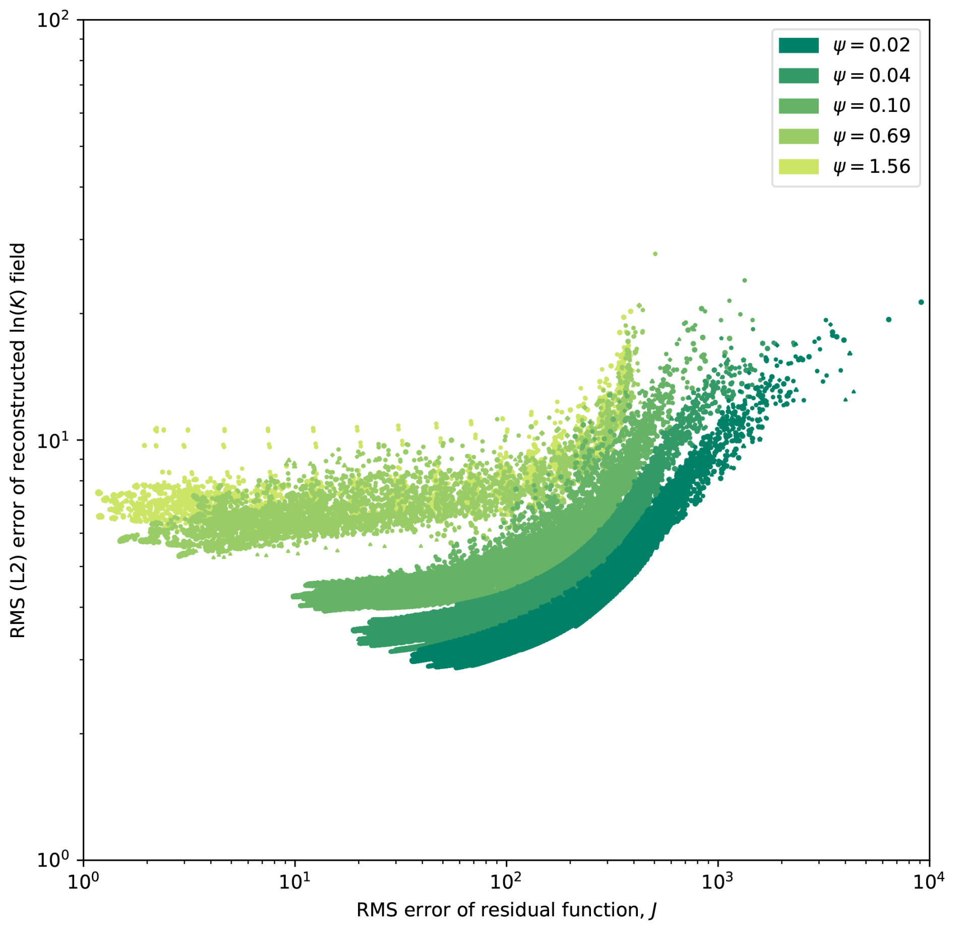
Figure 2 Comparison of the L² error of the reconstructed hydraulic conductivity field versus the residual function, J, defined in Eq. (3) for several different measurement densities, Ψ, in the main MC study. Weights are as defined in Eqs. (37)–(40). Each ensemble is plotted with a unique color, and within each ensemble, each parameter iteration for each calibration trial (i.e., unique pairing of ζ and p⁰) is shown.

4.2 Feature scale and information gain due to calibration

A second illuminating analysis that can be performed on the main MC study is to consider the average improvement of each individual K–L coefficient, indexed by T, the basis function wavelength normalized to the measurement spacing. This allows us to determine the ability to identify features of a particular scale by calibration and to determine a cutoff beneath which small-scale variability is essentially invisible to the calibration process. In Fig. 3, the average ratio of squared coefficient error after vs. before calibration is shown as a function of T for each calibrated K–L basis function, for all five ensembles, each for a different value of Ψ. For small T, we observe a relatively flat (relative to T) regime in which only minor improvement is observed. We attribute the improvement to the w_R regularization term, for reasons discussed below. Around T = 4, we observe a sharp regime change, in which r begins to rapidly decrease in a power-law fashion with increasing T; we identify the following empirical relation for this regime:

48

shown as the dotted line in Fig. 3. A consequence of this analysis is that positive identification becomes possible only once feature scale exceeds 4 times the measurement spacing. We note good coherence between the various ensembles, suggesting that T is an adequate metric for capturing relative basis function scale.

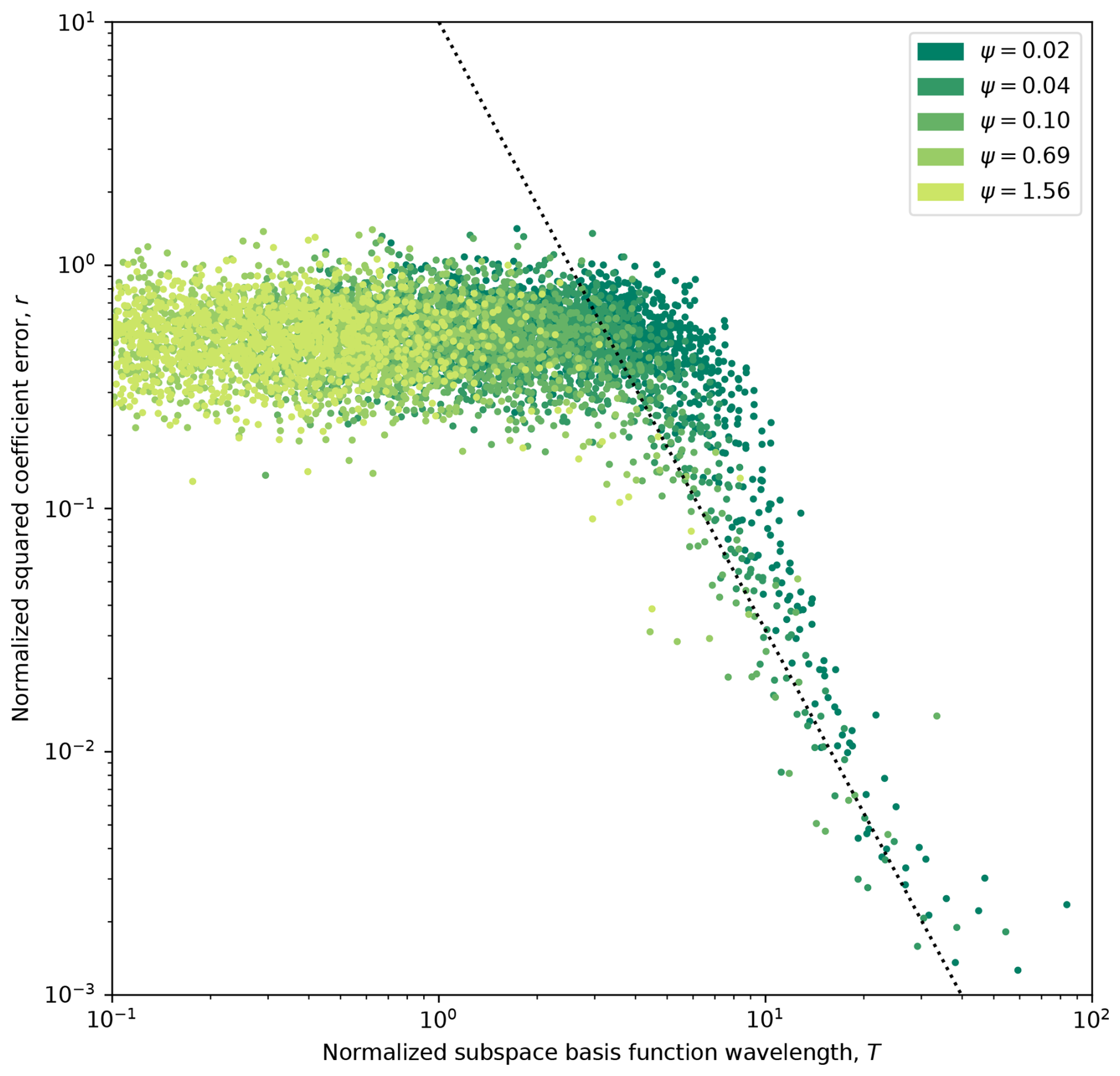
Figure 3 Geometric mean-squared relative coefficient error improvement, r, for each K–L basis function, f_n(x), across all calibration trials (i.e., unique pairing of ζ and p⁰) in each ensemble (corresponding to a different value of Ψ) in the main MC study. Each basis function is represented by its normalized wavelength, T, rather than its index. A dashed trend line scaling as T^−2.5 is shown in the long-wavelength region.

4.3 Information gain due to velocity measurements and regularization

In the second MC study, we fixed Ψ = 0.10 but modified the objective function in various ways to ascertain how the modifications affect the L² accuracy of the ultimate reconstruction ($L_{\mathrm{2000}}^{\mathrm{2}}$) and also the ability to calibrate large-scale features in the 12-dimensional subspace spanned by the K–L basis functions satisfying the previously identified criterion T > 4 ($L_{\mathrm{12}}^{\mathrm{2}}$). The specifics of the studies and the resulting metrics are tabulated in Table 1. A visual representation of the amount of learning that occurs about the coefficients of each K–L basis function, sorted by T, analogous to the one for the main study is shown in Fig. 4.

Table 1 Descriptive statistics of five ensemble calibration experiments in the second MC study, corresponding to Ψ = 0.1.

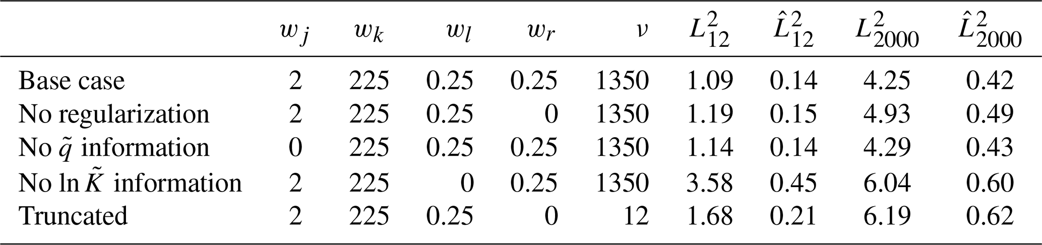
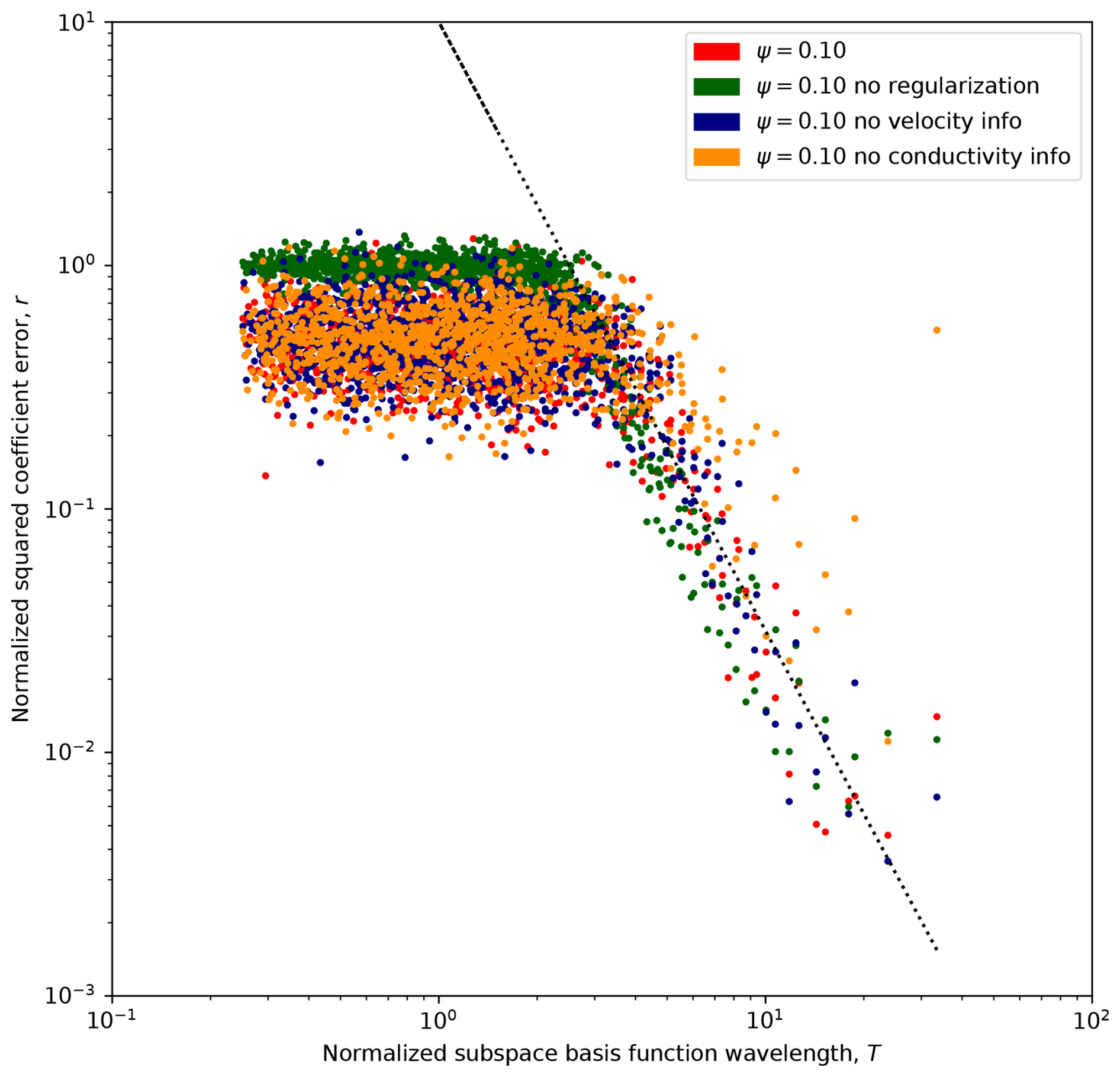
Figure 4 Geometric mean-squared relative coefficient error improvement, r, across all calibration trials in each ensemble in the second MC study. Results are presented as a function of normalized K–L basis function wavelength, T, with each ensemble representing different terms present in the loss function. A dashed trend line scaling as T^−2.5 is shown in the long-wavelength region.

In this study, the base case (featuring all available information) was shared with the main MC study. In this data set, calibration was performed beginning from a pair of different random p⁰ vectors for each true field vector, ζ. Visual examination of the calibrated head fields for this data set showed that the fitted ln K and h fields were in all cases visually identical for both of the paired initial parameter guesses. This suggests that the regularized objective function was convex, and that the unique solution is essentially found in all cases, with no influence of initial conditions. However, even when the unique regularized solution is achieved, the remaining relative error, ${\widehat{L}}_{\mathrm{2000}}^{\mathrm{2}}$, is still 42 %, and it is 12 % in the subspace spanned by the most significant (longest wavelength) basis functions. Figure 1a visually illustrates the results; note how large-scale features are captured, but there is still significant infidelity between the smooth, regularized ln K and the true $\ln \stackrel{\mathrm{̃}}{K}$. By calibration, L² error is reduced to 32 % of its value in the initial guess.

Where regularization is disabled, pairwise visual comparison reveals some residual effect of initial guess vector, although large-scale features of the true fields are plainly always captured. The unregularized calibrated L² error was only slightly worse than for regularized calibration in the most significant subspace (again see Table 1), attributable to the fact that the data are highly informative on these K–L coefficients, and there is limited work for regularization to accomplish. For the unregularized ensemble, we attribute residual L² error to errors in high-wavenumber subspaces from the initial guess p⁰ that manifest at locations remote from the measurements and which are left over after large-scale features have been identified. This is an entirely different cause of errors than the smoothing which generates unique solutions in the w_R-regularized case. Figure 1b illustrates unregularized calibration using the same target field and measurement data as used in panel (a). By calibration, L² error is reduced to 34 % of its value in the initial guess, and the final absolute L² error for panel (b) is 24 % higher than for panel (a).

Without regularization from w_R, r≈ 1 in the T < 4 subspace corresponding to small-scale features, indicating that the measurements provide no information about these coefficients. We attribute the improved performance with the regularization term to the fact that the coefficients of ζ and p⁰ are all independent identically distributed random variables ∼ 𝒩(0,1); it is easy to show that $\text{Var}({\mathit{\zeta }}_n-p_n^{\mathrm{0}})>\text{Var}\left({\mathit{\zeta }}_n\right)$ = 1, so by pulling each p_n towards zero, the w_R term in J decreases average square error of p_n, even without any information from the measurements regarding its value.

A previous study (Tso et al., 2016), performed using a different co-kriging-based calibration approach, suggested a significant gain in reconstruction reliability over use of head–conductivity co-kriging. We tested whether groundwater speed would provide similar extra information in the context of gradient-descent model calibration by performing a calibration ensemble in which its weight was zero. We found performance essentially identical to that for the base case. Given that head and conductivity fields jointly determine the flux everywhere, and regularization is sufficient to determine a unique solution, the fact that speed information was found to be redundant implies that the regularized solution correctly identifies $\stackrel{\mathrm{̃}}{h}$ and $\stackrel{\mathrm{̃}}{K}$ at the measurement locations.

Given the idea that a correct speed and head field could uniquely determine $\stackrel{\mathrm{̃}}{K}$ everywhere, we examined the extent to which speed measurements could substitute for hard-to-determine point measurements of $\stackrel{\mathrm{̃}}{K}$ by eliminating the weight on these measurements in J. This was found to be possible to some extent, but performance was significantly reduced relative to all other approaches, with identification in the most significant long-wavelength subspaces, as measured by $L_{\mathrm{12}}^{\mathrm{2}}$, significantly degraded. A possible explanation for this result is that calibration of $\stackrel{\mathrm{̃}}{K}$ becomes sensitive to errors in ∇h as well as h.

Finally, motivated by the idea that the long-wavelength subspace (T > 4) is readily identifiable without regularization, and that the measurements contain little or no information about the small-T (small-scale feature) subspace, we attempted a naive truncation-based regularization approach in which only the most significant T > 4 K–L coefficients are calibrated (the rest are fixed to 0), and no regularization term is applied (i.e., ν = 12 and w_R = 0 for this ensemble). Performance of this approach was not as strong as the other trials, with ${\widehat{L}}_{\mathrm{12}}^{\mathrm{2}}$ = 0.21, about 50 % greater than in the base case, but identification of the large-scale subspace remained respectable and still exceeded the regularized trial with no $\ln \stackrel{\mathrm{̃}}{K}$ measurements. When the K–L field representation is employed, $\partial K/\partial p_n$ does not collapse to unity, so there remains an expensive basis-function-specific integration in Eq. (9). Thus, the computational cost of computing the gradient using naive truncation was reduced more than 100-fold in this ensemble relative to the base case, and this approach merits further consideration.

4.4 Can we expect these results to generalize?

Both the identification cutoff of 4 times the measurement scale and the observation of the power-law improvement of identifiability with increased feature scale are empirical results of an MC study. As with any empirical investigation, it is natural to wonder how general the results are, or whether they are dependent in some way on the specific setting chosen for the study. In our investigations, these relations were found to be robust to changed point measurement resolution and also to zero weighting of certain types of measurements and different regularization schemes, suggesting robustness to alteration of the objective function.

Regarding the specifics of correlation structure and average gradient, it is helpful to recall that the point measurements functionally constrain a low-order 2D Taylor series expansion of the head near each measurement location, and that an accurate head field can be uniquely inverted to recover the underlying conductivity field. It is thus reasonable to attribute the weaker identification of smaller-scale features to their proportionally larger impact on higher-order terms of the head field, which do not impact the observed quantities. The decreased visibility of smaller-scale features due to non-unique impact on observables on this analysis is a direct result of feature scale normalized to the measurement scale (i.e., T). Consequently, we do not expect the details of correlation structure or large-scale flow regime to impact our results.

By contrast, it is well documented that behavior of physical processes such as Darcy flow may be affected by system dimension (e.g., Chiogna et al., 2014). So while we follow the example of much previous research in focusing on reconstruction of 2D conductivity (equivalently, transmissivity) fields, a valuable follow-up would consider identifiability of full 3D conductivity fields.

5 Summary and conclusions

We computed the sensitivity of a loss function based on three types of point hydraulic measurements and a general regularization term to an underlying, heterogeneous hydraulic conductivity field via a continuous adjoint-state approach. Using K–L expansion, we created a general, zonation-free technique for analyzing the quality of inversion from point data to an underlying heterogeneous scalar field. Using K–L basis functions which feature clearly defined wavelengths, we analyzed how reliably conductivity and head fields were recovered, both as a function of feature scale and globally, given different densities and types of point measurements.

The following are our key conclusions:

• Substantially better than random identification accuracy was observed once K field feature scales exceed 4 times the measurement spacing, with relative squared error after calibration scaling as T^−2.5, where T is feature scale normalized to measurement spacing. This relation provides a useful guideline for needed measurement density to achieve desired field reconstruction accuracy. For higher-resolution characterization, non-point geophysical or tracer data may be required.

• Even at very coarse measurement resolutions relative to K field correlation length, the pointwise loss function was found informative globally (in an L² sense) about the underlying conductivity field, and calibration offers better than random feature identification at all scales when regularization is employed.

• Groundwater speed point measurements were found to partially substitute for point conductivity measurements but, contrary to the sequential linear estimation study of Tso et al. (2016), provide little additional information in the context of regularized gradient-descent optimization of point prediction errors, provided reliable head and conductivity point measurements already exist.

• The gradient-descent calibration ultimate L² error was found to be dependent on measurement density and displays quickly diminishing returns on optimization. We posit that large-scale features are identified quickly, and that the loss function is less sensitive to point mismatch remote from the measurement locations. Thus, later iterations tend to optimize field values near the well: K-field infidelity remote from the measurement locations that exists by the time large-scale features have been identified tends to persist.

The approach adopted here has a number of useful features that may be helpful for further investigations. The analytical sensitivity expression for a loss function containing many different types of data and regularization can be used for model fitting, and its zonated form, Eq. (8), is particularly efficient for use with finite-volume and finite-element codes. Also, this sort of zonation-free K–L series Monte Carlo calibration study could be used to explore the identifiability of other geophysical fields, beyond the hydraulic conductivity/transmissivity fields considered in this study. Naturally, as the relations uncovered herein are empirically based, it is possible they may depend in some way on the specific model chosen for the study. Exploration in 3D may in particular be profitable.

Appendix A: Adjoint sensitivity equation derivation

The sensitivity of J, Eq. (3), to any given model parameter, p_i, can be computed directly:

$$\begin{array}{}\text{(A1)}& \begin{array}{rl}& {\displaystyle \frac{\partial J}{\partial p_i}}\\ & =\sum _j\mathrm{2}{w}_j\left(K\left({\mathit{x}}_j\right)∥\mathrm{\nabla }h\left({\mathit{x}}_j\right)∥-\stackrel{\mathrm{̃}}{q}\left({\mathit{x}}_j\right)\right)\\ & \left[{\displaystyle \frac{\partial K}{\partial p_i}}∥\mathrm{\nabla }h\left({\mathit{x}}_j\right)∥+K{\displaystyle \frac{\mathrm{\nabla }h\cdot \mathrm{\nabla }{\mathit{\varphi }}_i}{∥\mathrm{\nabla }h∥}}\right]\\ & +\sum _k\mathrm{2}{w}_k{\mathit{\varphi }}_i\left({\mathit{x}}_k\right)\left(h\left({\mathit{x}}_k\right)-\stackrel{\mathrm{̃}}{h}\left({\mathit{x}}_k\right)\right)\\ & +\sum _l\mathrm{2}{w}_l{\displaystyle \frac{\mathrm{1}}{K\left({\mathit{x}}_l\right)}}{\displaystyle \frac{\partial K}{\partial p_i}}\left(\ln K\left({\mathit{x}}_l\right)-\ln \stackrel{\mathrm{̃}}{K}\left({\mathit{x}}_l\right)\right)+{\displaystyle \frac{\partial R}{\partial p_i}},\end{array}\end{array}$$

where we define the sensitivity ${\mathit{\varphi }}_i\equiv \partial h/\partial p_i$. Employing the vector form and rewriting in terms of integrals over the volume Ω:

$$\begin{array}{}\text{(A2)}& \begin{array}{rl}{\displaystyle \frac{\partial J}{\partial \mathit{p}}}=& \underset{\mathrm{\Omega }}{\int }\mathrm{2}\left(K∥\mathrm{\nabla }h∥-\stackrel{\mathrm{̃}}{q}\right){\displaystyle \frac{\partial K}{\partial \mathit{p}}}∥\mathrm{\nabla }h∥\sum _j{w}_j\mathit{\delta }(\mathit{x}-{\mathit{x}}_j)\mathrm{d}V\\ & +\underset{\mathrm{\Omega }}{\int }\mathrm{2}\left(K∥\mathrm{\nabla }h∥-\stackrel{\mathrm{̃}}{q}\right)K{\displaystyle \frac{\mathrm{\nabla }h\cdot \mathrm{\nabla }\mathit{\varphi }}{∥\mathrm{\nabla }h∥}}\sum _j{w}_j\mathit{\delta }(\mathit{x}-{\mathit{x}}_j)\mathrm{d}V\\ & +\underset{\mathrm{\Omega }}{\int }\mathrm{2}\mathit{\varphi }\left(h-\stackrel{\mathrm{̃}}{h}\right)\sum _k{w}_k\mathit{\delta }(\mathit{x}-{\mathit{x}}_k)\mathrm{d}V\\ & +\underset{\mathrm{\Omega }}{\int }\mathrm{2}{\displaystyle \frac{\mathrm{1}}{K}}{\displaystyle \frac{\partial K}{\partial \mathit{p}}}\left(\ln K-\ln \stackrel{\mathrm{̃}}{K}\right)\sum _l{w}_l\mathit{\delta }(\mathit{x}-{\mathit{x}}_l)\mathrm{d}V\\ & +{\displaystyle \frac{\partial R}{\partial \mathit{p}}}.\end{array}\end{array}$$

Simplifying the second integral by employing integration by parts to remove the dependence on ∇ϕ and then employing Eq. (1) yields

$$\begin{array}{}\text{(A3)}& \begin{array}{rl}{\displaystyle \frac{\partial J}{\partial \mathit{p}}}=& \underset{\mathrm{\Omega }}{\int }\mathrm{2}\left(K∥\mathrm{\nabla }h∥-\stackrel{\mathrm{̃}}{q}\right){\displaystyle \frac{\partial K}{\partial \mathit{p}}}∥\mathrm{\nabla }h∥\sum _j{w}_j\mathit{\delta }(\mathit{x}-{\mathit{x}}_j)\mathrm{d}V\\ & -\underset{\mathrm{\Omega }}{\int }\mathrm{2}\mathit{\varphi }K\mathrm{\nabla }h\cdot \mathrm{\nabla }\left[\left(K-{\displaystyle \frac{\stackrel{\mathrm{̃}}{q}}{∥\mathrm{\nabla }h∥}}\right)\sum _j{w}_j\mathit{\delta }(\mathit{x}-{\mathit{x}}_j)\right]\mathrm{d}V\\ & +\underset{\mathrm{\Omega }}{\int }\mathrm{2}\mathit{\varphi }\left(h-\stackrel{\mathrm{̃}}{h}\right)\sum _k{w}_k\mathit{\delta }(\mathit{x}-{\mathit{x}}_k)\mathrm{d}V\\ & +\underset{\mathrm{\Omega }}{\int }\mathrm{2}{\displaystyle \frac{\mathrm{1}}{K}}{\displaystyle \frac{\partial K}{\partial \mathit{p}}}\left(\ln K-\ln \stackrel{\mathrm{̃}}{K}\right)\sum _l{w}_l\mathit{\delta }(\mathit{x}-{\mathit{x}}_l)\mathrm{d}V\\ & +{\displaystyle \frac{\partial R}{\partial \mathit{p}}}.\end{array}\end{array}$$

A1 Weak-form equation for sensitivity

We may differentiate Eqs. (1)–(2) with respect to p so as to generate a BVP for the sensitivity vector, ϕ:

$$\begin{array}{}\text{(A4)}& {\displaystyle }\mathrm{\nabla }\cdot \left({\displaystyle \frac{\partial K}{\partial \mathit{p}}}\mathrm{\nabla }h\right)+\mathrm{\nabla }\cdot \left(K\mathrm{\nabla }\mathit{\varphi }\right)=\mathrm{0}\text{in}\mathrm{\Omega },\text{(A5)}& {\displaystyle }\mathit{\varphi }={\displaystyle \frac{\partial f}{\partial \mathit{p}}}\text{on}\mathit{\delta }\mathrm{\Omega }.\end{array}$$

The sensitivity equation, Eq. (A4), can be placed in the weak form by expressing it as an integral with respect to ϕ^*, an arbitrary smooth test function known as the adjoint:

$$\begin{array}{}\text{(A6)}& \underset{\mathrm{\Omega }}{\int }\left[\mathrm{\nabla }\cdot \left({\displaystyle \frac{\partial K}{\partial \mathit{p}}}\mathrm{\nabla }h\right)\right]{\mathit{\varphi }}^{*}\mathrm{d}V+\underset{\mathrm{\Omega }}{\int }\left[\mathrm{\nabla }\cdot \left(K\mathrm{\nabla }\mathit{\varphi }\right)\right]{\mathit{\varphi }}^{*}\mathrm{d}V=\mathrm{0}.\end{array}$$

We then integrate the first integral by parts once and the second by parts twice to arrive at the five-term expression

$$\begin{array}{}\text{(A7)}& \begin{array}{rl}\mathrm{0}=& \underset{\mathit{\delta }\mathrm{\Omega }}{\int }{\displaystyle \frac{\partial K}{\partial \mathit{p}}}\mathrm{\nabla }h{\mathit{\varphi }}^{*}\cdot \mathrm{d}S-\underset{\mathrm{\Omega }}{\int }{\displaystyle \frac{\partial K}{\partial \mathit{p}}}\mathrm{\nabla }h\cdot \mathrm{\nabla }{\mathit{\varphi }}^{*}\mathrm{d}V\\ & +\underset{\mathit{\delta }\mathrm{\Omega }}{\int }K\mathrm{\nabla }\mathit{\varphi }{\mathit{\varphi }}^{*}\cdot \mathrm{d}S-\underset{\mathit{\delta }\mathrm{\Omega }}{\int }K\mathit{\varphi }\mathrm{\nabla }{\mathit{\varphi }}^{*}\cdot \mathrm{d}S\\ & +\underset{\mathrm{\Omega }}{\int }\mathit{\varphi }\mathrm{\nabla }\cdot \left(K\mathrm{\nabla }{\mathit{\varphi }}^{*}\right)\mathrm{d}V.\end{array}\end{array}$$

A2 Removing derivatives of ϕ and simplifying

Our goal is to derive an equation for $\frac{\partial J}{\partial \mathit{p}}$ that does not explicitly depend on ϕ. To this end, we add Eqs. (A3) and (A7) to generate

$$\begin{array}{}\text{(A8)}& \begin{array}{rl}& {\displaystyle \frac{\partial J}{\partial \mathit{p}}}\\ & =\underset{\mathrm{\Omega }}{\int }\mathrm{2}\left(K∥\mathrm{\nabla }h∥-\stackrel{\mathrm{̃}}{q}\right){\displaystyle \frac{\partial K}{\partial \mathit{p}}}∥\mathrm{\nabla }h∥\sum _j{w}_j\mathit{\delta }(\mathit{x}-{\mathit{x}}_j)\mathrm{d}V\\ & -\underset{\mathrm{\Omega }}{\int }\mathrm{2}\mathit{\varphi }K\mathrm{\nabla }h\cdot \mathrm{\nabla }\left[\left(K-{\displaystyle \frac{\stackrel{\mathrm{̃}}{q}}{∥\mathrm{\nabla }h∥}}\right)\sum _j{w}_j\mathit{\delta }(\mathit{x}-{\mathit{x}}_j)\right]\mathrm{d}V\\ & +\underset{\mathrm{\Omega }}{\int }\mathrm{2}\mathit{\varphi }\left(h-\stackrel{\mathrm{̃}}{h}\right)\sum _k{w}_k\mathit{\delta }(\mathit{x}-{\mathit{x}}_k)\mathrm{d}V\\ & +\underset{\mathrm{\Omega }}{\int }{\displaystyle \frac{\mathrm{2}}{K}}{\displaystyle \frac{\partial K}{\partial \mathit{p}}}\left(\ln K-\ln \stackrel{\mathrm{̃}}{K}\right)\sum _l{w}_l\mathit{\delta }(\mathit{x}-{\mathit{x}}_l)\mathrm{d}V+{\displaystyle \frac{\partial R}{\partial \mathit{p}}}\\ & +\underset{\mathit{\delta }\mathrm{\Omega }}{\int }{\displaystyle \frac{\partial K}{\partial \mathit{p}}}\mathrm{\nabla }h{\mathit{\varphi }}^{*}\cdot \mathrm{d}S-\underset{\mathrm{\Omega }}{\int }{\displaystyle \frac{\partial K}{\partial \mathit{p}}}\mathrm{\nabla }h\cdot \mathrm{\nabla }{\mathit{\varphi }}^{*}\mathrm{d}V\\ & +\underset{\mathit{\delta }\mathrm{\Omega }}{\int }K\mathrm{\nabla }\mathit{\varphi }{\mathit{\varphi }}^{*}\cdot \mathrm{d}S-\underset{\mathit{\delta }\mathrm{\Omega }}{\int }K\mathit{\varphi }\mathrm{\nabla }{\mathit{\varphi }}^{*}\cdot \mathrm{d}S\\ & +\underset{\mathrm{\Omega }}{\int }\mathit{\varphi }\mathrm{\nabla }\cdot \left(K\mathrm{\nabla }{\mathit{\varphi }}^{*}\right)\mathrm{d}V.\end{array}\end{array}$$

We ultimately want to remove the dependence on ϕ, so we combine the volume integrals whose integrands are proportional to it:

$$\begin{array}{}\text{(A9)}& \begin{array}{rl}& {\displaystyle \frac{\partial J}{\partial \mathit{p}}}\\ & =\underset{\mathrm{\Omega }}{\int }\mathit{\varphi }[\mathrm{\nabla }\cdot (K\mathrm{\nabla }{\mathit{\varphi }}^{*})-\mathrm{2}K\mathrm{\nabla }h\\ & \cdot \mathrm{\nabla }\left(\left(K-{\displaystyle \frac{\stackrel{\mathrm{̃}}{q}}{∥\mathrm{\nabla }h∥}}\right)\sum _j{w}_j\mathit{\delta }(\mathit{x}-{\mathit{x}}_j)\right)\\ & +\mathrm{2}\left(h-\stackrel{\mathrm{̃}}{h}\right)\sum _k{w}_k\mathit{\delta }(\mathit{x}-{\mathit{x}}_k)]\mathrm{d}V\\ & +\underset{\mathrm{\Omega }}{\int }\mathrm{2}\left(K∥\mathrm{\nabla }h∥-\stackrel{\mathrm{̃}}{q}\right){\displaystyle \frac{\partial K}{\partial \mathit{p}}}∥\mathrm{\nabla }h∥\sum _j{w}_j\mathit{\delta }(\mathit{x}-{\mathit{x}}_j)\mathrm{d}V\\ & +\underset{\mathrm{\Omega }}{\int }{\displaystyle \frac{\mathrm{2}}{K}}{\displaystyle \frac{\partial K}{\partial \mathit{p}}}\left(\ln K-\ln \stackrel{\mathrm{̃}}{K}\right)\sum _l{w}_l\mathit{\delta }(\mathit{x}-{\mathit{x}}_l)\mathrm{d}V+{\displaystyle \frac{\partial R}{\partial \mathit{p}}}\\ & -\underset{\mathrm{\Omega }}{\int }{\displaystyle \frac{\partial K}{\partial \mathit{p}}}\mathrm{\nabla }h\cdot \mathrm{\nabla }{\mathit{\varphi }}^{*}\mathrm{d}V+\underset{\mathit{\delta }\mathrm{\Omega }}{\int }{\displaystyle \frac{\partial K}{\partial \mathit{p}}}\mathrm{\nabla }h{\mathit{\varphi }}^{*}\cdot \mathrm{d}S\\ & +\underset{\mathit{\delta }\mathrm{\Omega }}{\int }K\mathrm{\nabla }\mathit{\varphi }{\mathit{\varphi }}^{*}\cdot \mathrm{d}S-\underset{\mathit{\delta }\mathrm{\Omega }}{\int }K\mathit{\varphi }\mathrm{\nabla }{\mathit{\varphi }}^{*}\cdot \mathrm{d}S.\end{array}\end{array}$$

The first integral (and its dependence on the ϕ) is removed if the expression in the square brackets is zero, implying that

$$\begin{array}{}\text{(A10)}& \begin{array}{rl}& \underset{\mathrm{\Omega }}{\int }\mathrm{\nabla }\cdot \left(K\mathrm{\nabla }{\mathit{\varphi }}^{*}\right)\\ & -\mathrm{2}K\mathrm{\nabla }h\cdot \mathrm{\nabla }\left(\left(K-{\displaystyle \frac{\stackrel{\mathrm{̃}}{q}}{∥\mathrm{\nabla }h∥}}\right)\sum _j{w}_j\mathit{\delta }(\mathit{x}-{\mathit{x}}_j)\right)\\ & +\mathrm{2}\left(h-\stackrel{\mathrm{̃}}{h}\right)\sum _k{w}_k\mathit{\delta }(\mathit{x}-{\mathit{x}}_k)\mathrm{d}V=\mathrm{0}.\end{array}\end{array}$$

Applying integration by parts to the second term of the integrand and then applying Eq. (1) allows for the simplification:

$$\begin{array}{}\text{(A11)}& \underset{\mathrm{\Omega }}{\int }\mathrm{\nabla }\cdot \left(K\mathrm{\nabla }{\mathit{\varphi }}^{*}\right)+\mathrm{2}\left(h-\stackrel{\mathrm{̃}}{h}\right)\sum _k{w}_k\mathit{\delta }(\mathit{x}-{\mathit{x}}_k)\mathrm{d}V=\mathrm{0}\end{array}$$

This motivates solution of an adjoint problem in ϕ^* to eliminate the dependence of Eq. (A9) on ϕ. See Sect. 2.2 for the result.