Effects of boundary conditions and aquifer parameters on salinity distribution and mixing-controlled reactions in high-energy beach aquifers

In high-energy beach aquifers fresh groundwater mixes with recirculating saltwater and biogeochemical reactions modify the composition of groundwater discharging to the sea. Changing beach morphology, hydrodynamic forces, and hydrogeological properties control density-driven groundwater flow and transport processes that affect the distribution of chemical reactants. In the present study, density-driven flow and transport modelling of a generic 2-D cross-shore transect was conducted. Boundary conditions and aquifer parameters were varied in a systematic manner in a suite of 24 cases. The objective was to investigate the individual effects of boundary conditions and hydrogeological parameters on flow regime, salt distribution, and potential for mixing-controlled chemical reactions in a system with a temporally variable beach morphology. Our results show that a changing beach morphology causes the migration of infiltration and exfiltration locations along the beach transect, leading to transient flow and salt transport patterns in the subsurface, thereby enhancing mixing-controlled reactions. The shape and extent of the zone where mixing-controlled reactions potentially take place, as well as the spatiotemporal variability of the freshwater–saltwater interfaces, are most sensitive to variable beach morphology, storm floods, hydraulic conductivity, and dispersivity. The present study advances the understanding of subsurface flow, transport, and mixing processes that are dynamic beneath high-energy beaches. These processes control biogeochemical reactions that regulate nutrient fluxes to coastal ecosystems.

1 Introduction

Sandy beaches make up about 30 % of the world's coastline (Luijendijk et al., 2018) and form the transition zone between the terrestrial and marine environment. The subsurface part of this transition zone is called a subterranean estuary (STE) (Moore, 1999; Robinson et al., 2006). Here, two water bodies, terrestrial fresh groundwater and recirculating sea water, distinct in physical properties and chemical composition (e.g. density, temperature, pH, redox state), mix and (bio)geochemical reactions take place that change the composition of the water (Anschutz et al., 2009). These reactions and resulting element fluxes across the land–sea interface are linked to residence times and dispersive mixing processes that depend on dynamic density-driven groundwater flow and transport processes (Anwar et al., 2014; Robinson et al., 2009; Spiteri et al., 2008).

The established concept of flow and transport patterns in the STE describes the relatively stable formation of three water bodies: the freshwater discharge tube (FDT) separates the wave- and tide-induced upper saline plume (USP) from the saltwater wedge (SW) (Robinson et al., 2006, 2018). At the interfaces of the water bodies, dispersive mixing zones develop. The extent of the mixing zone where (bio)geochemical reactions take place depends on the geological conditions and (hydro)dynamic forces (Michael et al., 2016; Robinson et al., 2018). In a homogenous aquifer, three distinct Darcy velocity regimes exist: (1) very low velocities in the SW, (2) high velocities in the discharge zone of the FDT, and (3) uniform velocities in the coastal aquifer on the landward side (Costall et al., 2020). The geological architecture and resulting hydrogeological parameters define the connection of the land–sea interface and affect the development and extension of the mixing zone where (bio)geochemical reactions take place. Not only larger geological structures, like paleo-channels (Meyer et al., 2018b, 2019; Mulligan et al., 2007), but also fine-scale aquifer heterogeneity coupled with tides (Geng et al., 2020) create more complex flow paths for both intruding seawater (SWI) and discharging groundwater rich in nutrients. Costall et al. (2020) demonstrated the effect of heterogeneous hydraulic conductivity on the nearshore flow regime, resulting in highly variable flow directions and velocities. Michael et al. (2016) showed that geologic complexity in terms of heterogeneous hydraulic conductivity and anisotropy enhances mixing and focuses the flow across the land–sea interface. Abarca et al. (2007) investigated the effect of longitudinal α_L and transverse α_T dispersivity on the thickness of the mixing zone and found that both contribute to the same extent but each in a different part of the mixing zone.

The impact of hydrodynamic forces such as tides, waves, and storm surges on flow regimes and the salinity pattern in the STE environment has been comprehensively studied (e.g. Michael et al., 2016; Robinson et al., 2018). However, most of these studies focused on low-energy environments like lagoons (Müller et al., 2021) or bays, while high-energy beaches, with high tidal amplitudes and/or high waves, were studied less, although they are particularly affected by tides, waves, and storms (Massmann et al., 2023). Hydraulic and atmospheric forces also continuously re-shape the beach morphology by erosion and accretion processes (Short and Jackson, 2013) that in turn change the hydraulic gradients in the beach subsurface and hence affect the flow and transport regime. It has been recognized that the beach topography has an impact on the subsurface salinity distribution (Abarca et al., 2013; Grünenbaum et al., 2020b; Robinson et al., 2006). Studies have provided field evidence supported by numerical models for the – at least temporal – occurrence of more than one USP for different beach slopes (Abarca et al., 2013) or typical sandy beach surfaces like runnel-ridge (Grünenbaum et al., 2020b) and through-berm (Robinson et al., 2006) structures. Robinson et al. (2006) concluded that the beach morphology combined with a tidal signal significantly affects the flow and recirculation of seawater in the STE and hypothesized that combined with waves this would enhance the exchange of water across the land–sea interface and would lead to more complex flow patterns. However, none of the aforementioned studies implemented a transient, continuously changing beach morphology in their groundwater models. Using a density-dependent groundwater flow and transport model, Greskowiak and Massmann (2021) demonstrated that a transient beach morphology combined with seasonal storm floods led to strong spatiotemporal variability in groundwater flow and transport patterns. In their model, the effects of the morphodynamics reached tens of metres into the subsurface and distorted the typical salinity stratification in the STE. In a next step, Greskowiak et al. (2023) extended the approach by a numerical reactive transport model, analysed the development of redox zones, and concluded that redox zone dynamics in the STE are strongly affected by beach morphodynamics. While some redox reactions take place in the USPs and storm-flood-affected area, mixing-controlled reactions driven by mixing of two solutes in different end members occur in the fringes of the USP and at the SW interface (Heiss et al., 2017). Real-world examples relevant in STE environments for these mixing-controlled reactions are iron curtain formation (Charette and Sholkovitz, 2002) and nitrification (Ullman et al., 2003). Anwar et al. (2014) studied the impact of tides and waves on mixing-dependent reactions and concluded that they intensify seawater–freshwater mixing and nutrient transformations, resulting in enhanced fluxes to the sea. In addition, Heiss et al. (2017) found that tidal amplitude and hydraulic conductivity are the factors that have the strongest effect on nitrate transformation and that the size of the mixing zone as well as solute supply defines the mixing-dependent reactivity.

In their review on geochemical fluxes in sandy beaches Geng et al. (2021) disclosed the need for coupling shoreline morphology and groundwater flow. As Greskowiak and Massmann (2021) showed this is particularly relevant in the understudied environment of high-energy beaches, since these are exposed to strong hydrodynamic and atmospheric forces (Massmann et al., 2023) and hence experience profound changes in beach morphology (Montaño et al., 2020). This in turn shows significant effects on the flow and transport regime reaching deep into the subsurface and impacts the mixing-controlled reactions and hence the exchange and transformation of nutrients across the land–sea transition zone.

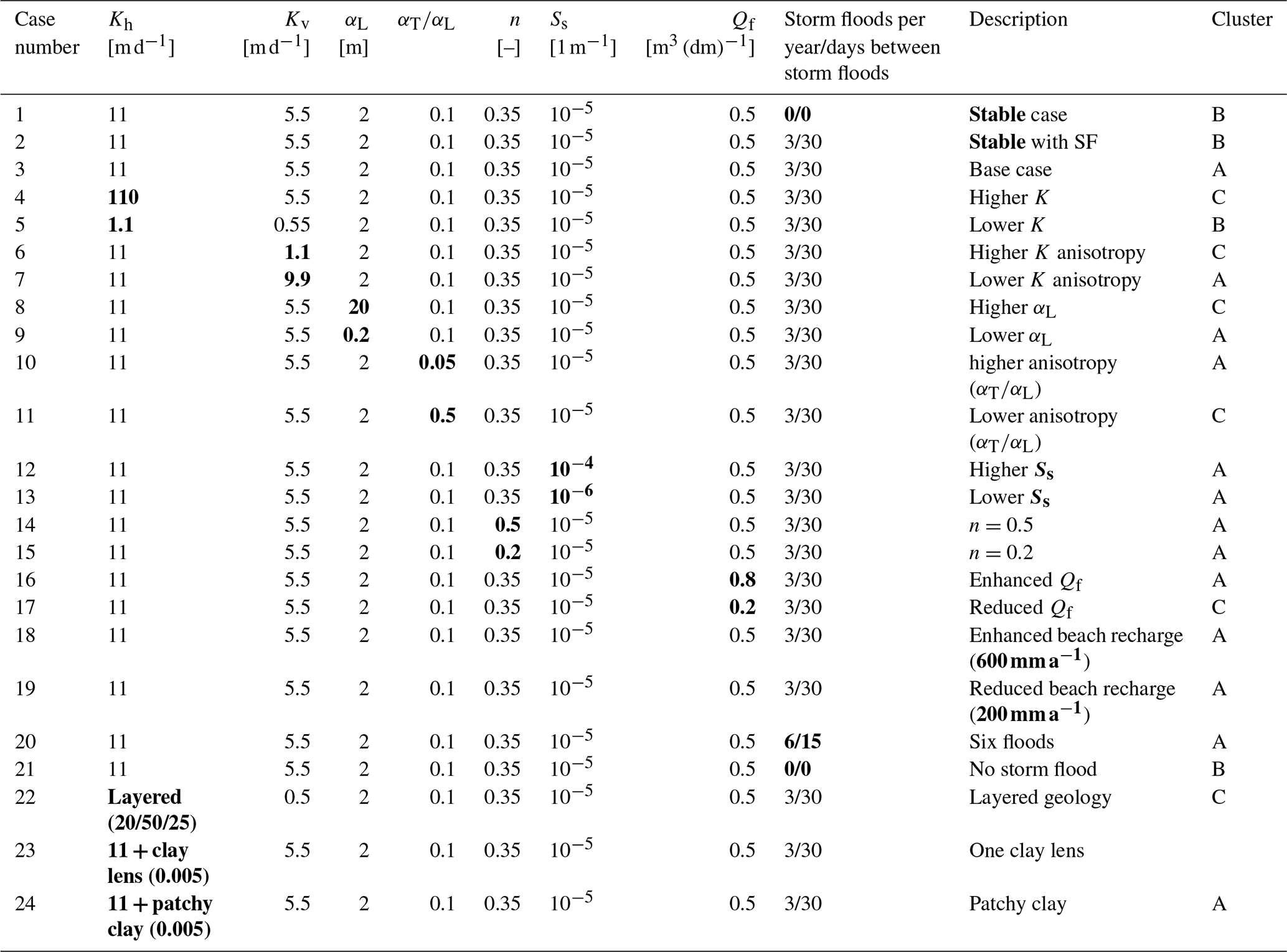
Table 1 Aquifer properties and boundary conditions for the 24 model cases. Numbers in bold highlight the changes compared to the base case. Note that the base case is a case with dynamic topography resembling the model by Greskowiak and Massmann (2021) and a beach recharge of 400 mm a⁻¹.

The objective of the present study is to investigate the interplay of morphological changes and hydrodynamic boundary conditions paired with aquifer properties in the subsurface of high-energy beaches in a 2-D density-dependent generic modelling approach. Our model is considered “generic” because it does not aim to replicate specific site conditions using field data or calibration. Instead, boundary conditions and parameters are varied to explore physical processes in STEs. While based on Spiekeroog's conditions, the model aims to represent barrier islands in high-energy environments like the Wadden Sea, rather than a specific location. The aims of the study are to systematically evaluate the effect of hydrogeological parameters, i.e. horizontal (K_h) and vertical (K_v) hydraulic conductivities, longitudinal (α_L) and transversal (α_T) dispersivities, porosity (n) and specific storage (S_s), and boundary conditions (freshwater inflow, recharge, storm surges) combined with varying beach morphology on (1) the flow regime, (2) the distribution of total dissolved solids (TDSs) and their temporal concentration variability calculated as the standard deviation of TDSs, and (3) the potential extent to which mixing-controlled chemical reactions occur, hereafter called “mixing-controlled reaction potential”. By closing this research gap, the present study advances the understanding of subsurface processes in STEs underneath high-energy beaches that alter the composition of water discharging into the sea.

2 Material and methods

We used a 2-D generic modelling approach loosely based on real field conditions of the east Frisian barrier island Spiekeroog located in the Wadden Sea in the southern German Bight. Spiekeroog's north-facing beach is characterized by mesotidal conditions (Hayes, 1979) with a mean tidal range of 2.7 m and mean significant wave height of 1.4 m (Herrling and Winter, 2015). The northern beach can be affected by storm floods that reach up to the base of the dunes from mid-September to mid-April, with storm floods most likely to occur in the winter months and lasting for 1 or 2 d. The mean high water line (MHWL), referring to the 10-year mean from 2010 to 2020 (Pegelonline, 2022), is located at 1.35 $\mathrm{m}\mathrm{a}.\mathrm{s}.\mathrm{l}.$ and the mean low water line (MLWL) is at −1.35 $\mathrm{m}\mathrm{a}.\mathrm{s}.\mathrm{l}.$, referenced to normal sea level (NHN). The island receives groundwater recharge of about 400 mm a⁻¹, which is half of the mean annual precipitation of approximately 800 mm (Röper et al., 2012). The upper aquifer below the beach consists of beach, tidal flat, and glacial sediments from Holocene and Pleistocene origin (Massmann et al., 2023; Streif, 1990) and is bounded at the base by an aquitard defined by a supposedly continuous clay layer at a depth of approximately 40 m (Röper et al., 2012). A slightly adapted version of the model by Greskowiak and Massmann (2021) serves as the base case for the 24 simulation cases in this study. The setup of the base case is briefly resumed below, while the 24 simulation cases with their respective changes from the base case are presented in Table 1.

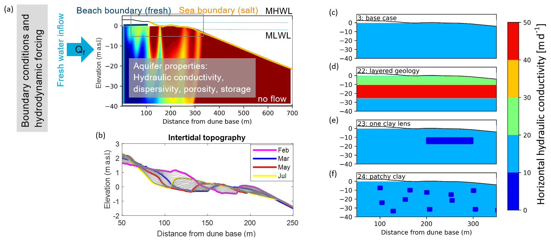
Figure 1 (a) Model setup with dimensions, boundary conditions, and parameters (colours indicate salt distribution: red is salty, blue is fresh). The thin grey box encompasses the part of the sea boundary where changes in beach morphology occur. (b) Four lidar scans (Grünenbaum et al., 2020a) of intertidal topography and interpolated topographies (grey lines in 10 d increments). Panels (c) to (f) show four different geological settings; note that K_h = 0.005 m d⁻¹ for the clay lens and clay patches (dark blue).

2.1 Model approach

Density-driven flow and transport were simulated with SEAWAT4 (Langevin et al., 2007), which couples the modules of groundwater flow MODFLOW 2000 (Harbaugh et al., 2000) and multispecies transport MT3DMS (Zheng and Wang, 1999). Model input and output were processed with the Python package FloPy (Bakker et al., 2016; USGS, 2021). To investigate the mixing-controlled reaction potential, a simple reaction model was implemented with PHT3D (Prommer and Post, 2010) that couples SEAWAT with PHREEQC (Parkhurst and Appelo, 1999).

The transient 2-D model representing a 700 m long cross-shore transect was discretized into 350 columns with a uniform horizontal length of 2 m and 80 layers with a thickness of 0.5 m each, except for the first layer. The top of the first layer was set to 3 $\mathrm{m}\mathrm{a}.\mathrm{s}.\mathrm{l}.$ at the upper beach and −0.1 $\mathrm{m}\mathrm{a}.\mathrm{s}.\mathrm{l}.$ in the intertidal zone to avoid re-wetting problems. The bottom of the first layer was set to −0.5 $\mathrm{m}\mathrm{a}.\mathrm{s}.\mathrm{l}.$ for all cells. The 2-D approach was justified since the groundwater flow is directed predominantly from the islands' freshwater lens towards the shoreline. The simulation period was 20 years with daily time steps. No-flow boundaries (Neumann type) were defined at the northern vertical sea boundary and at the aquifer base. Freshwater (Q_f) (salt concentration = 0 g L⁻¹) entering from the interior of the island (freshwater lens) along the southern vertical boundary was defined with a prescribed flux per unit coastline length of 0.5 m³ (dm)⁻¹ as estimated by Beck et al. (2017) and distributed uniformly across the cells of the first column (Fig. 1). Meteoric groundwater recharge of 400 mm a⁻¹ was applied at the upper beach above the MHWL. A general head boundary (GHB) with a high conductance of 1000 m² d⁻¹ was specified along the seaside and intertidal zone (Fig. 1) to ensure good aquifer connection. The hydraulic head of the GHB boundary was set to 0 below the MLWL. This approach helped avoid numerical issues that could arise from using a constant head boundary in a highly transient system, where boundary conditions might change due to shifts in beach morphology. In the intertidal zone (between the MLWL and the upper beach affected by storm floods) the beach surface was interpolated according to the methodology described by Greskowiak and Massmann (2021). Four cross-shore lidar scan profiles (as shown in Fig. 1b, obtained for March to July 2017 and February 2018) were sampled at 1 m resolution and interpolated to daily increments over a period of 6 months. The topography was then varied in daily increments for 6 months and reversed for the second half of the year. The resulting annual topography was applied recursively over the simulation for a period of 20 years. Daily topography time series were then used to calculate the hydraulic heads using the tide-averaged head approach, which were assigned to the sea boundary in the intertidal zone (Fig. 1a, grey box). Hereby, above the MLWL the tide-averaged approach (Vandenbohede and Lebbe, 2007) was applied and desaturation was accounted for by reducing the head by 17 cm (Greskowiak and Massmann, 2021) at the HWL and linearly decreasing to 0 cm at the MWL (Greskowiak and Massmann, 2021). Three storm surges were implemented by directly applying seawater recharge above the high tide mark for 1 d in each winter month, whereby water fluxes were calculated based on the thickness of the unsaturated zone multiplied by the porosity (Holt et al., 2019). In the intertidal zone at the GHB, saltwater inflow and outflow were modelled using nondispersive flux boundaries. A solute concentration of 35 g L⁻¹ was assigned to the inflowing saline water and the simulated concentration to the outflowing water. This third type of transport boundary condition transports solute mass out of the model domain based on the product of the discharging water and its respective solute concentration. The initial salt distribution was fresh (0 g L⁻¹) landwards from the MLWL and saline (35 g L⁻¹) seawards of it. Aquifer properties and boundary conditions are listed in Table 1.

2.1.1 Mixing-controlled reaction potential

Instead of modelling real mixing reactions, such as iron oxide precipitation at oxic–anoxic interfaces (Charette and Sholkovitz, 2002), we adapted the approach by Perez et al. (2023) and Valocchi et al. (2019), who used a hypothetical reaction potential where a solute C is produced by mixing of solutes A and B in different groundwater end members. Specifically, we considered a theoretical mixing scenario where two mobile reactants, Rf and Rs, entered the system via the freshwater and saltwater boundaries, respectively, and were transported with the groundwater through the STE. When they mixed, they produced the immobile mixing reaction product Mp via the following reaction rate formulation, which was implemented in the model using PHT3D:

$$\begin{array}{}\text{(1)}& r_{\text{Mp}}=\mathrm{d}\left[\text{Mp}\right]/\text{d}t=k\times \text{[Rf]}\times \text{[Rs]},\end{array}$$

where [Rs] is the concentration of the saltwater reactant Rs, [Rf] is the concentration of the freshwater reactant Rf, [Mp] is the concentration of the immobile mixing product Mp, k is the reaction rate constant, and r_Mp is the production rate of Mp. Note that Rf and Rs were not removed by this process and the formed Mp accumulated during the simulation period of 20 years. Hence, at the end of each simulation, Mp was a measure for the extent and intensity of the mixing-controlled reaction potential. Also note that the reaction rate constant was arbitrarily set to k = 10⁻⁷ $(\mathrm{mol}{\mathrm{L}}^{-\mathrm{1}}{)}^{-\mathrm{1}}{\mathrm{s}}^{-\mathrm{1}}$ for all simulation cases. As Rf and Rs were not removed by this processes, the relative differences of the mixing-controlled reaction potential between the different simulation cases are independent from the value of k. Thus the value of k has no further meaning, as long as it is greater than zero. The reaction network was implemented into the PHT3D modelling framework. The initial distribution of Rf and Rs, each with a concentration of 10⁻³ mol L⁻¹, was in line with the initial salt distribution with Rf present landwards from the MLWL and Rs seawards of it.

2.2 Model cases and case evaluation

A total of 24 different model cases were systematically tested covering six aquifer parameters (K_h, K_v, α_L, α_T, n, S_s) and three boundary conditions (beach recharge, freshwater inflow from the island (Q_f), number of storm floods). Each parameter was changed to significantly higher and lower values compared to the base case while still being in a realistic range for sandy STEs in a temperate climate (Table 1). Furthermore, cases with a stable beach morphology with and without storm floods (SFs) as well as with three different permeability distributions (Fig. 1c–f) were tested. All parameters and boundary conditions are listed in Table 1.

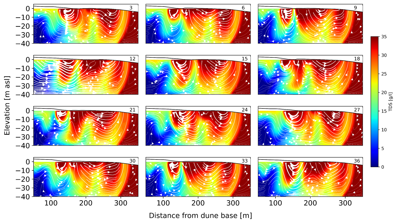
Figure 2 Cross-sections of TDS distribution (coloured areas) and flow field (white flow lines) for the base case, shown for every 3 months of the last 3 years of the simulation period. Thicker flow lines indicate higher flow velocities. The number in the right corner refers to the month.

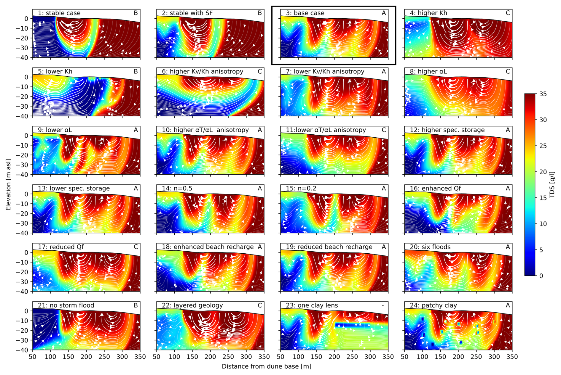
Figure 3 Snapshots of the flow regime (white flow lines) and salinity distribution (coloured areas) for the 24 model cases at the end of the 20-year-long simulation period. The base case is framed in black. Thicker flow lines indicate higher flow velocities. The letter in the upper right corner refers to the cluster group (see Table 1 and Fig. 6).

Figure 4 Standard deviation (SD) of TDS over the last 10 years of the simulation period for the 24 model cases. The base case is framed in black. The letter in the upper right corner refers to the cluster group (see Table 1 and Fig. 6).

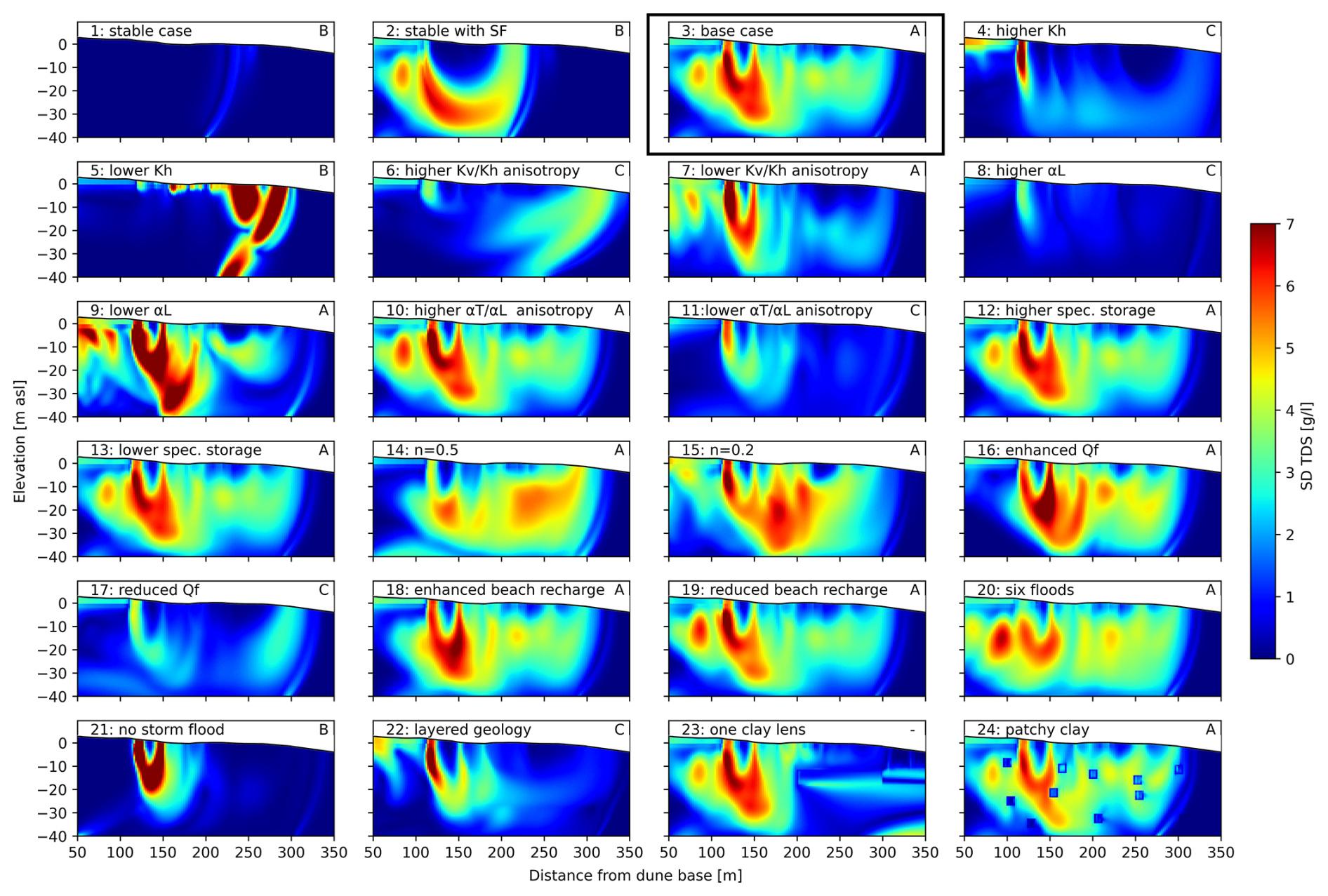
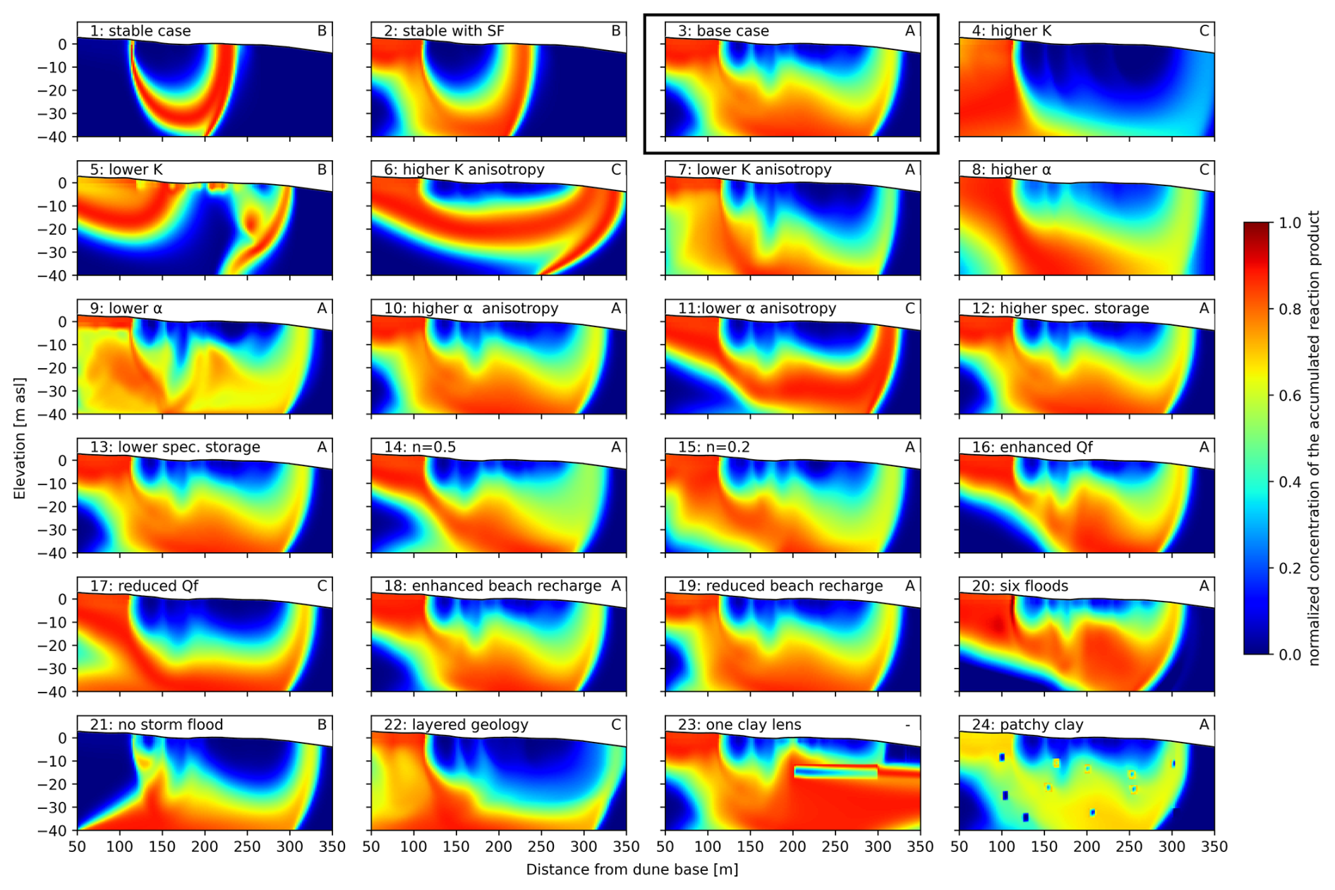
Figure 5 Normalized concentration of the accumulated reaction product (Mp) indicating the reaction potential for all 24 model cases over the last 10 years of the simulation period. The base case is framed in black. The letter in the upper right corner refers to the cluster group (see Table 1 and Fig. 6).

The model results were evaluated according to (1) the flow regime visualized as flow lines (Figs. 2 and 3), (2) the TDS distribution shown as snapshots at the end of the simulation (Fig. 3) as well as the standard deviation of the TDS concentration (SD) in each cell over the last 10 years of the simulation period (Fig. 4), and (3) the reaction potential RP_C (Eq. 2) normalized to the absolute maximum Mp_C concentration across all model cases (Fig. 5). Here, RP_C is the sum of the accumulated mixing products in each cell (Mp_C) over the last 10 years of the simulation period, calculated by subtracting the accumulated mixing concentration of the first 10 years from the final concentration at the end of the 20-year simulation period. The decision to evaluate SD TDS and RP_C based on the last 10 years of the simulation period was taken to avoid the potential influence of the initial distribution of TDS, R_s, and R_f. Therefore, the first 10 years of the simulation period serve as a model spin-up.

The reaction potential at each cell is

$$\begin{array}{}\text{(2)}& {\mathrm{RP}}_{\mathrm{C}}=\mathrm{\Sigma }{\mathrm{Mp}}_{\mathrm{C}}.\end{array}$$

The reaction potential in the entire model is

$$\begin{array}{}\text{(3)}& {\mathrm{RP}}_{\mathrm{M}}=\mathrm{\Sigma }{\mathrm{RP}}_{\mathrm{C}}.\end{array}$$

The indices C and M refer to cell and model, respectively.

To compare the variation in salinity (γ) of the different model cases the SD of each cell was summed up for each model case (SumSD_MC) divided by the number of cells (N) and normalized to the base case (SumSD_BC):

$$\begin{array}{}\text{(4)}& \mathit{\gamma }=\left[\right({\mathrm{SumSD}}_{\mathrm{MC}})/N]/\left[\right({\mathrm{SumSD}}_{\mathrm{BC}})/N].\end{array}$$

γ and RP_M (normalized to the base case) serve as a measure for the dynamic character of the system and were used in a k-means cluster analysis to group the 24 cases (Fig. 6).

3 Results

3.1 Base and stable cases

The model proposed by Greskowiak and Massmann (2021), which incorporates a transient beach morphology and three storm floods, was employed as the base case in the present study. Boundary conditions and aquifer parameters were then varied to identify their individual influence on flow and salt transport as well as mixing-controlled reaction potential. The results of the different model variants were compared to the base case.

In the stable case the average beach topography from the base case and no storm floods were considered.

The simulations were transient and hence the flow field and the salinity distribution varied over time in all models except the steady state of the stable case (case 1). This temporal development is exemplarily shown for the base case in Fig. 2.

Base case

The flow and salt dynamics in the base case (case 3) with a temporally varying topography and storm floods showed the formation of salt fingers and several USPs in front of the main USP moving through the subsurface. Consequently, salinities varied over time throughout the entire STE. Likewise, the flow velocities, flow directions, and discharge locations varied over time. Flow was enhanced and flow lines were more horizontal in times of storm floods (e.g. Fig. 2, month 12). Flow lines were more undulating in regions with stagnant water outside the storm season. The SD of TDS was highest below the area of the MHWL that moved along the transect due to dynamic topography (Fig. 4, case 3). The Mp concentration was high down to 10 $\mathrm{m}\mathrm{a}.\mathrm{s}.\mathrm{l}.$ below the storm-flood-affected area and deeper below the intertidal zone where the FDT and constantly moving USPs were mixing (Fig. 5, case 3). Compared to Greskowiak and Massmann (2021) the first layer was more finely discretized to better accommodate reactive transport, but the results in general showed the same flow and transport patterns.

Stable topography cases

A stable topography without storm floods (Fig. 3, case 1) led to the classical picture of a tidal STE (Robinson et al., 2006) with one USP, reaching down to 30 m, on top of a FDT that was pushed down by the infiltrating saltwater of the USP, discharging near the MLWL while being pushed upward by the circulating SW. As would be expected in the stable case, the SD (Fig. 4, case 1) was very low, close to 0, and mixing-controlled reactions took place along the fringes of the USP and the SW only (Fig. 5, case 1). Taking into account storm floods while maintaining a constant topography (case 2) led to changes of the flow regime and deformation of the USP (Fig. 3, case 2). At the same time, the reaction domain expanded and the mixing-controlled reaction potential increased below the storm-flood-affected area (Fig. 5, case 2), where SD was higher (Fig. 4, case 2) compared to case 1.

3.2 Impact of aquifer parameters

Hydraulic conductivity

A higher K (case 4) in this flux-driven system resulted in high infiltration rates of saltwater in the USP and freshwater from inland. The freshwater was forced to move upwards, partly recirculating in front of a large, relatively stable (low SD) saltwater body (Figs. 3 and 4, case 4). A FDT did not form and freshwater discharged near the MHWL. The recirculating brackish water in front of the saltwater body mixed constantly with inland freshwater and saltwater from the storm floods, resulting in an extensive zone with high reaction potential under the upper beach (Fig. 5, case 4). In contrast, a lower K (case 5) resulted in a widening of the FDT (Fig. 3, case 5). Saltwater was hindered from infiltrating, and both the SD and the RP were high close to the SW and in the upper part of the aquifer influenced by storm floods (Figs. 4 and 5, case 5). A higher K anisotropy (case 6) led to the establishment of a relatively stable, wide FDT with uniform flow, with overall low SD (Figs. 3 and 4, case 6). The high-RP zone was concentrated in the area affected by storm floods, the deeper USP, and the wedge interface (Fig. 5, case 6). On the other hand, a lower K anisotropy (case 7) distorted the flow regime and led to strong fingering flow (Fig. 3, case 7). The zone of SD was small and focused below the MHWL (Fig. 4, case 7), where the RP was also high (Fig. 5, case 7).

Dispersivity

The higher-α_L case (Fig. 3, case 8) resembled the higher-K case (Fig. 3, case 4). The higher dispersivity led to more mixing (wider zone of RP), and one big relatively stable dispersed USP formed (Figs. 4 and 5, case 8). The FDT became more brackish and less distinct. The SD was generally low and the RP was large in the area bordering the USP and also much larger than in the high-K case (case 4). A lower α_L (case 9) led to sharper contrasts between saline and freshwater bodies with wider mixing zones but with lower Mp concentrations (Figs. 3–5, case 9).

A higher α anisotropy (α_T/α_L) (case 10) had only a minor impact on the flow and transport patterns compared to the base case (Figs. 3 and 4, case 10), except for a slightly more dispersed RP zone (Fig. 5, case 10). A lower α anisotropy (α_T/α_L) (case 11) produced a more uniform flow regime below the upper beach, with relatively stable TDS patterns indicated by a small and focused SD (Figs. 3 and 4, case 11) and a smaller, more focused RP zone along the fringe of the USP (Fig. 5, case 11).

Specific storage

The variation in S_s (cases 12 and 13) basically had no effect compared to the base case (Figs. 3–5, cases 12 and 13).

Porosity

A higher porosity (case 14) increased the effective flow-through area and reduced flow velocities (Fig. 3, case 14). Consequently, residence times were prolonged and hence the entire system was less mixed, as indicated by smaller SDs (Fig. 4, case 14). RP was only slightly reduced compared to the base case (Fig. 5, case 14) because a reduction of mixing reduced the formation of MP but longer residence times enhanced the formation of MP. A reduction in porosity (case 15) had the opposite effect; i.e. less pore space caused faster flow-through, decreased residence times, and enhanced mixing, as indicated by higher SDs and only slightly enhanced RP (Figs. 3–5, case 14).

3.3 Impact of boundary conditions

Freshwater inflow

Enhanced inflow from the inland freshwater boundary (case 16) had a freshening effect and resulted in a more uniform flow regime below the upper beach with higher TDS variation and a narrower RP zone, while the SD was more pronounced around the MHWL (Figs. 3–5, case 16). A reduction in freshwater inflow (case 17) made the system more brackish (Fig. 3, case 17), resulted in less SD (Fig. 4, case 17), and caused a wider RP zone (Fig. 5, case 17).

Beach recharge

A variation in fresh beach recharge (cases 18 and 19) showed effects mostly landwards of the USP below the storm-flood-affected upper beach. A higher beach recharge (case 18) led to stronger dilution of saltwater that previously infiltrated during storm flood events due to the higher groundwater recharge (Fig. 3, case 18). The SD was smaller than in the base case below the upper beach caused by the enhanced mixing, resulting in constantly brackish water (Fig. 4, case 18). Reduced beach recharge (case 19) in turn showed sharper (higher concentration gradients) saltwater fronts from storm flood events, which did, however, reach less deep (Fig. 3, case 19). The SD was higher in the shallow part of the upper beach, caused by the downward-moving sharper saltwater fronts (Fig. 4, case 19). While the overall RP was less affected by the variation in beach recharge compared to the base case, small differences were visible below the upper beach: more focused RP for enhanced recharge and less pronounced RP for reduced recharge, yet impacting a larger area (Fig. 5, cases 18 and 19).

Storm floods

Doubling the number and frequency of the storm floods (case 20) in comparison to the base case enhanced the saltwater flux through the upper beach (Fig. 3, case 20). TDS increased, as did the SDs (Figs. 3 and 4, case 20), and the zone of higher RP reached further down below the upper beach (Fig. 5, case 20). Without storm floods (case 21) the system dynamics were driven only by the continuously changing topography, resulting in a movement of the intertidal zone and the USP across the shore (Fig. 3, case 21). The SDs were highest in the USP around the MHWL (Figs. 3 and 4, case 21). The zone of high RP was restricted to the lower part of the aquifer, rising up below the MHWL (Fig. 5, case 21).

Geological structure

A layered geology (case 22) (alternating permeable sand layers) led to more mixing and dilution below the upper beach (Figs. 3 and 4, case 22). The SDs were comparatively small and restricted to the MHWL. The high-RP zone was wider below the upper beach and covered the entire aquifer thickness, while it was restricted to the lower part of the aquifer below the intertidal zone.

A single, extensive clay lens (case 23) made a significant difference for the entire flow regime. On the landward side, the first 200 m of the subsurface looked similar to the base case (Fig. 3, case 23). In the vicinity of the clay layer, several smaller USPs were restricted to the area above the clay layer, while flow was rather uniform below the clay layer. The SW was shifted further offshore (not visible in Fig. 3). The salt fingers moving towards the clay layer from onshore were distorted by the clay layer. The SDs were high below the upper part of the intertidal zone (Fig. 4, case 23) and the zone with high RP extended offshore (Fig. 5, case 23).

Patchy small clay lenses (case 24) distributed throughout the STE led to only small and very local deviations of groundwater flow and salinity patterns as well as local changes in SDs and RPs around the clay patches (Figs. 3–5, case 24), while the overall picture was very similar to the base case.

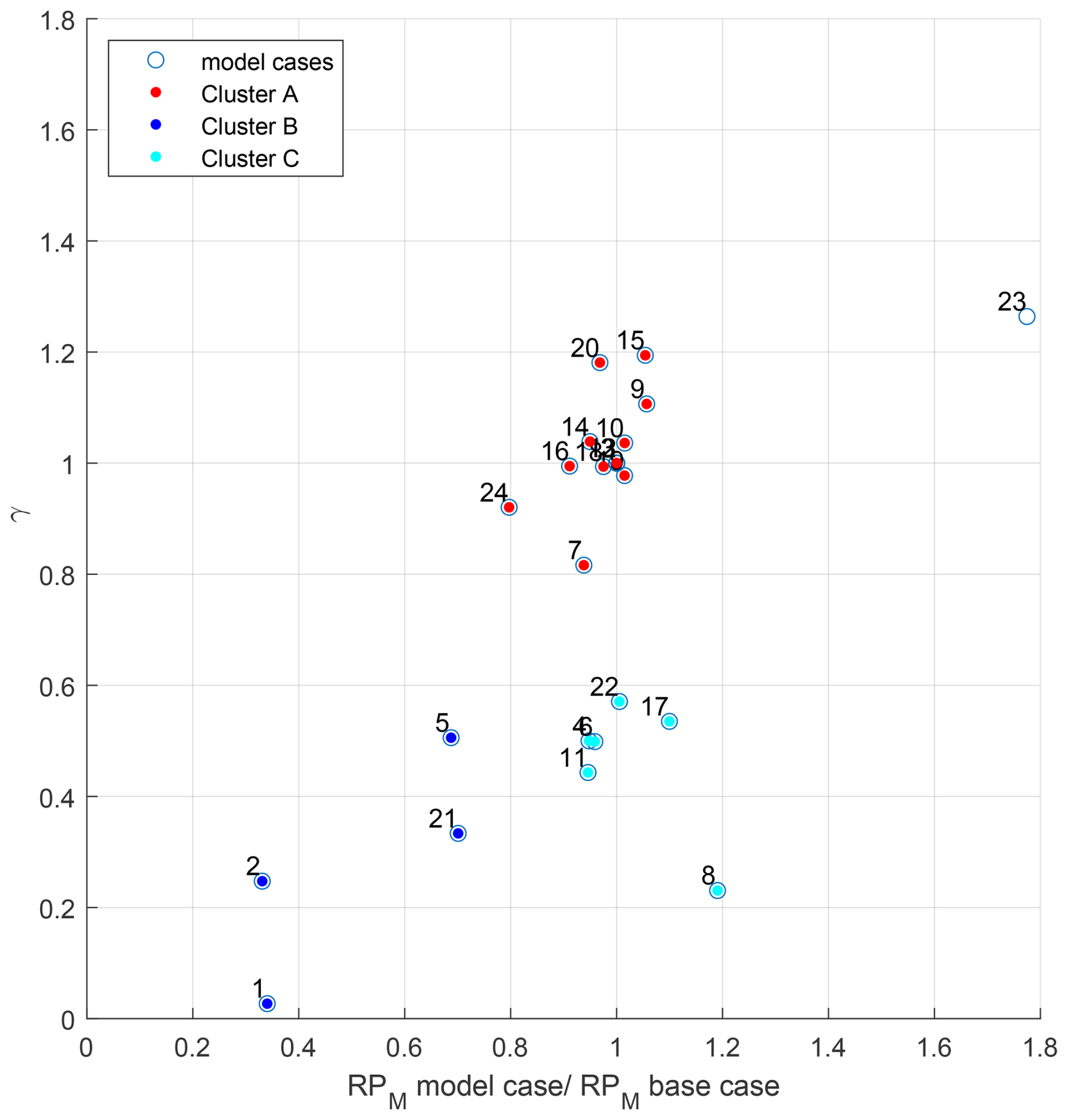
Figure 6 Cluster analysis (k-means, 3) of all model cases based on model variation in salinity (γ) and the sum of the reaction product of each model (RP_M). Individual model values were normalized to the base case (located at 1,1 in the plot).

3.4 Cluster analysis

A k-means analysis based on γ and RP_M of each model case normalized to the same statistics of the base case resulted in the clustering of the model cases into three main groups (Fig. 6, Table 1). Cluster A (red circles) was characterized by relatively small variations of γ and RP_M with respect to the base case, namely variations in the range from −20 % to +20 %. In Fig. 6, the base case corresponds to the point with coordinates (1,1). Cluster B (dark blue circles) showed a lower γ, reduced by more than 40 %, and a lower RP_M, reduced by more than 30 %, compared to the base case. Cluster B contained the less dynamic and more stable cases with either changing topography only (and no storm floods, case 21), only storm floods (and no changing topography, case 2), or neither (case 1) and the low-K case (case 5). Cluster C (light blue circles) was characterized by values of γ reduced by more than 40 %, while RP_M remained close to the base case (variations in the range from −20 % to +20 %). One outlier, case 23 with one clay layer, showed a significantly higher γ and higher RP_M compared to the base case.

4 Discussion

The purpose of this study was to identify the main drivers of the flow and transport dynamics in the subsurface of a high-energy beach by systematically changing aquifer parameters and boundary conditions, thereby evaluating their individual effect on the flow and transport regime as well as mixing-controlled reaction potential. Conditions and parameters chosen are realistic for the barrier island Spiekeroog, which is representative for a high-energy STE. We found that results are most sensitive to a variable beach morphology, storm floods, hydraulic conductivities, and dispersivity.

4.1 Flow and transport regime

A temporally changing morphology led to the constant migration of the MHWL and MLWL on the beach transect. The intertidal zone width varied, as do the USP and the discharge zones. This behaviour has previously been observed in field studies targeting the shallow subsurface on Spiekeroog (Grünenbaum et al., 2020a; Waska et al., 2019). The findings of the present study indicate that constantly changing infiltration and exfiltration locations cause the onset of instable conditions that also drive the dynamics in the deep subsurface. Additionally, the beach surface, which is sometimes straight and at other times forms a berm–trough system (Grünenbaum et al., 2020a) due to sediment erosion–accretion, affects groundwater flow and salt transport as well as the mixing-controlled reactions. This dynamic upper boundary results in flow paths and flow velocities that vary continuously, thereby enhance mixing in the subsurface. The seasonal storm flood events add saltwater to the upper beach, which, together with the changing morphology, acts as an effective pump pushing the saltwater, FDT, and several USPs through the intertidal zone.

4.2 Mixing-controlled reaction potential

The dynamic groundwater flow and transport in the STE trigger mixing-controlled reactions. Anwar et al. (2014) found that oceanic forcing increases the freshwater–seawater mixing, enhancing nutrient transformation. Heiss et al. (2017) concluded that mixing-dependent processes are positively correlated with the size of the USP that in turn is affected by oceanic forcing and hydrogeological parameters. Our results show that in particular the dynamic beach morphology and the storm floods drive subsurface flow and transport dynamics and result in changes of the location, shape, extent, and intensity of what we refer to as the mixing-controlled reaction potential. Similarly, Greskowiak et al. (2023) concluded that a dynamic beach morphology and storm floods were the main factors effecting redox zones in the deep STE, which, however, are largely a function of travel time rather than mixing.

4.3 Synthesis of the 24 model cases

We found that in addition to morphodynamics and storm floods, the horizontal and vertical hydraulic conductivity and longitudinal and transverse dispersivity significantly influence the shape, location, stability, and extent of the USP, FDT, and mixing-controlled reactions. However, our results also suggest that some factors only control the flow and transport regime but not the reaction potential in the same way. For example, a higher longitudinal dispersivity (case 8) and a reduction in freshwater inflow (case 17) caused a significantly reduced SD (Fig. 4), while the RP shows an overall similar shape compared to the base case (Fig. 5).

Three main groups were identified in the k-means cluster analysis that best characterize the overall system behaviour as either similar to the base case (cluster A), resulting in less variable salt patterns and less reactive conditions than the base case (cluster B), or resulting in less variable salt patterns but similar reactive conditions compared to the base case (cluster C). Changing the values of hydraulic conductivity or dispersivity and their respective anisotropies caused the model cases to end up in different clusters. Hence, subsurface dynamics are particularly sensitive to these parameters. Also, geological structures with a high K contrast may strongly change flow, transport, and mixing in the STE if they are large enough, as exemplarily shown for case 23 with one large clay lens in the intertidal zone. Other parameters and boundaries or small-scale geological heterogeneities hardly affected the system but are still important to take into account when building site-specific models of STEs evaluated based on point observations.

4.4 Study limitations

Our generic modelling approach has some limitations. We used a 2-D setup as did former studies at Spiekeroog (Beck et al., 2017; Greskowiak and Massmann, 2021; Grünenbaum et al., 2020b; Röper et al., 2012) as well as at other sites (Anwar et al., 2014; Heiss et al., 2017; Michael et al., 2016; Robinson et al., 2006). However, as our results show that morphological changes have a major impact on the salt distribution, and considering that the beach morphology and associated head gradients are variable along the shore (Geng and Michael, 2021; Knight et al., 2021; Paldor et al., 2022; Reckhardt et al., 2024), the subsurface flow in the STE is likely characterized by a 3-D flow component. Moreover, we used a measured, but linearly interpolated, variable beach topography. In reality, rapid changes in morphology are likely to occur caused by short-term events (Karunarathna et al., 2018) such as storm floods or strong winds and consequently enhance the dynamics in the subsurface. Further, repeatedly changing the morphology over an annual cycle leads to cyclic groundwater flow and salt transport patterns, but in a real-world system the changes will be less regular.

The location of the beach boundary, to which freshwater inflow is assigned, is in close proximity to where flow, transport, and mixing variations occur. Consequently, it is likely to exert a boundary effect where increased freshwater inflow reduces TDS concentrations. Conversely, if the boundary were to lie further inland, TDS concentrations below the upper beach would be enhanced, as water is allowed to flow further inland during possible flow reversals. However, this only happens during extreme storm flood events, and as these are infrequent and short lived (1–2 d), there is not enough time for additional salt to accumulate as a result of the flow reversal. Furthermore, as this only occurs along the southern vertical boundary of the models, we expect it to have an insignificant effect on the overall flow, transport, and mixing patterns in the intertidal zone. In our generic modelling approach, we systematically changed single aquifer parameters and boundary conditions, though some of these parameters may be correlated. At the same time, boundary conditions can be inter-dependent or affected by seasons. We chose this approach to better disentangle single effects and refrain from analysing combined cases.

To optimize the numerical effort with a daily time stepping we neglected waves and used the tide-averaged approach as did e.g. Vandenbohede and Lebbe (2007). However, previous studies showed that wave- and tide-resolved approaches intensify freshwater–saltwater mixing, resulting in enhanced nutrient transformation and the discharge of nutrients from the land to the sea (Anwar et al., 2014; Heiss et al., 2017). The use of a tide-averaged approach is also the reason why the change in storage parameters does not show any impact on groundwater flow and transport that would be expected in a real-world system. As demonstrated by Grünenbaum et al. (2020b), the effect is rather small on salinity and travel time distributions as tides produce only very small back-and-forth displacements of groundwater parcels within a tidal cycle, but it broadens the transition zone. We systematically started with a homogenous geology and showed a layered case and one with a thick clay lens and smaller clay patches instead of using statistically generated heterogeneities as done by Michael et al. (2016). The heterogeneous distribution of other aquifer parameters, e.g. porosity (Meyer et al., 2018a), might also be of relevance but was neglected here.

5 Conclusion

This study aimed to advance the understanding of flow and transport processes in STEs under high-energy conditions. We systematically investigated the interplay of morphological changes and hydrodynamic boundary conditions paired with aquifer properties of a high-energy beach in a 2-D generic modelling approach with 24 model cases. Except for the stable case (case 1), which disregards morphodynamics and storm floods, groundwater flow and salt transport were highly dynamic, thereby enhancing mixing-controlled reactions. The main factors controlling the subsurface dynamics were the changing beach morphology, storm floods, hydraulic conductivity, and dispersivity as well as major geological structures. The results highlight the need to account for the changing topography and storm floods when studying and modelling high-energy beaches. Moreover, good knowledge of the geological structures and parameter estimates is necessary. The flow and transport regimes are coupled to mixing-controlled reactions and hence transformation of nutrients in the subsurface. If disregarded, resulting net fluxes to and from the sea might be overestimated or underestimated.

In the future, extending the model domain to 3-D while also accounting for morphodynamics could help to assess to what extent subsurface flow is three-dimensional under high-energy conditions. The implementation of real data, including high-resolution beach topography, such as those currently being collected from a beach observatory on Spiekeroog (Massmann et al., 2023), in model calibration will further help to better constrain and understand the biogeochemical functioning of high-energy STEs. Here, we studied the extent of mixing-controlled reactions in the subsurface with a simplified hypothetical reaction model. To move on to further study and quantify in situ biogeochemistry in the STE, reactive transport modelling approaches targeting real-world reactions would be a valuable step forward.