Exploring the driving factors of compound flood severity in coastal cities: a comprehensive analytical approach

Coastal cities face severe compound flooding, including both fluvial flooding and pluvial flooding. Currently, there is a lack of comprehensive methods to analyze the driving factors of compound flooding. This study establishes a coupled one-dimensional and two-dimensional hydrodynamic model. Based on historical data, the model constructs joint probability distributions of rainfall and tide levels with different return periods and durations. Using the results from the coupled model under various design scenarios, the study proposes an impact index to quantify the relative contributions of rainfall and tide level to flooding. Additionally, the model quantifies the interactions between fluvial flooding and pluvial flooding. Taking the Shahe River basin in Guangzhou, China, as a case study, the results show that the combination of the copula function and the Kendall return period method is effective for designing hydrological variable combinations. The impact degree index of rainfall on flooding varies between 0.5 and 1, with the minimum at 24 h duration, indicating that the compound flooding is primarily affected by rainfall, and the influence of tide level is most significant at 24 h duration. The pluvial flooding caused by the influence of river water level on the drainage outfalls accounts for up to 19.08 % of the total volume. This shows that fluvial flooding affects the seriousness of compound flooding by influencing the water levels of outfalls. The flood-prone area is divided into different regions based on the main natural factors (rainfall and tide level) and social factors (pipeline network, drainage outfalls, and riverbank defenses) to help decision-makers identify the causes of flooding in each drainage unit and better formulate targeted disaster-reduction strategies to improve flood control capabilities.

1 Introduction

The sixth assessment report by the Intergovernmental Panel on Climate Change (IPCC), released in 2021, predicts that heavy rainfall and floods will intensify and occur more frequently in many regions worldwide in the 21st century (Masson-Delmotte et al., 2021). This trend is already apparent in several countries, posing a significant threat to nations and their populations. For example, in 2023, severe rainstorms in February led to significant casualties in the state of São Paulo, Brazil (Marengo et al., 2024). In May, the Emilia-Romagna region in northern Italy was hit by heavy rainfall, resulting in at least 14 fatalities and 305 landslides (Dorrington et al., 2024). In July, both Pakistan and China experienced severe rainstorms and flood disasters (Jiao et al., 2024). The direct cause of these disasters was heavy rainfall. When the intensity of rainfall is high and its duration is prolonged, urban surface and underground drainage systems often struggle to handle such a large volume of water. Coastal areas also face the threat of tide levels, such as the southeastern coastal regions of China and the eastern coast of the United States. Tide levels not only include astronomical tides but also are influenced by meteorological tides, with storm surges being an extreme form of meteorological tides. When the tide level rises, it affects drainage capacity, and in more severe cases, this high level may lead to seawater backflow into the city, further exacerbating urban flood risks.

To better understand the flood risks caused by compound events of heavy rainfall and tide levels, researchers have focused on exploring the interdependence of various factors in the fields of hydrology, meteorology, and oceanography using copula theory (Pappadà et al., 2018; Zellou and Rahali, 2019). Wahl et al. (2015) analyzed the likelihood of compound events of storm surges and heavy rainfall occurring in coastal areas of the United States, and the results showed higher flood risk in the US east coast and gulf coast areas. Yang and Qian (2019) proposed using the particle swarm optimization (PSO) algorithm to estimate the marginal cumulative distribution of wind speed, storm surges, and heavy rainfall, as well as the parameters of the three-variable joint function. Latif and Simonovic (2022) combined rainfall, storm surges, and river discharge observations to create a three-variable probability framework.

Combining joint distribution models with return periods allows for the design of multivariate combination scenarios under different return periods. Extensive research studies have focused on identifying flood risks under various combinations of variables. Urban flood models are powerful tools for supporting these studies (van Dijk et al., 2013). While methods tend to evolve towards artificial intelligence algorithms, coupled one-dimensional and two-dimensional numerical models with interpretable physical processes remain popular. Zhang et al. (2022) designed rainfall scenarios under different return periods and compared urban flooding results under different rainfall scenarios using the MIKE FLOOD model. Lian et al. (2013) evaluated the combined impact of rainfall and tide levels on flood risk in coastal cities and found that the greatest threat comes from heavy rainfall, with tide levels adding additional flood risk. However, these studies did not quantify the degree of impact of rainfall and tide levels on flooding. Lian et al. (2017) proposed a method to divide the flood-prone area into three regions based on the magnitude of their impact, namely, rainfall area, tidal area, and common area. The common area is defined as the region where flooding is influenced by both tides and rainfall. The study used daily rainfall and daily tide levels but did not consider the effect of duration. In urban environments, short-duration heavy rainfall events are more likely to occur, making it particularly important to study the differential effects of rainfall and tide levels on flooding under different durations.

Urban flooding encompasses both fluvial flooding, which results from inadequate river capacity, and pluvial flooding, which occurs due to inadequate drainage in urban infrastructure. In underdeveloped areas, fluvial flooding is more common due to natural topography and a lack of infrastructure. With the development of urbanization, the increase in impervious surfaces has intensified the drainage pressure, making pluvial flooding more prominent. Therefore, urban flooding is the result of the combined effects of natural factors (such as rainfall and tide levels) and social factors (such as urban drainage systems and land use). Skougaard Kaspersen et al. (2017) compared the impact of climate change and urban development patterns on the exposure of four European cities to floods. Pervin et al. (2019) analyzed the impact of improving drainage infrastructure and proper solid-waste management on reducing urban flood risk. Huang et al. (2018) categorized the causes of flooding in Guangzhou, China, into two types: low-lying terrain and inadequate drainage facilities. These studies provide valuable insights for developing flood prevention and mitigation measures. However, they tend to combine fluvial flooding and pluvial flooding into a single category. As a result, there may be a lack of comprehensive understanding of the mechanisms of interaction between fluvial flooding and pluvial flooding. Fluvial flooding and pluvial flooding have distinct definitions but are closely related and can transform under certain conditions. For example, if upstream efforts increase drainage capacity, this may lead to increased downstream flood flow, thereby increasing the risk of exacerbating downstream fluvial flood disasters. On the other hand, if the river maintains high water levels continuously (even without levee breaches), it may result in drainage difficulties due to floodwater overtopping the outfall. This can worsen pluvial flooding. There are few research studies on the interactions between different types of flooding. This complexity and diversity make flood problems more challenging. To address flood problems, it is necessary to study the influence of natural factors on flooding and the interaction of different types of flooding.

The purpose of this study is to propose a universal method for enhancing our understanding of the risk and interactions of different types of floods under the combined impact of rainfall and tide levels, as well as to identify the driving factors of compound flooding. Section 2 introduces the study area, the Shahe River basin in Guangzhou, China, and provides information on data availability. Section 3 constructs and validates the stormwater flood model and describes the processes of bivariate joint distribution, impact degree index, and spatial interaction forces. Section 4 explores different combinations of scenarios with different rainfall and tide level conditions, analyzes the relative contribution of different-duration rainfall and tide level conditions on compound flooding, examines the interaction process between fluvial flooding and pluvial flooding, and identifies the causes of flooding in drainage units (DUs). Section 5 discusses the driving factors of compound flooding and the limitations of the study. Finally, Sect. 6 draws the conclusions. The study results can support the development of precise flood prevention and control for different types of floods.

2 Study area and data

2.1 Study area

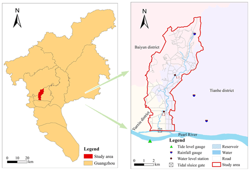
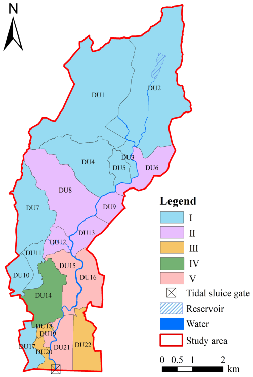
The Shahe River basin covers the Tianhe, Yuexiu, and Baiyun districts of Guangzhou, China, with a total area of 36.77 km². In this area, 63 % of the land is covered with hard surfaces, and only 1.2 % is water surface. The main river, the Shahe River, flows southward into the Pearl River. There is a small reservoir named Pachili in the area, with a catchment area of 2.04 km² and a total capacity of 1.44×10⁴ m³. This region receives abundant rainfall, with an average annual precipitation of 1676 mm, 81 % of which occurs between April and September. Urban flooding occurs frequently. Part of the reason is that the river and drainage network are affected by the tides of the Pearl River, which hinders the normal discharge of stormwater. The tides of the Pearl River are influenced not only by astronomical tides but also significantly by storm surges and upstream river flood flows. A tidal sluice gate, 24 m wide, has been constructed at the mouth of the Shahe River. However, no drainage pump station has been built, which creates significant drainage pressure during high-tide periods. The geographical location is shown in Fig. 1.

Figure 1 Location of the study area.

2.2 Data sources

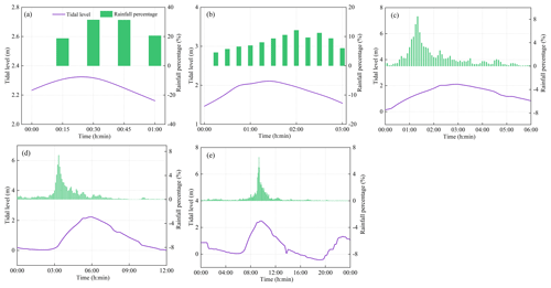
This study utilized rainfall data at 15 min intervals and tide level data at 5 min intervals from 2006 to 2021 for a rainfall–tide scenario design. Both rainfall and tide level data are gauge data. There are three rainfall gauges and one tide level gauge, as shown in Fig. 1. It is assumed that the rainfall distribution in the study area is uniform, and the rainfall data are averaged from the three gauges. The tide level data reflect the combined effects of astronomical tides, storm surges, and river flows. During Typhoon Mangkhut in 2018, the tide level gauge in this study recorded the highest tide level (3.28 m). DEM data (with a spatial resolution of 5 m), land use data, drainage network system data, river section data, and hydraulic engineering parameters were used for constructing the urban flood model. Measured rainfall, water level data, and water depth data on 23 May 2023 were used for model calibration. The topographic data were sourced from the Guangzhou Municipal Planning and Natural Resources Bureau, while other data were provided by the Guangzhou Water Authority.

3 Methods

3.1 Framework

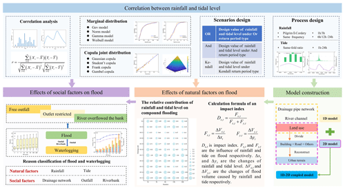
In this study, copula functions are used to construct combinations of rainfall and tide level scenarios with different durations. The Pilgrim–Cordery method and the same-frequency method were employed to design short-duration and long-duration rainfall events, respectively, while the modified equal–multiple method was used to design tide level processes. A coupled one-dimensional and two-dimensional hydrodynamic model based on the topography data was established to simulate the flooding under different scenarios. Subsequently, the impact degree index was proposed to quantify the relative contributions of rainfall and tide levels to flooding, and the differences in various drainage units for different durations were analyzed. Key time nodes were identified when river water levels exceeded the elevations of drainage outfalls and riverbanks, and flood volume and impact degree indices were calculated in stages to identify the interactions between fluvial flooding and pluvial flooding. Finally, the compound flood driving factors for each drainage unit were identified. This study aims to provide a scientific basis for formulating targeted compound flood management measures. The research framework is shown in Fig. 2.

Figure 2 Research framework diagram.

3.2 Combination design of rainfall and tide level

To further investigate the influence of rainfall and tide levels on compound flooding, this study establishes the joint distribution functions of rainfall and tide levels through correlation analysis. By utilizing Kendall return periods, various return periods of rainfall and tide levels are determined to simulate urban flooding. The designed return periods (RPs) include 2, 3, 5, 10, 20, 50, 100, and 200 years. Rainfall durations include 1, 3, 6, 12, and 24 h. Correlations are obtained by calculating the correlation coefficients between daily total rainfall and the highest tide levels from 2006 to 2021, including Pearson, Kendall, and Spearman correlation coefficients (Shaqiri et al., 2023).

3.2.1 Joint distribution of rainfall and tide levels

This study selects samples for joint distribution from rainfall and tide level data spanning 2006 to 2021. First, the annual maximum rainfall is calculated each year to form set D, with the minimum value in set D serving as the sample threshold. Subsequently, events from the 16-year historical data that are greater than or equal to this threshold are selected as preliminary rainfall samples. During sample selection, if the dry period between two samples is less than 6 h, the sample with the larger rainfall is chosen. Additionally, for multiple events exceeding the threshold on the same day, only the event with the maximum rainfall is retained, resulting in the final rainfall sample. For each selected rainfall sample, the highest tide level value on the same day is identified as the tide level sample. The rainfall thresholds corresponding to durations of 1, 3, 6, 12, and 24 h are 36, 56, 58, 66, and 78 mm, respectively. The final sample sizes are 48, 39, 49, 49, and 52, respectively.

Based on the above sample data, joint distributions of rainfall and tide levels for different durations are established. First, the generalized extreme value (GEV) distribution, normal (Norm) distribution, gamma distribution, and Weibull distribution are applied to estimate the marginal distributions for rainfall and tide level separately. It should be noted that the lower limit of the gamma distribution is 0. Then, two-dimensional Gaussian copula, Student's t copula, Frank copula, and Gumbel copula are constructed to fit the best-fitting marginal distributions, generating the joint distributions for rainfall and tide levels (Li et al., 2023). Based on the optimal joint distribution, the joint probability of rainfall and tide levels is calculated. Both marginal and joint distributions are estimated using the maximum likelihood method to estimate their parameters (Gibson et al., 2005). The fitting effectiveness is evaluated using the Akaike information criterion (AIC) method as the main criterion, along with the root-mean-square error (RMSE) and the Bayesian information criterion (BIC) method (Zhang and Singh, 2006). The Kolmogorov–Smirnov (K–S) test is used to verify the reasonableness of the results (Kavianpour et al., 2018).

3.2.2 Joint risk probability analysis

Univariate return periods estimate the probability of a hydrological variable exceeding a threshold within a given time frame. For multiple variables, “And” return period and “Or” return period types are commonly used. The “And” return period narrows the danger zone, while the “Or” return period expands it (Fig. S1 in the Supplement). To address this issue, Salvadori and De Michele (2010) introduced the concept of Kendall return periods. They defined a boundary, represented by a curve C(u,v)=p, for events with the same copula value. This boundary divides the event domain into safe and dangerous areas (Fig. S1). The essential difference from other return periods is that a series of events with the same return period is represented by a single value, which aligns more closely with real-world conditions.

In the case of the bivariate joint distribution, the design value corresponding to a specific return period is composed of numerous variable combinations. Among these combinations, there is always one that maximizes the joint probability density. Once this combination is identified, the design values for rainfall and tide levels are computed using the inverse functions of the optimal marginal distributions.

3.2.3 Design of the combined rainfall and tide events

For short durations (1 and 3 h), the Pilgrim–Cordery rainfall model is used to construct the rainfall processes (Pilgrim and Cordery, 1975). For longer durations (6, 12, and 24 h), the designed rainfall processes are derived using the same-frequency method, referencing the outcomes of the “Technical Report on the Compilation of Guangzhou Rainstorm Intensity Formula and Design Rainfall Patterns” for calculations. The tide level on 22 May 2020 is selected as the typical tide level process, according to the “Comprehensive Planning for Drainage (Rainwater) and Waterlogging Prevention in Guangzhou (2022–2035)” document. The typical tide level process is modified using an equal-ratio amplification method to design the tide level process. More details are provided in Sect. S1 in the Supplement. When the rainfall duration is 24 h, the designed tide level shares the same start and end times as the designed rainfall. For rainfall durations of 1, 3, 6, and 12 h, the peak tide level is set at the midpoint of the rainfall duration.

3.3 Model construction and verification

3.3.1 Model construction

In this study, a coupled one-dimensional (1D) and two-dimensional (2D) hydrodynamic model is constructed to study the response of urban flooding to different rainstorm and tide level scenarios. The 1D hydrodynamic model consists of the urban drainage network model and the 1D river model. It utilizes the Saint-Venant equations to perform calculations. The governing equations are expressed as follows:

$$\begin{array}{}\text{(1)}& {\displaystyle \frac{\partial A}{\partial t}}+{\displaystyle \frac{\partial Q}{\partial x}}=\mathrm{0},\end{array}$$

$$\begin{array}{}\text{(2)}& {\displaystyle \frac{\partial Q}{\partial t}}+{\displaystyle \frac{\partial }{\partial X}}\left({\displaystyle \frac{Q^{\mathrm{2}}}{A}}\right)+gA\left({\displaystyle \frac{\partial Z}{\partial X}}+S_{\mathrm{f}}\right)=\mathrm{0},\end{array}$$

where x is the distance (m), t is the time (s), Q is the volumetric flow rate (m³ s⁻¹), A is the flow area (m²), g is the acceleration of gravity (m s⁻²), and S_f is the friction slope.

The 2D hydrodynamic model adopts the 2D shallow water equations, i.e., the depth-averaged Navier–Stokes equations, to mathematically describe the 2D flow dynamics. It assumes that water flow primarily occurs in the horizontal direction, while variations in flow velocity occurring in the vertical direction are neglected. The storage cell method is used to solve the equation. For more details, our previous research results can be referenced (Wei et al., 2023). The governing equation can be represented as follows:

$$\begin{array}{}\text{(3)}& {\displaystyle \frac{\partial \mathit{\eta }}{\partial t}}+{\displaystyle \frac{\partial \mathit{\theta }}{\partial X}}+{\displaystyle \frac{\partial \mathit{\phi }}{\partial Y}}+S_{\mathrm{b}}+S_{\mathrm{f}}=\mathrm{0},\end{array}$$

where X and Y are the spatial coordinates; t is the time (s); θ and φ are the convective flux variables in the X and Y directions, respectively; S_b and S_f represent the source terms due to the slope of the terrain and the bed friction, respectively; and η is the conservation variable.

The tidal sluice gate is set to use tide levels as boundary conditions for outflow, ensuring that the model accounts for tide effects. The gate is opened when the water level inside the gate is higher than the level outside. The gate status is checked every hour and adjusted if necessary. To improve the representation of terrain data on roads and the abrupt vertical changes, the study area is divided into three parts: roads, buildings, and other features. Within the road area, elevation measurement points are used as references for nearest-neighbor interpolation. In the building area, vertical adjustments are made to the DEM data to reconstruct the terrain. This approach is based on the research by Huang et al. (2023), and the results of the model construction are shown in Fig. S2.

3.3.2 Model verification

Based on different land use types (Fig. S2), infiltration parameters for different catchment areas were preliminarily calibrated using the weighted average method. Characteristic parameters of each catchment and Manning's coefficients were set according to the existing research (Rossman, 2004). Then, observation data of the rainfall event on 23 May 2023 were used to calibrate the model. The main adjustment was made to Manning's coefficients of the channels, which were adjusted to values between 0.013 and 0.020. The Nash–Sutcliffe efficiency coefficients of the observed and simulated water levels at L1 and L2 (Fig. S2) were 0.79 and 0.89, with relative errors of 0.70 % and 0.26 % in the peak water depth. The error in peak appearance time was 15 min in both cases. The model verification results show that the stormwater flood model is suitable for subsequent research. The comparison between the measured water level and simulated water level is shown in Fig. S3.

3.4 Impact index of rainfall and tide levels on compound flooding

To quantify the relative contributions of rainfall and tide levels to compound flooding, this study introduces the impact index of rainfall on flooding and the impact index of tide levels on flooding. The severity of flooding is typically characterized by indicators such as flood volume, flood area, and flood depth. Within a given area, flood volume, as the product of flood area and flood depth, provides a more comprehensive measure. Therefore, in calculating the impact index, flood volume is used to represent flood severity.

The impact index of rainfall on flooding (D_x,t) is calculated by comparing the impact of rainfall on flooding with the total impact of both rainfall and tide levels, as shown in Eq. (4). Similarly, the impact index of tide levels on flooding (D_y,t) is calculated by comparing the impact of tide levels on flooding with the total impact of both rainfall and tide levels, as shown in Eq. (5). In this study, the impact index of tide levels on flooding can also be calculated as $\mathrm{1}-D_{x,t}$. The value of D_x,t ranges from 0 to 1, where 0 indicates that flooding is solely influenced by tide levels and where 1 indicates that flooding is solely influenced by rainfall. A larger D_x,t value signifies a more significant impact of rainfall on flooding, with a relatively weaker influence of tide levels.

$$\begin{array}{}\text{(4)}& D_{x,t}={\displaystyle \frac{F_{x,t}}{F_{x,t}+F_{y,t}}},\end{array}$$

$$\begin{array}{}\text{(5)}& D_{y,t}={\displaystyle \frac{F_{y,t}}{F_{x,t}+F_{y,t}}}=\mathrm{1}-D_{x,t}.\end{array}$$

In the above equations, t represents different durations. The impact of rainfall on flooding, F_x,t, refers to the flood volume change due to the rainfall change. The impact of tide levels on flooding, F_y,t, refers to the flood volume change due to the tide levels change. The calculation formulas are as follows:

$$\begin{array}{}\text{(6)}& F_{x,t}={\displaystyle \frac{\mathrm{\Delta }{V}_{x,t}}{\mathrm{\Delta }{x}_t}},\end{array}$$

$$\begin{array}{}\text{(7)}& F_{y,t}={\displaystyle \frac{\mathrm{\Delta }{V}_{y,t}}{\mathrm{\Delta }{y}_t}}.\end{array}$$

In the above equations, the change in rainfall, Δx_t, is the relative change from a 2-year return period to a 200-year return period, and the change in tide levels, Δy_t, is also the relative change from a 2-year return period to a 200-year return period. The calculation formulas are as follows:

$$\begin{array}{}\text{(8)}& \mathrm{\Delta }{x}_t={\displaystyle \frac{X_{\mathrm{2},t}-X_{\mathrm{1},t}}{X_{\mathrm{2},t}}},\end{array}$$

$$\begin{array}{}\text{(9)}& \mathrm{\Delta }{y}_t={\displaystyle \frac{Y_{\mathrm{2},t}-Y_{\mathrm{1},t}}{Y_{\mathrm{2},t}}}.\end{array}$$

In the above equations, X_1,t and X_2,t represent the 2- and 200-year design values of rainfall, respectively, and Y_1,t and Y_2,t represent the 2- and 200-year design values of tide levels, respectively. The design values of rainfall and tide levels are obtained through the joint distribution calculated in Sect. 3.2.

When calculating the flood change, ΔV_x,t, due to the rainfall change in Eq. (6), there are multiple choices for tide levels. We calculate the flood change ΔVx_1,t caused by the tide level of a 2-year return period and rainfall changing from a 2-year return period to a 200-year return period, as shown in Eq. (10). We also calculate the flood change ΔVx_2,t caused by the tide level of a 200-year return period and rainfall changing from a 2-year return period to a 200-year return period, as shown in Eq. (11). The average of these two values is taken as the flood change ΔV_x,t due to rainfall change, as shown in Eq. (12).

$$\begin{array}{}\text{(10)}& \mathrm{\Delta }V{x}_{\mathrm{1},t}={\displaystyle \frac{\left|V{x}_{\mathrm{21},t}-V{x}_{\mathrm{11},t}\right|}{max\left(V{x}_{\mathrm{21},t},V{x}_{\mathrm{11},t}\right)}},\end{array}$$

$$\begin{array}{}\text{(11)}& \mathrm{\Delta }V{x}_{\mathrm{2},t}={\displaystyle \frac{\left|V{x}_{\mathrm{22},t}-V{x}_{\mathrm{12},t}\right|}{max\left(V{x}_{\mathrm{22},t},V{x}_{\mathrm{12},t}\right)}},\end{array}$$

$$\begin{array}{}\text{(12)}& \mathrm{\Delta }V{x}_t={\displaystyle \frac{\mathrm{\Delta }V{x}_{\mathrm{2},t}+\mathrm{\Delta }V{x}_{\mathrm{1},t}}{\mathrm{2}}}.\end{array}$$

In the above equations, Vx_11,t represents the flood volume with the tide level of a 2-year return period and rainfall of a 2-year return period, Vx_21,t represents the flood volume with the tide level of a 2-year return period and rainfall of a 200-year return period, Vx_12,t represents the flood volume with the tide level of a 200-year return period and rainfall of a 2-year return period, and Vx_22,t represents the flood volume with the tide level of a 200-year return period and rainfall of a 200-year return period.

Similarly, when calculating the change in flood levels due to changes in tide levels, denoted as ΔV_y,t, in Eq. (7), there are multiple choices for rainfall. We calculate the flood change ΔVy_1,t caused by the tide level changing from a 2-year return period to a 200-year return period with rainfall fixed at 2-year return period, as shown in Eq. (13). We also calculate the flood change ΔVy_2,t caused by the tide level changing from a 2-year return period to a 200-year return period with rainfall fixed at 200-year return period, as shown in Eq. (14). The average of these two values is taken as the flood change ΔV_y,t due to tide level change, as shown in Eq. (15).

$$\begin{array}{}\text{(13)}& \mathrm{\Delta }V{y}_{\mathrm{1},t}={\displaystyle \frac{\left|V{x}_{\mathrm{12},t}-V{x}_{\mathrm{11},t}\right|}{max\left(V{x}_{\mathrm{12},t},V{x}_{\mathrm{11},t}\right)}},\end{array}$$

$$\begin{array}{}\text{(14)}& \mathrm{\Delta }V{y}_{\mathrm{2},t}={\displaystyle \frac{\left|V{x}_{\mathrm{22},t}-V{x}_{\mathrm{21},t}\right|}{max\left(V{x}_{\mathrm{22},t},V{x}_{\mathrm{21},t}\right)}},\end{array}$$

$$\begin{array}{}\text{(15)}& \mathrm{\Delta }V{y}_t={\displaystyle \frac{\mathrm{\Delta }V{y}_{\mathrm{2},t}+\mathrm{\Delta }V{y}_{\mathrm{1},t}}{\mathrm{2}}}.\end{array}$$

3.5 The interaction between fluvial flooding and pluvial flooding

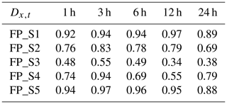
To identify the interaction between fluvial flooding and pluvial flooding, this study divides flood events into five stages, with key time points being the river water level exceeding the outfall elevation and riverbank overtopping. Stage 1 (FP_S1) means that the river water level is below the outfall elevation. Stage 2 (FP_S2) means that the river water level exceeds the elevation of the drainage outfall until the river overflows its bank. Stage 3 (FP_S3) is the riverbank overtopping stage. Stage 4 (FP_S4) means that the riverbank overtopping continues until the river water level drops below the outfall elevation. Stage 5 (FP_S5) means that the river water level recedes and does not exceed the outfall elevation again until the simulation ends.

The severity of fluvial flooding is analyzed through the percentage of fluvial flooding volume to the total flood volume (F_S3), as shown in Eqs. (16) to (17). In the storm flood model, the scenario where the drainage outfall is not connected to the river is set as the baseline scenario to simulate flooding. The change in flood volume relative to the baseline scenario (FP) is used to analyze the impact of interactions between the river and drainage outfall on flooding, as shown in Eq. (18). As fluvial flooding does not occur in the baseline scenario, only pluvial flooding is present. Therefore, for any duration, the difference between FP and F_S3 represents the percentage of inundation volume due to the jacking effect at the drainage outfall by the river.

$$\begin{array}{}\text{(16)}& F\mathit{\_}\mathrm{S}{\mathrm{3}}_t={\displaystyle \frac{V_{F\mathit{\_}\mathrm{S}{\mathrm{3}}_t}}{V_t}},\end{array}$$

$$\begin{array}{}\text{(17)}& V_t=\mathrm{FP}\mathit{\_}\mathrm{S}{\mathrm{1}}_t+\mathrm{FP}\mathit{\_}\mathrm{S}{\mathrm{2}}_t+\mathrm{FP}\mathit{\_}\mathrm{S}{\mathrm{3}}_t+\mathrm{FP}\mathit{\_}\mathrm{S}{\mathrm{4}}_t+\mathrm{FP}\mathit{\_}\mathrm{S}{\mathrm{5}}_t,\end{array}$$

$$\begin{array}{}\text{(18)}& {\mathrm{FP}}_t={\displaystyle \frac{\left({\mathrm{PF}}_t-V_t\right)}{V_t}},\end{array}$$

where V_t is the compound flood volume; $V_{\mathrm{F}\mathrm{\_}\mathrm{S}{\mathrm{3}}_t}$ represents the fluvial flooding volume with a duration of t in FP_S3; FP_S1_t, FP_S2_t, FP_S3_t, FP_S4_t, and FP_S5_t, respectively, represent the flooding volume with a duration of t in each stage; and PF_t represents the flooding volume which lasts for t hours and where the outfalls are not connected with the river.

To further explore the relative contributions of rainfall and tide levels to each stage, the method in Sect. 3.4 is used to calculate the impact index of rainfall and tide levels at each stage of flooding. For smaller return periods, the river water level may not exceed the elevation of the drainage outfall, and no fluvial flooding occurs. In this case, the flood volumes FW_S1, FW_S2, FW_S3, FW_S4, and FW_S5 are $V_t/\mathrm{2}$, 0, 0, 0, and $V_t/\mathrm{2}$, respectively. If the river water level exceeds the elevation of the drainage outfall but no fluvial flooding occurs, the flood volumes FW_S1, FW_S2, FW_S3, FW_S4, and FW_S5 are FP_S1_t, (V_t−FP_S1_t−FP_S5_t)/2, 0, (V_t−FP_S1_t−FP_S5_t)/2, and FP_S5_t, respectively.

3.6 Spatial analysis of compound flooding

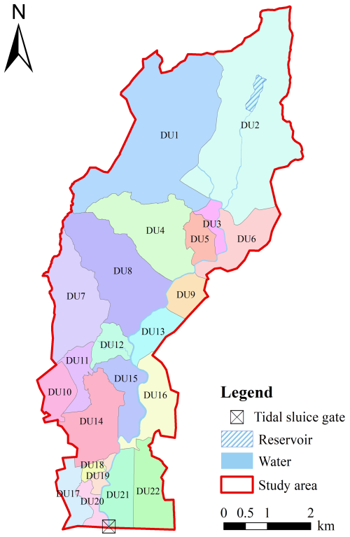
To analyze the spatial distribution differences of the driving factors of compound flooding, this study examines natural and social factors triggering flooding at the drainage unit level. The study area comprises 22 drainage units (Fig. 3), with specific division steps detailed in Sect. S2 in the Supplement. By analyzing the inundation area of each drainage unit, the spread of flooding in different units is assessed, and areas potentially affected by compound flooding are identified.

Figure 3 Diagram of drainage units (DUs) in study area.

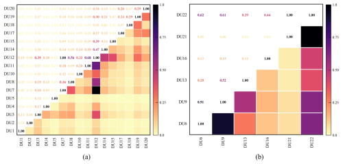
Flooding in each drainage unit is influenced through various pathways, including pipes, rivers, and surface routes. Identifying the key drainage units most closely linked with others is crucial for effectively formulating flood management strategies. This study draws on the principles of the urban gravity model to quantify the interaction force between drainage units (Zhao et al., 2021). Spatial interaction force represents the connection strength between drainage units. A higher interaction value indicates a stronger spatial influence of the drainage unit, warranting more attention in flood management. The calculation formula is as follows:

$$\begin{array}{}\text{(19)}& T_{ij}=k{\displaystyle \frac{Q_i^{\mathit{\alpha }}{Q}_j^{\mathit{\beta }}}{d_{ij}^{\mathrm{2}}}},\end{array}$$

where T_ij represents the spatial interaction value between drainage unit i and drainage unit j; d_ij represents a comprehensive distance index from the center of drainage unit i to the center of drainage unit j; Q_i and Q_j represent the flood control capacity of drainage unit i and drainage unit j, respectively; and coefficients k, α, and β are set to 1.

The length of the drainage network represents the drainage capacity, while the flooding volume indicates the degree of drainage obstruction. In this study, the percentage of the drainage network length of the drainage unit and flooding volume are combined to serve as the quality indicator in the urban gravity model. The formula for the calculation is as follows:

$$\begin{array}{}\text{(20)}& Q_i={\displaystyle \frac{l_i}{l{V}_i}},\end{array}$$

where l_i represents the length of the drainage network for drainage unit i, l represents the total length of the drainage network in the study area, and V_i represents the flooding volume of drainage unit i.

4 Results

4.1 Joint distribution and combination design of rainfall and tide level

By statistically analyzing daily rainfall and corresponding maximum tide level data, the Pearson correlation coefficient, Kendall correlation coefficient, and Spearman correlation coefficient were calculated as 0.89, 0.83, and 0.88, respectively. These results indicate a significant positive correlation between rainfall and tide levels, suitable for establishing a joint distribution function for analysis.

The study first established the marginal distributions of rainfall and tide levels, with the fitting results shown in Table S1. Based on the optimal marginal distribution functions, the two-dimensional copula models were established, with the fitting effectiveness shown in Table S2. The fitting effectiveness of each distribution function is satisfactory (Fig. 4), indicating their suitability for designing combinations of rainfall and tide levels. From the two-dimensional joint probability distribution of rainfall and tide levels for the 24 h duration (Fig. 4d), it is observed that the joint probability of less than 0.5 occupies a large area, indicating that the joint probability of rainfall and tide level exhibits a sharp peak and heavy tail characteristic. This means that a large amount of data are concentrated in a certain interval, while other data are widely distributed across various intervals, covering a broad range.

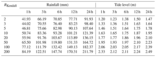
To compare results for different types of bivariate return periods, the study calculated the bivariate return periods after combining rainfall and tide levels with the same return period (Table S3). The results show that for univariate return periods of rainfall and tide levels, the “Or” return period is less than the “Kendall” return period, which is in turn less than the “And” return period. This indicates that the Kendall return period avoids overly large or small estimates of risk areas and can reasonably describe the return periods of combined variable events. Therefore, based on the Kendall return period, the design values of rainfall and tide levels for different durations and return periods were calculated, as shown in Table 1. The rainfall and tide level processes were implemented in accordance with Sect. 3.2.3 for flood simulation (Fig. 5).

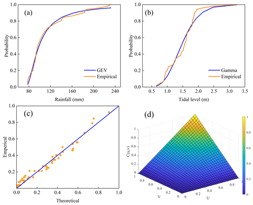
Figure 4 The joint distribution results of the 24 h duration. (a) The optimal marginal distribution of rainfall; (b) the optimal marginal distribution of tide level; (c) the optimal copula distribution function and empirical distribution function; (d) the joint probability distribution.

Table 1 Rainfall–tide-level design value.

Figure 5 Design process of rainfall and tide level with the 200-year RP: the sequence of durations from (a) to (e) are 1, 3, 6, 12, and 24 h durations.

4.2 Relative contributions of rainfall and tide levels to compound flooding

The relative contributions of rainfall and tide levels to compound flooding are crucial factors to consider in understanding the dynamics of flooding events. While rainfall can lead to increased surface water runoff and overwhelm drainage systems, high tide levels can exacerbate flooding by reducing the capacity of rivers and streams to discharge water into the ocean. Therefore, a comprehensive analysis of both rainfall patterns and tide levels is essential for effective flood risk management and mitigation strategies.

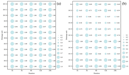
The impact indices of rainfall on flooding are shown in Fig. 6. It can be seen that the impact indices for DU1 to DU14 and DU17 are close to 1, indicating that the contribution of tide levels to flooding in these drainage units is essentially zero. The impact indices for DU15 to DU16 and DU18 to DU22 are around 0.5, suggesting that flooding in these drainage units results from the combined effects of rainfall and tide levels. The impact indices for DU15, DU16, and DU18 are higher than those for DU19 to DU22, indicating that as the distance from the drainage units to the Shahe River and Pearl River increases, the relative contribution of tide levels to compound flooding decreases. Additionally, DU21 has the smallest impact index, indicating a significant influence from tide levels. This is due to the presence of drainage outfalls discharging into the Pearl River within the drainage unit, posing a risk of tide backflow. DU21 is also adjacent to the river, experiencing indirect effects from tide levels.

Comparing the impact indices for different durations reveals that, overall, the impact indices for long durations are lower than those for short durations, indicating a trend of sustained increase in the contribution of tide levels to compound flooding as the simulation time extends. In short-duration scenarios (1 and 3 h durations), except for DU21, which is directly affected by tide levels, other drainage units have higher impact indices for the 3 h duration than for the 1 h duration, indicating that the contribution of rainfall to compound flooding increases with duration. This is because the influence time of tide levels for the 1 and 3 h durations is relatively short, and the total rainfall for the 3 h duration is larger, leading to more rain water entering the drainage system or river, exacerbating flood hazards. In long-duration scenarios, for DU19 to DU22, the impact index is highest for the 12 h duration, indicating significant rainfall effects at this duration. This is because these drainage units are close to the Pearl River and are greatly influenced by tide levels. Compared to the 12 h duration, the influence time of tide levels is shorter for the 24 h duration; however, compared to 6 h duration, the tide level difference is smaller although the total rainfall is larger. For DU15 and DU18, the impact index is lowest for the 12 h duration, possibly because these drainage units are far from the Pearl River and mainly influenced by rainfall. In comparison, the 12 h rainfall intensity is less concentrated than the 6 h duration, and the total rainfall is less than the 24 h duration, thus having a relatively smaller impact on flooding. Across the study area, the impact index is greater than 0.5, with the minimum at the 24 h duration being 0.69. This indicates that coastal compound flooding is primarily driven by the combined effects of rainfall and tide levels, with the contribution of tide levels being most significant at the 24 h duration.

4.3 Analysis of the interaction between fluvial flooding and pluvial flooding

When the river water level exceeds the elevation of the drainage outfall, it exerts the jacking effect on the outfall. The jacking time was summarized, as shown in Fig. 7. Generally, the average jacking duration increases with longer durations and higher return periods. The distance between the upper and lower edges of the box plot and the mean is considerable, and the box is relatively high, indicating significant variability in jacking duration among different drainage outfalls. For example, outfall O1 (Fig. S2) experiences jacking only at the 2 h duration and 200-year return period, with a jacking duration of 0.2 h. In contrast, outfall O2 (Fig. S2) is affected by river jacking almost throughout the simulation, with a maximum jacking duration of 23.92 h.

Figure 6 Comparison of the impact degree indices.

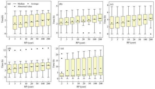
Figure 7 The average jacking time of the drainage outfalls: the sequence of durations from (a) to (e) is 1, 3, 6, 12, and 24 h.

From 1 h to 24 h durations, the maximum values of F_S3 are 15.35 %, 26.51 %, 23.68 %, 12.07 %, and 19.14 %, respectively, indicating that fluvial flooding accounts for about 1/5 of compound flooding. The differences between the maximum values of FP and the corresponding F_S3 are 8.25 %, 12.65 %, 11.60 %, 19.08 %, and 16.56 %, respectively, indicating that approximately 10 % of compound flooding is caused by the jacking effect of the river on the drainage outfall. This demonstrates that rivers not only directly influence coastal urban flood risk by causing fluvial flooding but also exacerbate pluvial flooding through the jacking effect, further increasing the severity of compound flooding in coastal cities.

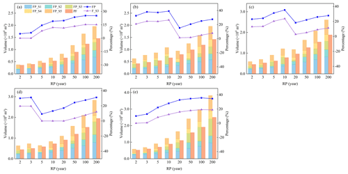
Figure 8 Comparison of flooding volume with or without river; the sequence of durations from (a) to (e) is 1, 3, 6, 12, and 24 h.

The impact indices of rainfall and tide levels at each stage of flooding are shown in Table 2. For any duration, the impact index decreases and then increases from FP_S1 to FP_S5, with the lowest impact index at the FP_S3 stage. This indicates that during FP_S2 to FP_S4, the relative contribution of tide levels to compound flooding is significant, especially at FP_S3. Except for the FP_S3 stage, the impact indices for other stages are greater than 0.5, indicating that compound flooding during these stages is predominantly influenced by rainfall, while the contribution of tide levels is more pronounced at the FP_S3 stage.

Table 2 Impact degree indices at different stages.

4.4 Spatial analysis of compound flooding and its driving factors

From the results of maximum inundation depth in Fig. 9, it is evident that flood risk significantly increases with longer rainfall durations and higher return periods. Specifically, the flood extent expands in DU1, DU2, DU4, DU5, DU10, and DU13, with flood risk levels rising from moderate (0.5–1 m) to severe (more than 1 m). Furthermore, there is severe waterlogging in DU8 and DU14 to DU22, and moderate waterlogging in DU4 also increases. It is important to note that the most severe flood risk area is located midstream, particularly under a 1 h duration and a 2-year return period. However, under a 24 h duration and a 200-year return period, the most severe area shifts downstream. Combined with the analysis in Sect. 4.2, this is because the influence of tide levels on flooding gradually strengthens with increasing rainfall duration, particularly affecting downstream areas. This indicates that tide levels drive the shift of compound flood risk towards downstream areas in coastal cities.

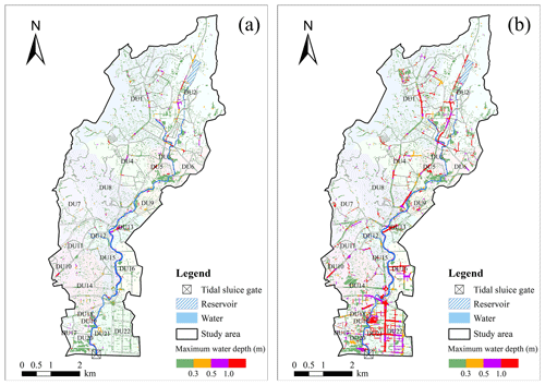
Figure 9 Inundation extent and water depth under 24 h scenarios: (a) 2-year return period; (b) 200-year return period.

The interaction strength between different drainage units is shown in Fig. 10. On the right bank of the river (Fig. 10a), DU12 exhibits significant interaction with other units, indicating that, as an intermediate node, it has notable interactions with upstream and downstream water flows. On the left bank of the river (Fig. 10b), DU22 has a strong spatial interaction with other drainage units, even with the distant DU6. This highlights that DU22 and DU12 play crucial roles in the entire drainage network and should receive focused attention in flood management.

Combining the analyses in Sect. 4.2 and 4.3, this study identifies the driving factors of compound flooding from both natural and social perspectives. Pluvial flooding occurs in DU1 to DU22 due to rainfall and drainage networks. Tide levels affect DU14 to DU16 and DU18 to DU22. The drainage outfalls in DU6, DU8, DU9, DU12 to DU16, DU19, and DU21 are subject to the jacking effect from rivers. Additionally, fluvial flooding occurs in DU15, DU16, DU19, and DU21. Based on these results, the driving factors of compound flooding can be categorized into five classes. Class I involves the combined effect of rainfall and the drainage network. Class II comprises rainfall, the drainage network, and drainage outfalls. Class III includes rainfall, tide levels, and the drainage network. Class IV consists of rainfall, tide levels, the drainage network, and drainage outfalls. Class V extends Class IV by adding riverbank defenses. Classes I–IV represent the causes of pluvial flooding, while Class V represents the causes of general flooding. The classification of drainage units into these causal categories is presented in Fig. 11.

5 Discussion

5.1 Driving factors of compound flooding in coastal cities

Compound flooding in coastal cities is influenced by complex factors. Rainfall is the primary driving factor of compound flooding, significantly impacting pluvial flooding (Fig. 6 and Table 2). Previous studies have focused on analyzing pluvial flooding induced by heavy rainfall (Zhang et al., 2017, 2021; Zou et al., 2022). However, in coastal cities, tide levels are also important driving factors. Tide levels obstruct river drainage, causing a jacking effect on drainage outfalls, with the maximum jacking duration reaching up to 23.92 h (Fig. 7). When drainage outfalls are subjected to the jacking effect, drainage becomes inefficient, leading to an increase in flood volume by approximately 10 % (Fig. 8). Under the influence of tide levels, flooding in coastal cities not only manifests as pluvial flooding but also includes fluvial flooding. The proportion of fluvial flood volume to total flood volume reaches 26.51 % (Fig. 8). In summary, compound flooding in coastal cities results from the complex interplay of rainfall, tide levels, drainage networks, drainage outfalls, and rivers.

However, when examining flooding issues at a microscale, there are more specific details and particular situations that need attention. For instance, clogged or debris-laden stormwater grates can affect the normal discharge of rainwater, potentially leading to localized flooding issues. Aging or damaged drainage pipes may risk leakage or collapse, hindering the flow of water and causing flooding (Mohandes et al., 2022).

5.2 Impact of rainfall and tide level on flooding

In scenarios where drainage outfalls allow for free flow, the severity of flooding is primarily governed by rainfall. When the rainfall pattern is the same, a larger total rainfall results in more severe flooding (PF in Fig. 8). However, under the same return period, there are instances where the flood volume for longer durations is less than for shorter durations. For example, in Fig. 8, for return periods of 100 and 200 years, the pluvial flooding volume for the 1 h duration exceeds that for the 3 h duration, and for return periods of less than 100 years, the pluvial flooding volume for the 6 h duration exceeds that for the 12 h duration. This indicates that besides total rainfall, the rainfall process significantly affects flooding. The total rainfall for the 1 h duration is less than for the 3 h duration, but the average rainfall intensity is higher (Fig. S4a). As the return period increases, the difference in total rainfall between 1 and 3 h durations decreases. In contrast, the difference in average rainfall intensity increases, leading to the average rainfall intensity having a greater impact on flooding than total rainfall. A similar comparison applies to 6 h duration and 12 h duration (Fig. S4b). Thus, under rainfall-only conditions, flood intensity is not determined solely by total rainfall or rainfall intensity.

Considering the effect of tide levels, it is observed that flood volumes for shorter return periods exceed those for longer return periods under the same duration (Fig. S5). For instance, at the 3 h duration, return periods of 10 and 20 years show a significant difference. This difference is mainly evident in stage FP_S3 (Fig. 8). Combining the tidal sluice gate (hereinafter referred to as “gate”) opening times with flood processes (Table S4 and Fig. S6), it is found that this is because the gate opening time for a 10-year return period is later than for a 20-year return period. With more rainfall for the 20-year return period, river water levels rise quickly due to increased rainfall, leading to gate opening conditions occurring earlier. In contrast, the 10-year return period experiences less rainfall and fewer instances of pipe overflow (Fig. S6a); as the river water level rises slowly, the gate opening is delayed, ultimately leading to severe overflow as shown in Fig. S6b. Similarly, for durations of 6 and 12 h (Table S4 and Fig. S6), the gate opening times are earlier for return periods of 20 and 5 years, respectively, resulting in smaller flood volumes than for return periods of 10 and 3 years. This also explains the abrupt changes in FP and F_S3 in Fig. 8. The above analysis indicates that the combined effect of rainfall and tide levels does not increase proportionally with the return period.

Figure 10 Spatial interaction between different drainage units.

Figure 11 Diagram of flood causes by drainage units.

The effect of tide levels also changes the comparison results of flood volumes under the different durations in rainfall-only conditions. For instance, under return periods of 2 and 3 years, the flood volumes for 3 and 12 h durations exceed those for the 6 h duration, and the flood volume for the 12 h duration exceeds that for the 24 h duration. Specifically, during the 3 h rainfall process, the gate does not open, causing drainage difficulties and severe overflow. In the 6 h scenario, the gate opens for drainage, alleviating river pressure (Table S4 and Fig. S6). For the 12 h duration, although the average rainfall intensity is less than for the 6 h duration, the gate opening is delayed, and the large rainfall volume leads to severe river overflow, exceeding the flood volume for the 6 h duration. In the 24 h scenario, due to timely gate opening after the peak rainfall, the river drainage capacity is strong, with almost no river overflow. It is evident that the operation of the gate directly affects the drainage capacity of the river, resulting in significant differences in flood volume. The gate's status is influenced by multiple factors, including total rainfall, peak tide levels, and the time interval between peak rainfall and peak tide level. A larger total rainfall, higher rainfall intensity, or shorter time interval do not necessarily hinder the gate's operation, nor do they always result in larger flood volumes. Therefore, under the influence of tidal levels, the factors affecting the severity of flooding become more complex.

5.3 Implications for flood management in coastal cities

The study results highlight the complexity of driving factors for compound flooding. Therefore, appropriate management measures should be adopted for different flood causes. As shown in Fig. 11, drainage units classified as Classes III to V are impacted by tide levels, necessitating the use of high-capacity pumping facilities to reduce flood risk. For units classified as Classes II, IV, and V, there are concerns regarding unreasonable drainage outfall elevations, with Class V also experiencing river overtopping. It is suggested to research river and outfall design standards that are more suitable for current and future climate conditions, while exploring ecological engineering methods to enhance the performance of rivers and drainage outfalls. For drainage outfalls directly affected by tidal jacking, planning external barriers to prevent tidal backflow is necessary. Additionally, the stormwater retention capacity within the city should be improved, implementing a combined retention and drainage strategy to minimize peak flood discharge, thereby alleviating the pressure from interactions among different types of flooding. This is beneficial for addressing various flood causes. Furthermore, drainage units with significant spatial interaction should receive focused attention to enhance the flood control capacity of the entire drainage system.

5.4 Limitations

The data length not only affects copula modeling but also has an adverse effect on the marginal distributions (Tong et al., 2015). Intuitively, longer-term data provide better modeling results. This study uses 16 years of data to estimate a 200-year return period event, introducing significant uncertainty in modeling dependence structures and tail distributions. With further data accumulation, future studies are expected to utilize longer-term data to improve analysis precision and accuracy. Although this study quantifies the relative contributions of total rainfall and peak tide level to compound flooding under different return periods and durations, it does not consider the impact of rainfall's temporal distribution or the time interval between peak rainfall and peak tide level. Future research should design multivariate joint distributions that comprehensively consider rainfall temporal characteristics and time intervals to more fully reveal the influence of natural factors on compound flooding. Additionally, the analysis of spatial interaction forces among drainage units is significant for flood management, but the current indicators that were used have certain limitations. We plan to adopt more comprehensive indicators in the future to enhance the depth and breadth of spatial analysis, better serving the formulation of flood management strategies.

6 Conclusions

Exploring the driving factors of compound flooding in coastal cities is of significant importance for scientific research and flood management. This study employs a hydrodynamic model and multivariate statistical methods to quantify the relative contributions of rainfall and tide levels to compound flooding in coastal cities and analyzes the interactions among different types of flooding. The driving factors of compound flooding were ultimately identified. The main conclusions are as follows:

1. Compound flooding in coastal cities results from the combined effects of multiple factors, including rainfall, tide levels, drainage pipes, drainage outfalls, and rivers. Rainfall generates runoff that enters the drainage pipes, leading to pluvial flooding when the drainage capacity is insufficient. The pipes discharge water into rivers through drainage outfalls, but tide levels obstruct river drainage, causing fluvial flooding in areas with lower riverbank elevations.

2. The combination of the copula function and Kendall return period method is effective for designing hydrological variable combinations. The study shows that the optimal joint distribution function for 24 h rainfall and tide levels is the Frank copula, with an R² of 0.97 compared to the empirical distribution function. The Kendall return period lies between the “Or” return period and the “And” return period, avoiding excessively large or small combination design values.

3. Compound flooding in coastal cities is influenced by the combined effects of rainfall and tide levels, with rainfall having a relatively greater contribution. From 1 to 24 h durations, the impact index of rainfall and tide levels on compound flooding changes from 0.83 to 0.69 and from 0.17 to 0.31, respectively. This indicates that rainfall predominantly contributes to compound flooding, while the effect of tide levels is most significant at the 24 h duration.

4. Rivers worsen compound flooding in coastal cities by elevating drainage outfalls and causing fluvial flooding. Due to tide levels, rivers elevate drainage outfalls for a duration of up to 23.92 h, resulting in a maximum increase of 19.08 % in pluvial flooding volume. More critically, fluvial flooding occurs, with its volume accounting for a maximum of 26.51 % of the total flood volume.