Learning landscape features from streamflow with autoencoders

Recent successes with machine learning (ML) models in catchment hydrology have highlighted their ability to extract crucial information from catchment properties pertinent to the rainfall–runoff relationship. In this study, we aim to identify a minimal set of catchment signatures in streamflow that, when combined with meteorological drivers, enable an accurate reconstruction of the entire streamflow time series. To achieve this, we utilize an explicit noise-conditional autoencoder (ENCA), which, assuming an optimal architecture, separates the influences of meteorological drivers and catchment properties on streamflow. The ENCA architecture feeds meteorological forcing and climate attributes into the decoder in order to incentivize the encoder to only learn features that are related to landscape properties minimally related to climate. By isolating the effect of meteorology, these hydrological features can thus be interpreted as landscape fingerprints. The optimal number of features is found by means of an intrinsic dimension estimator. We train our model on the hydro-meteorological time series data of 568 catchments of the continental United States from the Catchment Attributes and Meteorology for Large-sample Studies (CAMELS) dataset. We compare the reconstruction accuracy with models that take as input a subset of static catchment attributes (both climate and landscape attributes) along with meteorological forcing variables. Our results suggest that available landscape attributes can be summarized by only two relevant learnt features (or signatures), while at least a third one is needed for about a dozen difficult-to-predict catchments in the central United States, which is mainly characterized by a high aridity index. The principal components of the learnt features strongly correlate with the baseflow index and aridity indicators, which is consistent with the idea that these indicators capture the variability of catchment hydrological responses. The correlation analysis further indicates that soil-related and vegetation attributes are of importance.

1 Introduction

Hydrological signatures encompass descriptive statistics derived from meteorological and streamflow time series. They serve various purposes in hydrology, such as hydrological model calibration or evaluation (Fenicia et al., 2018; Kiraz et al., 2023), process identification (McMillan, 2020a), and ecological characterization (Olden and Poff, 2003). Along with catchment attributes (distinguished here in landscape and climate attributes), they are also used for catchment classification and regionalization studies (Wagener et al., 2007).

Streamflow signatures, i.e. hydrological signatures based solely on streamflow, have significant importance as they relate to the variable one aims to predict and understand (Gnann et al., 2021). Hydrologists have developed diverse signatures reflecting different aspects of streamflow dynamics. Examples include those linked to the flow duration curve (e.g. the slopes of various segments), the baseflow index, or the flashiness index. Numerous other such signatures exist. For instance, Olden and Poff (2003) compiled a list of 171 indices from prior work, reflecting aspects associated with the magnitude, frequency, duration, timing, and rate of change of flow events. As streamflow depends on meteorological forcing and landscape attributes, streamflow signatures generally contain information from both sources. In particular, for predictions in ungauged basins, it is vital to be able to disentangle them.

One way of doing so is through hydrological models, which condense catchment attributes into model parameters (Wagener et al., 2003). Previous research indicates that observed hydrographs can be represented by a handful of model parameters (Jakeman and Hornberger, 1993). For instance, the GR4J (Génie Rural à 4 paramèters Journalier) model (Perrin et al., 2003), resulting from a continuous refinement process aimed at balancing model complexity and performance, has only four parameters. However, these analyses are based on pre-defined model assumptions.

Model parameters can, in principle, be directly estimated from streamflow signatures. The approximate Bayesian computation (ABC) technique (Albert et al., 2015) was recently used to infer model parameters from streamflow signatures – which in this context are called summary statistics – bypassing the need to directly compare the complete time series (Fenicia et al., 2018). If these summary statistics contain all the information necessary to estimate model parameters, they are termed sufficient. Sufficiency is therefore not an inherent property of the summary statistics but depends on the specific hydrological model and on the parameters that need to be inferred. For ABC to converge efficiently, we also want the summary statistics to be minimal. That is, while they should ideally encode all the parameter-related information available in the streamflow, they should encode no other information, whether from the forcing or the noise that is used for the simulations (Albert et al., 2022). Such minimally sufficient summary statistics could thus be considered the relevant fingerprints of landscape features in the streamflow. Of course, this only holds true if the model is capable of encoding all the information in such features that is relevant to the input–output relationship. However, recent studies show that purely data-driven models outperform process-based models in prediction accuracy (Kratzert et al., 2019; Mohammadi, 2021), because they suggest information on catchment attributes previously not utilized for streamflow prediction.

Our goal is to employ machine learning (ML) techniques to identify a minimal set of streamflow features enabling accurate streamflow predictions when combined with meteorological forcing. Thus, our aim is to eliminate all forcing-related information from the streamflow, distilling features solely from the catchments themselves. We approach this objective from a purely data-driven perspective.

To identify minimal sets of streamflow features, we employ an explicit noise-conditional autoencoder (ENCA) (Albert et al., 2022), where the bare noise utilized by the stochastic model simulator is fed into the decoder together with the learnt summary statistics. In this way, the encoder is encouraged to encode only those features containing information on the model parameters while disregarding the noise. Albert et al. (2022) applied ENCA to infer parameters of simple one-dimensional stochastic maps, showing that the learnt features allow for an excellent approximation of the true posterior. In our case, instead of noise, we input meteorological forcing into the decoder. By also feeding climate attributes into the decoder, we encourage the encoder to exclusively encode landscape-related information within the streamflow. Moreover, since we make use of unidirectional long short-term memory (LSTM) networks (see Appendix C), conditioning ENCA on climate attributes could also help the decoder to obtain future information on the climate that it would not normally be able to retrieve.

In order to reduce the computational costs and learn a minimal set of catchment features, the dimension of the latent space is chosen according to the estimation of its intrinsic dimension (ID) (Facco et al., 2017; Allegra et al., 2020; Denti et al., 2022). In particular, we employ the ID estimator GRIDE (Generalized ratios intrinsic dimension estimator) (Denti et al., 2022), which is robust to noise. Learnt features will then be compared with known catchment attributes (from both the landscape and climate) and hydrological signatures to provide a hydrological interpretation and guide knowledge domain experts towards the pertinent information necessary for streamflow prediction.

We apply our approach to the CAMELS (Catchment Attributes and Meteorology for Large-sample Studies) dataset (Newman et al., 2015), covering several hundred catchments over the contiguous United States (CONUS). LSTM networks have emerged as state-of-the-art models for streamflow data-driven predictions. In the study by Kratzert et al. (2019), LSTMs validated on unseen catchments, enriched with static landscape and climate attributes from Addor et al. (2017), outperformed conceptual models. The first investigations of the mechanistic interpretation of LSTM states, e.g. linking hidden states to the dynamics of soil moisture, demonstrated the potential to elicit physics from data-driven models (Lees et al., 2022). Here, by linking learnt features to known catchment attributes, we explore a further aspect of this broader field of explainable AI or interpretable ML (Molnar, 2024; Molnar et al., 2020).

Our specific objectives are (i) to find the minimal number of dominant streamflow features stemming from the landscape and (ii) to relate them to known landscape and climate attributes as well as established hydrological signatures. This will allow us not only to determine how many features are required for streamflow prediction but also to answer the question of whether there is missing information on known catchment attributes.

A similar attempt to learn signatures was recently made by Botterill and McMillan (2023). In pursuit of an interpretable latent space on the continental scale, they employed a convolutional encoder to compress high-dimensional information derived from meteorological forcing and streamflow data. This approach aimed to learn hydrological signatures (McMillan, 2020b) within the US-CAMELS dataset. It differs from ours in three aspects: (i) they used a traditional conceptual model as a decoder, whereas we use an LSTM architecture which has been shown to be superior to conceptual models when provided with catchment properties; (ii) they fed both streamflow and meteorological forcings into the encoder, whereas we feed only streamflow data in an attempt to separate landscape and forcing information; and (iii) they did not attempt to find a minimal number of signatures that was sufficient for streamflow prediction, whereas this is a primary objective of our work.

It is important to note that our main objective is not to beat state-of-the-art models regarding their predictive performance (Kratzert et al., 2021; Klotz et al., 2022). Our goal is rather to investigate the information content of streamflow. However, we believe that our research will provide valuable insights into the most critical features of streamflow prediction.

2 Models and methods

2.1 Data

We employ the Catchment Attributes and Meteorology for Large-sample Studies (CAMELS) (Newman et al., 2015), which consists of 671 catchments in the CONUS, ranging in size from 4 to 25⋅10³ km². For this study, we select those 568 catchments out of 671 whose data span continuously on a daily basis the time period from 1 October 1980 to 30 September 2010, corresponding to 30 hydrological years. The first 15 years are used for training and the last 15 for testing. Along with the streamflow time series and the meteorological forcing variables, US-CAMELS also provides information about static catchment attributes (Addor et al., 2017), encompassing both landscape (vegetation, soil, topography, and geology) and climate. Streamflow data are retrieved from US Geological Survey gauges, while the meteorological forcing comes from the extended North America Land Data Assimilation System (NLDAS) (Kratzert, 2019) and includes maximum and minimum daily temperatures, solar radiation, vapour pressure, and precipitation.

2.2 Explicit noise-conditional autoencoder (ENCA)

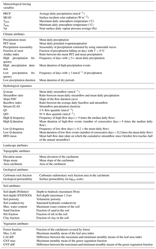
Following Albert et al. (2022), we feed the streamflow into a convolutional encoder. ENCA has been designed to distil sufficient summary statistics which contain minimal noise information from the output of stochastic models. Here (Fig. 1 – for the detailed architectures, the reader is referred to Appendix C), the noise is substituted by all the variables we are not interested in, i.e. the meteorological forcing. The convolutional encoder is thus followed by an LSTM decoder that takes as input 15 hydrological years of meteorological forcing, i.e. 5478 time points, and nine climate attributes (reported in Table 1). The LSTM capacity is limited by the dimension of the input layer. In order to enlarge the available capacity and capture more complex patterns from the meteorological forcing, the meteorological time series are first fed into a single linear layer with 1350 output units. The output of this linear layer is then concatenated with the output of the encoder and fed into the LSTM decoder. In this way, the decoder sees tensors of size (BS, $\mathrm{5478},\mathrm{1350}+N$), where BS is the batch size (the batches are selected across different catchments) and N is the latent space dimension. We opted for such an architecture in order to extract as much static information related to the streamflow as possible.

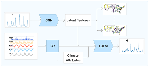
Figure 1 The explicit noise-conditional autoencoder used in this study. For the hyper-parameters and the implementation details, the reader is referred to Appendix C. The neural network architectures employed are a convolutional neural network (CNN), a fully connected (FC) layer, and a LSTM. The observed and simulated streamflows are denoted by Q and $\widehat{\mathrm{Q}}$, respectively. The meteorological forcing variables are denoted by PRCP (precipitation), SRAD (solar radiation), T_max (maximum temperature), T_min (minimum temperature), and Vp (vapour pressure).

We expect to be able to compress almost all streamflow information not already contained in the forcing into a low (N)-dimensional feature vector¹. Because they should be largely devoid of forcing information, we call these the relevant landscape features and explain in Sect. 2.4 how we fix their number. In principle, these features are hydrological signatures (since they are functions of the streamflow) that contain as little information as possible about the forcing and the climate. However, this can only be achieved if the decoder is capable of utilizing all the available information in the meteorological drivers, which is never fully realized in practice. Also, the sufficiency of the learnt features is not guaranteed a priori and depends on the encoder architecture that is employed, which here is a convolutional network.

Comparing relevant landscape features with known static catchment attributes in terms of their capacity for streamflow reconstruction will allow us to find out whether static catchment attributes lack information that is crucial for streamflow prediction. For this comparison, we use an LSTM model augmented with catchment attributes (Addor et al., 2017) in the input, stemming from both the landscape and the climate. This is the Catchment Attributes Augmented Model (CAAM). This model differs from Fig. 1 solely by the fact that the latent features are substituted with known landscape attributes. Following Kratzert et al. (2019), CAAM is fed with 27 catchment attributes (reported in Table 1), which are representative of climate, topography, geology, soil, and vegetation.

In order to mitigate numerical instability, it is crucial to standardize the catchment attributes or latent features before feeding the LSTM. In CAAM, we standardize the catchment attributes with the mean and standard deviation computed over all the considered catchments. This is not possible for ENCA, since the mean and standard deviation of the latent features are not known a priori. Therefore, we standardize the latent features by means of a batch normalization layer. In this way, we ensure that the magnitude of the LSTM input is comparable between CAAM and ENCA.

2.3 Training and testing

We use the first 15 years of data for training and the last 15 years for testing. Training is performed by maximizing the Nash–Sutcliffe efficiency (NSE) (Nash and Sutcliffe, 1970), which is defined as

$$\begin{array}{}\text{(1)}& \mathrm{NSE}=\mathrm{1}-{\displaystyle \frac{{\sum }_{t=\mathrm{1}}^{\mathrm{T}}(q_{\mathrm{sim},t}-q_{\mathrm{obs},t}{)}^{\mathrm{2}}}{{\sum }_{t=\mathrm{1}}^{\mathrm{T}}(q_{\mathrm{obs},t}-{\mathit{\mu }}_{\mathrm{obs}}{)}^{\mathrm{2}}}},\end{array}$$

where q_obs,t and q_sim,t are, respectively, the observed and predicted streamflows (mm d⁻¹) at day t and μ_obs is the average of the observed streamflow. We notice that maximizing the NSE is equivalent to minimizing the mean square error (MSE) between the data and the prediction. Each model is trained with the Adam optimizer (Kingma, 2014), with a learning rate equal to 10⁻⁵ for 10 000 epochs. The batch size is set to 64, and the first 270 d of the predicted streamflow are excluded when computing the loss.

We also report the three components into which NSE can be decomposed: see Eq. (4) in the main text of Gupta et al. (2009). These components are the linear correlation coefficient (R), the bias normalized by the observed streamflow standard deviation (BIAS), and the standard deviation ratio (SD). The linear correlation coefficient is related to the timing, whereas SD measures the streamflow variability and is defined as

$$\begin{array}{}\text{(2)}& \mathrm{SD}={\displaystyle \frac{{\mathit{\sigma }}_{\mathrm{sim}}}{{\mathit{\sigma }}_{\mathrm{obs}}}},\end{array}$$

where σ_sim and σ_obs are the standard deviations of the simulated and observed streamflows, respectively. Finally, BIAS is related to volume errors and is defined as

$$\begin{array}{}\text{(3)}& \mathrm{BIAS}={\displaystyle \frac{{\mathit{\mu }}_{\mathrm{sim}}-{\mathit{\mu }}_{\mathrm{obs}}}{{\mathit{\sigma }}_{\mathrm{obs}}}}.\end{array}$$

Each algorithm is affected by noise, due to the random initialization of the neural network parameters. To minimize this effect, we run each model with four random restarts, each one providing the streamflow prediction for the whole testing period. We compute the evaluation metrics on the predicted streamflow after averaging the streamflow over these four random restarts.

2.4 Intrinsic dimension estimation

The selection of the encoder's latent space dimension, specifically the number of relevant features, is informed by the ID estimator GRIDE (Denti et al., 2022). We utilize the GRIDE paths, which involve estimating the ID at several distance scales at which the data are analysed (for an in-depth discussion on the ID, see Appendix A). The ID intuitively measures the dimension of the manifold where the data reside, which may be lower than the dimension of the embedding space. Most ID estimators depend on calculating the distance scale between data points, and the estimated ID itself can vary with this distance scale. Figure 2, derived from Denti et al. (2022), shows points on a one-dimensional line with added noise embedded in a three-dimensional space. When the distance scale is too small, the data points appear to fill the space uniformly, making the manifold seem three-dimensional. However, as the distance scale increases and the noise is bypassed, the estimated ID decreases until the correct value of one is achieved.

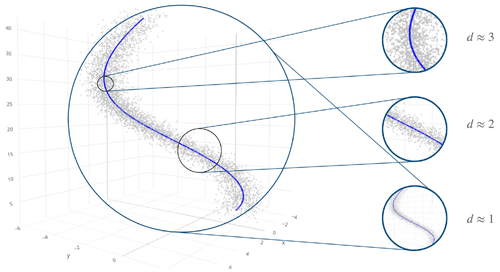
Figure 2 Unidimensional line with noise, embedded in three dimensions. The estimated intrinsic dimension depends on the distance scale.

To identify the dimension of the latent space of ENCA, we proceed with the following methodology. First, we train an ENCA-N with a relatively large number of latent features N. Since we fed 27 catchment attributes into the reference model (CAAM), we use a 27-dimensional latent space in order to have a fair comparison in terms of model capacity. We refer to this model as ENCA-27. The exact dimension of the latent space we start with does not matter much, as long as it is larger than the expected number of relevant landscape features. Then, we estimate the ID of the latent space and train another ENCA with a number of latent features equal to the estimated ID. In turn, we estimate its ID to check whether the dimension of the latent space can be reduced further. We thus use the ID as a guide to progressively diminish the dimension of the latent space of the autoencoder. However, in the end we train ENCA for several dimensions of the latent space and evaluate the information content of the learnt features in terms of their ability to reconstruct streamflows. In Fig. A1, we report GRIDE paths for the different models trained in this work.

3 Latent space interpretation

The relevant features are first projected using principal component analysis (PCA), since in general the autoencoder's latent representation is in arbitrary coordinates. In doing so, we ensure a fair comparison between the different random restarts, since we change the basis of each latent space by ordering the new coordinates according to the explained variance. Finally, in order to interpret the relevant landscape features, we report the absolute Spearman correlation (Zar, 2005) matrix among the learnt features, static catchment attributes, and hydrological signatures, which are reported in Table 1.

Table 1 The meteorological forcing variables, climate and landscape (topographic, geological, soil, and vegetation) attributes, and hydrological signatures compared in this study. Both climate and landscape attributes are fed into CAAM. ENCA models are conditioned on climate attributes too.

4 Results and discussion

4.1 The number of relevant landscape features

Figure 3 depicts the boxplot of the test NSE values for the considered models. We report and discuss the associated statistics, the boxplots of the NSE components (R, BIAS, and SD), and the correlations between them in Appendix B.

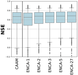
Figure 3 NSE values for the considered models in the test period. The boxes are delimited by the 25 % and 75 % quantiles, while the whiskers indicate the 5 % and 95 % quantiles. The CAAM performance is similar to that of ENCA-2.

In terms of NSE, we observe a performance improvement from ENCA-1 to ENCA-2 in the bulk of the distribution and a further minor improvement from ENCA-2 to ENCA-3. The NSE improvement between ENCA-3 and ENCA-5 is minor and is mainly related to outliers, while the ENCA-5 and ENCA-27 distributions are almost identical.

In general, Fig. 3 and the related statistics (Fig. B1) show that increasing the number of latent features improves the prediction accuracy of the considered metrics. Even though it is difficult to set a cut-off dimension, we can state that, (i) with more than five latent features, we no longer observe a performance improvement, meaning that five features form a sufficient set of summary statistics of the streamflow (which, however, can still depend on the chosen encoder architecture). (ii) Overall, the CAAM performance is most similar to that of ENCA-2. We therefore argue that known catchment attributes (selected in this study) account for two relevant landscape features that appear to be sufficient for most catchments, while at least a third one is needed to resolve specific catchments.

To study which catchments are most affected when using the latent features of the ENCA models in place of the known catchment attributes in CAAM, we report (Fig. 4) the NSE differences between CAAM and ENCA-2 (left panels) or ENCA-3 (right panels), respectively. While, for most of the catchments, switching from ENCA-2 to ENCA-3 does not result in a high performance gain, we see a clear improvement in about a dozen or so catchments mostly located in the central CONUS. This corroborates the hypothesis that the known catchment attributes account for two relevant landscape features, and the improvement due to the third one is related to only a few catchments that are particularly difficult to predict. It is interesting to count the number of catchments for which CAAM's NSE is negative (i.e. predictions that are worse than the average streamflow) but ENCA's NSE is positive. This number is 17 for ENCA-2 and 15 for ENCA-3. On the other hand, the number of catchments for which CAAM's NSE is positive but ENCA's NSE is negative decreases from eight (ENCA-2) to only two (ENCA-3).

Figure 4 Test NSE of ENCA-2 (a) and ENCA-3 (b) versus CAAM, colour-coded with the NSE difference per catchment clipped in [$-\mathrm{1},\mathrm{1}$]. Red means that ENCA performs better, and blue means that CAAM performs better.

In order to evaluate the impact of additional features, we compare the performances of ENCA models differing in their number of latent variables (Fig. 5). The results corroborate our earlier findings that two features are sufficient to cover most of the catchments, and additional features provide information on relatively few, difficult-to-predict catchments mostly located in the central CONUS and dominated by arid climate conditions. While the number of such catchments informed by the third feature is relatively high, additional features only have a minor effect. Indeed, adding a third feature turns seven catchments from a negative NSE to a positive NSE and leads to only marginal deterioration of three other catchments. Additional features have much less dramatic effects.

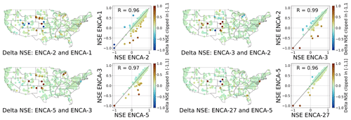
Figure 5 Test NSEs of ENCA models with different numbers of latent features, colour-coded according to the NSE difference per catchment clipped in [$-\mathrm{1},\mathrm{1}$]. The improvement from increasing the number of latent features is significant from ENCA-2 to ENCA-3 and marginal for more complex models. The improved catchments are mainly located in the central CONUS, which is dominated by arid climate conditions.

Note that the test NSEs obtained in this work are good but still far from state-of-the-art approaches to the same dataset. For comparison, the global model of Kratzert et al. (2019) (augmented with the same catchment attributes reported in Table 1) achieves a median NSE of 0.74, while in this work the best model achieves a median NSE of 0.68. Later approaches (with multiple input forcings) achieve an even higher performance of 0.82 (Kratzert et al., 2021). One might be tempted to attribute this to overfitting due to the very large number of parameters of our architecture (about 3 million). However, the test MSE loss curves (Fig. C1) do not support this hypothesis. Also, the very long sequences fed to LSTM might affect their performance, as they are known to suffer from vanishing or exploding gradients. While we use time series of length 5478, state-of-the-art approaches use lengths of 270 (Kratzert et al., 2019) and 365 (Kratzert et al., 2021).

4.2 Interpretation of the relevant feature principal components

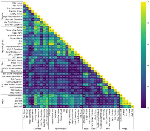
Figure 6 shows the absolute Spearman correlation matrix between the principal components of the three identified relevant features, the known streamflow signatures, and the catchment attributes across the different random restarts of the model. The relevant features share information with the catchment attributes and hydrological signatures. For instance, feature one carries information about basic hydrological attributes like the baseflow index and low-flow frequency. Moreover, feature one is (weakly) correlated with soil-related attributes like soil porosity and conductivity, sand, silt, and clay fraction. Feature two is correlated with climatic indicators like the aridity index, the mean precipitation, high and low precipitation frequency, and hydrological signatures like mean streamflow and the 95 % quantile of the flow duration curve. We point out that, even though the encoder is explicitly designed to learn non-climate landscape features, we can still observe a correlation between latent features and climate attributes. This correlation can be due to collinearities between landscape and climate attributes. In this case, the collinear attributes are those related to vegetation, like the fraction of forests and the maximum GVF (green vegetation fraction), which are obviously correlated with climate. For instance, from Fig. D1 we can observe that the aridity index is highly correlated with the mean precipitation (0.88) and the fraction of forest (0.74), while these last two attributes are fairly correlated with each other (0.67). Finally, feature three is mostly correlated with high- and low-flow duration and frequency, which are signatures relating to the extremes of streamflow. Interestingly, this principal component does not hold much information about landscape or climate attributes, indicating that it encodes catchment information that has not yet been considered or that is not related to any discernible catchment feature. Since the third feature mainly conveys information about certain dry and hard-to-predict catchments, the latter might very well be the case.

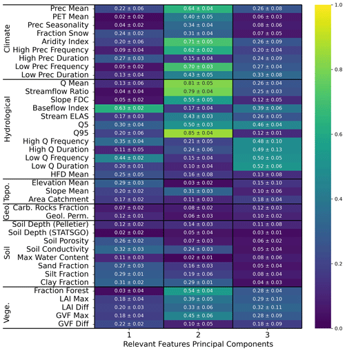
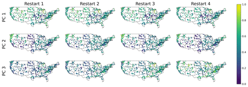
Figure 6 Average (plus or minus the standard deviation) of the absolute Spearman correlation of the relevant feature principal components of ENCA-3 with respect to the catchment attributes and hydrological signatures across the four different random model restarts. The colours refer to the average.

The discussed principal components, however, do not share the same amount of explained variance: feature one accounts for about 60 %, feature two for about 30 %, and feature three for about 10 %. In Appendix E we report the correlation matrices for the other ENCA models, where we can verify that the principal components carry the same information for streamflow prediction consistently across the different models.

The geospatial distribution of feature importance is shown in Fig. 7, where a non-trivial distribution of the features appears, highlighting that the different features have a different information content for the different regions: feature one dominates in the less arid to non-arid eastern CONUS, while feature two is mainly dominant in the western part. Feature three does not show such a clear spatial representation. Overall, the potential to delineate geospatial relations is another indicator that the encoder has learnt from the landscape signal in the data.

Figure 7 Principal components (PCs) of the relevant features of ENCA-3 in the CONUS. For a better comparison across different restarts, PCs are normalized in the interval [0,1] and their sign is adjusted such that the PCs of the first catchment in the dataset are always positive.

5 Conclusions and outlook

We employed a conditional autoencoder to distil a minimal set of streamflow features (signatures) necessary for streamflow reconstruction in conjunction with meteorological data. These features are minimally related to the climate and can be interpreted as landscape fingerprints on the streamflow. We compared these features with known catchment attributes in terms of their capacity for streamflow reconstruction. The primary conclusions we highlight in this study are the following:

• For all the metrics considered, ENCAs perform better than the reference attribute enhanced model (CAAM) when the number of latent features is greater than two. In fact, two features seem to be sufficient for most catchments, while a relatively small number of catchments, mostly located in the central CONUS, require a third one. Including more than three features, however, only leads to marginal improvements. We therefore conjecture that most of the information contained in the static attributes used for CAAM, insofar as it is relevant for streamflow prediction, can be reduced to two independent features. The third latent feature, however, seems to encode information that is not fully contained in those static attributes.

• The correlation between the attributes and importance of the relevant features (see Fig. 6) suggests an ordering of the information contained in the features for accurately predicting streamflow: first, basic hydrological attributes like baseflow and soil-related attributes; second, the average streamflow and 95 % flow quantile (correlated with climate due to collinearities with vegetation-related attributes); and, third, specifics on the high and low flows, i.e. the extremes of the hydrograph. Looking back at Fig. 4, this last feature appears to encode the information that is needed to exceed the model performance that is only based on the 27 static attributes (CAAM).

In summary, our research reveals a significant reduction in the dimensionality of the streamflow time series, at least in relation to the calibration metric used, i.e. the NSE. In principle, using different calibration metrics can modify the type and number of learnt features. This comparison lies beyond the scope of this work and could be an interesting avenue of exploration. Despite the plethora of hydrological signatures and catchment attributes at our disposal, only a small subset proves essential for NSE-accurate streamflow prediction. This finding echoes established results from prior studies (Jakeman and Hornberger, 1993; Edijanto et al., 1999; Perrin et al., 2003), suggesting that hydrological systems might be modelled effectively using only a limited set of parameters. The low dimensionality of the relevant catchment information opens up the opportunity to better understand its nature, suggesting some future research directions:

• A promising approach could be the adoption of NeuralODEs (Höge et al., 2022), which offers a high level of interpretability due to its low number of states. This combination of a few states and a few features may help to decipher not only the nature of the relevant catchment information, but also how it influences streamflow.

• Preliminary analysis (not shown in this paper) has revealed that the known static catchment attributes live on a low-dimensional manifold, which is in line with our finding that only two independent features seem to capture most of the information that is relevant for streamflow. While the correlation-based analysis presented in this paper gives some clues as to how these features can be interpreted, more sophisticated types of analysis like those based on information imbalance (Glielmo et al., 2022) might allow for more precise understanding of their physical nature.

Appendix A: The intrinsic dimension

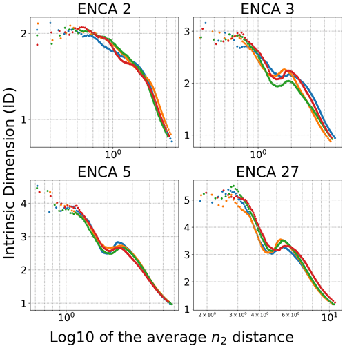
Figure A1 GRIDE evolution plot for the different ENCA models employed for the four random restarts of the models.

In order to estimate the ID, we apply the GRIDE estimator (Denti et al., 2022). Given sample points x_i∈ℝ^D, for $i=\mathrm{1},\mathrm{\dots },M$, and a distance measure, $r:{\mathbb{R}}^D\times {\mathbb{R}}^D\to {\mathbb{R}}^{+}$, GRIDE assumes that points in a given neighbourhood are counted with a Poisson point process with intensity ρ, which is constant at least up to the scale of the diameter of the considered neighbourhood. Let r_i,l be the distance between the point x_i and its lth nearest neighbour and define ${\mathit{\mu }}_{i,n_{\mathrm{2}},n_{\mathrm{1}}}=\frac{r_{i,n_{\mathrm{2}}}}{r_{i,n_{\mathrm{1}}}}$, where n₁ and n₂ (with $\mathrm{0}\le n_{\mathrm{1}}\le n_{\mathrm{2}}\le M$) are the given integers. The distribution of ${\mathit{\mu }}_{i,n_{\mathrm{2}},n_{\mathrm{1}}}$ can be computed in closed form and depends only on the ID of the data while, crucially, not depending on ρ, as long as ρ is constant in the considered neighbourhood of i, whose diameter is set by the distance between i and its n₂th nearest neighbour (Denti et al., 2022).

In order to correctly identify the ID of a dataset, a scale-independent analysis is essential. We therefore make use of GRIDE paths, the evolution of the ID estimate as a function of n₂, which can be interpreted as the scale at which we look at the data. We set $n_{\mathrm{1}}=n_{\mathrm{2}}/\mathrm{2}$, as is usually done in the literature. As a function of n₂, the ID is first expected to decrease after a maximum due to the noise present at small distance scales, and then reach a plateau corresponding to the correct ID.

Figure A1 shows the GRIDE path for the different ENCA models trained in this work. In particular, the ID estimate of the latent space of ENCA-27 decreases after showing a plateau around five, then reaches a minimum around three, then increases again, and finally collapses to low values at a larger distance scale. The plateau at five motivates us to train ENCA-5 and study its ID. The local minimum of the GRIDE path of the latent space of ENCA-5 is consistent with an ID of three. We can deduce that, for most of the catchments, the ID is three, while for some it can be higher. However, the fact that the GRIDE path of the latent space of ENCA-27 shows two plateaus around five and three can be an indicator of the existence of two or more manifolds with different IDs. From Fig. 3 we see that, indeed, three features seem to capture most of the relevant information, which is in line with the GRIDE path for ENCA-5.

Appendix B: Metric comparisons

We report some summary statistics of the NSE, R, BIAS, and SD values across the 568 catchments considered in this study. In terms of the linear correlation coefficient R and BIAS (left and central panels of Fig. B1), we observe a similar pattern to what we observed for the NSE distribution (Fig. 3). By increasing the number of latent features to three, the bulk distribution improves significantly. At the same time, further increasing the number of latent features only improves the BIAS outliers. Regarding the SD (right panel of Fig. B1), it is clear that both the CAAM and ENCA models tend to underestimate the streamflow variability, a known issue associated with using NSE as the objective function (Gupta et al., 2009). However, the differences between the CAAM and ENCA models are less pronounced, and, unlike the observations for NSE, R, and BIAS, a clear performance hierarchy cannot be established.

Figure B1 R, BIAS, and SD values for the considered models in the test period. The boxes are delimited by the 25 % and 75 % quantiles, while the whiskers indicate the 5 % and 95 % quantiles. For these metrics, the CAAM performance is similar to that of ENCA-2.

Table B1 demonstrates that increasing the number of latent features in ENCA generally enhances performance. However, the improvement is modest between ENCA-3 and ENCA-5 and nearly negligible between ENCA-5 and ENCA-27. The performance of CAAM is more comparable to ENCA-2 overall, suggesting that the third latent feature is crucial for better predictions in certain catchments, while five features appear to be the maximum number that our encoder can effectively learn. Furthermore, as shown in Fig. 5, it is clear that almost all catchments that improved from ENCA-3 to ENCA-5 still exhibit very poor performance (NSE below −1.0).

Table B1 Metric comparison for the different models computed in the test period. We report the mean, minimum, 5 % quantile, 25 % quantile, median, 75 % quantile, 95 % quantile, and maximum values. Additionally, we report the number of catchments whose predicted NSE values are lower than zero.

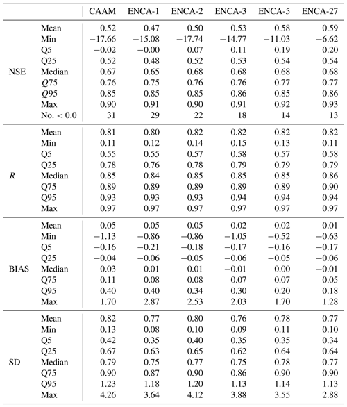
Table B2 Linear correlation coefficients between the different metrics in the models analysed in this work. Catchments whose NSE prediction is lower than zero are excluded.

From Table B2, we can observe that the NSE is strongly correlated with the linear coefficient R and fairly correlated with SD, and the correlation increases with the performance (see Fig. 3). At the same time, the NSE is anti-correlated with BIAS, but this correlation is low. While the correlations between R and BIAS and between BIAS and SD are weak, the correlation between R and SD is intermediate and increases with performance. These results agree with the findings of Gupta et al. (2009), who showed that, with optimal BIAS values, optimal NSE values are reached when R is correlated with SD.

Appendix C: Neural network details and training losses

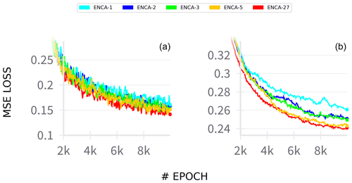
Figure C1 Training MSE loss (a) and test loss (b) during training for the different ENCA models. The curves shown are obtained by averaging the losses across different random restarts. The loss variability across the random restarts (not shown) is negligible.

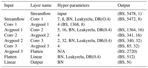
We report the architecture details of the encoder (Table C1) of the ENCA models used in this work. For the encoder, we chose a single-layer unidirectional LSTM, followed by a dropout layer (with probability 0.4) and a fully connected layer that maps the LSTM output layer to the predicted output. For the LSTM, we chose a hidden size of 256 (number of memory cells) and an initial forget bias of 5.

Table C1 The convolutional encoder architecture used in this study. Batch normalization (BN) and dropout (DR) with probability 0.4 are added among the layers. A last BN layer is applied to the decoder output in order to standardize the latent features. N is the number of latent features. The batch size is indicated with “BS”.

In Fig. C1 we report the training and test losses of some models that were employed. We observe that all of the employed models are about to reach a plateau where the test loss no longer decreases. Though convergence is not perfectly reached due to computational limitations, the fact that the test loss is almost at the reachable minimum is an indicator that the models are not overfitting the dataset.

Additionally, we report the mean and standard deviations of the latent features of ENCA-5 (Table C2). We can appreciate a small amount of bias, even if the encoder succeeds in preserving the standard deviation of the latent features close to 1. We found similar behaviour in the latent features of other ENCA models (not reported).

Table C2 Mean and standard deviation of the latent features of ENCA-5.

Appendix D: Known attributes and signature correlation

Figure D1 Absolute Spearman correlation matrix of the selected catchment attributes and hydrological signatures with one another.

Appendix E: Effect of random restart

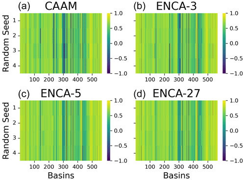
Figure E1 Test NSE values of four random restarts for CAAM (a), ENCA-3 (b), ENCA-5 (c), and ENCA-27 (d) for the 568 catchments considered in this study. NSE values are clipped in the interval $[-\mathrm{1},\mathrm{1}]$. We do not observe much performance variability across the different random restarts.

We ascertain that random restart does not affect the prediction accuracy much (Fig. E1). Apart from some catchments, most of them show consistent behaviour across different random seeds.

We report the correlation matrix between the principal components of the learnt features of ENCA-5 (Fig. E2) and ENCA-27 (Fig. E3) for different random restarts. We notice a consistency across random restarts and different models. Moreover, the correlation becomes weaker and weaker with the fourth component, indicating that three features carry most of the information related to streamflow prediction.

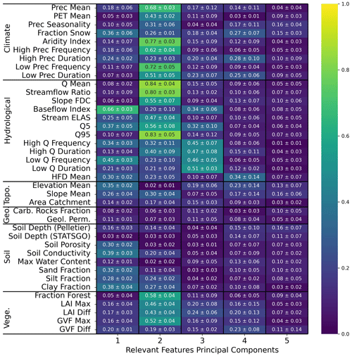
Figure E2 Average (plus or minus the standard deviation) of the absolute Spearman correlation of the relevant feature principal components of ENCA-5 with respect to the catchment attributes and hydrological signatures across the four different random model restarts. The colours refer to the average.

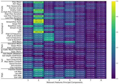
Figure E3 Average (plus or minus the standard deviation) of the absolute Spearman correlation of the relevant feature principal components of ENCA-27 with respect to the catchment attributes and hydrological signatures across the four different random model restarts. The colours refer to the average. For a better visualization, we only report the first eight principal components.