Identification, mapping, and eco-hydrological signal analysis for groundwater-dependent ecosystems (GDEs) in Langxi River basin, north China

Groundwater-dependent ecosystems (GDEs) refer to ecosystems that require partial or complete access to groundwater to maintain their ecological structure and functions, providing very important services for the health of land, water, and coastal ecosystems. However, regional identification of GDEs is still difficult in areas affected by climate change and extensive groundwater extraction. To address this issue, taking the Langxi River basin (LRB), one of the lower tributaries of the Yellow River in north China, as an example, we propose a four-diagnostic-criteria framework for identifying the GDEs based on remote sensing, geographic information system (GIS) data dredging, and hydrogeological survey data. Firstly, the potential GDE distributions are preliminarily delineated by the topographic features and the differences in terms of vegetation water situation and soil moisture at the end of the dry and wet seasons. On this basis, according to the given GDE identification criteria, three main types of GDEs in the basin, including the stream-type GDEs (S-GDEs), vegetation-type GDEs (V-GDEs), and karst-aquifer-type GDEs (K-GDEs), are further determined by comparing the relationship between groundwater table, riverbed elevation, and vegetation root development depth and through surveys of karst springs and aquifers. Following this, the GDEs are mapped using the spatial kernel density function, which can represent the characteristics of spatial aggregation distribution. Results show that the potential GDEs are mainly distributed in plain areas, with a small part in hilly areas, reflecting the moisture distribution status of waters, vegetation, and wetlands in the basin that possibly receive groundwater recharge; however, the true GDEs are concentrated in the riverine and riparian zone, the vegetation-related wetland, and the scattered karst spring surroundings which groundwater directly moves toward and into. In order to verify the reliability of GDE distributions, the study verified the determination of GDEs through hydrological rhythm analysis, as well as through the analysis of the hydrochemical characteristics of various waterbodies in the basin and of ecohydrological signals such as groundwater invertebrates. The hydrological rhythm analysis in the Shuyuan section showed that the proportion of base flow to river flow is about 54.15 % and that S-GDEs still receive spring water recharge even in the extremely dry season. Furthermore, the analysis of hydrochemical sampling from the karst aquifer, the Quaternary aquifer, the spring water, and the surface reservoir water reveals that GDEs are also relished by groundwater. More importantly, we also found a distinctive ecohydrological signal of GDEs is the presence of millimeter-sized groundwater fauna living in the different types of GDEs. In addition, the study suggests that the use of isotope and environmental DNA technology to analyze the hydrological–sediment–biological connectivity between groundwater and GDEs is the future development direction of this field.

1 Introduction

In the area where surface water interacts with groundwater, due to the temporal and spatial differences in precipitation, infiltration, recharge, runoff, and other processes, an ecosystem is formed around low-lying land, riverbanks on both banks, and karst caves. This is due to temporal and spatial differences in precipitation, infiltration, recharge, runoff, and other processes (Bowles and Arsuffi, 1993; Rohde et al., 2017). Early scholars referred to this ecosystem as “groundwater-fed wetland” or “groundwater-dominated stream ecosystems” (Eamus and Froend, 2006; Gilvear et al., 1993; Petts et al., 1999). Australian scholars proposed the concept of “groundwater-supported ecosystems” or “groundwater-dependent ecosystems” (GDEs for short) earlier, with a focus on the water requirements of plants (Clifton and Evans, 2001; Hatton et al., 1997). These ecosystems have distinct characteristics that are closely related to groundwater on a continuous basis and may also be seasonally or occasionally dependent on it (Foster et al., 2006). The composition, structure, and function of GDEs are influenced by groundwater through flow, nutrient recharge, and pressure and water temperature transport. Additionally, the biological processes of GDEs, such as plant photosynthesis, microbial action, and animal activities, can impact surface water–groundwater hydrological processes, including surface water evaporation, flow, groundwater seepage, and recharge (Boulton et al., 2003; Murray et al., 2003; Schenková et al., 2018). GDEs not only sustain the health of ecosystems but also mitigate the effects of floods and droughts while providing essential products and services, such as food production and water purification, to humans. Consequently, enhancing their protection and management is of vital ecological, social, and economic significance.

Scholars have classified GDEs in numerous ways over the years. In 1997, Hatton et al. (1997) proposed a classification system for Australia's GDEs based on their reliance on groundwater, dividing them into four categories: wetlands and terrestrial GDEs, mound spring ecology GDEs, aquatic GDEs, and aquifer and cave GDEs. Building on the Hatton et al. (1997) classification system, Clifton and Evans (2001) introduced two additional types of GDEs, terrestrial-fauna GDEs and estuarine and near-shore marine GDEs, based on the spatial distribution of GDEs in land and estuary areas. In later studies, Eamus and Froend (2006) simplified the six classifications into three (groundwater ecosystems, ecosystems dependent on belowground expression of groundwater, and ecosystems dependent on aboveground expression of groundwater), while Bertrand et al. (2012) argued that, as a result of climate change, it is necessary for GDEs to define potential GDE ecosystems that can account for the full spectrum of GDEs under varying climatic conditions. The Global Water MATE Core Group, the World Bank, and the United States Department of Agriculture's (USDA) National Agricultural Statistics Service (NASS) guidelines have classified GDEs based on differences between arid, humid, coastal, and inland areas (Foster et al., 2006). As evident from the aforementioned guidelines, the classification of GDEs varies across different research regions and environments. Therefore, defining the appropriate classification of GDEs is crucial in accurately identifying and distributing them in the study area.

GDEs are vulnerable to disturbances caused by both natural and human activities (Dong and Zhang, 2011; van Engelenburg et al., 2018). Natural factors that affect GDEs include climate change, topography, and hydrogeological conditions. Human activities that affect GDEs include changes in underlying surface conditions, habitat environment disturbances, water conservancy construction, and groundwater exploitation. The impact of climate change and groundwater exploitation on GDEs has garnered increasing attention, and some scholars have conducted multi-factor impact assessments and risk analyses to better understand their effects. According to Humphreys (2006), aquatic vegetation is closely linked with groundwater ecosystems. Laio et al. (2009) developed a conceptual model to illustrate the relationships among rainfall, groundwater level, and vegetation in the GDEs. Their model indicated that the stochastic, dynamic changes in groundwater level are closely tied to climate change, vegetation coverage, and water resource management levels. Hancock and Boulton (2009) conducted multidisciplinary research on aquifers, hydrogeology, ecology, and the relationship between groundwater and its associated ecosystems. They noted that surface vegetation is also influenced by groundwater processes, which are crucial to consider when studying GDEs, particularly in water-limited environments.

Identifying and mapping GDEs in the wild can be challenging, particularly in areas heavily impacted by human activities, despite their widespread distribution. Early studies primarily utilized field hydrogeological and ecological survey techniques to determine GDEs. For instance, Eamus and Froend (2006) suggested a toolbox comprising various methods to identify GDEs and their reliance on groundwater, as well as vegetation processes dependent on groundwater, based on the type of GDE. With the widespread adoption and application of remote sensing and geographic information system (GIS) methods, researchers have been able to analyze spatial data with greater precision. For example, Howard and Merrifield (2010) utilized GIS methods to study California, USA, and to establish a groundwater dependency index. By doing so, they were able to identify, map, and classify various types of groundwater-dependent ecosystems (GDEs) such as springs, wetlands, and streams into different dependency levels. Hoogland et al. (2010) evaluated the dry water shortage of GDEs in the Netherlands by creating groundwater depth maps. Lastly, Gou et al. (2015) were the first to use GIS database information to determine the potential distribution of GDEs at a state or province level. To track and identify changes in vegetation pixels, researchers often use Landsat imagery to analyze the normalized difference vegetation index (NDVI), which helps to determine the distribution of groundwater-supported vegetation at the aquifer or basin scale. While traditional hydrogeological surveys can be time-consuming and expensive, remote sensing methods provide an efficient way to determine large-scale GDE distributions. However, remote sensing may not always be accurate at small scales, such as at the segment scale of river sections. Therefore, combining traditional hydrogeological surveys, field ecological monitoring, global positioning systems (GPSs), GISs, and remote sensing (RS) is an effective method for identifying and mapping GDEs.

To improve the identification and mapping of GDEs, it is important to analyze their ecohydrological characteristics. This involves studying the interaction process between surface water and groundwater, as well as the simulation of material transport, to determine the regional ecohydrological characteristics. These characteristics can often be regarded as a specific signal for monitoring ecosystem status and linking the functions of organisms to ecohydrological processes, such as the rhythm of hydrometeorological elements, hydrogeochemical characteristics, and biological indicators (just like biodiversity, connectivity, etc.). Understanding these characteristics can help determine if there is hydrological connectivity between groundwater and potential GDEs and whether a “hydrological continuum” can be formed. This is crucial for maintaining the integrity of the system and the ecological processes regulated by the “ecotones”. Hao et al. (2018) found that, although groundwater development has weakened the relation between spring discharge and precipitation, the resonant frequency between spring discharge and precipitation remained unchanged when studying the discharge data of Niangziguan spring, a karst hydrological case in north China. Brancelj et al. (2020) provided an overview of groundwater fauna in the phreatic zone of the Classical Karst aquifer and discovered that the rate of endemism within the area is very high (around 50 %); this can be considered to be a descriptor of the aquifer type and habitat structure, as well as of the water flow regime and groundwater flow paths. These case studies are examples of unique ecohydrological habitats that are an essential part of global research. In addition, the ecohydrological process of GDEs is also demonstrated through the hydrological and hydraulic connections between the vegetation ecosystem and precipitation, surface water, and groundwater. Therefore, analyzing the ecohydrological characteristics of GDEs can provide valuable insights into their functioning and can help in their effective management and conservation. Moreover, what sets GDEs apart from other ecosystems is the unique presence of groundwater invertebrate fauna, spanning from millimeters to centimeters, which serve as crucial indicator species for groundwater-supported ecosystems. Therefore, conducting sampling and species identification, assessing the biodiversity and ecology of groundwater faunas, and zoning animal habitats are all essential components of GDE researches. From the above analysis, it can be seen that the research on the distribution of GDEs is still in the initial stage of exploration, and the research methods are not the same. It is urgent to put forward a comprehensive and applicable research theory.

The author provided a comprehensive summary of research on GDEs (Li et al., 2018), revealing that there is limited research that has been conducted in China, with most studies focusing on the hyporheic zone, karst ecotone, northwestern grassland, desert oasis, and other regions. Furthermore, the overexploitation of groundwater in northern China has resulted in the shrinking of GDEs over a large area, making identification and mapping challenging. The Langxi River basin (LRB) is situated on the southern bank of the Yellow River, on the north side of Mount Tai, and is part of a vast carbonate distribution area. The region is also located in the western part of Jinan City, where many springs have developed, giving rise to various types of GDEs, which are typical of northern China. Thus, the purpose of this study is to identify the types of GDEs affected by human activities and to delineate their scope to improve the basis for regional water resources planning and karst spring protection. The study has three primary objectives: first, to propose a criteria framework for identifying, mapping, and verifying GDEs; second, to identify and map the distribution of GDEs in a typical study basin using the soil-moisture-based remote sensing method and the spatial kernel density function; and, third, to verify the reliability of GDE zoning through ecohydrological signal analysis in the river basin.

2 Materials and methods

2.1 Study area

The Langxi River basin (LRB) is a typical karst basin situated in the southwest of Jinan, China, spanning an area of 137.8 km², with a river length of 26.68 km. It is one of the lower tributaries of the Yellow River (Fig. 1). The LRB is characterized by a continental monsoon climate, with an average annual rainfall of 604 mm, which mainly falls during the summer season. Precipitation from June to August contributes to 65 % of the total annual rainfall. Consequently, the runoff of the Langxi River is highly unstable, with maximum flow reaching 159 m³ s⁻¹ during the flood season and with a risk of no flow during the dry season. In order to optimize water usage, small reservoirs and dams have been constructed in the upper and middle reaches of the river for irrigation purposes. The number of surface water resources and groundwater resources and the amount of exploitable groundwater in the LRB equate to 11.5×10⁶ m³, 24.82×10⁶ m³, and 20.75×10⁶ m³, respectively. There are two aquifers in the study area: one is the Quaternary pore water aquifer, which is regarded to be an unconfined aquifer, and the second is the Cambrian karst aquifer, which is regarded to be a confined aquifer.

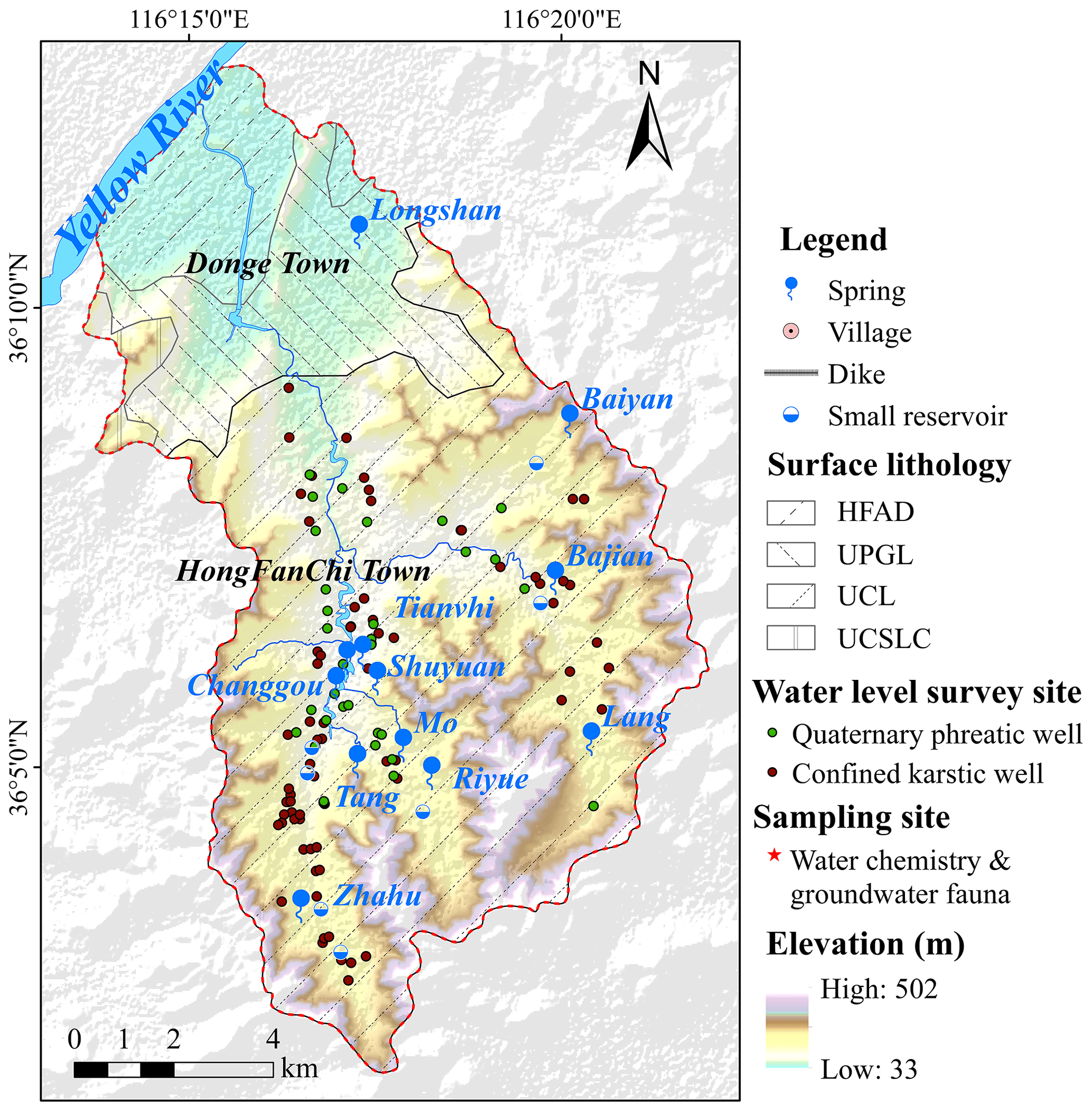
Figure 1 The location, lithology, topography, spring water, groundwater-level survey points, and hydrochemical groundwater biological sampling points of the Langxi River basin. HRAD: Holocene fluvial alluvial deposits, UPGL: Upper Pleistocene gravel layer, UCL: Upper Cambrian limestone, UCSLA: Upper Cambrian shale–limestone amalgamation.

The southern region of the LRB is characterized by a higher elevation and is enclosed by mountains. The valley is positioned in the central area and predominantly comprises low hills and plains, with an average elevation ranging from 100 to 250 m. The lowest point within the basin is located at the confluence of the Langxi River and the Yellow River, with an altitude of 36 m. The valley is home to diverse vegetation such as swamp, meadow, riparian sparse forest, and shrubs, creating distinct habitat landscapes along the river course.

The Cambrian and Quaternary strata are widely distributed throughout the basin, with the surface lithology consisting of hard limestone, the Cambrian Zhangxia Group, a Quaternary alluvial accumulation layer, and river–lake facies sandy clay and gravel. The water-bearing rock group comprises the Quaternary loose porous rock aquifer and the Cambrian carbonate fissure karst aquifer. Due to differences in topography and geology, various rising and descending springs are formed across different regions. The piedmont fault zones and areas with thin Quaternary sediments are rich in karst springs, resulting in wetlands of different sizes and scenic landscapes. According to historical records, there are 34 springs in the basin. Riparian zones and wetlands with shallow groundwater support GDEs through groundwater seepage and karst springs. Based on GIS data and survey results, a hydrogeological profile was constructed perpendicularly to the Langxi River and Shuyuan spring (Fig. 2). The reason for selecting this section is that it contains the three types of GDEs defined in this study and is therefore significantly representative in the LRB. The Shuyuan spring, located at the junction of the Quaternary and Cambrian strata, is formed in the Cambrian Oolitic limestone of the Zhangxia Group, which has well-developed karst fissures in the east. The groundwater head is approximately 20 m higher than the surface, resulting in an artesian descending spring.

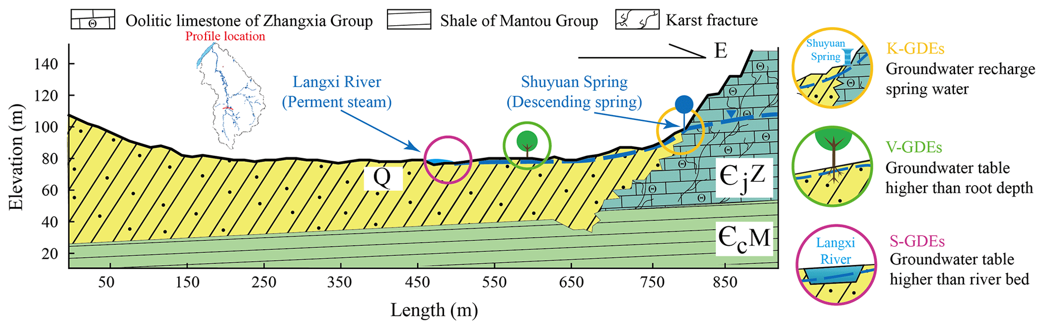
Figure 2 Hydrogeological profile of Shuyuan spring in the LRB. The dotted line shows the characteristics of the water table in the geological section. The geological types in the figure are Q (Quaternary sedimentary layer), ϵ_jZ (Cambrian Zhushadong–Zhangxia Formation limestone), and ϵ_cM (Cambrian Gushan–Chaomidian Formation limestone).

2.2 Framework for identification, mapping, and verification of GDEs

This paper identifies GDEs in the LRB based on the aforementioned GDE classification and the actual situations. Four criteria are used to identify GDEs:

1. Karst springs and associated wetlands. These ecosystems include karst springs, groundwater seeps, sinkholes, karst aquifers, and wetlands formed around karst springs or fed directly by karst groundwater. Collectively, they are referred to as karst-groundwater-dependent ecosystems (K-GDEs).

2. Gaining streams. These are streams or parts of streams where flow is solely or partly contributed by inflow of groundwater. Typically, the groundwater table is at or above the stream level and moves toward and into the river, forming a stream-related ecosystem.

3. River riparian zone. This zone is adjacent to gaining streams and is characterized by distinctive plant and animal communities that are directly or indirectly fed by groundwater. The above two GDEs are mainly distributed in the river and on both sides of the river and are referred to as stream-type GDEs (S-GDEs).

4. Vegetation-related ecosystems. These ecosystems are home to vegetation that grows in areas with shallow groundwater tables that roots may access to store water or where the vegetation types are considered to be phreatophyte species. These types of ecosystem typically maintain greenery even during extremely dry periods and are referred to as vegetation-type GDEs (V-GDEs).

Using these four identified criteria, we propose a diagnostic framework for data collection and the identification, mapping, and verification of GDEs in the LRB (Fig. 3).

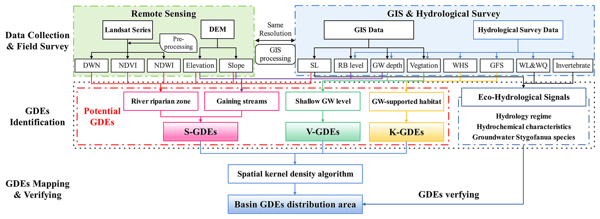
Figure 3 Diagnostic framework for GDE identification, mapping, and verification. Note: DEM refers to digital elevation model; DWN refers to the difference between the wet index and the normalized difference built up and the soil index; GIS refers to geographic information system; SL refers to surface lithology; RB refers to riverbed; GW refers to groundwater; WHS refers to water hydrochemical sampling; GFS refers to groundwater fauna sampling; WL and WQ refers to water level and water quality; S-GDEs refers to stream-type GDEs; V-GDEs refers to vegetation-type GDEs; and K-GDEs refers to karst-type GDEs.

2.3 Identification and mapping of GDEs

2.3.1 Potential GDE quantification

Groundwater collection places are typically found on level plains or in low-lying valleys. To make these regions easier to locate, lowlands and mountains have been divided. First, using a digital elevation model (DEM) and the slope (calculated by the DEM), we can distinguish the plains and hills of the basin (Eq. 1) and can further divide the plains of shallow fissure rocks according to the surface lithology, which is the area with the conditions for the formation of GDEs.

$$\begin{array}{}\text{(1)}& {\mathrm{grid}}_{\mathrm{plain}}={\mathrm{grid}}_{\left(\mathrm{slope}\le {\mathrm{\Delta }}_{\mathrm{slope}}\right)\cap \left(\mathrm{elevation}\le \stackrel{\mathrm{‾}}{\mathrm{elevation}}\right)}\end{array}$$

In the above, grid_plain represents the grid divided into plains, and Δ_slope is the threshold of the maximum plain slope; in this paper, we take Δ_slope=10°. The determination of this parameter can be manually adjusted based on one-third of the average slope of the basin until the plains and mountains are clearly distinguished (see Fig. S3 in the Supplement). $\stackrel{\mathrm{‾}}{elevation}$ is the average elevation of the basin. When applying this method in a basin with a significant difference in elevation, we highly recommend adjusting the value instead of simply using the average value.

Previous studies utilized Eqs. (2) and (3) to calculate the normalized difference vegetation index (NDVI) and the normalized waterbody index (NDWI), respectively, from infrared optical remote sensing Landsat satellite data. These indices were then used at the end of the wet and dry seasons to distinguish the rate of vegetation loss due to water and to identify the extent of GDEs. Due to the difficulty of obtaining a clear NDWI image in the study area (Fig. S1), we opted to enhance our method by utilizing the more discriminative difference between the WET index and the normalized difference built-up and the soil index (NDBSI). The WET and NDBSI indices represent regional humidity and dryness, respectively. The two indices are the average values derived from multiple images captured during both the dry and wet seasons within a year. Additionally, the two largest sources of water supply, apart from precipitation, are the lateral input of groundwater and rivers, which are dependent on the surface lithology of the basin. The difference between the two indices can be used to calculate the extreme variation in dryness and humidity in a specific region over a given period, thereby reflecting the average water reserves in that quarter. This is particularly relevant in areas such as river riparian zones, which are located near gaining streams and are characterized by distinct vegetation that remains green even during extremely dry periods. The potential GDE distribution area can be determined by establishing a critical threshold (δ_WD) of the difference. The equations (Eqs. 2 to 6) below illustrate the indices and methodology for assessing the distribution area of potential GDEs (Gao, 1996; Karbalaei Saleh et al., 2021; Pettorelli et al., 2005):

$$\begin{array}{}\text{(2)}& {\displaystyle }\mathrm{NDVI}={\displaystyle \frac{{\mathit{\rho }}_{\mathrm{nir}}+{\mathit{\rho }}_{\mathrm{red}}}{{\mathit{\rho }}_{\mathrm{nir}}-{\mathit{\rho }}_{\mathrm{red}}}},\text{(3)}& {\displaystyle }\mathrm{NDWI}={\displaystyle \frac{{\mathit{\rho }}_{\mathrm{nir}}+{\mathit{\rho }}_{\mathrm{swir}\mathrm{1}}}{{\mathit{\rho }}_{\mathrm{nir}}-{\mathit{\rho }}_{\mathrm{swir}\mathrm{1}}}},\text{(4)}& {\displaystyle }\begin{array}{rl}\mathrm{WET}& =c_{\mathrm{1}}\cdot {\mathit{\rho }}_{\mathrm{blue}}+c_{\mathrm{2}}\cdot {\mathit{\rho }}_{\mathrm{green}}+c_{\mathrm{3}}\cdot {\mathit{\rho }}_{\mathrm{red}}+c_{\mathrm{4}}\cdot {\mathit{\rho }}_{\mathrm{nir}}\\ & +c_{\mathrm{5}}\cdot {\mathit{\rho }}_{\mathrm{swir}\mathrm{1}}+c_{\mathrm{6}}\cdot {\mathit{\rho }}_{\mathrm{swir}\mathrm{2}},\end{array}\text{(5)}& {\displaystyle }\mathrm{NDBSI}={\displaystyle \frac{\mathrm{IBI}+\mathrm{SI}}{\mathrm{2}}}={\displaystyle \frac{\begin{array}{c}\frac{\frac{\mathrm{2}{\mathit{\rho }}_{\mathrm{swir}\mathrm{1}}}{{\mathit{\rho }}_{\mathrm{swir}\mathrm{1}}+{\mathit{\rho }}_{\mathrm{nir}}}-\left[\frac{{\mathit{\rho }}_{\mathrm{nir}}}{{\mathit{\rho }}_{\mathrm{nir}}+{\mathit{\rho }}_{\mathrm{red}}}+\frac{{\mathit{\rho }}_{\mathrm{green}}}{{\mathit{\rho }}_{\mathrm{green}}+{\mathit{\rho }}_{\mathrm{swir}\mathrm{1}}}\right]}{\frac{\mathrm{2}{\mathit{\rho }}_{\mathrm{swir}\mathrm{1}}}{{\mathit{\rho }}_{\mathrm{swir}\mathrm{1}}+{\mathit{\rho }}_{\mathrm{nir}}}+\left[\frac{{\mathit{\rho }}_{\mathrm{nir}}}{{\mathit{\rho }}_{\mathrm{nir}}+{\mathit{\rho }}_{\mathrm{red}}}+\frac{{\mathit{\rho }}_{\mathrm{green}}}{{\mathit{\rho }}_{\mathrm{green}}+{\mathit{\rho }}_{\mathrm{swir}\mathrm{1}}}\right]}\\ +\frac{\left[\left({\mathit{\rho }}_{\mathrm{swir}\mathrm{1}}+{\mathit{\rho }}_{\mathrm{red}}\right)-\left({\mathit{\rho }}_{\mathrm{nir}}+{\mathit{\rho }}_{\mathrm{blue}}\right)\right]}{\left[\left({\mathit{\rho }}_{\mathrm{swir}\mathrm{1}}+{\mathit{\rho }}_{\mathrm{red}}\right)+\left({\mathit{\rho }}_{\mathrm{nir}}+{\mathit{\rho }}_{\mathrm{blue}}\right)\right]}\end{array}}{\mathrm{2}}},\text{(6)}& {\displaystyle }{\mathrm{grid}}_{\mathrm{potenial}\mathrm{GDEs}\mathrm{area}}={\mathrm{grid}}_{\left(\left(\mathrm{WET}-\mathrm{NDBSI}\right)\le {\mathit{\delta }}_{\mathrm{WD}}\right)},\end{array}$$

where c₁ to c₆ are sensor parameters. Due to the different types of sensors, the parameters are also different. See Table S1 for specific parameters. IBI and SI are the building index and soil index. ρ_red, ρ_green, ρ_blue, ρ_nir, ρ_swir1, and ρ_swir2 are the red band, green band, blue band, near-red band, mid-infrared band 1, and mid-infrared band 2, respectively. The δ_WD is the threshold used to demarcate the boundaries of potential GDE distribution regions, which is determined by a trial-and-error algorithm. In this paper, we take δ_WD=0.3.

Table 1 Remote sensing and hydrogeological survey data used in the research.

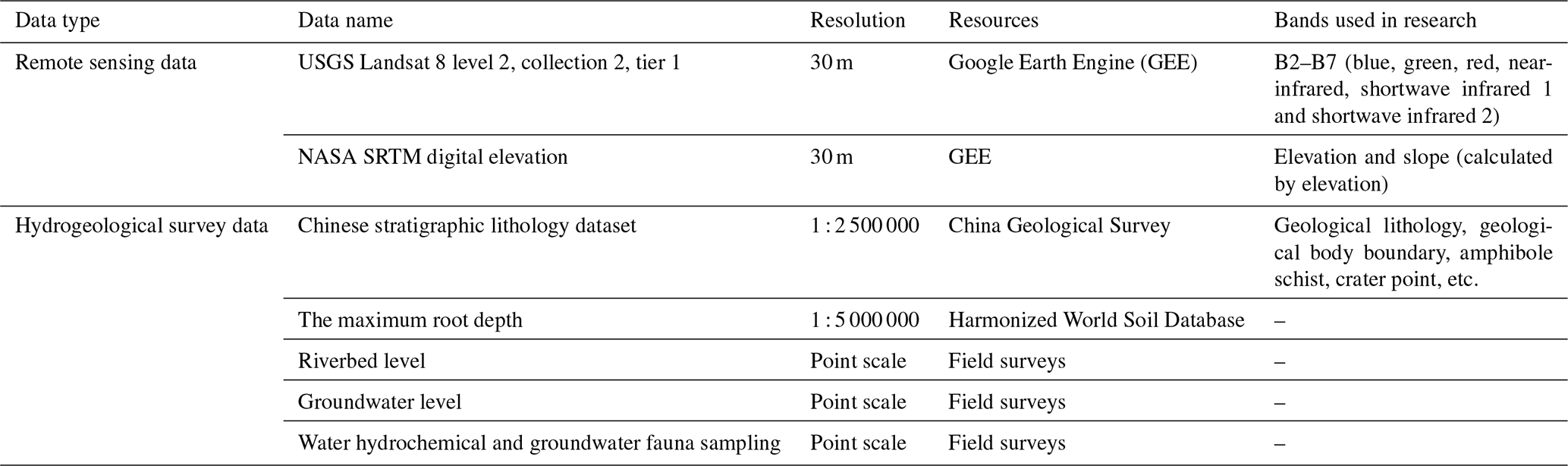
Note: please see Table S2 for remote sensing data sources.

Modified by the GDE mapping (GEM) method proposed by Barron et al. (2014), the potential GDEs are based on vegetation and moisture responses observed at the surface during an extended dry period. It is assumed that soil moisture would be depleted due to minimal rainfall over a 6- to 7-month drought, and areas with consistent greenness and high surface wetness were more likely to have access to groundwater. Based on remote sensing indices, various regions can be categorized into different groups, such as permanent open waterbodies, slow-drying vegetation, fast-drying vegetation, and crops. The permanent open waterbodies exhibit consistently high wetness and consistently low greenness throughout the dry season. In contrast, the slow-drying vegetation tends to display some level of reduction in both greenness and wetness after an extended dry period, typically caused by a decrease in groundwater contribution to base flow or annual groundwater table subsidence. The fast-drying vegetation, where the root zone is frequently disconnected from groundwater, may experience a significant decline in surface greenness and wetness due to the complete exhaustion of soil moisture stores at the end of a long dry period. Lastly, crop areas can be distinguished by discernible changes in planting and harvesting seasons.

By using riverbed and Quaternary water level data, it is possible to identify gaining streams, where the Quaternary water level is higher than the elevation of the riverbed, allowing groundwater to flow laterally and to supply vegetation in the subsurface with water either seasonally or year-round. The areas where vegetation directly receives groundwater recharge can be determined by taking into account the vegetation root depth and the Quaternary water level. These areas are referred to as V-GDEs. The riparian buffer zone of the river, which is nourished by groundwater, partially overlaps with these areas and is classified as an S-GDE.

By conducting field investigations and analyzing samples from karst springs and the surrounding environment, it is possible to define the distribution area of K-GDEs in the basin. Additionally, unique water chemistry and aquatic biological characteristics obtained through sampling, as well as changes in the surface vegetation and ecological environment recorded during the survey, can provide supporting evidence for the delineation of K-GDEs.

2.3.2 GDE mapping

By applying the four diagnostic criteria, we are able to pinpoint the grids or ranges that are classified as GDEs. In this paper, we utilize the spatial kernel density algorithm to conduct a probability density partitioning of the distribution range of GDEs within the basin. The fundamental concept behind kernel density estimation is that each data point within the space will have an impact on a particular area through the density function. By constructing a spatial kernel density function model, we can determine the impact of any location within a given sample space (Cai et al., 2013; Hallin et al., 2004). This allows us to estimate the probability distribution of GDEs in our study. Kernel density estimation is a non-parametric technique used to estimate a probability density function. The kernel density at the coordinates (x,y) can be calculated using Eq. (7):

$$\begin{array}{}\text{(7)}& \begin{array}{rl}{\mathrm{density}}_{\left(x,y\right)}& ={\displaystyle \frac{\mathrm{1}}{{\left(\mathrm{radius}\right)}^{\mathrm{2}}}}\\ & {\sum }_{i=\mathrm{1}}^n\left[{\displaystyle \frac{\mathrm{3}}{\mathit{\pi }}}\cdot {\mathrm{pop}}_i{\left(\mathrm{1}-{\left({\displaystyle \frac{{\mathrm{dist}}_i}{\mathrm{radius}}}\right)}^{\mathrm{2}}\right)}^{\mathrm{2}}\right]\\ & ,{\mathrm{dist}}_i<\mathrm{radius},\end{array}\end{array}$$

where $i=\mathrm{1},\mathrm{2},\mathrm{\dots },n$ is the input point. We only include points in the sum if they are within a radial distance of the (x,y) location. pop_i is the population field value for point i, which is an optional parameter; in this paper, we define pop_i=1. dist_i is the distance between point i and the (x,y) position. The term radius refers the search radius in Eq. (8), also known as the bandwidth. In this paper, the method for calculating bandwidth for the two adjacent grids is defined by taking the smaller value between the unweighted standard distances (Eq. 9) and the second term of the min function in Eq. (8).

$$\begin{array}{}\text{(8)}& {\displaystyle }\mathrm{SearchRadius}=\mathrm{0.9}\times min\left(\mathrm{SD},\sqrt{{\displaystyle \frac{\mathrm{1}}{\ln \left(\mathrm{2}\right)}}}\times D_{\mathrm{m}}\right)\times n^{-\mathrm{0.2}}\text{(9)}& {\displaystyle }\mathrm{SD}=\sqrt{{\displaystyle \frac{{\sum }_{i=\mathrm{1}}^n{\left(x_i-\stackrel{\mathrm{‾}}{X}\right)}^{\mathrm{2}}}{n}}+{\displaystyle \frac{{\sum }_{i=\mathrm{1}}^n{\left(y_i-\stackrel{\mathrm{‾}}{Y}\right)}^{\mathrm{2}}}{n}}+{\displaystyle \frac{{\sum }_{i=\mathrm{1}}^n{\left(z_i-Z\right)}^{\mathrm{2}}}{n}}}\end{array}$$

In the above, D_m is the (weighted) median distance from the (weighted) mean center. SD is the standard distance.

By selecting a non-fixed bandwidth that varies based on the estimated location (balloon estimator) or sample points (pointwise estimator), we can utilize a powerful approach known as adaptive or variable bandwidth kernel density estimation. This method enables us to provide a more accurate depiction of the spatial distribution characteristics of GDEs.

2.4 Verifying GDEs using eco-hydrological signal analysis

By extracting and refining the eco-hydrological features of the basin, the eco-hydrological signal can be obtained, and the discriminant range of GDEs can be verified. This paper selects three types of eco-hydrological signals: base flow recharge of groundwater to karst springs, hydrochemical characteristics of various waterbodies in the basin, and groundwater fauna.

2.4.1 Hydrographic analysis: base flow signals

The base flow recharge of groundwater to karst springs can demonstrate that the karst aquifer in the watershed can replenish the surrounding ecosystem through surface runoff formed by spring water. The primary objective of the hydrological analysis method is to analyze and validate the proportion of groundwater recharge through base flow signals in S-GDEs. Based on the geometric characteristics of the runoff process line and hydrogeological expertise, the complete wave peak is segmented, and, subsequently, the base flow is computed.

Base flow segmentation is a method used in hydrology to separate streamflow data into base flow and surface runoff components. Base flow generally represents the groundwater contribution to streamflow, while surface runoff comes from precipitation events and other surface sources. There are several methods for base flow segmentation, including hydrograph separation, chemical separation, hydrometric separation, etc. The study utilizes the straight-line secant method, which involves horizontally dividing the peak of the flow process line using a horizontal line. It is stipulated that the contribution of surface runoff lies above the horizontal cutting line, while the contribution of base flow lies below the horizontal cutting line. The value of the horizontal line, which represents the runoff, can be determined as the minimum flow during the dry season, the minimum daily average flow during the dry season, or the minimum monthly average flow for the year. During the non-rainy season when the karst aquifer is recharged, the flow of the spring will gradually decrease in size until it matches the recharge rate of the aquifer as there is no additional recharge from precipitation. The equation for the flow attenuation process can be written as follows (Rodríguez et al., 2017):

$$\begin{array}{}\text{(10)}& Q_{\mathrm{t}}=Q_{\mathrm{1}}{e}^{-{\mathit{\alpha }}_{\mathrm{1}}t}+Q_{\mathrm{2}}{e}^{-{\mathit{\alpha }}_{\mathrm{2}}t}+\mathrm{\cdots }+Q_n{e}^{-{\mathit{\alpha }}_{n}t},\end{array}$$

where Q_t is the total flow at time t; Q₁, Q₂, …, Q_n are the 1 to n decomposed replenishment items; and α₁, α₂, …, α_n are the parameters of the exponential regression model.

To gain a more comprehensive understanding of the eco-hydrological characteristics of karst-type GDEs, the study utilized Shuyuan spring as a case study. Monthly average precipitation and spring flow data spanning 56 years (1990–2015) were collected, and a typical year (July 1993 to July 1994) was selected using frequency ranking. The reasons for choosing the aforementioned time periods mainly stem from two factors. Firstly, these time periods fall within a natural state without any impact from groundwater exploitation. Secondly, there has been an extended duration of no rain recharge in the typical year, providing a unique opportunity to study the process of groundwater base flow recharge, which may not be available in other years.

2.4.2 Hydrochemical analysis: water quality signals

The hydrochemical characteristics can distinguish whether a waterbody in the basin is recharged by the karst aquifer. The study collected water samples from 10 collection sites of three distinct water types: karst groundwater, Quaternary pore water, and surface water. Subsequently, all the water samples were passed through a 0.45 µm filter, and the liquid samples were acidified to pH 2 using pure HNO₃ to prevent the precipitation of metals before metal analysis. The determination of basic metals was carried out using inductively coupled plasma mass spectrometry (ICP-MS, Agilent 7500C), while dissolved anions were analyzed using ion chromatography (IC, Metrohm 861). The primary ions and pollutants in the water were analyzed to determine their composition and content, which aids in understanding the water environment's condition in the hyporheic zone. To ensure test accuracy, three water samples were collected at each site for replication. The measured water chemistry results were represented using a three-line diagram and were clustered via Q-mode cluster analysis.

Q-mode cluster analysis is a principal component analysis method that focuses on variables. It uses distance measurements to determine the similarity between water quality indicators of various water samples and classifies them based on the distance between samples. In this research, we utilized the Euclidean distance and the shortest-distance method for calculation.

2.4.3 Groundwater fauna sample analysis: stygofauna species signals

One of the notable signs of GDEs is the presence of millimeter-scale groundwater fauna, which serves as a biological indicator of the groundwater ecosystem and helps confirm the identification and mapping of GDEs. These fauna also aid in determining the distribution of GDEs. In this study, we utilized stygofauna species signals from karst groundwater, surface water, and Quaternary pore water to verify different types of GDEs.

The general sampling methods are generally pumping sampling, net sampling, and “unbaited-trap” sampling (Hahn, 2005). In order to investigate the species and distributions of invertebrates in the ecosystem supported by karst groundwater, we designed a sampling method combining phreatobiological net sampling (Fig. 4a and b) and micro-pump sampling (Fig. 4c and d). Before laboratory analysis, the samples were filtered through a 40 µm mesh, preserved in 5 % formalin or 70 % alcohol, and stained with rose bengal.

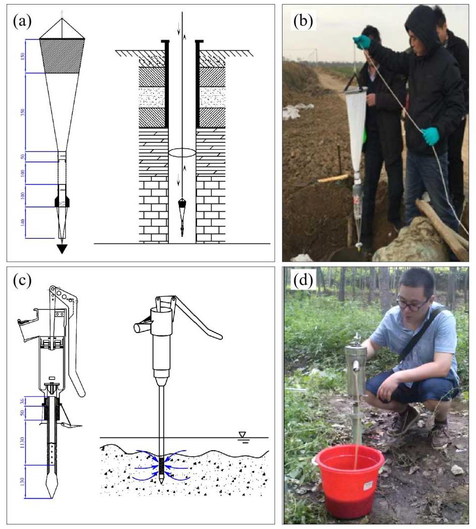
Figure 4 The structure and use of two stygofauna samplers: (a, b) phreatobiological net sampling and (c, d) micro-pump sampling.

Benthic invertebrates were kept in 70 % ethanol or 5 % formalin, Zooplankton (Cladocerans, Copepods) were saved in 100 mL water samples with 4 to 5 mL formalin, Zooplankton (Protozoa, Rotifers) were saved in water samples with 1 % ($v/v$) Lugol's solution, and fishes were stored with 10 % formalin. The morphological characteristics of the stygofauna were observed by a stereoscopic biological microscope (Olympus SZ61).

2.5 Data

In this paper, the data mainly include remote sensing data and hydrogeological survey data (Table 1). The remote sensing data used are the Landsat series of satellite datasets, Landsat collection 2, the second major reprocessing effort of the Landsat archive, which resulted in several data product improvements through the application of advancements in data processing and algorithm development. These images contain five visible and near-infrared (VNIR) bands and two short-wave infrared (SWIR) bands processed to orthorectified surface reflectance and one thermal infrared (TIR) band processed to orthorectified surface temperature (Cook et al., 2014). We use Google Earth Engine (GEE) to handle and calculate remote sensing data, mainly including image merging, cropping, and cloud removal, etc. According to the precipitation in the study area, we selected the dry season and rainy season from December 2020 to March 2021 and from April to October 2021, respectively. Correspondingly, the time of our field investigation is consistent with the time of remote sensing imaging.

The elevation data used are the Shuttle Radar Topography Mission (SRTM; see Farr et al., 2007) digital elevation data, an international research effort that obtained digital elevation models on a near-global scale, and the grid slope is calculated from the digital elevation. This SRTM V3 product (SRTM Plus) is provided by National Aeronautics and Space Administration Jet Propulsion Laboratory (NASA JPL) at a resolution of 1 arcsec (approximately 30 m).

The field survey mainly includes hydrogeological survey and GIS data preparation. The surface geological lithology of the LRB is extracted from the Chinese stratigraphic lithology dataset (1 : 2 500 000), which mainly includes geological lithology, geological body boundaries, amphibole schists, crater points, and other elements. Furthermore, we measured the riverbed levels and groundwater levels of the Quaternary aquifer and carbonate aquifer along the Langxi River, and the measurement locations are shown in Fig. 1, and the time series of the average groundwater level in the LRB are shown in Fig. S1. The maximum root depth of the watershed vegetation was drawn based on the effective soil depth and effective soil volume related to the presence of gravel and stoniness in the Harmonized World Soil Database and field surveys. Based on the measured groundwater level contour and the water level of the Langxi River, we can draw the surplus and deficit reaches where the groundwater recharges the river. Combined with the DEM topographic map, the groundwater confined artesian area can be divided, and the groundwater level in this area can be used to determine the GDE distribution area with shallow groundwater. In addition, water hydrochemical and groundwater fauna sampling also belong to field surveys; see the verifying part of GDEs (Sect. 3.3) for details.

3 Results

3.1 Hydrogeological investigation of three types of GDEs

3.1.1 Hydrogeological survey for S-GDE and V-GDE

The research acquired information about the maximum vegetation root depth, river bottom elevation, and groundwater level of the LRB (Fig. 5a) by the gathering of GIS data and basin hydrogeological surveys. We qualitatively evaluated the gain and loss of river portions using data on the elevation of the riverbed and the depth of the groundwater table (Fig. 5b).

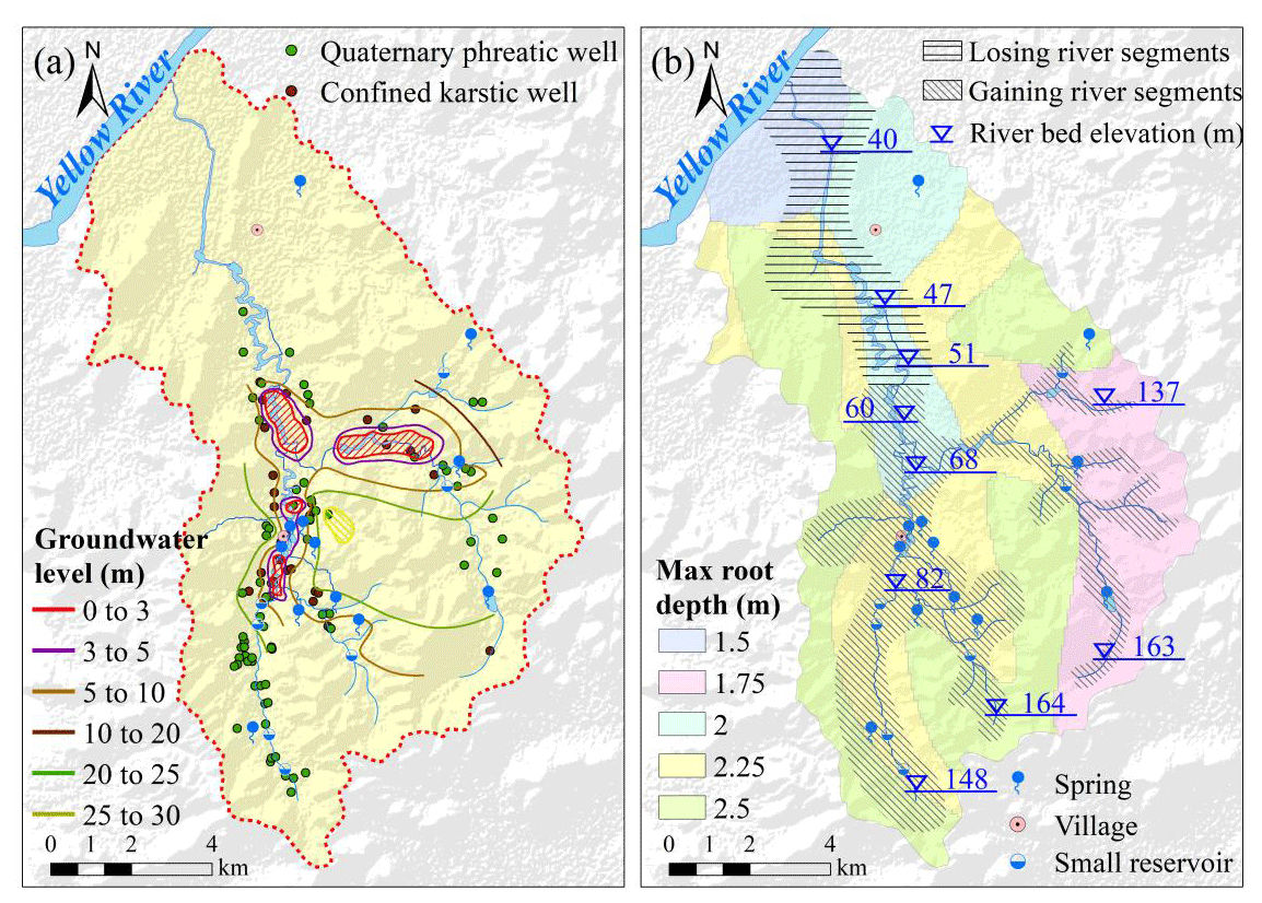
Figure 5 Summary of hydrogeological survey data in the LRB. (a) Distribution map of groundwater level, (b) maximum vegetation root depth, riverbed elevation, and water gain and loss in the river segments.

The analysis of underground water table depths reveals that the shallow water table area (0 to 5 m) is primarily located in the middle of the basin where the tributaries converge, and numerous karst springs are situated nearby. The vegetation in the LRB is predominantly composed of deciduous broad-leaved forest and deciduous open shrubs, with relatively developed underground root systems owing to the year-round flow of rivers. The maximum root depth in the basin ranges from 1.5 to 2.5 m, with some depths exceeding 4.5 m. Areas with deeper root depths are present on both sides of the river. In the lower reaches of the Langxi River near the Yellow River, the roots of vegetation are relatively shallow, consistently with the spatial distribution of surface lithology. However, the reason for the shallow roots is not caused by the surface lithology. Rather, they result from the abundant water supply in the area and the extensive distribution of farmland within this region. The riverbed bottom level changes more gently from upstream to downstream compared to the change in elevation. Based on the identification of potential GDEs, the study was able to accurately divide S-GDEs and V-GDEs.

3.1.2 Karst springs and K-GDEs

Based on historical data and hydrogeological survey results, the springs in the basin are mainly composed of ascending springs, depression springs, sinkholes, groundwater seeps, and artificial artesian wells. Table 2 displays the location, type of spring, flow rate, and other relevant information regarding the karst springs in the basin.

Table 2 Summary of karst spring field investigation in the Langxi River basin (LRB).

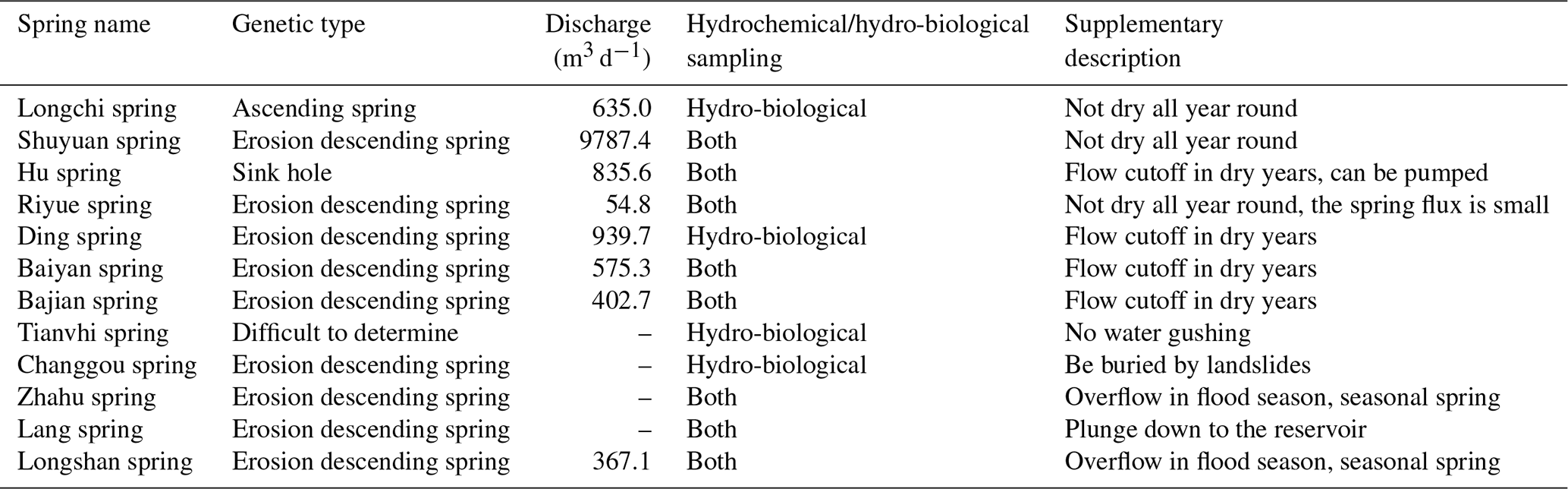
In the Hongfanchi Town area, the majority of the Zhangxia Formation aquifers are exposed on the surface, with the buried limestone ranging from 5 to 60 m from south to north. Underlying the rock strata is a purple shale and mudstone of the Mantou Group, which acts as a superior water-resisting layer compared to Zhangxia Group aquifers in other regions. The bottom of the Zhangxia Group limestone, along the karstic fissures, is where tectonic development occurs and is mainly exposed in the form of depression or descending springs, such as the Shuyuan spring, Ding spring, and Bajian spring, among others. Among these springs, Shuyuan spring has the highest daily spring discharge of over 9700 m³ d⁻¹.

Along the left bank of the Langxi River, some springs, such as Longchi and the artesian wells, belong to the ascending-spring category. Longchi spring water is pressurized in the confined karst aquifer, flowing upward, and gushes out with an average discharge of 635 m³ d⁻¹ through the thin Quaternary strata, which consists of pebbles mixed with sandy clays.

Another significant spring in the basin is Huquan spring, which belongs to the sinkhole and has an average discharge of 835.6 m³ d⁻¹. It exposes a large amount of water to the surface, especially during periods of abundant rainfall. The basin also contains other karst springs and groundwater seeps that are scattered throughout the area. Some of these springs flow seasonally, while others have ceased flowing altogether. Additionally, some of these springs have emerged as a result of water engineering construction and groundwater extraction.

3.2 Distribution and mapping of GDEs

3.2.1 Distribution of potential GDEs

Based on the research framework in Fig. 3, the study first uses remote sensing indicators such as terrain, NDVI, NDWI, and DWN to identify characteristics such as waters, bare land, wetlands, and vegetation to determine the potential distribution of GDE. Figure S2 displays the distribution characteristics of NDVI and NDWI in the study area at the end of the dry and wet seasons. In the central and southern plains of the study area, NDVI remained high at the end of the wet season (Fig. S2a) and decreased slightly at the end of the dry season (Fig. S2b), indicating that the vegetation in this area primarily experiences rapid drying. In the northern part of the study area, adjacent to the Yellow River, where numerous crops are cultivated, the NDVI value at the end of the dry season ranged between 0.2 and 0.3, which is slightly higher than the average value of 0.1 (Fig. S2b). It is noteworthy that, unlike in other similar studies, the NDWI did not exhibit significant differentiation at the two time points. The NDWI in the southern mountainous area and the northern planting area ranged between 0.3 and 0.4 at the end of the wet season, while, in other areas, it ranged between 0 and 0.2 (Fig. S2c). At the end of the dry season, the overall NDWI in the study area improved, but the spatial distinction was even less obvious (Fig. S2d).

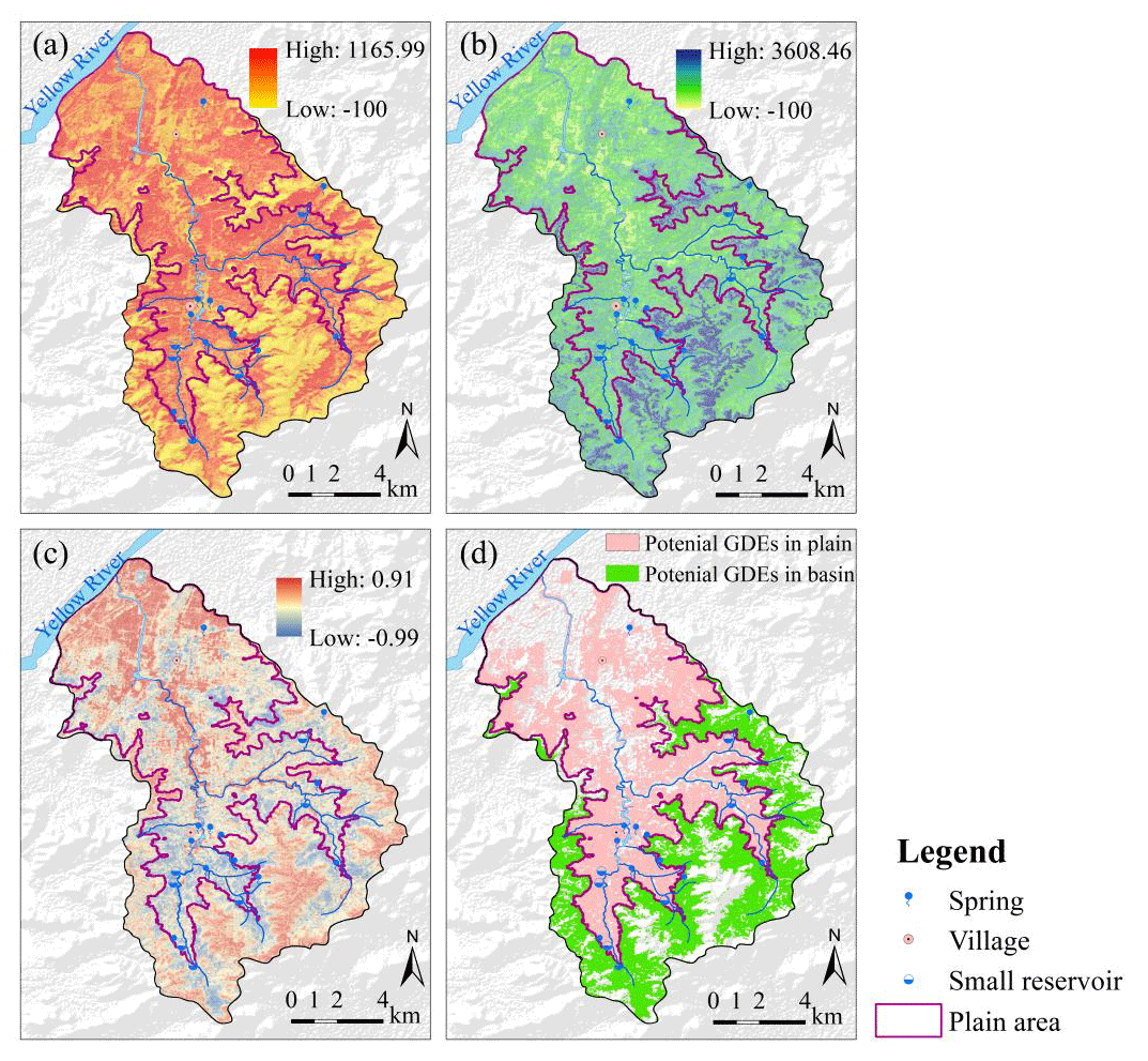
Figure 6 Change rate (%) of WET (a) and NDBSI (b) between wet and dry seasons in 2020 to 2021, (c) the mean difference (−) between WET and NDBSI, and (d) the potential GDEs in the plain area and basin using remote sensing data. NDBSI: the normalized difference built up and the soil index.

Figure 6a and b illustrate the change rates of WET and NDBSI in the wet and dry seasons between 2020 and 2021. The purple boundary line in the figure represents the shallow underground level identified by the GDE distribution area identification method. The WET index shows a higher change rate in the plain area compared to in the hilly area, where the humidity does not change much. The plain area near the boundary between the hills and the plain experiences a significant change rate in the WET index. Conversely, changes in the WET index are relatively small along the river banks and in the northern part of the lower-lying basin (Fig. 6a). In contrast to the WET index, the NDBSI changes relatively insignificantly in the plain area but exhibits larger changes in the ridges of the basin runoff area (Fig. 6b).

The average difference between WET and NDBSI during the dry and wet seasons indicates the variation in water availability between the two seasons with different amounts of water (Fig. 6c). High differences in certain areas suggest the availability of relatively stable water supply during the dry season. Analysis of lithology and water sources in the basin reveals that karst groundwater supply is the major source of stable water supply in these areas. Equation (7) is used to estimate the potential distribution range of GDEs based on remote sensing images during the dry and wet seasons of the same year, as depicted in Fig. 6d. The potential GDE range identified from the overlay map of the dry season reveals that, although the hilly area has abundant vegetation, the soil moisture is poor (Fig. 6a and b), and, thus, these areas may not be considered to be potential GDE distribution areas (Fig. 6d green area). However, the variation trends of WET and NDBSI indices can be well distinguished in the plain area, which is the boundary between the mountainous and non-mountainous regions. As a result, we can extract potential GDE areas with better soil moisture stability throughout the year (Fig. 6d, pink area). The distribution area of potential GDEs is relatively extensive, covering the upper and lower reaches of rivers, as well as some vegetation areas in hilly plains. Nevertheless, further hydrogeological investigations are required to determine if these areas can receive groundwater recharge.

The charts in Fig. 7 demonstrate that the difference index,the NDVI, and the centroid scatter of NDWI can effectively distinguish between vegetation within and outside the potential GDE range. Furthermore, the permanent waterbody in the area remains relatively consistent between the dry and wet seasons, aligning closely with the 1:1 line. The discernment between vegetation and water is highly accurate, with the slow-drying vegetation exhibiting a difference index range of −0.4 to 0 at the end of the wet season and of 0 to 0.4 at the end of the dry season. The difference index of fast-drying vegetation in the plain area ranges from 0.4 to 0.8 at the end of the wet season and from −0.4 to 0 at the end of the dry season. In contrast, the difference index between fast-drying vegetation and crops in mountainous areas is in the range of 0.4 to 0.8 at the end of the wet season and in the range of 0.6 to 1 at the end of the dry season. It is noteworthy that, compared with crops, the same difference index at the end of the wet season is smaller for the fast-drying vegetation in mountainous areas at the end of the dry season, indicating a smaller regression coefficient between the two (Fig. 7a).

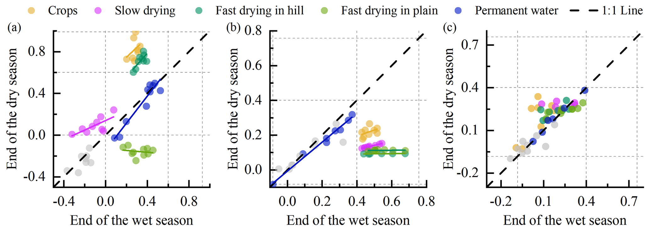
Figure 7 The centroid scatterplots for the difference between WET and NDBSI (a), NDVI (b), and NDWI (c) at the end of the wet season and the dry season (2020 to 2021).

Numerous studies define the NDVI range of 0 to 0.4 as the area covered by sparse vegetation, while areas with NDVI values greater than 0.4 are considered to be the area covered by vegetation. The most significant difference is observed between the NDVI values of crops during the wet and dry seasons and the vegetation in the basin. The NDVI of slow-drying vegetation at the end of the dry season is higher than that of fast-drying vegetation, and its regression coefficients at the end of the wet and dry seasons are also greater than those of fast-drying vegetation (Fig. 7b). These findings are consistent with the research by Barron et al. (2014) on distinguishing between slow-drying and fast-drying vegetation in western Australia. Compared to the previous two indices, NDWI is not effective in distinguishing the range of vegetation, including GDEs, due to various factors such as geographical location and climate (Fig. 7c). This indicates that the selected remote sensing index in the study has a relatively strong feasibility.

3.2.2 Distribution of GDEs in the LRB

Based on the previous ecological and hydrogeological survey results, the study subdivided potential GDEs into S-GDEs, V-GDEs, and K-GDEs according to the four-diagnostic-criteria framework (Fig. 3) and used the spatial kernel density function for mapping. The distribution results of GDEs in the basin are shown in Fig. 8. Green, orange, and magenta represent V-GDEs, K-GDEs, and S-GDEs, respectively. The depth of the color represents the spatial core density of the GDE. When the climate is dry, areas with lower spatial core density will gradually no longer belong to the scope of the GDE. The GDEs in the basin are mainly located in the central and western parts of the LRB, covering an area of approximately 49 km², which accounts for 29 % of the basin's total area. Although the river runs through the karst area, the spatial distribution of its center is not consistent with the surface-water-enriched river course and small reservoirs, which is a notable characteristic of GDEs identified in this study. The surface water in the karst region recharges the groundwater through lateral discharge, but this recharge is not concentrated on the river channel; instead, both sides of the river channel are equally affected. Therefore, the shape of GDEs reflects the trend of underground aquifers on the ground, which is in agreement with the GDE definition and distribution results reported by Erostate et al. (2020) and Duran-Llacer et al. (2022). We divided the coverage of GDEs into four levels based on the kernel density gradient histogram, which aligns better with the actual distribution under different water recharge conditions.

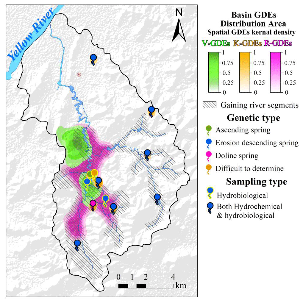
Figure 8 Langxi River basin GDE distribution area.

The results depicted in Fig. 8 indicate that the distribution of GDEs is significantly impacted by human activities, not only in the surface water system but also in the groundwater system, including aquifers. It is evident that the GDEs in the northern and eastern regions terminate at the dam, indicating that water conservancy facilities situated on the main channel of the Langxi River obstruct and disrupt the connectivity of surface and underground water.

3.3 Ecohydrological signals of GDEs

3.3.1 Base flow

The Shuyuan spring and Langxi River profile (hereinafter referred to as the Shuyuan spring profile, Fig. 2) show the location and elevation relationship between groundwater and the Langxi River profile. The eastern Cambrian Zhushadong–Zhangxia Formation limestone is rich in groundwater buried deeper than the river. Shuyuan spring, one of the descending springs in the basin, gushes out at the intersection of the Quaternary sedimentary layer and the Cambrian Zhushadong–Zhangxia Formation limestone. At the same time, groundwater also recharges to the Langxi River along the stratigraphic fissures. Based on the hydrogeological graph spanning from 1990 to 2015 (Fig. 9), it is evident that the river flow near the Shuyuan spring section is highly dependent on precipitation. The maximum discharge recorded was 1450 L s⁻¹ in 2004, while the minimum average discharge was 6.87 L s⁻¹ in 2015, which is more than 211 times lower than the maximum value (Fig. 9a). The average annual discharge and daily discharge are 89.66 L s⁻¹ and 7746 m³, respectively. Despite this variation in flow, the base flow is maintained even during dry seasons, with the base flow index (BFI) accounting for 54.15 % of the river flow. Among them, the minimum BFI was 0.369 in 1991, and the maximum was 0.845 in 2013. It can be seen that the base flow has always made a large contribution to the runoff of the basin. Even in the long period of recharge, the base flow presents a decay trend and lasts for a long time until the next rainfall. Therefore, we chose July 1993 to July 1994 as a typical year to analyze the change process of precipitation and Shuyuan section discharge to illustrate how groundwater and springs feed the river. It can be seen that there were two obvious flow decline processes in this year (Fig. 9b). Among them, there was almost no precipitation between November 1993 and April 1994, indicating that the river flow was mainly influenced by groundwater and spring discharge.

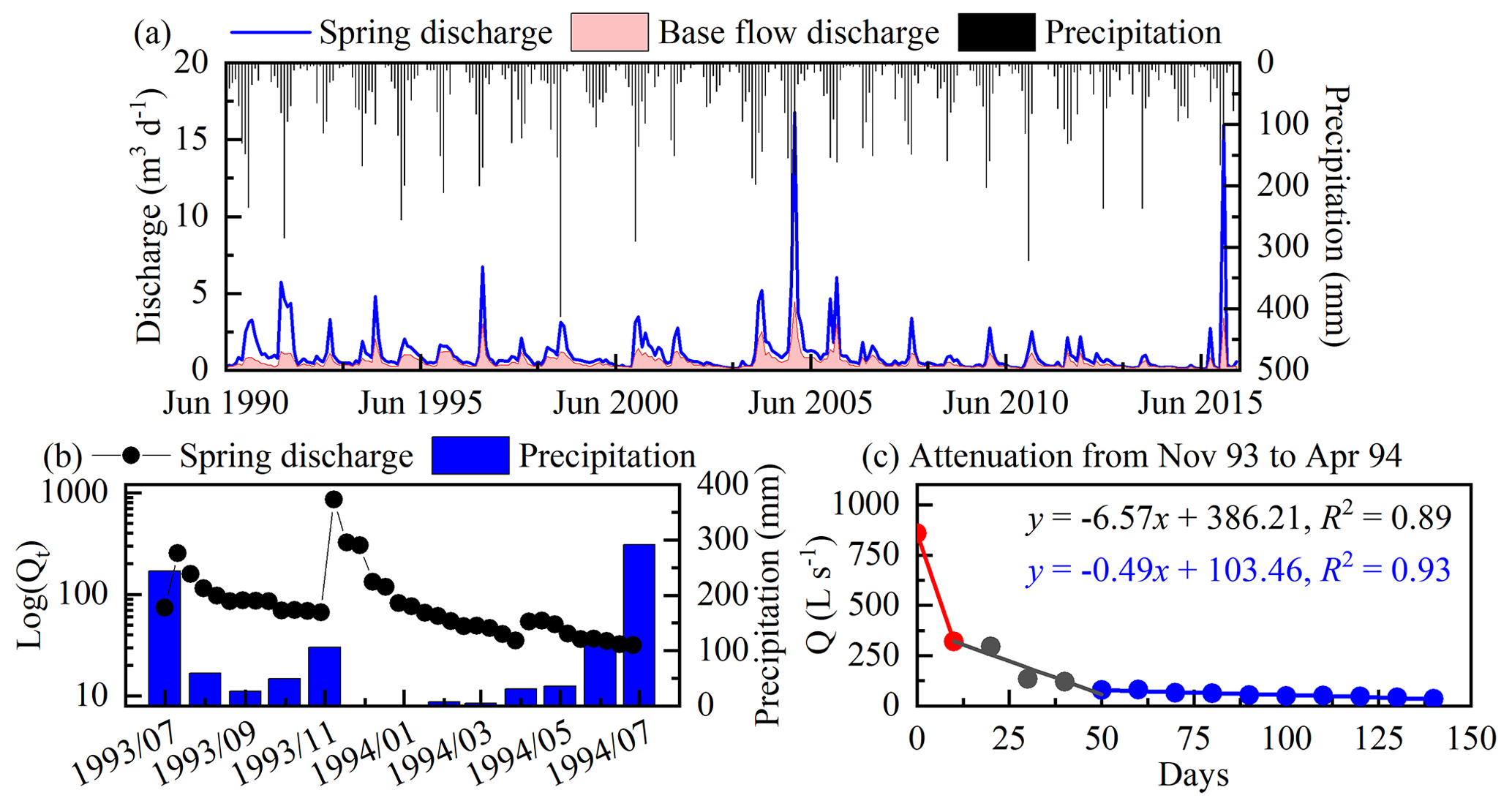
Figure 9 (a) Relationship between precipitation and Shuyuan section river flow and its base flow from 1990 to 2015, (b) hydrologic graph of Shuyuan spring from July 1993 to July 1994, and (c) spring discharge attenuation curve of Shuyuan spring from November 1993 to April 1994.

We selected the hydrological graph from November 1993 to April 1994 (Fig. 10c) for a period with no precipitation and groundwater exploitation. It was found that the rivers during this no-rain-recharge period were mainly sustained by spring water, and the flow rate showed an exponential decay trend. The flow attenuation presents three stages, which we believe are represented by the red-line segment, indicating the concentrated flow with turbulence in the karst conduit to recharge the river; the black line, indicating the large corrosion voids and fractures supplying fracture flow; and the blue lines, indicating the small corrosion cracks, fractures, and intergranular pores recharging the diffuse-flow aquifer with diffuse flows and laminarity.

Upon comparing the attenuation coefficient (α) of different stages, it is evident that the attenuation coefficient of the first sub-dynamic stage (0 to 10 d) is the largest at 0.0985. The attenuation coefficient of the second sub-dynamic stage (10 to 51 d) is significantly weakened, while the attenuation coefficient of the third sub-dynamic stage (51 to 141 d) gradually approaches 0. From the above analysis, it is evident that, even during a prolonged period of no rain recharge, the flow attenuation can be sustained for an extended period, indicating that groundwater has consistently contributed to the Langxi River's flow.

3.3.2 Hydrochemical types

In this paper, 10 water samples, including karst groundwater, Quaternary pore water, and surface water, were collected and tested in the laboratory. The results were then plotted onto a piper plot, as shown in Fig. 10a. The chemical indicators of the water, such as DO, pH, EC, and total dissolved solids (TDSs), were analyzed and clustered to create a diagram, which is presented in Fig. 10b.

Figure 10 Hydrochemical characteristics of 10 water samples in the LRB.

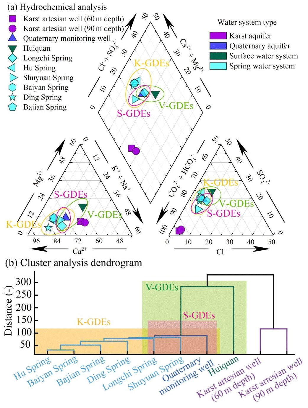
Based on the hydrochemical analysis, most of the water samples had a pH value in the range of 7 to 7.5, indicating a weakly alkaline environment. The hydrochemical type of the limestone aquifer water samples in the monitoring well was mainly HCO₃–Ca⋅Na, while the other water samples were of the HCO₃–Ca type. From the piper plot and the cluster diagram, the data can be divided into three clustering groups. The first clustering group consists of groundwater with depths ranging from 60 to 90 m in the monitoring well, reflecting the groundwater characteristics of the Cambrian Zhangxia Group karst confined aquifer. The second clustering group includes water from Longchi spring, Hu spring, Shuyuan spring, Ding spring, and Bajian spring, which are mainly natural outcrops of groundwater, reflecting the characteristics of karst spring water. The third clustering group consists of the Quaternary pore water and water from the Huiquan Reservoir, reflecting the reservoir mainly replenished by shallow groundwater.

Combined with the distribution range of the three GDEs and the water sample collection locations in Fig. 8, we can clearly see that the hydrochemical characteristics of waterbodies of the same GDE type have obvious clustering relationships. The overlapping relationship of hydrochemical characteristics in GDE groups is consistent with the distribution characteristics of GDE types at the spatial scale of the basin (Fig. 10a), which is also reflected in the cluster analysis diagram (Fig. 10b). In addition, descending springs like Shuyuan spring are not only closely related to karst aquifers but also have good hydraulic connections with Quaternary aquifers. On the other hand, Huiquan Reservoir is a surface reservoir stored in a river barrage and receives a large amount of groundwater recharge. Therefore, it exhibits hydrochemical characteristics similar to spring water and Quaternary pore water. It can be seen that the interaction between surface water and groundwater in this area is strong, and there are obvious differences in the hydrochemical characteristics of GDE, but there are also certain similarities.

3.3.3 Groundwater fauna species

Samples of groundwater fauna were collected from various types of GDEs, including karst cave (sink hole), karst aquifer, depression spring, ascending spring, and river hyporheic zone. Based on laboratory identification, the primary stygofauna found in these GDEs were Neocaridina denticulata sinensis, chironomid larvae, Pentaneura sp., Dytiscidae, Radix lagotis, Gyraulus, and Galba pervia (Table 4).

Table 3 Summary of groundwater fauna sampling of the GDEs.

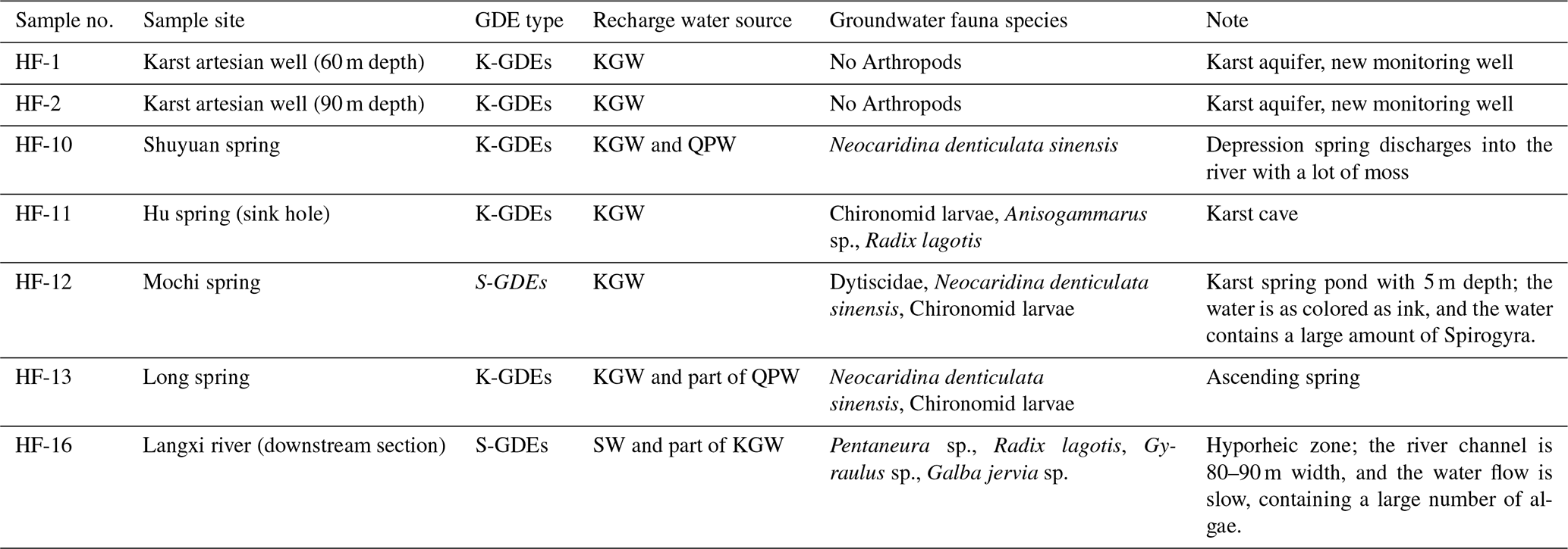
Note: K-GDEs and S-GDEs are karst-type GDEs and stream-type GDEs; KGW, QPW, and SW are karst groundwater, Quaternary pore water, and surface water.

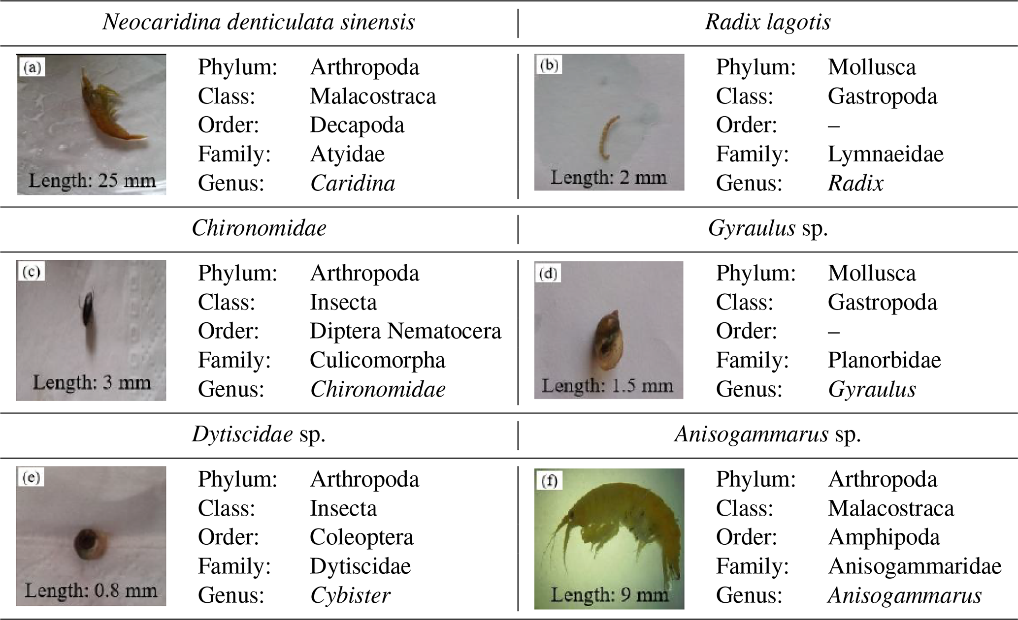
Table 4 Groundwater fauna samples. (a) Neocaridina denticulata sinensis, (b) Radix lagotis, (c) Chironomidae, (d) Gyraulus sp.; (e) Dytiscidae sp., (f) Anisogammarus sp.

Finding groundwater fauna near karst caves is easy because there is an abundance of food, making it easier for them to survive. Hu spring, a natural karst cave, is home to three species of Chironomid larvae, and Anisogammarus sp. and Radix lagotis were found in it. Typically, these faunas mainly comprise of arthropods, coelenterates, and mollusks that live in groundwater throughout their entire life cycle, and are known as stygobites, a true groundwater fauna. Combining the spatial distribution range of GDEs in Fig. 8 of this study and the groundwater fauna in Tables 3 and 4, it can be seen that these groundwater fauna appear not only in the range of K-GDEs with caves and karst springs but also in the range of some S-GDEs and a small number of V-GDEs.

As groundwater levels deepen, there are fewer aquatic organisms present. Hahn and Matzke (2005) discovered that the screen of an artificial borehole would not prevent groundwater organisms from passing through, but we did not observe any organisms in the two new monitoring wells. Many species of groundwater fauna, including Neocaridina denticulata sinensis, Chironomidae larvae, and Dytiscidae, were found in the sink pool of depression and ascending springs. Neocaridina denticulata sinensis, also known as Penaeus monodon, is a flagship species among the many aquatic organisms found in the sink pool. It has a dark-green body and is a very small shrimp, measuring only 5 to 10 mm in length. It primarily inhabits freshwater ponds with abundant aquatic plants and has the highest yield in autumn. There are also many species distributed throughout the river hyporheic zone. The river hyporheic zone also harbors a variety of species. Dytiscidae, also known as terrapin or aquatic beetles, are a type of arthropod that range from 3 to 5 mm in length, with varying individual sizes. The adults have a long streamlined body, flat and smooth with an arched back, and developed bristles. Radix lagotis, a type of aquatic snail, is about 1.5 mm long and has a thin, slightly hard shell with an elliptical shape. It is found in the wild. Gyraulus, another type of aquatic snail, measures about 8 mm in length. Galba pervia, a species of freshwater snail, is about 4 mm long and can be found in various still waters and slow-flowing waters. These species are representative of benthic types of groundwater fauna. Chironomidae is a widely distributed species among groundwater fauna, with Chironomid larvae being found, in particular, in waterbodies that have good-quality and highly dissolved oxygen (DO) content. This species belongs to the stygophilies, which are a type of groundwater fauna.

In summary, various types of GDEs such as karst caves, karst aquifers, karst springs, and river hyporheic zones host distinct populations of groundwater fauna and iconic species. This information can be used to confirm the distribution of GDEs.

4 Discussion

4.1 Four-diagnostic-criteria framework

The aim of the framework presented in this paper is to offer a comprehensive methodology, rather than a specific method, for identifying and evaluating GDEs. This methodology not only incorporates existing approaches for identifying GDEs but also applies to basins with varying climatic and geological conditions. For instance, the surface vegetation type can be more accurately identified using NDVI and NDWI in Barron et al. (2014)'s study, whereas, in our framework, it is advisable to experiment with multiple indices. The outcomes shown in Fig. 6 additionally confirm the viability of using remote sensing indices to identify potential GDEs, as well as the unsuitability of NDWI in the LRB.

Compared with the study of El-Hokayem et al. (2023) on identifying GDEs in Italy, this study did not include climate factors in the identification indicators. Instead, it focused more on elements of the local watershed itself, such as waterbody characteristics and groundwater biological characteristics. This is because the study area of El-Hokayem et al. (2023) belongs to the coastal area, and the vegetation responds more sensitively to climate elements. Our research prefers to identify and establish direct connections between groundwater–surface water–surface or near-surface ecosystems through hydrochemical characteristics and then to verify the identification scope of GDEs.

The research results of Duran-Llacer et al. (2022) using more than 10 terrain and remote sensing indicators to identify and map GDEs in Chile showed that increasing the input variables of the identification model can help improve the accuracy of identification. This can be used as a reference for the application of the identification framework proposed in this study to other basins. The multi-index verification system of hydrological rhythm, water chemistry, and groundwater fauna used in this study can verify the accuracy of GDE identification in multiple dimensions, which has basically not been used in existing research. Furthermore, this will help provide stronger support for the results for verification in future relevant studies.

The kernel density function chosen to be used in our framework is to expand the areal scale by using the probability density for the uncertain groundwater recharge range (Pérez Hoyos et al., 2016). The advantage of this is that the GDE area can be quickly identified using simple survey data under conditions determined by factors such as topography and remote sensing (Doody et al., 2017; Paz et al., 2017). It is important to acknowledge that the methodology for identifying GDEs still faces limitations, particularly in the precise definition of the scope of influence of fine-grained GDEs (Martínez-Santos et al., 2021), such as K-GDEs. This challenge remains unresolved in the field. Even for S-GDEs and V-GDEs, determining their scope requires extensive on-site investigation and hydrogeological, groundwater, and vegetation data (Erostate et al., 2020). Furthermore, these data must be relatively time-sensitive, as per existing research.

The quantity and range of groundwater recharge will affect the GDEs' distribution ranges. The effects of climate change and human activity will gradually alter the volume and scope of groundwater recharge. The distribution range of GDEs can be altered dramatically in a short amount of time when major changes are made to subterranean aquifers by natural disasters like earthquakes, coal mining, or human activity. It should be noted that, when the groundwater level fluctuates significantly or when the stratigraphy changes significantly, we recommend re-evaluating the relevant indices and parameters in the study area and this system. Long-term groundwater level monitoring data indicate that the changes in groundwater levels in the entirety of the LRB and in its vicinity are very weak during the period when the stratum does not change significantly. Therefore, the four-diagnostic-criteria framework proposed in the study can effectively identify GDEs in areas such as grasslands, deserts, plains, and karsts in arid, semi-arid, and sub-humid areas.

4.2 Groundwater connectivity should be focused

The four diagnostic criteria proposed in the study that combines GIS and hydrogeological surveys are valuable for the identification and mapping of GDEs. However, remote sensing methods can only identify potential distribution areas of GDEs, and they are not sufficient for accurately describing the actual distribution of GDEs. For instance, we need to determine when and how much groundwater replenishes GDEs, as well as the extent to which the roots of various vegetation communities can absorb groundwater. These groundwater connectivity processes necessitate careful hydrogeological investigation, particularly through the use of hydrogen and oxygen isotope tracing methods. Given that identifying GDEs is a fundamental issue, some authors have also examined the impact of groundwater extraction and other factors (Gou et al., 2015; Münch and Conrad, 2007; Pérez Hoyos et al., 2016). We think that future studies can quantitatively link groundwater and ecosystems through the use of stable hydrogen and oxygen isotope experimental data regarding vegetation's absorption of groundwater in conjunction with ecological or ecohydrological models.

4.3 Groundwater fauna tracing would be necessary

The relative spatial independence of groundwater fauna in karst spring-type GDEs can serve as an indicator for identifying such systems. However, sampling stygofauna poses a greater challenge due to the complex trajectories of groundwater fauna, including species fluctuations observed in sink holes, as well as limitations in sampling and tracing methods. Various methods are currently used for sampling stygofauna, each with its own advantages and disadvantages (Hahn, 2002; Leijs et al., 2009; Smith et al., 2016). Nevertheless, there are currently no standardized methods for sampling stygofauna (Hahn and Matzke, 2005). Net sampling is the most efficient and cost-effective method for quickly obtaining numerous stygofauna samples. However, using a mesh size of 74 or even 40 µm makes it challenging to collect all sample types, particularly during dry seasons. Water sampling, which involves pumping with a homemade bio-pump and filtering with a 74 µm filter, is another swift and economical option, but the pumped water volume is limited. In some cases, columnar species were not discovered due to screening barriers, making it challenging to track groundwater fauna. To address this, real-time monitoring, tracing, and DNA-sequencing technologies can extract essential genetic markers of groundwater fauna, facilitating the study of biotic connectivity between groundwater and GDEs. This could be a significant breakthrough in groundwater fauna research.

4.4 Impacts of human activities and climate change should be of more concern

GDEs have always been impacted by climatic variations, but with the increasing scale of human activities, new stresses are emerging. It is essential to focus on the hydrological and ecosystem response to these stresses. To better understand the vulnerability of GDEs, regional studies are necessary. It is crucial to comprehend the role of human activities and climate change to identify potential human impacts and to put climate change trends into perspective (Barron et al., 2012; Gurdak et al., 2007; Kløve et al., 2014; Liu et al., 2016; Randhir and Hawes, 2009). Karst groundwater ecosystems are generally more vulnerable than other ecosystems due to the specific features of the karst zone, such as high permeability and rapid infiltration or recharge rates and being mainly controlled by karst conduits. Therefore, it is essential to monitor changes in the static water level, groundwater discharge to streams, and riparian plants resulting from changes in precipitation, runoff, and water use. Additionally, we must determine if land consolidation, engineering construction, and other human activities are disrupting the groundwater up-flowing or recharging route. To fully comprehend these complex factors and interactions, further studies are necessary (Kløve et al., 2011).

5 Conclusion

This paper proposes a framework of four diagnostic criteria that combines remote sensing, GIS data, and field hydrogeological surveys. This framework can effectively identify and map different types of GDEs in a typical karst basin. Compared to the traditional NDVI and NDWI index division, the difference index of WET and NDBSI has better adaptability for identifying potential GDE distributions. The GDEs are then mapped using spatial kernel density functions. The results reveal that there are three main types of GDEs. River-type and vegetation-type GDEs are concentrated along the Langxi River riparian zone, while karst-aquifer-type GDEs are scattered throughout the basin. Each type of GDE displays special ecohydrological signals. For instance, one of the obvious signals for the gaining stream is the base flow index, which can reach about 54.15 %, keeping the river flowing even during extremely dry seasons. The second signal is the clustering of hydrochemical characteristic ions, which reveals whether the GDEs are replenished by karst groundwater or other water sources. The third unique ecohydrological signal is the groundwater fauna that live in different types of GDEs. These three signals can be utilized to evaluate the accuracy of identifying and mapping GDEs. However, the knowledge gap regarding the ecohydrological connectivity between groundwater and GDE can be improved by utilizing isotope analysis, stygofauna tracing, and DNA-sequencing technology under the recommended four-diagnostic-criteria framework in the future. The research helps to better understand the connection between groundwater and ecosystems, and the results can guide decision-makers in groundwater exploitation in karst areas.