the Creative Commons Attribution 4.0 License.
the Creative Commons Attribution 4.0 License.
 | 07 Feb 2024
The application and modification of WRF-Hydro/Glacier to a cold-based Antarctic glacier
Tamara Pletzer
Jonathan P. Conway
Nicolas J. Cullen
Trude Eidhammer
Marwan Katurji
The McMurdo Dry Valleys (MDV) are home to a unique microbial ecosystem that is dependent on the availability of freshwater. This is a polar desert and freshwater originates almost entirely from surface and near-surface melt of the cold-based glaciers. Understanding the future evolution of these environments requires the simulation of the full chain of physical processes from net radiative forcing, surface energy balance, melt, runoff and transport of meltwater in stream channels from the glaciers to the terminal lakes where the microbial community resides. To establish a new framework to do this, we present the first application of WRF-Hydro/Glacier in the MDV, which as a fully distributed hydrological model has the capability to resolve the streams from the glaciers to the bare land that surround them. Given that meltwater generation in the MDV is almost entirely dependent on small changes in the energy balance of the glaciers, the aim of this study is to optimize the multi-layer snowpack scheme that is embedded in WRF-Hydro/Glacier to ensure that the feedbacks between albedo, snowfall and melt are fully resolved. To achieve this, WRF-Hydro/Glacier is implemented at a point scale using automatic weather station data on Commonwealth Glacier to physically model the onset, duration and end of melt over a 7-month period (1 August 2021 to 28 February 2022). To resolve the limited energetics controlling melt, it was necessary to (1) limit the percolation of meltwater through the ice layers in the multi-layer snowpack scheme and (2) optimize the parameters controlling the albedo of both snow and ice over the melt season based on observed spectral signatures of albedo. These modifications enabled the variability of broadband albedo over the melt season to be accurately simulated and ensured that modelled surface and near-surface temperatures, surface height change and runoff were fully resolved. By establishing a new framework that couples a detailed snowpack model to a fully distributed hydrological model, this work provides a stepping stone to model the spatial and temporal variability of melt and streamflow in the future, which will enable some of the unknown questions about the hydrological connectivity of the MDV to be answered.
- Article
(4747 KB) - Full-text XML
- BibTeX
- EndNote


Terrestrial Antarctic ecosystems exist almost entirely in ice-free regions. Under the highest emissions scenario, RCP 8.5, climate studies show that these ice-free regions may increase from 1 % of Antarctica to almost 25 % by the end of the century (Lee et al., 2017). Given the anticipated increase in ice-free regions in Antarctica, there is an urgent need to better understand the sensitivity of the McMurdo Dry Valleys (MDV) to climate variability and change. The MDV are currently the largest ice-free area in Antarctica and are home to a unique microbial ecosystem that resides in a system of streams and lakes situated on the valley floors. This ecosystem is dependent on freshwater that is sourced from glacial melt (Gooseff et al., 2011) for survival. It is expected that the biogeography of this ecosystem will be altered in response to the larger changes in climate impacting Antarctica, and thus it is key to understand and simulate how atmospheric warming will impact glacier melt and the hydrological connectivity of this unique environment.
Unlike most mid-latitude glaciers, the glaciers in the MDV are mainly cold-based, meaning that the subsurface temperatures are below the pressure melting point and ice is frozen to the bedrock (Fitzsimons, 1996; Gooseff et al., 2011; Fountain et al., 2016). MacDonell (2008) was the first to study the full hydrological drainage system and developed a conceptual modelling framework for cold-based glacial meltwater drainage processes on Lower Wright Glacier in Wright Valley. This study identified the need for a physically based, rather than empirical, model to simulate the complex drainage systems of MDV glaciers (MacDonell, 2008). Hoffman (2011) was the first to implement a distributed surface energy balance model and investigated the spatial and temporal distribution of mass and energy exchanges of several glaciers in Taylor Valley. This study showed that penetrating shortwave radiation and meltwater drainage are important for accurately modelling surface ablation on glaciers in the MDV (Hoffman, 2011). Cross et al. (2022) extended this work by coupling the glacier energy balance model used by Hoffman (2011) with a lake energy balance model to assess lake sublimation and the water budget. Whilst both Hoffman (2011) and Cross et al. (2022) model glacial runoff, neither explicitly models the off-glacier processes in the hydrological system, such as streams or soil moisture.
Similar to mid-latitude glaciers, glacial melt in the MDV is driven primarily by net radiation, which is sensitive to variability in solar radiation. What is different in the MDV is that energy and mass exchanges are often very small, with minor changes in the surface energetics capable of shifting the hydrological system from a frozen state to one that is melting. Thus, small changes in energy (e.g. through albedo) can have a very large impact on melt generation (Hoffman et al., 2008; Macdonell et al., 2013). It has also been observed that solar radiation penetrates the top 5–15 cm of the snow or ice surfaces on the glaciers in the MDV (Hoffman et al., 2014), and this near-surface layer can retain heat longer than the surface due to the solid-state greenhouse effect (Brandt and Warren, 1993). This effect extends the duration of melt events and model simulations suggest that melt from this layer can be an order of magnitude larger than surface melt (Hoffman et al., 2014). Despite solar radiation being crucial for modelling melt, no study has attempted to physically simulate the variability of albedo over the duration of a full melt season in the MDV. To ensure that the magnitude and duration of melt is captured sufficiently in a low-energy polar environment like the MDV, it is critical that glacier albedo is modelled accurately.
To resolve the hydrological connectivity in the MDV, it is necessary to identify the streams of meltwater from the glaciers to the bare land that surround them, including understanding how water is channelled into stream networks and stored in the numerous closed-basin lakes. The WRF-Hydro/Glacier modelling framework (Gochis et al., 2020; Eidhammer et al., 2021) provides an opportunity to physically model the hydrological cycle in the MDV due to its ability to resolve the connections between the atmosphere, glaciers, bare land, stream channels and lakes (the hydrological reservoirs). WRF-Hydro/Glacier contains a detailed snowpack model (Crocus), which is embedded in a distributed hydrological model (WRF-Hydro). Importantly, the model provides enough flexibility to be able to resolve the stream channels and streamflow from the glaciers to the surrounding landscape, which is critical given that the glaciers are the primary hydrologic reservoirs and are controlled by the daily, seasonal and annual cycles of the surface energy balance (Gooseff et al., 2011). Importantly, WRF-Hydro/Glacier can be applied at small catchment scales up to continental-scale domains, providing fully distributed hydrological modelling opportunities in the MDV and the larger surrounding regions. Eidhammer et al. (2021) implemented WRF-Hydro/Glacier on a temperate Norwegian glacier and demonstrated that the model was capable of simulating the mass balance, snow depth, surface albedo and runoff when compared to observations. However, the environmental setting of the cold-based MDV glaciers is vastly different from the temperate glaciers in Norway, with the dry polar climate of the MDV ensuring that summer melt generated from variability in the surface energy balance has a much stronger control on the hydrological cycle than precipitation (Gooseff et al., 2011).
Given the importance of the surface energy balance to meltwater generation, the modelling of albedo and near-surface melt on the MDV glaciers is critical. The detailed snowpack scheme in Crocus, which is embedded in WRF-Hydro/Glacier, has been implemented in a range of environments (Vionnet et al., 2012), including extremely cold (well below the melting point) conditions over the Antarctic ice sheet (such as Dome C) (Brun et al., 2011) and high-precipitation (both rain and snow) and relatively warm and melting conditions on temperate glaciers (Eidhammer et al., 2021). However, the challenge in implementing it on glaciers in the MDV is that the surface energy balance is more dominant than precipitation in governing variability in mass balance, largely through its influence on controlling melt and the associated feedbacks on surface albedo. The implication of this is that runoff and streamflow are entirely sourced from glacier melt rather than from precipitation (rainfall), as is common on temperate glaciers. In this context, the aim of this study is to optimize a multi-layer snowpack scheme (Crocus), which is embedded in WRF-Hydro/Glacier, to resolve the onset, duration and end of melt over a cold-based glacier in the MDV of Antarctica. If melt is sufficiently resolved in this modelling framework, it will allow the streams to the surrounding landscape (the other hydrological reservoirs) to be resolved at different spatial and temporal scales in future applications of WRF-Hydro/Glacier.
To achieve our primary aim, WRF-Hydro/Glacier is implemented at a point on Commonwealth Glacier in Taylor Valley, forced by automatic weather station data and tested against observations of broadband albedo, surface and near-surface ice temperatures, surface height change and streamflow. Given that this is the first time this modelling framework has been implemented in this unique environmental setting (cold-based glacier, energy balance dominates over precipitation, limited opportunities for the melting threshold to be reached), it was necessary to modify the percolation of water through the glacier and the spectral albedo scheme to accurately simulate the feedbacks between albedo, snowfall and melt. The limited energetics and complicated pathways for water transport in this environment make testing at a point scale using observational rather than modelled input data a critical first step towards modelling the full hydrological connectivity of glacial meltwater in the MDV.
The next section describes the WRF-Hydro/Glacier model set-up and initialization. Section 3 describes the site and the observational data used to force and validate the model. Section 4 details the modifications to the Crocus snowpack meltwater drainage and spectral albedo schemes necessary to adapt the model to the unique cold-based glacial environment of the MDV. Section 5 compares the performance of the original and modified versions of the model to observational data over the 2021/22 melt season, while Sect. 6 reflects on the significant advances made to WRF-Hydro/Glacier in this study and the platform it provides to resolve the full hydrological system in the MDV.
2.1 WRF-Hydro/Glacier
WRF-Hydro is a multi-scale and spatially distributed hydro-meteorological modelling system developed by NCAR (Gochis et al., 2020). The model links a column land surface model (Noah-MP) to subsurface flow, routing, overland flow, channel routing and water management modules (i.e. a reservoir). The model can be either forced by meteorological data or gridded atmospheric data. A schematic of the modelling system can be seen in Fig. 1. WRF-Hydro is currently the National Water Model in the contiguous USA. It has applications from flood forecasting to regional hydroclimate impact assessments and has been validated extensively across six continents (e.g. Senatore et al., 2015; Li et al., 2017; Xiang et al., 2017; Kerandi et al., 2018; Lahmers et al., 2021; Pal et al., 2021; Shafqat Mehboob et al., 2022). More recently, Eidhammer et al. (2021) developed the WRF-Hydro/Glacier model by embedding the detailed Crocus snowpack model in the Noah-MP land surface model in order to simulate the energy and mass balance over glacial surfaces. The snow module in Noah-MP does not allow the glacier to decrease in mass once the snow layers are melted because it represents the glacier as a bare ice land surface category with constant albedo, roughness length and heat conductivity. This representation does not allow melt and thus was not sufficient to model glacial melt and runoff (Eidhammer et al., 2021).
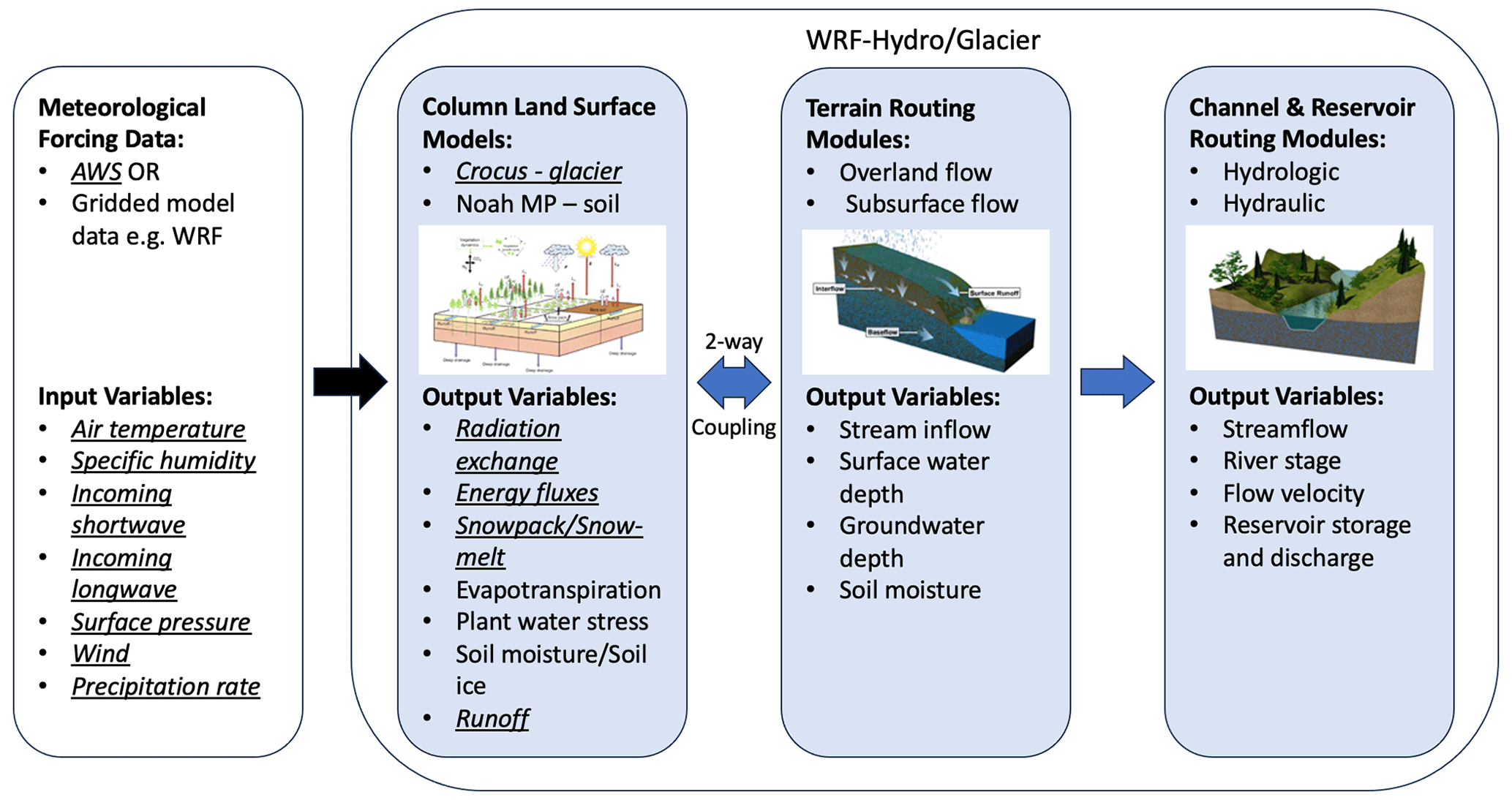
Figure 1Schematic of the WRF-Hydro/Glacier modelling framework. Modules and variables used in this study are displayed in italics and are underlined. Adapted from NCAR (https://ral.ucar.edu/sites/default/files/public/WRFHydroPhysicsComponentsandOutputVariables.png, last access: 8 August 2023).
Crocus is a detailed column snowpack model that was developed initially for avalanche forecasting in Col de Porte, France, by the Centre d'Etudes de la Neige of Météo-France (Brun et al., 1989, 1992). The model version implemented in WRF-Hydro/Glacier is described in Vionnet et al. (2012). This version was chosen by Eidhammer et al. (2021) due to extensive validation and its suitability for embedding in the Noah-MP land surface scheme. The model physics include schemes for snow metamorphism, compaction, albedo, penetrating solar radiation, energy balance fluxes, heat diffusion, melt, refreezing, percolation, runoff, sublimation and deposition. Crocus simulates state variables over a prescribed number of layers: heat content, thickness, density, age, history of snow and two snow grain properties that describe the dendricity, sphericity and grain size of the snow or ice crystals. All other variables such as snow temperature and liquid water content are calculated from the state variables. The number and thickness of vertical layers in Crocus change dynamically with time. Users define a maximum number of layers (n≥3), and when snowfall occurs, a new layer is added with a set of fresh snow characteristics. Over time, layers may merge with the layer below if the snow grain properties become the same. The layers at the top of the snowpack tend to be thinner to better solve the surface energy balance equation. Further information can be found in Vionnet et al. (2012) and Eidhammer et al. (2021).
3.1 Site description
Commonwealth Glacier is located on the eastern side of Taylor Valley approximately 4 km from McMurdo Sound (Fig. 2). It is a piedmont glacier, terminating in cliffs, and is characterized by a smooth surface. The mean annual temperature from 1986 to 2017 is −17.6 ∘C. However, in the summer temperatures can reach a maximum of 7.8 ∘C, and in winter the temperature can descend to a minimum of −45.0 ∘C (Obryk et al., 2020). The wind directions are characterized by a bimodal distribution in the summer, mainly a daytime easterly sea breeze coming from McMurdo Sound and a northerly down-glacier wind due to the low sun angle and the temperature differences between the glacier and bare land on the valley floor at nighttime (Fountain and Doran, 2004). In the winter, this down-glacier wind becomes more persistent as the ice cools more quickly than the bare land. There is also a low-frequency westerly in both summer and winter that is a down-valley wind (Nylen et al., 2004). The down-valley winds can either be a föhn wind generated by a synoptic cyclone or a katabatic wind descending from the Antarctic Plateau (Speirs et al., 2010; Steinhoff et al., 2013). Wind speeds on average are 2.2 m s−1, with the strongest ones reported reaching a maximum of 44.5 m s−1 (Obryk et al., 2020).
3.2 Automatic weather stations
Data from two automatic weather stations (AWSs) are used in this study. The CWG AWS was installed on 1 December 2021 and is used for tuning and validation. It is located at −77.56485, 163.2776∘ at 280 m elevation. CWG AWS measures air temperature, relative humidity, wind speed and direction, air pressure, near-surface ice temperatures and the incoming and outgoing components of shortwave and longwave radiation (Fig. 2c). Table 1 shows the instruments and accuracy of each sensor. The instruments are sampled every 1 min and averages are taken every 30 min. Data are stored on a CR1000 data logger.
Table 1Variables and instruments on CWG AWS installed on 1 December 2021. The instruments sample every 1 min and averages are taken every 30 min. Data are stored on a CR1000 data logger. Radiation accuracies for shortwave and longwave radiation are given in terms of the estimated accuracy of daily totals (EADT).
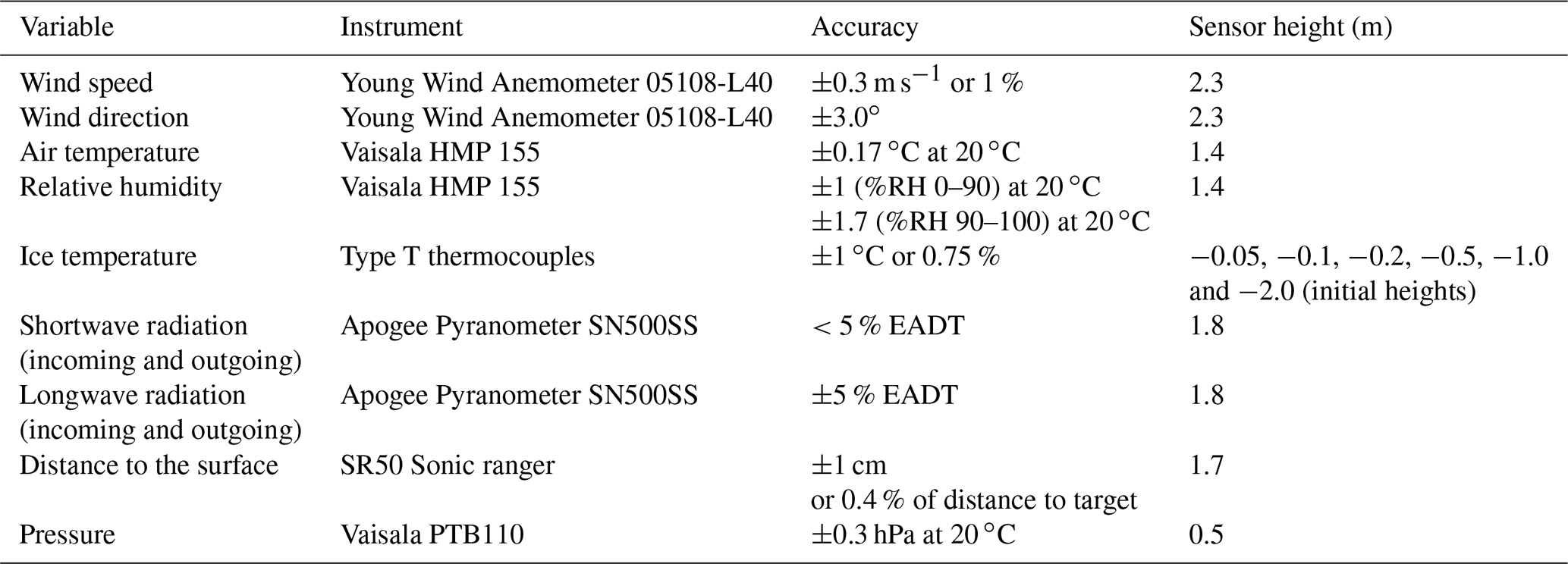
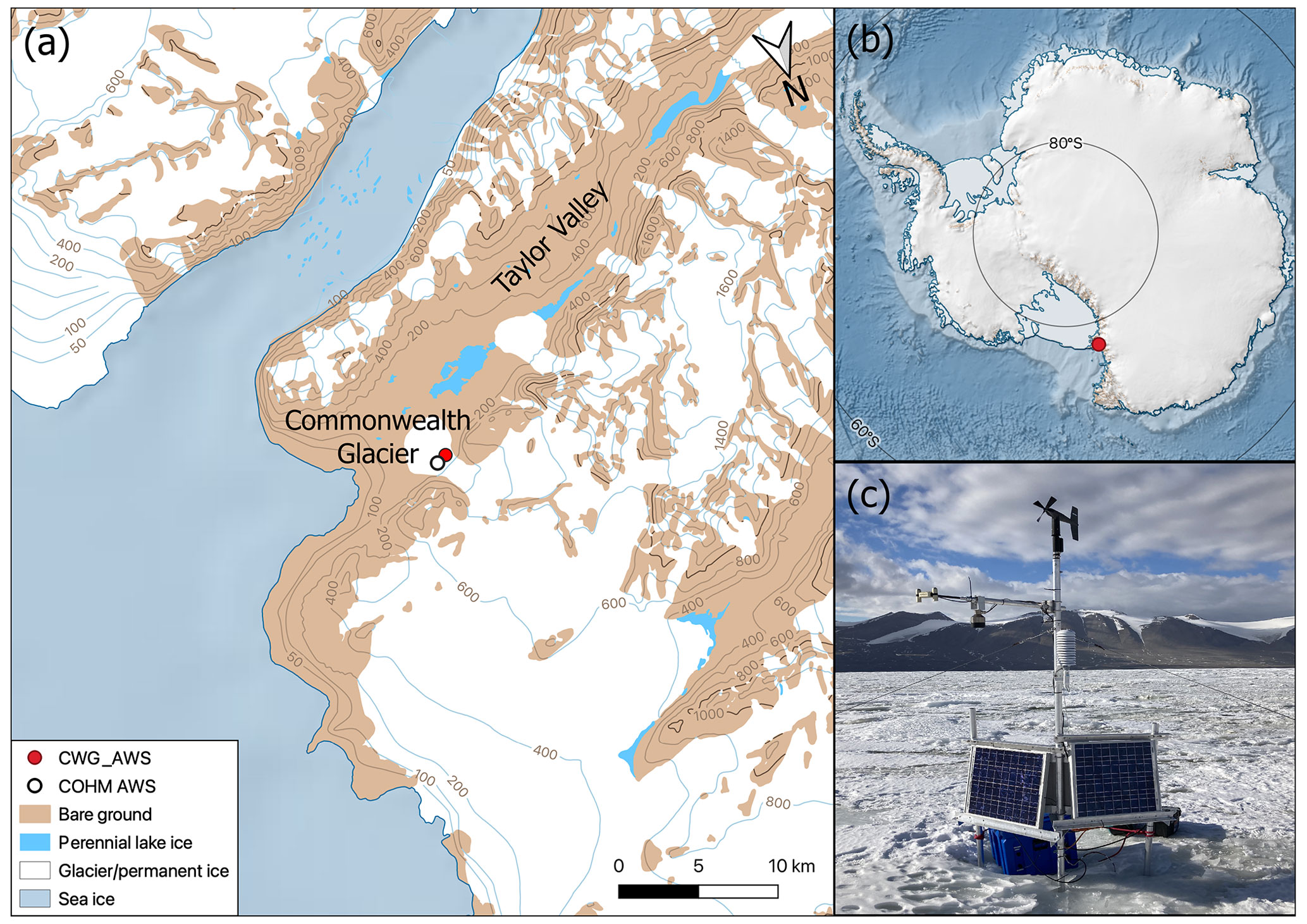
Figure 2(a) Map of Commonwealth Glacier with respect to Taylor Valley with CWG AWS in the red-filled circle. COHM AWS is indicated by a black open circle located 140 m to the east of CWG AWS. (b) Taylor Valley with respect to the continent. (c) The CWG AWS on 31 January 2022. Detailed base maps from RAMP2 Hillshade, ETOPO1/IBCSCO/RAMP2 Hillshade and the Elevation model. This map was made using the Quantarctica QGIS package collated by the Norwegian Polar Institute (https://www.npolar.no/quantarctica/, last access: 9 April 2023).
The MDV Long Term Ecological Research Project station on Commonwealth Glacier (COHM AWS) is located at −77.563712, 163.280145∘and 290 m in elevation (Doran and Fountain, 2022). COHM AWS is located 140 m east of CWG AWS. The accuracy of the sensors is similar to CWG AWS, and the instruments are detailed in Gooseff et al. (2022).
3.3 Model forcing
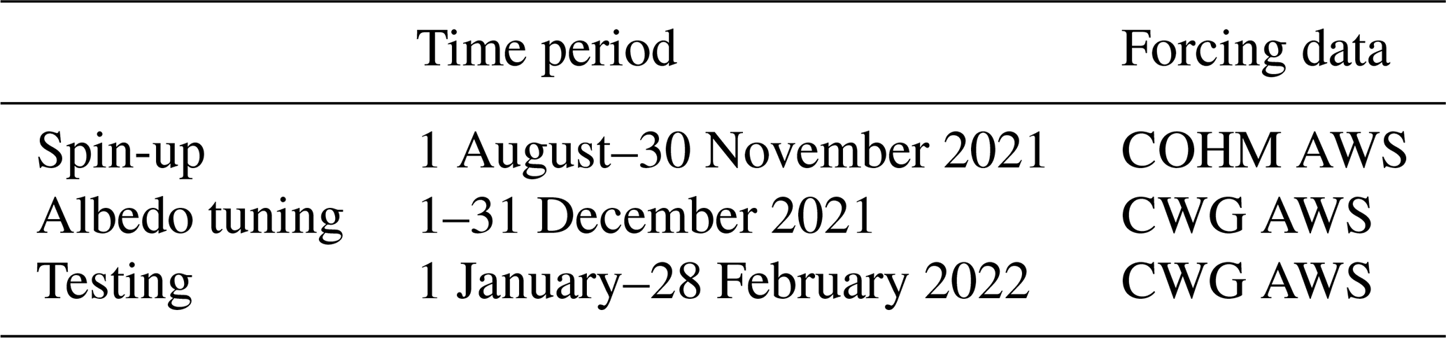
The model is forced at an hourly time step by observational data from the COHM AWS and the CWG AWS. For the model spin-up, the MDV Long Term Ecological Research Project station on Commonwealth Glacier (COHM AWS) (Doran and Fountain, 2022) is used because it is before the CWG AWS was installed. The time periods and forcing data used are shown in Table 2.
Table 2Summary of the time periods and forcing data used for the model experiment.
The following meteorological variables were used: incoming shortwave radiation (W m−2), incoming longwave radiation (W m−2), air temperature at 2 m (K), the meridional and zonal wind vector components (m s−1), specific humidity (kg kg−1), surface pressure (hPa) and precipitation (mm w.e. s−1). The data from the AWSs were processed similarly to Gillett and Cullen (2011), where specific humidity was calculated with respect to water and ice depending on whether the air temperature was above or below the melting point. Pressure for the spin-up period was obtained from the nearest grid cell to the CWG AWS in Antarctic Mesoscale WRF Prediction System (AMPS) atmospheric data as there was no barometer at the COHM AWS.
Given that there was no precipitation sensor at either AWS, precipitation was obtained using changes in snow height measurements from the SR50 sensor at the COHM and CWG AWSs. Fountain et al. (2010) calculated precipitation in the MDV by taking the daily average change in snow height. If the change in snow height between days was greater than 5 mm, this was taken as precipitation. We attempted this method by Fountain et al. (2010) but found that it filtered out all of the summer snowfall events (some of which were witnessed during field work). Instead, we opted to fit a k-nearest neighbour regression (n=30 and uniform weights) to the 30 min snow height time series in order to filter out the noise from the sensor. This method is similar to a rolling mean and smooths the snow height time series. Values below 0.3 mm (0.4 mm for January and February) of change in snow height during the 30 min period were removed to filter noise from the sensor. This threshold was tuned to observations of snow events from the 2021/22 field campaign and observed albedo. Next, the positive increases in the hourly sum of surface height change were converted (mm w.e.) using a fresh snow density of 150 kg m−3 to convert height change to the mass of snow.
The forcing data are displayed in Fig. 3. Meteorological conditions vary seasonally with a stark difference in incoming shortwave radiation between the polar night and summer. This controls the surface temperatures that vary between the melting point in the summer and a minimum of −43 ∘C in August, which is often the coldest month in the MDV. Relative humidities are low and snowfall amounts are very low, with a higher frequency near the middle of the summer. Wind direction varies between north-easterlies (sea breeze), northerlies (down-glacier katabatic) and westerlies (föhn), with the greatest wind speeds occurring when there is a westerly. The average pressure over the period is 950 hPa.
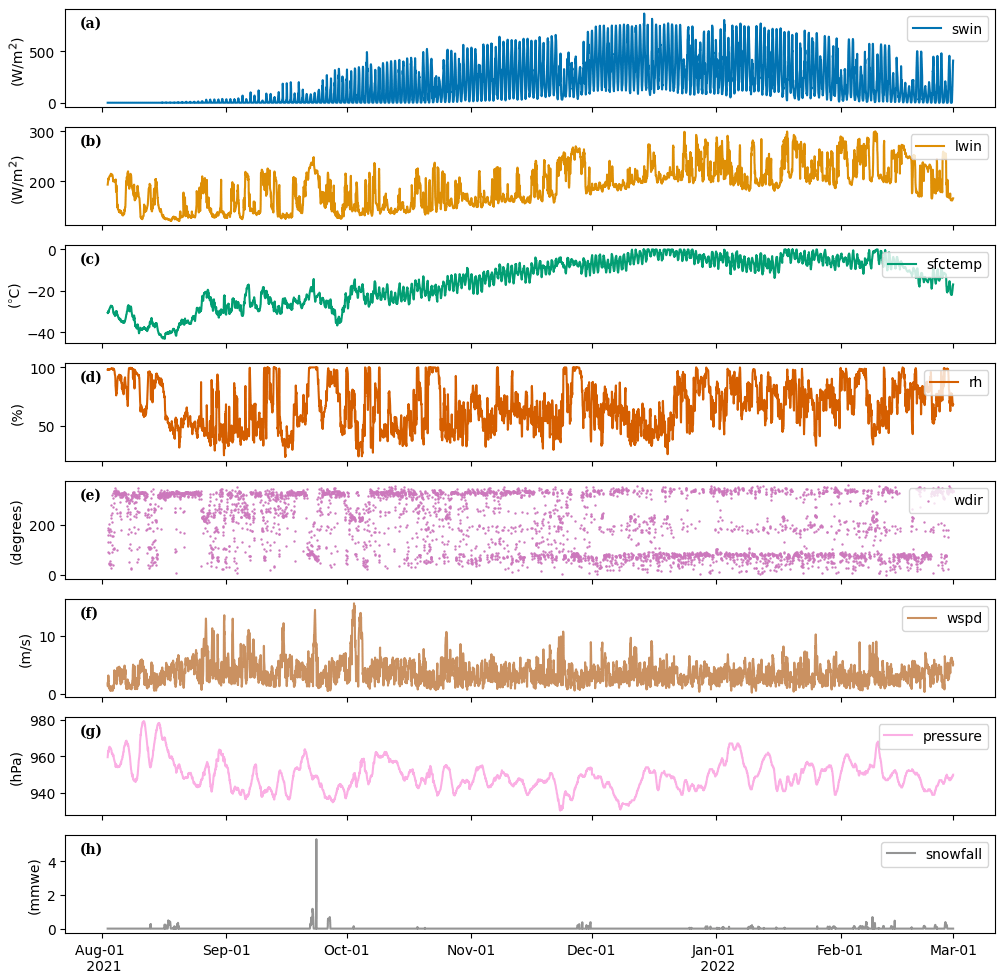
Figure 3(a–h) Average hourly incoming shortwave radiation, incoming longwave radiation, surface temperature, relative humidity, wind direction, wind speed, surface pressure and snowfall measured at COHM AWS (1 August to 30 November 2021) and CWG AWS (1 December 2021 to 28 February 2022). Pressure is from the Antarctic Mesoscale WRF Prediction System (AMPS) for the first period as it was not measured at COHM AWS.
Comparing the 2021/22 season to the 1999–2022 long-term average over December and January (Hofsteenge et al., 2023), we find that air temperature, wind and albedo were close to the average. Air temperatures were 0.2 ∘C below the average, wind speed was 0.1 m s−1 below the average and albedo was 0.02 below the average. There was slightly less cloud cover as incoming shortwave radiation was 43.4 W m−2 (13.9 %) above the average and incoming longwave radiation was 6.9 W m−2 (−3.0 %) below the average.
3.4 Implementation and initialization
In this model experiment, we used the Crocus snowpack model embedded in WRF-Hydro/Glacier version 5.2.0 (Eidhammer et al., 2021). Crocus was forced by observed meteorological data at an hourly time step and was analysed at a point on Commonwealth Glacier. The high-quality observational data obtained on Commonwealth Glacier reduce uncertainty that might be introduced by using model or gridded data as meteorological forcing data. Crocus was initialized with 40 layers (as in Eidhammer et al., 2021) and a constant thickness of 50 m for simplicity, in line with terminal cliff height observations. Snow depth was initialized as 0 m and the layers were initialized with a constant density of 900 kg m−3. The glacier temperatures were initialized at −18 ∘C for each layer and with a constant temperature of −18 ∘C at the soil–glacier boundary since the temperature at this depth is expected to be the annual mean air temperature (Fountain et al., 1998). More information on the model configuration can be found in the namelists provided in the Code and data availability section.
The WRF-Hydro/Glacier spin-up period was 1 August to 30 November 2021 to obtain a realistic ice temperature profile at the start of the simulation. We analysed ice temperatures at the end of the spin-up period and found that the differences between observed and modelled ice temperatures at depths of 0.05, 0.1, 0.2, 0.5 and 2.0 m at the beginning of December were less than 1 ∘C, which is within the sensor uncertainty shown in Table 1. Given this agreement, we concluded that the spin-up time is sufficient for the model testing in this evaluation (see Sect. 5.2 for further discussion). Following the spin-up period, the different model configurations were validated from 1 December 2021 to 28 February 2022. This period was chosen because there are no observed streamflow measurements outside of these months. Ice surface temperatures reach the melting point for the first time in December and the temperatures switch to a primarily cooling regime in February, descending well below the melting point.
3.5 Validation data
WRF-Hydro/Glacier is validated using surface temperature, internal ice temperatures, albedo, surface height change and streamflow over the melt season. Ice surface temperature was calculated from outgoing longwave radiation (Table 1) using the Stefan–Boltzmann law and an emissivity of 1. Ice temperatures were obtained from thermocouples deployed at six different depths (Table 1). A 2-week validation period in early December was chosen as the top two thermocouple sensors melted out after the first 2 weeks of December. Observed albedo was calculated as accumulated albedo by taking a moving mean over 24 h for the ratio of accumulated outgoing shortwave radiation (absolute value) over accumulated incoming shortwave radiation (Van Den Broeke et al., 2004). This method is used in polar regions to limit uncertainty associated with a changing solar zenith angle with the midnight sun. As noted in Sect. 3.3, surface height change was obtained using the k-nearest neighbour regression used for pre-processing precipitation to eliminate noise from the sensor. Finally, streamflow data came from the Lost Seal stream gauge (Gooseff and Mcknight, 2021) and were used to validate the temporal variation in simulated runoff.
4.1 Water drainage through snowpacks or glaciers
Eidhammer et al. (2021) implemented WRF-Hydro/Glacier on a temperate glacier in Norway with internal temperatures initialized at 0 ∘C. Runoff in the summer is generated by precipitation (rain) in addition to melt. In contrast, the MDV glaciers are cold-based with internal temperatures around −18 ∘C, and runoff is entirely from surface and near-surface glacial melt. Due to the extreme differences in these two environments, modifications to the water flow through snowpack and ice were necessary in order to adapt Crocus embedded in WRF-Hydro/Glacier to this environment.
As a snowpack model, runoff in the original WRF-Hydro/Glacier is calculated as the remaining water after it has percolated through all of the layers and reached the ice–soil interface. In this version of the model, ice is not treated differently to snow layers and the ice remains porous. This is problematic as it allows meltwater to percolate through the ice layers rather than having the ice layers act as a barrier (MacDonell, 2008; Bergstrom et al., 2021). As the water percolates, it can refreeze in a layer depending on temperature and energy or it can be held in the layer as liquid water content. Figure 4a depicts the water flow scheme from WRF-Hydro/Glacier (oldrunoff) for a single hour in the top 40 cm or four layers of the glacier. Figure 4a shows that meltwater is generated in the first layer, and a portion of that melt is held in the layer as liquid water content since it is a snow layer. The remaining meltwater percolates down to the second layer, which is an ice layer. Some of the percolated water refreezes and a smaller amount is held as the liquid water content of the layer. Any remaining water continues to percolate to the third layer, where all of it refreezes, and thus there is no runoff.
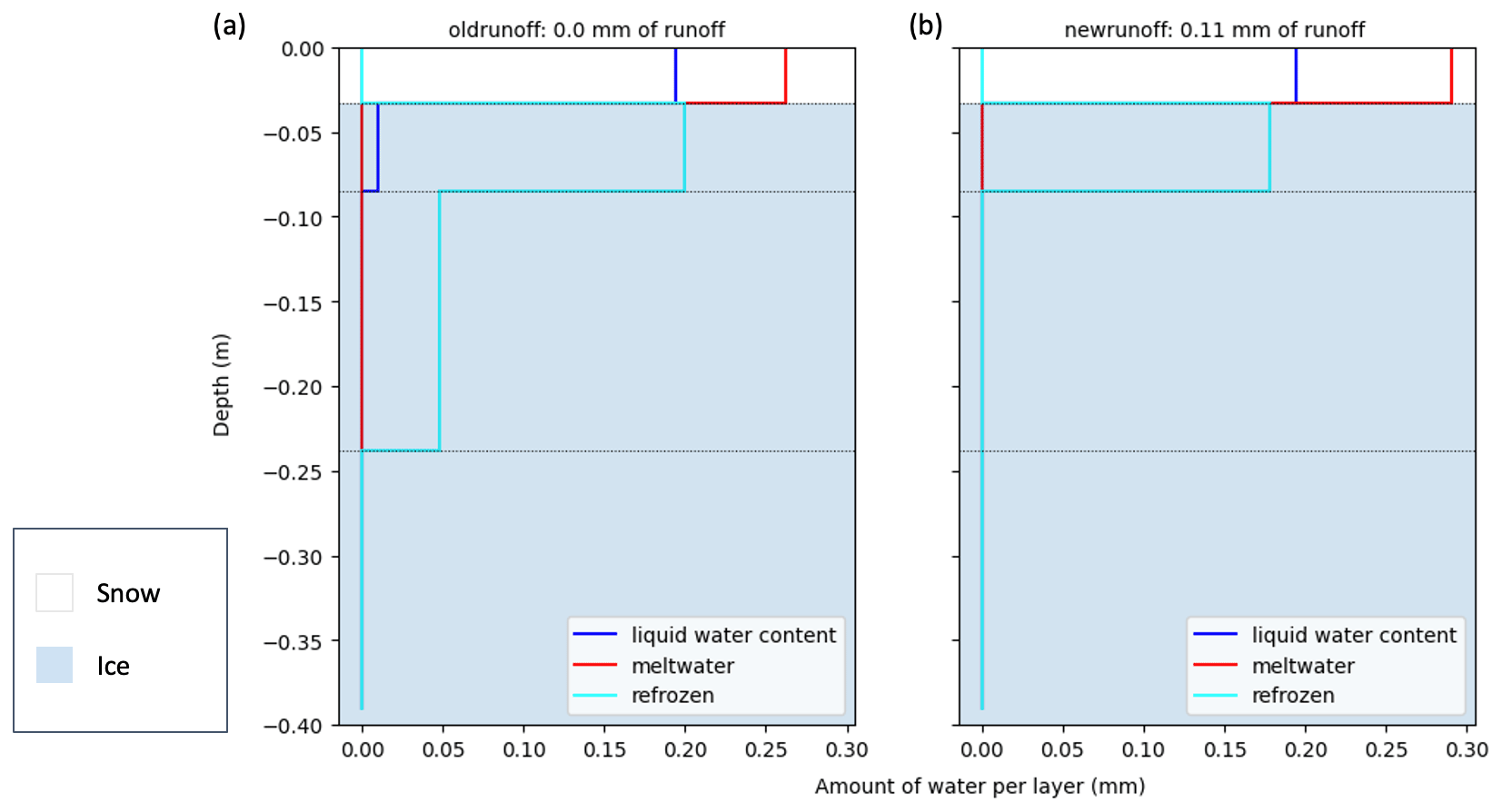
Figure 4A comparison between the (a) original runoff scheme from Crocus (oldrunoff) and the (b) new modified runoff scheme (newrunoff). Cross sections show the top 40 cm and the total amount of liquid water held in the layer (blue), the total amount of water melted (red) and the total amount refrozen (cyan) for each layer at 03:00 UTC on 10 December 2021. The white and blue background colours show which layers are snow and ice, respectively. Horizontal black dotted lines denote the different layers.
Runoff is only possible in oldrunoff if the entire glacier is at the melting point such that the liquid water can percolate through the entire glacier or snowpack column. This does not align with MDV observations of near-surface melt with steep subsurface temperature gradients (Fountain et al., 1998; Hoffman et al., 2014). Thus, we introduce a condition such that if the liquid water reaches an ice layer, a portion refreezes and all remaining water becomes runoff. This allows the ice to be a barrier and results in the generation of near-surface runoff. The effect of this modification can be seen in Fig. 4b, newrunoff. Here, the top snow layer is similar to Fig. 4a, and a portion of the water that percolates through the top snow layer refreezes in the second layer. The difference is that there is no liquid water held in the second layer, since the ice layers are no longer porous and have a liquid-water-holding capacity of zero. The remaining liquid water from the second layer becomes runoff since the ice layer is a barrier preventing further percolation. Thus, there is 0.11 mm of runoff in newrunoff.
4.2 Crocus spectral albedo scheme in WRF-Hydro/Glacier
4.2.1 Description of the albedo scheme
The Crocus albedo scheme implemented in WRF-Hydro/Glacier is currently calculated over three spectral bands, where Band 1 is the visible band with wavelengths from 0.3 to 0.8 µm, Band 2 is the red band with wavelengths from 0.8 to 1.5 µm and Band 3 is the near-infrared band with wavelengths from 1.5 to 2.8 µm. The albedo in each band is calculated for the top two layers of the glacier using different schemes for ice and snow.
The Crocus snow albedo scheme in WRF-Hydro/Glacier is based on the theoretical study of Warren (1982). Albedo for each band (i=1…3) of the two top layers () is calculated in the following equations.
S are various snow model parameters (see Table 3), dopt is the optical diameter of the snow grains, P is the mean surface pressure in hectopascals, A is the snow age in days and d′ is the minimum of and 0.0023 for each layer, j. All of the constants in the three equations correspond to parameters that can be altered in the Crocus namelist (see Table 3).
Table 3Parameters from the original Crocus in WRF-Hydro/Glacier (oldalbedo) compared to the new scheme (newalbedo). Bold indicates changed parameters. We introduce a new parameter, XVALB12 (S2a), to specify the minimum albedo for Band 2 as the original value was hard-coded.
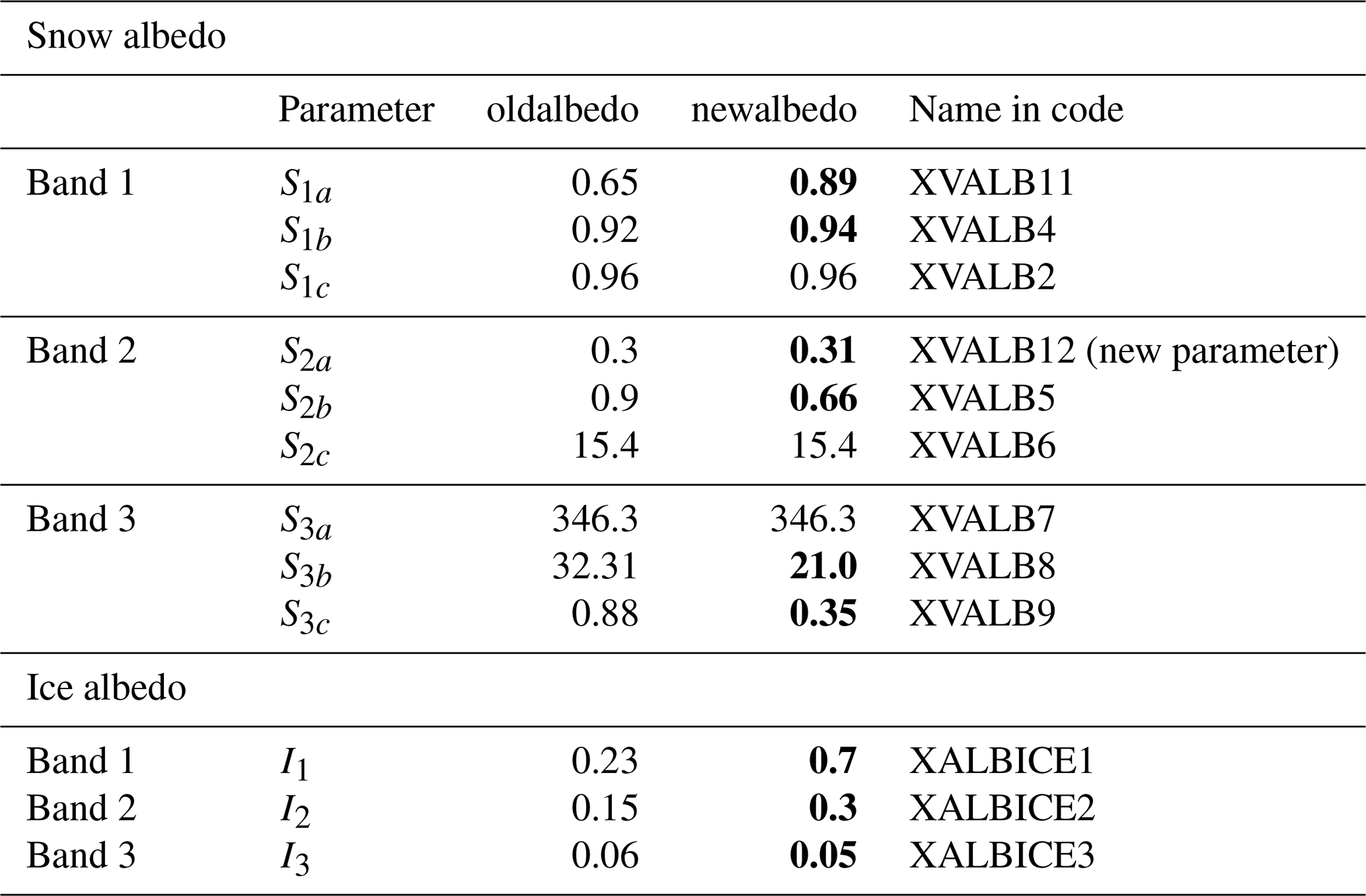
For ice layers (density >850 kg m−3), the albedo of the three bands is
Ii are the constant values for ice for the three bands (i) listed in Table 3.
Next, a weight (f) is calculated for both layers as a function of the thickness of each layer and various parameters:
where Δz1 is the thickness of the first layer. The total albedo of each band (αi) is then
and the broadband albedo is a weighted average of the total albedo of each band:
4.2.2 Motivation for tuning the parameters
Figure 5 shows the observed broadband albedo from 1 December to 28 February. There was snowfall at the end of November (Fig. 3h), so on 1 December the time series begins with snow that is no longer fresh. The surface has a broadband albedo of 0.7, and then the surface transitions from snow to ice on 20 December with an albedo of 0.55. Afterwards, there are a few snowfall events (e.g. 24, 26 and 30 December and 5 and 11 January) that increase albedo, followed by a slow decay after each snowfall. Looking at modelled albedo, oldalbedo (Fig. 5) begins with a snow albedo of 0.81, and then the surface transitions to ice with a constant albedo of 0.2 on 13 December. Each time it snows, the albedo increases briefly and then rapidly decays to ice.
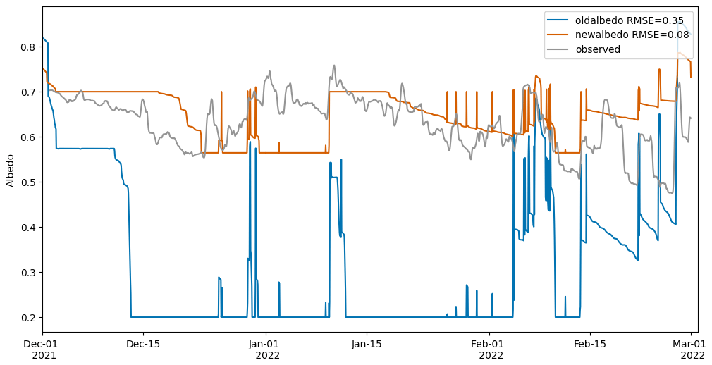
Figure 5Comparison between the broadband albedo of the original Crocus scheme (oldalbedo) in blue, the modified scheme (newalbedo) in orange and the observed daily accumulated albedo in grey.
The issues are that (1) the modelled ice albedo is too low compared to the observations (0.2 vs. 0.55) and that (2) the modelled snow albedo does not match the observations (0.7 vs. 0.81). The observed ice albedo only decreases to 0.48 and is similar to the range of minimum albedo measured by Bergstrom et al. (2020) of approximately 0.4–0.5 on Commonwealth Glacier over three melt seasons. Hoffman (2011) similarly found a minimum albedo of ∼ 0.53. These values are higher than temperate glaciers because of minimal sediment and impurities on the glacier and low amounts of meltwater present that can lower albedo (Hoffman, 2011). The snow albedo observations at the beginning of the period are lower than the modelled snow albedo. Observed snow albedo over the melt season is also similar to the albedo observations from Bergstrom et al. (2020). However, the values for fresh snow are often lower than those observed in other glaciated locations. For example, Reijmer et al. (2001) recorded an average snow albedo of 0.78 at a point in Dronning Maud Land, Antarctica, whilst the average snow albedo in this study is ∼ 0.65. This is likely because there are very little snowfall amounts in the MDV, and the albedo will be a combination of thin surface snow and the lower albedo of the ice beneath. The parameters in the model snow albedo scheme are based on modelled snow albedo in Warren (1982) and the parameters are optimized for the French Alps (Brun et al., 1992). The ice albedo scheme is constant and the parameters have been tuned to glaciers in the French Alps (Gerbaux et al., 2005). Thus, the parameters of the model albedo scheme must be modified to better represent the conditions found on the glaciers in the MDV.
4.2.3 Modifying the albedo scheme parameters
We chose to tune the albedo scheme for December 2021 and test the new parameters from 1 January to 28 February 2022. In this study, we opted to use observed spectral albedo profiles measured by Dadic et al. (2013) in Allan Hills, East Antarctica, as they provide similar information to Warren (1982) but for a location that is closer to our field site on Commonwealth Glacier.
First, we determine new parameters for the ice albedo bands by calculating the average spectral albedo of each band from Dadic et al. (2013, Fig. 6) for the different types of ice (white and blue ice). These values were then tuned to the minimum observed broadband albedo during December 2021 whilst ensuring that the value of each band remained in the range of average values from Dadic et al. (2013). The effect of this tuning process for ice albedo is shown from 13 to 25 December in Fig. 5, where newalbedo is much closer to the broadband albedo observed on the ice surface in this period.
Next, we modified the maximum and minimum spectral albedo in each band based on observations by Dadic et al. (2013) (S1b and S1a, S2b and S2a). Band 3 is slightly more complex. Here, we solved a system of equations using the largest and smallest optical diameters from oldalbedo to represent snow and firn over the tuning period. These maxima and minima were constrained by averages calculated from Fig. 6 in Dadic et al. (2013) for snow and firn and tuned to observed broadband albedo (S3b and S3c). The new parameter choices are in bold in Table 3. Figure 6b shows the effect of the new parameters on the three bands and the broadband albedo over the full melt season. Bands are separate in newalbedo and are aligned with theory as well as observations from Dadic et al. (2013). Variability in observed albedo is better captured by newalbedo over the melt season with a root mean square error of 0.08 compared to oldalbedo with a root mean square error of 0.35. Accurately simulating albedo enables us to better simulate the feedbacks between albedo, precipitation and melt.
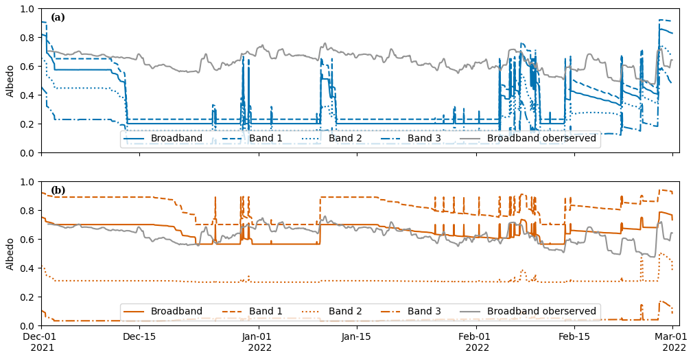
Figure 6Comparison between the daily accumulated broadband albedo in grey and the three spectral albedo bands of (a) the original Crocus albedo (oldalbedo) in blue and (b) the modified scheme (newalbedo) in orange.
In this section, we evaluate three different versions of the model code representing the original scheme (oldrunoff_oldalbedo), updates to both runoff and albedo schemes (newrunoff_newalbedo) and updates only to the runoff scheme (newrunoff_oldalbedo).
5.1 Surface temperature
Figure 7 shows the performance of the different models compared to the observed surface temperatures at the AWS over the second half of December. The time series shows that the newrunoff_newalbedo daytime surface temperature drops below the melting point from 26 to 30 December similarly to observed surface temperatures, while the two previous versions of the model (oldrunoff_oldalbedo and newrunoff_oldalbedo) reach the melting point daily during that period. This is more evident in Fig. 8, where the two models using the original albedo scheme have similar root mean square errors (Fig. 8a, b). However, the root mean square error of newrunoff_newalbedo (Fig. 8c) is 60 % less than newrunoff_oldalbedo and 62 % less than oldrunoff_oldalbedo. Furthermore, newrunoff_newalbedo has a more equal spread on either side of the 1 : 1 line around the melting point compared to the two models with the original albedo scheme, which both overestimate the number of hours with surface temperature at the melting point as seen by the aggregation of points in the top left of the 1 : 1 line (Fig. 8a, b). The percentage of time each model is at the melting point is 25.8 % (557.3 h) for oldrunoff_oldalbedo, 24.5 % (529.2 h) for newrunoff_oldalbedo and 5.7 % (123.12 h) for newrunoff_newalbedo compared to 5.0 % (108.0 h) for observed surface temperatures. In comparison, Hoffman et al. (2014) found that, on average, there were 255.1 h of surface and near-surface melt with a maximum of 452 h and a minimum of 92 h from 1996 to 2009 on Taylor Glacier. Thus, the values for newrunoff_newalbedo are similar to the average, while oldrunoff_oldalbedo and newrunoff_oldalbedo are greater than the maximum number of hours found by Hoffman et al. (2014).
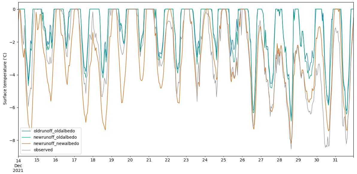
Figure 7Comparison between the three different versions of the model and the observed surface temperatures over the last 2 weeks in December 2021.
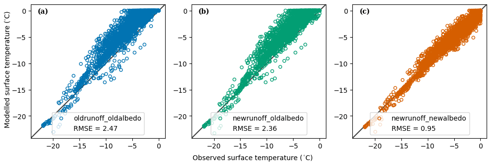
Figure 8A scatter plot with modelled surface temperatures vs. observed surface temperatures for the three models from 1 December 2021 to 28 February 2022.
For temperatures around −20 ∘C, newrunoff_newalbedo has a cold bias of up to 2 ∘C, which can also be seen in the daily minima in Fig. 7. This is likely due to the observed albedo being lower than the modelled albedo during this period, as seen in Fig. 5.
5.2 Internal ice temperatures
Internal ice temperatures at six different depths are validated for the three model runs in Table 4. This shows that newrunoff_newalbedo has the lowest root mean square errors for internal ice temperatures at TC1–4 and TC6. Figure 9 shows the temporal variability of the modelled vs. observed ice temperatures for newrunoff_newalbedo. The modelled temperatures agree with the measured temperatures and are often within 1 ∘C of the measurement. The root mean square errors for TC2–6 all lie below one except for TC1, which matches observations at the beginning of the period but has a cold bias and a phase shift later in the period. The first time step of the period beginning on 1 December shows that the model is in good agreement with the observations and gives us confidence that a longer spin-up is not necessary. The model also captures both the diurnal cycle and the seasonal warming seen in TC4, TC5 and TC6. This can also be seen in Fig. 10, which shows a cross section of ice temperatures in the top 3 m of the glacier modelled by newrunoff_newalbedo from August 2021 to February 2022. Darker blues indicate the cooling of the glacier during the spin-up period (August–November 2021) and then the warming period beginning in December. However, there is a slight delay in the diurnal cycle of the measurements compared to the model in Fig. 9. This could be due to differences in solar-penetrating radiation that result in the glacier not warming enough compared to the measurements. Overall, the model does a satisfactory job of modelling the near-surface ice temperatures as seen in the root mean square errors in Fig. 9, which is important for generating near-surface melt.
Table 4Root mean square errors of the internal ice temperatures of the three model versions at six different depths from 1 to 15 December 2021.
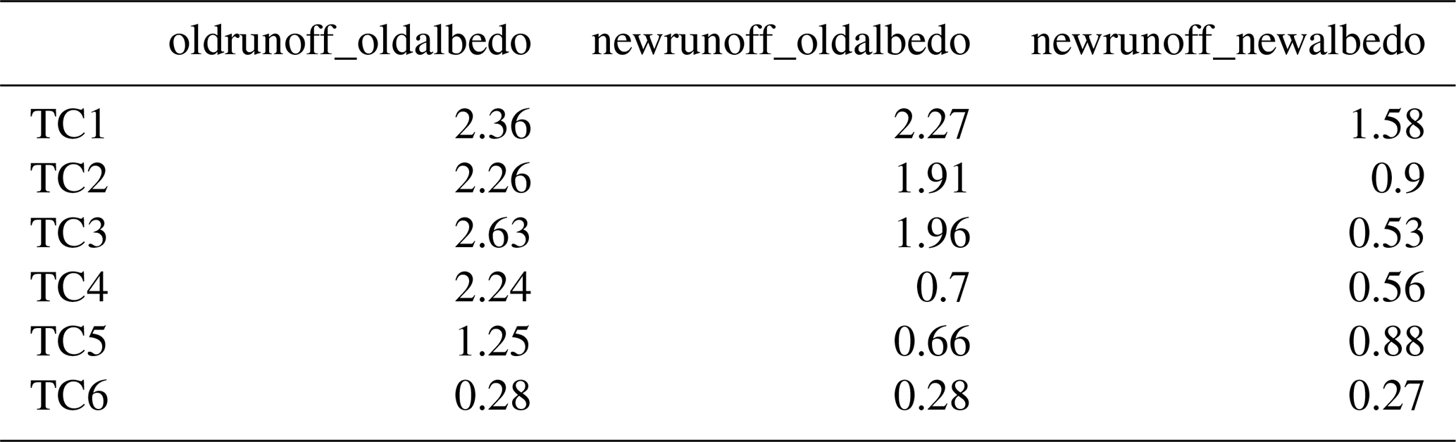
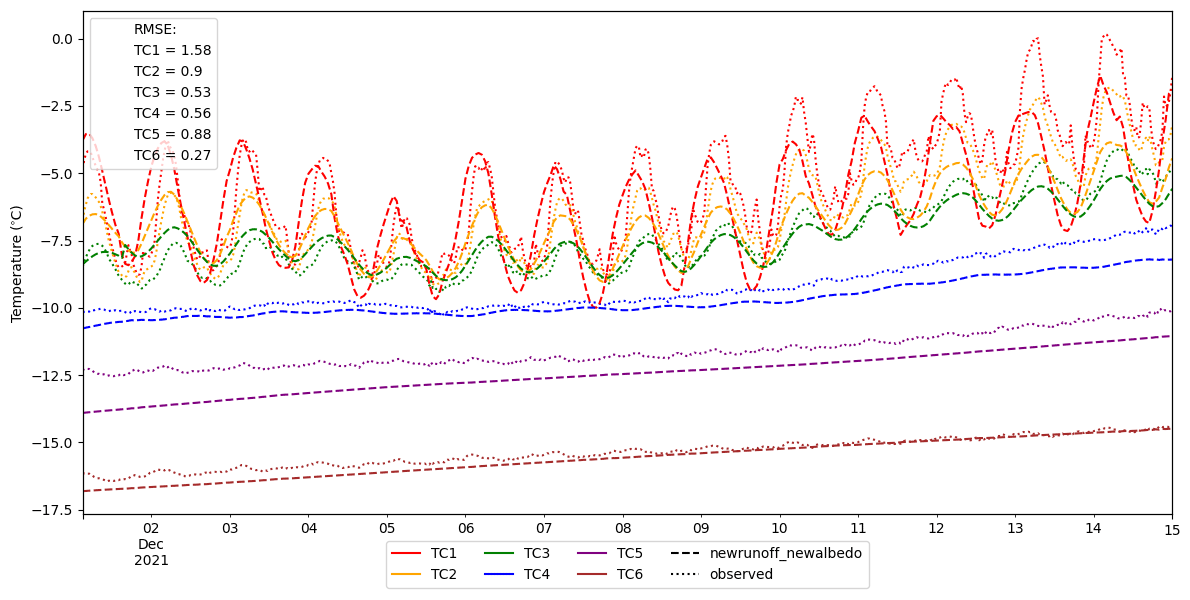
Figure 9Modelled internal ice temperatures from newrunoff_newalbedo for 1–15 December 2021. Thermocouples were initially deployed at six different depths: 0.05, 0.1, 0.2, 0.5, 1.0 and 2.0 m. Note that the measurements are not at a constant depth with time as the sensors were melting out over the period. This shows diurnal variability at shallower depths and the seasonal warming wave below.
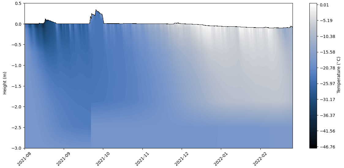
Figure 10Cross section of modelled temperature from newrunoff_newalbedo of the top 3 m of the glacier over the spin-up period of August–November and the validation period of December–February. This shows the diurnal variability at shallower depths, the seasonal cooling and then warming waves below.
5.3 Surface height change
Figure 11 shows the surface height change from 1 December 2021 to 28 February 2022 of the three model versions compared with observations of surface height. Although the three models begin in December in alignment (same spin-up), they begin to diverge a couple of days later. The model that is most similar to the observed surface height is newrunoff_newalbedo with a root mean square error of 0.02. The model that performs the worst is oldrunoff_oldalbedo with a 35 cm more decrease in surface height than the observations over the 3-month period and a root mean square error of 0.26. The performance of newrunoff_oldalbedo is similar to newrunoff_newalbedo but with a root mean square error of 0.05.
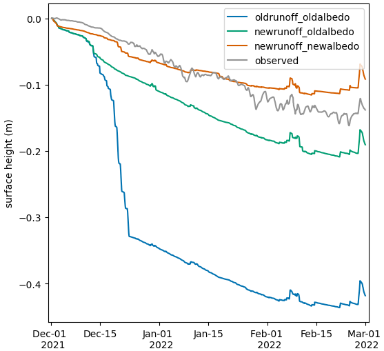
Figure 11The change in surface height (m) between the three models and the quarter-hourly observational data.
The differences between the surface height change in the three models occur during the first 3 weeks of December. After 23 December, the rate of decrease in the change in surface height across the three models stabilizes. From this point to the end of the simulation, oldrunoff_oldalbedo has 90 cm ablation, while newrunoff_oldalbedo has 10 cm ablation and newrunoff_newalbedo has 3 cm ablation compared to 10 cm observed ablation. On 6 December, oldrunoff_oldalbedo and newrunoff_oldalbedo reach the melting point for the first time and the surface height decreases more quickly than newrunoff_newalbedo. On 13 December, TC1–3 near-surface ice temperatures of oldrunoff_oldalbedo reach the melting point (Fig. A1), whilst newrunoff_oldalbedo near-surface ice temperatures remain below the melting point (Fig. A2). This rapid decrease in surface height and warming of the glacier layers for oldrunoff_oldalbedo may be due to near-surface melt that is percolating through ice layers and subsequently warming them rather than draining as near-surface runoff as modified in newrunoff_oldalbedo. This can be seen in Fig. A1 for oldrunoff_oldalbedo, where TC1 reaches the melting point on 12 December, followed by internal ice temperatures for TC2–5 increasing rapidly from 13 December. On the other hand, in Fig. A2, TC1 from newrunoff_oldalbedo reaches the melting point on 13 December, but TC2–5 do not increase as much as in oldrunoff_oldalbedo. Thus, it is evident that optimizing the parameters for the albedo scheme and modifying the drainage through the glacier were needed to accurately simulate surface height change.
5.4 Runoff
Although we do not have site-specific runoff measurements for this location, stream gauge observations of the Lost Seal catchment on Commonwealth Glacier (Gooseff and Mcknight, 2021) indicate that melt and runoff are activated episodically rather than consistently melting daily over the melt season (Fig. 12c). Figure 12a shows the daily accumulated runoff (mm) of liquid water for the three different models. There is no runoff from oldrunoff_oldalbedo during the entire period of the melt season due to the percolation and subsequent refreezing of meltwater through the ice layers that was modified for the newrunoff models. In comparison, from 10 December runoff is generated almost daily throughout the season in newrunoff_oldalbedo, with a daily maximum of 45.0 mm, whereas runoff is more episodic in newrunoff_newalbedo, with a daily maximum of 5.1 mm.
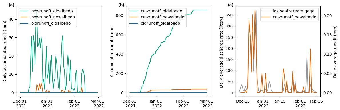
Figure 12(a) Daily accumulated runoff and (b) cumulative runoff from the three model runs from 1 December 2021 to 28 February 2022. (c) Daily average discharge from the Lost Seal stream gauge (grey) compared to modelled daily average runoff (orange) from newrunoff_newalbedo.
Figure 12a, b show that the runoff is generated earlier and is larger in newrunoff_oldalbedo than newrunoff_newalbedo. This is because the albedo falls to the ice albedo on the day that runoff is activated for the season (Fig. 5). There is less runoff overall in newrunoff_newalbedo and runoff drops to zero (frequently compared to newrunoff_oldalbedo), which has runoff every day from the start to the end of the season. When we compare the runoff with surface temperatures from Fig. 7, it can be seen that runoff is activated when ice surface temperatures reach the melting point and the runoff shuts off when the temperature drops below the melting point.
Furthermore, we can compare the daily average modelled runoff from newrunoff_newalbedo to the daily average stream gauge observations (Gooseff and Mcknight, 2021) in Fig. 12c. Although we cannot compare the magnitudes, this shows that we are accurately capturing the temporal variability and the episodic nature of melt (Fig. 12c). Modelled runoff does not account for the physical processes of water drainage off-glacier, such as evaporation or soil absorption, and this may explain some of the differences between the stream gauge and the model. Hoffman et al. (2014) calculated a range of 11.2 to 152.0 mm w.e. of total subsurface drainage and surface melt per melt season over 13 years at a point on Taylor Glacier. The total runoff over the melt season in our study was 0 mm w.e. for oldrunoff_oldalbedo, 858 mm w.e. for newrunoff_oldalbedo and 36 mm w.e. for newrunoff_newalbedo. The total runoff for newrunoff_newalbedo falls in the range from Hoffman et al. (2014). Thus, we are confident that newrunoff_newalbedo models the frequency and magnitude runoff accurately.
5.5 Limitations
We implemented the WRF-Hydro/Glacier model at a point on Commonwealth Glacier and forced the model with observational data in order to limit the input uncertainties to the model that would be introduced when using atmospheric model or gridded data. However, a few uncertainties in the input data still exist, especially regarding precipitation. Precipitation was calculated from the change in snow height record, but this was challenging as the data are noisy and summer snow accumulation is very small, increases albedo and pauses melt generation (Fountain et al., 2010). Temperature and wind speed can impact the sonic ranging sensor that measures the snow height and contributes to the noise in the data. The threshold for snow was tuned on a monthly basis and was smaller than both the instrument accuracy and the thresholds from Fountain et al. (2010) and Myers et al. (2022), which would have filtered out all of the summer snowfall events seen in the observed albedo.
Other limitations to this study are the short time period used for spin-up, tuning and testing of WRF-Hydro/Glacier. We demonstrate that the 4-month spin-up is sufficient to accurately simulate the internal ice temperatures. Although a longer time period could be helpful for tuning and testing the model, this study is a proof of concept, and the evidence provided demonstrates that 1 month of tuning is sufficient to simulate the evolution of the broadband albedo for January and February.
To better understand the physical processes governing the hydrological cycle in the MDV, it is necessary to resolve the connections between the atmosphere, glaciers, bare land, stream channels and lakes (hydrological reservoirs). What makes the MDV unique compared to other glaciated environments is that changes in surface energy balance are the primary control on meltwater generation and mass balance, as precipitation is limited. Although previous studies have implemented surface energy and mass balance models on glaciers in the MDV (Hoffman, 2011; Macdonell et al., 2013; Hofsteenge et al., 2022), they have not been able to fully account for the stream channels and streamflow from the glaciers to the surrounding landscape. By implementing a new modelling framework that couples a detailed snowpack model to a fully distributed hydrological model (WRF-Hydro/Glacier), we have taken the first step in enabling the hydrological connectivity of the MDV to be further assessed.
To successfully simulate the onset, duration and end of melt on a cold-based glacier in the MDV, the multi-layer snowpack scheme in WRF-Hydro/Glacier needed to be optimized, which was achieved at a point scale over a 7-month period encapsulating a melt season. The snowpack model (Crocus), which is embedded in WRF-Hydro/Glacier, was (1) modified to limit the percolation of meltwater in the presence of ice layers and (2) optimized to improve the parameter set controlling albedo and net shortwave radiation. We demonstrate that simulating albedo, which has not been attempted before on a glacier in the MDV, is necessary to resolve the complex feedbacks between albedo, snowfall and melt in this energy-limited environment. Our approach to simulate albedo based on the evolution of snow grain properties is a significant step forward for modelling glacier response to climate change in the MDV compared to using point-based observations of albedo (e.g. Hoffman, 2011; Hofsteenge et al., 2022).
Future research will be able to utilize this modelling framework to better resolve the spatial and temporal variability in albedo, which is critical in governing spatially distributed melt and hydrological connectivity in the MDV. For example, Bergstrom et al. (2020) measured the spatial variability of albedo from a series of radiometric observations obtained from helicopter flights over three MDV glaciers, which showed that albedo not only increased with elevation, but also increased from west to east across both the Canada and Commonwealth glaciers in Taylor Valley. The longitudinal patterns in albedo observed by Bergstrom et al. (2020) demonstrate that point-based observations of albedo are not sufficient to resolve the spatial and temporal variability in albedo. Thus, the optimized simulation of albedo in the multi-layer snowpack scheme in WRF-Hydro/Glacier used in this study provides a new pathway to resolve this observed complexity, which is critical in governing the amount of meltwater generated from glaciers in the MDV. Importantly, it provides us with confidence that we have developed a modelling framework that will enable us to get the “right answers for the right reasons” (Kirchner, 2006) in regard to resolving one of the key physical processes governing the spatial variability of melt.
The modified WRF-Hydro/Glacier model will also allow us to expand on the work of Hoffman (2011) and Cross et al. (2022) by accounting for in-stream processes such as evaporation and soil absorption of meltwater. These processes are expected to have the greatest impact on streamflow in low melt years and in the larger, more complex tributaries. Furthermore, explicitly modelling the stream channels will allow us to answer questions about the timing between melt generation and lake inflow, which has downstream impacts on nutrient availability for the microbial ecosystems found in the MDV (Gooseff et al., 2017; Singley et al., 2021). By having the ability to better understand streamflow dynamics and hydrological connectivity, it is anticipated that future studies using this modelling framework will be capable of providing new insights into the impacts of climate forcing on meltwater generation.
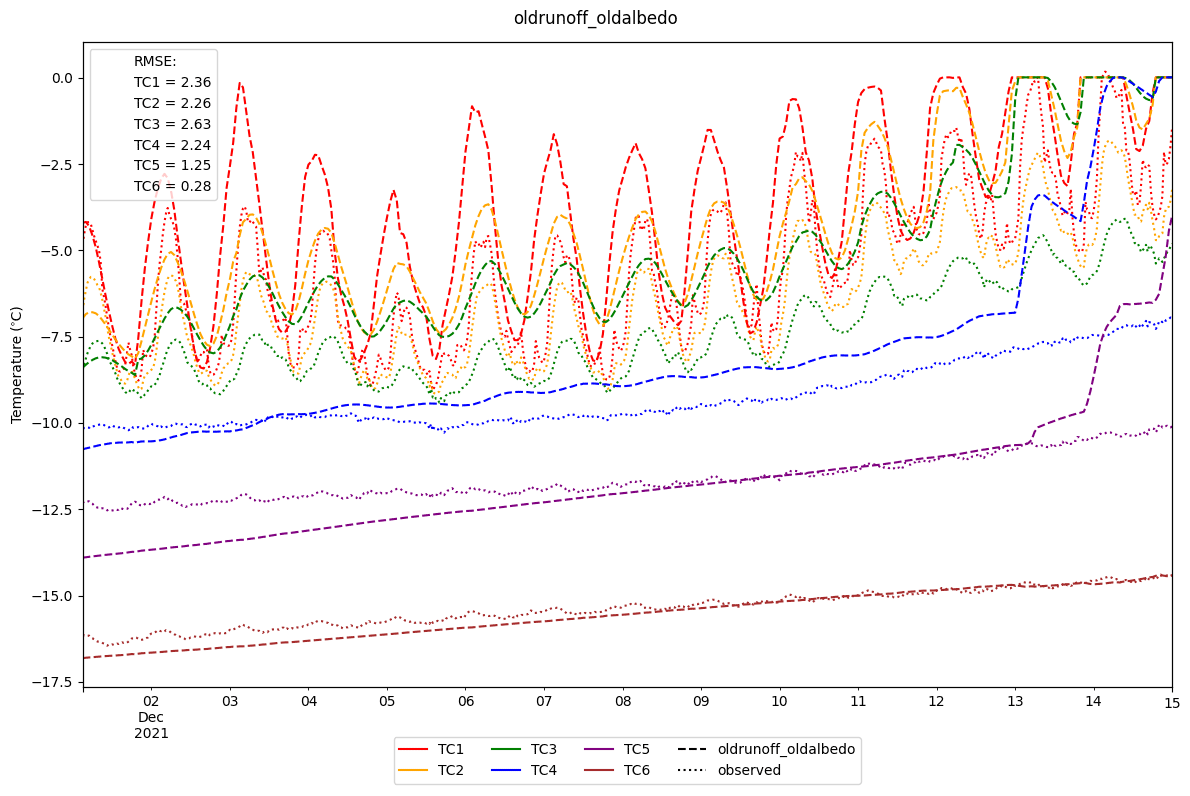
Figure A1Modelled internal ice temperatures from oldrunoff_oldalbedo over the first 2 weeks of December. Thermocouples were initially deployed at six different depths: 0.05, 0.1, 0.2, 0.5, 1.0 and 2.0 m. Note that the measurements are not at a constant depth with time as the sensors were melting out over the period.
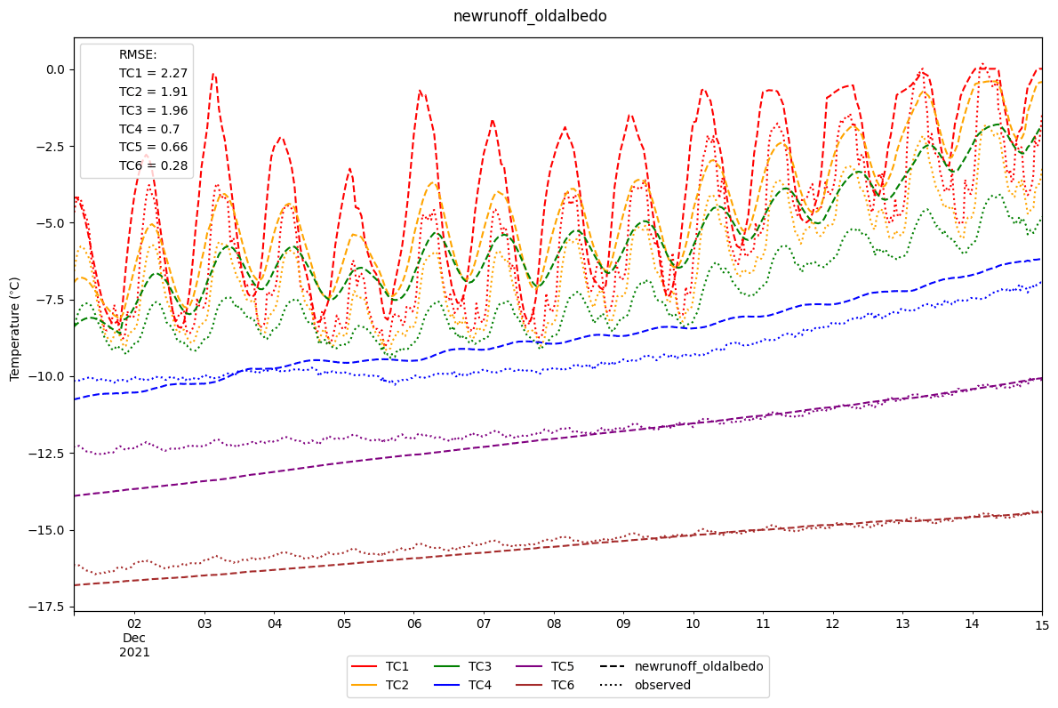
Figure A2Modelled internal ice temperatures from newrunoff_oldalbedo over the first 2 weeks of December. Thermocouples were initially deployed at six different depths: 0.05, 0.1, 0.2, 0.5, 1.0 and 2.0 m. Note that the measurements are not at a constant depth with time as the sensors were melting out over the period.
The data and model configuration are available in Pletzer (2024, https://doi.org/10.5281/zenodo.10565032).
TP, JPC, NJC and MK designed the study. TP and JPC devised the methodology. TP implemented and modified WRF-Hydro/Glacier, collected CWG AWS data and produced the results. TE provided expert advice on the WRF-Hydro/Glacier model. TP, JPC and NJC contributed to the analysis. TP wrote the manuscript with edits from the co-authors. MK provided funding for the field work.
The contact author has declared that none of the authors has any competing interests.
Publisher’s note: Copernicus Publications remains neutral with regard to jurisdictional claims made in the text, published maps, institutional affiliations, or any other geographical representation in this paper. While Copernicus Publications makes every effort to include appropriate place names, the final responsibility lies with the authors.
The authors wish to acknowledge the use of New Zealand eScience Infrastructure (NeSI) high-performance computing facilities and consulting support as part of this research. New Zealand's national facilities are provided by NeSI and funded jointly by NeSI's collaborator institutions and through the Ministry of Business, Innovation and Employment's Research Infrastructure programme.
This research has been supported by the Antarctic Science Platform (grant no. ANTA1801) and the Royal Society of New Zealand (grant no. RDF-UOC1701). The University of Otago provided funding for this research.
This paper was edited by Daniel Viviroli and reviewed by two anonymous referees.
Bergstrom, A., Gooseff, M. N., Myers, M., Doran, P. T., and Cross, J. M.: The seasonal evolution of albedo across glaciers and the surrounding landscape of Taylor Valley, Antarctica, The Cryosphere, 14, 769–788, https://doi.org/10.5194/tc-14-769-2020, 2020. a, b, c, d
Bergstrom, A., Gooseff, M., Fountain, A., and Hoffman, M.: Long-term shifts in feedbacks among glacier surface change, melt generation and runoff, McMurdo Dry Valleys, Antarctica, Hydrol. Process., 35, e14292, https://doi.org/10.1002/hyp.14292, 2021. a
Brandt, R. E. and Warren, S. G.: Solar-heating rates and temperature profiles in Antarctic snow and ice, J. Glaciol., 39, 99–110, https://doi.org/10.3189/S0022143000015756, 1993. a
Brun, E., Martin, E., Simon, V., Gendre, C., and Coleou, C.: An Energy and Mass Model of Snow Cover Suitable for Operational Avalanche Forecasting, J. Glaciol., 35, 333–342, https://doi.org/10.3189/s0022143000009254, 1989. a
Brun, E., David, P., Sudul, M., and Brunot, G.: A numerical model to simulate snow-cover stratigraphy for operational avalanche forecasting, J. Glaciol., 38, 13–22, https://doi.org/10.3189/s0022143000009552, 1992. a, b
Brun, E., Six, D., Picard, G., Vionnet, V., Arnaud, L., Bazile, E., Boone, A., Bouchard, A., Genthon, C., Guidard, V., Le Moigne, P., Rabier, F., and Seity, Y.: Snow/atmosphere coupled simulation at Dome C, Antarctica, J. Glaciol., 57, 721–736, https://doi.org/10.3189/002214311797409794, 2011. a
Cross, J. M., Fountain, A. G., Hoffman, M. J., and Obryk, M. K.: Physical Controls on the Hydrology of Perennially Ice-Covered Lakes, Taylor Valley, Antarctica (1996–2013), J. Geophys. Res.-Earth, 127, e2022JF006833, https://doi.org/10.1029/2022JF006833, 2022. a, b, c
Dadic, R., Mullen, P. C., Schneebeli, M., Brandt, R. E., and Warren, S. G.: Effects of bubbles, cracks, and volcanic tephra on the spectral albedo of bare ice near the Transantarctic Mountains: Implications for sea glaciers on Snowball Earth, J. Geophys. Res.-Earth, 118, 1658–1676, https://doi.org/10.1002/jgrf.20098, 2013. a, b, c, d, e, f
Doran, P. and Fountain, A.: High frequency measurements from Commonwealth Glacier Meteorological Station (COHM), McMurdo Dry Valleys, Antarctica (1993–2021, ongoing), https://doi.org/10.6073/pasta/1fd2035c9efea9f105ecb1d 6212448cc, 2022. a, b
Eidhammer, T., Booth, A., Decker, S., Li, L., Barlage, M., Gochis, D., Rasmussen, R., Melvold, K., Nesje, A., and Sobolowski, S.: Mass balance and hydrological modeling of the Hardangerjøkulen ice cap in south-central Norway, Hydrol. Earth Syst. Sci., 25, 4275–4297, https://doi.org/10.5194/hess-25-4275-2021, 2021. a, b, c, d, e, f, g, h, i, j
Fitzsimons, S. J.: Formation of thrust-block moraines at the margins of dry-based glaciers, south Victoria Land, Antarctica, Ann. Glaciol., 22, 68–74, https://doi.org/10.3189/1996aog22-1-68-74, 1996. a
Fountain, A. G. and Doran, P. T.: Climatology of katabatic winds in the McMurdo dry valleys, southern Victoria Land, Antarctica, J. Geophys. Res., 109, 3114, https://doi.org/10.1029/2003JD003937, 2004. a
Fountain, A. G., Dana, G. L., Lewis, K. J., Vaughn, B. H., and Mcknight, D. H.: Glaciers of the Mcmurdo Dry Valleys, Southern Victoria Land, Antarctica, 65–75, https://doi.org/10.1029/ar072p0065, 1998. a, b
Fountain, A. G., Nylen, T. H., Monaghan, A., Basagic, H. J., and Bromwich, D.: Snow in the Mcmurdo Dry Valleys, Antarctica, Int. J. Climatol., 30, 633–642, https://doi.org/10.1002/joc.1933, 2010. a, b, c, d
Fountain, A. G., Basagic, H. J., and Niebuhr, S.: Glaciers in equilibrium, McMurdo Dry Valleys, Antarctica, J. Glaciol., 62, 976–989, https://doi.org/10.1017/jog.2016.86, 2016. a
Gerbaux, M., Genthon, C., Etchevers, P., Vincent, C., and Dedieu, J. P.: Surface mass balance of glaciers in the French Alps: Distributed modeling and sensitivity to climate change, J. Glaciol., 51, 561–572, https://doi.org/10.3189/172756505781829133, 2005. a
Gillett, S. and Cullen, N. J.: Atmospheric controls on summer ablation over Brewster Glacier, New Zealand, Int. J. Climatol., 31, 2033–2048, https://doi.org/10.1002/JOC.2216, 2011. a
Gochis, D. J., Barlage, M., Cabell, R., Casali, M., Dugger, A., Fitzgerald, K., Mcallister, M., Mccreight, J., Rafieeinasab, A., Read, L., Sampson, K., Yates, D., and Zhang, Y.: The NCAR WRF-Hydro® Modeling System Technical Description v5.1.1, Tech. rep., NCAR, https://ral.ucar.edu/projects/wrf_hydro/documentation/wrf-hydro-v511-documentation (last access: 24 January 2024), 2020. a, b
Gooseff, M. and Mcknight, D.: Seasonal high-frequency measurements of discharge, water temperature, and specific conductivity from Lost Seal Stream at F3, McMurdo Dry Valleys, Antarctica (1993–2020, ongoing), EDI Data Portal [data set], https://doi.org/10.6073/pasta/982b027e0ed7a1854c22 de1396348362, 2021. a, b, c
Gooseff, M. N., McKnight, D. M., Doran, P., Fountain, A. G., and Lyons, W. B.: Hydrological connectivity of the landscape of the McMurdo Dry Valleys, Antarctica, Geography Compass, 5, 666–681, https://doi.org/10.1111/j.1749-8198.2011.00445.x, 2011. a, b, c, d
Gooseff, M. N., Wlostowski, A., McKnight, D. M., and Jaros, C.: Hydrologic connectivity and implications for ecosystem processes – Lessons from naked watersheds, Geomorphology, 277, 63–71, https://doi.org/10.1016/j.geomorph.2016.04.024, 2017. a
Gooseff, M. N., McKnight, D. M., Doran, P. T., and Fountain, A.: Long-term stream hydrology and meteorology of a Polar Desert, the McMurdo Dry Valleys, Antarctica, Hydrol. Process., 36, e14623, https://doi.org/10.1002/hyp.14623, 2022. a
Hoffman, M.: Spatial and Temporal Variability of Glacier Melt in Spatial and Temporal Variability of Glacier Melt in the McMurdo Dry Valleys, Antarctica the McMurdo Dry Valleys, Antarctica, Ph.D. thesis, Portland State University, Portland, https://doi.org/10.15760/etd.744, 2011. a, b, c, d, e, f, g, h, i
Hoffman, M. J., Fountain, A. G., and Liston, G. E.: Surface energy balance and melt thresholds over 11 years at Taylor Glacier, Antarctica, J. Geophys. Res.-Earth, 113, F04014, https://doi.org/10.1029/2008JF001029, 2008. a
Hoffman, M. J., Fountain, A. G., and Liston, G. E.: Near-surface internal melting: A substantial mass loss on Antarctic Dry Valley glaciers, J. Glaciol., 60, 361–374, https://doi.org/10.3189/2014JoG13J095, 2014. a, b, c, d, e, f, g
Hofsteenge, M. G., Cullen, N. J., Reijmer, C. H., van den Broeke, M., Katurji, M., and Orwin, J. F.: The surface energy balance during foehn events at Joyce Glacier, McMurdo Dry Valleys, Antarctica, The Cryosphere, 16, 5041–5059, https://doi.org/10.5194/tc-16-5041-2022, 2022. a, b
Hofsteenge, M. G., Cullen, N. J., Reijmer, C. H., Van Den Broeke, M., and Katurji, M.: Meteorological drivers of melt for two nearby glaciers in the McMurdo Dry Valleys of Antarctica, J. Glaciol., 98, 1–13, https://doi.org/10.1017/jog.2023.98, 2023. a
Kerandi, N., Arnault, J., Laux, P., Wagner, S., Kitheka, J., and Kunstmann, H.: Joint atmospheric-terrestrial water balances for East Africa: a WRF-Hydro case study for the upper Tana River basin, Theor. Appl. Climatol., 131, 1337–1355, https://doi.org/10.1007/s00704-017-2050-8, 2018. a
Kirchner, J. W.: Getting the right answers for the right reasons: Linking measurements, analyses, and models to advance the science of hydrology, Water Resour. Res., 42, W03S04, https://doi.org/10.1029/2005WR004362, 2006. a
Lahmers, T., Kumar, S., Dugger, A., Gochis, D., and Santanello, J.: Impacts of wildfires on the 2020 floods in southeast Australia: A vegetation data-assimilation case study using the NASA coupled LIS/WRF-Hydro system, EGU General Assembly 2021, online, 19–30 Apr 2021, EGU21-9006, https://doi.org/10.5194/egusphere-egu21-9006, 2021. a
Lee, J. R., Raymond, B., Bracegirdle, T. J., Chadès, I., Fuller, R. A., Shaw, J. D., and Terauds, A.: Climate change drives expansion of Antarctic ice-free habitat, Nature, 547, 49–54, https://doi.org/10.1038/nature22996, 2017. a
Li, L., Gochis, D. J., Sobolowski, S., and Mesquita, M. D.: Evaluating the present annual water budget of a Himalayan headwater river basin using a high-resolution atmosphere-hydrology model, J. Geophys. Res., 122, 4786–4807, https://doi.org/10.1002/2016JD026279, 2017. a
MacDonell, S.: Meltwater generation and drainage system on an Antarctic cold-based glacier, Ph.D. thesis, University of Otago, Dunedin, 2008. a, b, c
Macdonell, S. A., Fitzsimons, S. J., and Mölg, T.: Seasonal sediment fluxes forcing supraglacial melting on the Wright Lower Glacier, McMurdo Dry Valleys, Antarctica, Hydrol. Process., 27, 3192–3207, https://doi.org/10.1002/hyp.9444, 2013. a, b
Myers, M. E., Doran, P. T., and Myers, K. F.: Valley-floor snowfall in Taylor Valley, Antarctica, from 1995 to 2017: Spring, summer and autumn, Antarct. Sci., 34, 325–335, https://doi.org/10.1017/S0954102022000256, 2022. a
Nylen, T. H., Fountain, A. G., and Doran, P. T.: Climatology of katabatic winds in the McMurdo dry valleys, southern Victoria Land, Antarctica, J. Geophys. Res.-Atmos., 109, D03114, https://doi.org/10.1029/2003JD003937, 2004. a
Obryk, M. K., Doran, P. T., Fountain, A. G., Myers, M., and McKay, C. P.: Climate From the McMurdo Dry Valleys, Antarctica, 1986–2017: Surface Air Temperature Trends and Redefined Summer Season, J. Geophys. Res.-Atmos., 125, e2019JD032180, https://doi.org/10.1029/2019JD032180, 2020. a, b
Pal, S., Dominguez, F., Dillon, M. E., Alvarez, J., Garcia, C. M., Nesbitt, S. W., and Gochis, D.: Hydrometeorological Observations and Modeling of an Extreme Rainfall Event Using WRF and WRF-Hydro during the RELAMPAGO Field Campaign in Argentina, J. Hydrometeorol., 22, 331–351, https://doi.org/10.1175/JHM-D-20-0133.1, 2021. a
Pletzer, T.: Model configuration and data used in “The application and modification of WRF-Hydro/Glacier to a cold-based Antarctic glacier”, Zenodo [data set], https://doi.org/10.5281/zenodo.10565032, 2024.
Reijmer, C. H., Bintanja, R., and Greuell, W.: Surface albedo measurements over snow and blue ice in thematic mapper bands 2 and 4 in Dronning Maud Land, Antarctica, J. Geophys. Res.-Atmos., 106, 9661–9672, https://doi.org/10.1029/2000JD900718, 2001. a
Senatore, A., Mendicino, G., Gochis, D. J., Yu, W., Yates, D. N., and Kunstmann, H.: Fully coupled atmosphere-hydrology simulations for the central Mediterranean: Impact of enhanced hydrological parameterization for short and long time scales, J. Adv. Model. Earth Sy., 7, 1693–1715, https://doi.org/10.1002/2015MS000510, 2015. a
Shafqat Mehboob, M., Kim, Y., Lee, J., and Eidhammer, T.: Quantifying the sources of uncertainty for hydrological predictions with WRF-Hydro over the snow-covered region in the Upper Indus Basin, Pakistan, J. Hydrol., 614, 128500, https://doi.org/10.1016/j.jhydrol.2022.128500, 2022. a
Singley, J. G., Gooseff, M. N., McKnight, D. M., and Hinckley, E. S.: The Role of Hyporheic Connectivity in Determining Nitrogen Availability: Insights From an Intermittent Antarctic Stream, J. Geophys. Res.-Biogeo., 126, e2021JG006309, https://doi.org/10.1029/2021JG006309, 2021. a
Speirs, J. C., Steinhoff, D. F., McGowan, H. A., Bromwich, D. H., and Monaghan, A. J.: Foehn winds in the McMurdo Dry Valleys, Antarctica: The origin of extreme warming events, J. Climate, 23, 3577–3598, https://doi.org/10.1175/2010JCLI3382.1, 2010. a
Steinhoff, D. F., Bromwich, D. H., and Monaghan, A.: Dynamics of the foehn mechanism in the Mcmurdo Dry Valleys of Antarctica from polar WRF, Q. J. Roy. Meteor. Soc., 139, 1615–1631, https://doi.org/10.1002/qj.2038, 2013. a
Van Den Broeke, M., Van As, D., and Reijmer, C.: Assessing and Improving the Quality of Unattended Radiation Observations in Antarctica, J. Atmos. Ocean. Tech., 21, 1417–1431, 2004. a
Vionnet, V., Brun, E., Morin, S., Boone, A., Faroux, S., Le Moigne, P., Martin, E., and Willemet, J.-M.: The detailed snowpack scheme Crocus and its implementation in SURFEX v7.2, Geosci. Model Dev., 5, 773–791, https://doi.org/10.5194/gmd-5-773-2012, 2012. a, b, c
Warren, S. G.: Optical properties of snow, Rev. Geophys., 20, 67–89, https://doi.org/10.1029/RG020i001p00067, 1982. a, b, c
Xiang, T., Vivoni, E. R., Gochis, D. J., and Mascaro, G.: On the diurnal cycle of surface energy fluxes in the North American monsoon region using the WRF-Hydro modeling system, J. Geophys. Res.-Atmos., 122, 9024–9049, https://doi.org/10.1002/2017JD026472, 2017. a
- Abstract
- Introduction
- Model description
- Methods and data
- Modifications
- Model comparison and evaluation
- Future research and outlook
- Appendix A: Internal ice temperatures from oldrunoff_oldalbedo and newrunoff_oldalbedo
- Code and data availability
- Author contributions
- Competing interests
- Disclaimer
- Acknowledgements
- Financial support
- Review statement
- References