Catchment response to climatic variability: implications for root zone storage and streamflow predictions

This paper investigates the influence of multi-decadal climatic variability on the temporal evolution of root zone storage capacities (S_r,max) and its implications for streamflow predictions in the Meuse basin. Through a comprehensive analysis of 286 catchments across Europe and the US that are hydro-climatically comparable to the Meuse basin, we construct inter-decadal distributions of past deviations in evaporative ratios (I_E) from expected values based on catchment aridity (I_A). These distributions of ΔI_E were then used to estimate inter-decadal changes in S_r,max and to quantify the associated consequences for streamflow predictions in the Meuse basin. Our findings reveal that, while catchments do not strictly adhere to their specific parametric Budyko curves over time, the deviations in I_E are generally very minor, with an average ΔI_E=0.01 and an interquartile range (IQR) of −0.01 to 0.03. Consequently, these minor deviations lead to limited inter-decadal changes in S_r,max, mostly ranging between −10 and +21 mm (−5 % to +10 %). When these changes (ΔS_r,max) are accounted for in hydrological models, the impact on streamflow predictions in the Meuse basin is found to be marginal, with the most significant shifts in monthly evaporation and streamflow not exceeding 4 % and 12 %, respectively. Our study underscores the utility of parametric Budyko-style equations for first-order estimates of future S_r,max in hydrological models, even in the face of climate change and variability. This research contributes to a more nuanced understanding of hydrological responses to changing climatic conditions and offers valuable insights for future climate impact studies in hydrology.

1 Introduction

Transpiration from vegetation is, on average, the largest water flux that leaves terrestrial hydrological systems (Jasechko, 2018). In spite of some uncertainty (Coenders-Gerrits et al., 2014), its magnitude is controlled by the interplay between sub-surface water supply and canopy water demand (Eagleson, 1982; Milly, 1994; Rodriguez-Iturbe et al., 2007; Donohue et al., 2007; Jaramillo et al., 2018). Both individual plants and the composition of plant communities within given spatial domains (hereafter referred to as vegetation for brevity) have, over time, adapted to local environmental and hydro-climatic conditions to ensure continuous and sufficient access to water, nutrients, and light, which has allowed their survival (Yuan et al., 2019; Ma et al., 2021). Adaptation strategies include, amongst others, the regulation of water use efficiency (e.g. Troch et al., 2009; Flo et al., 2021) or the adaptation of the extent of root systems so that roots penetrate large-enough sub-surface pore volumes for water supply to satisfy transpiration demand during dry periods (e.g. Gao et al., 2014; Fan et al., 2017). This sub-surface pore volume between field capacity and permanent wilting point defines the maximum water volume that is within the reach of roots and that is thus available for plant transpiration, hereafter referred to as root zone storage capacity S_r,max (mm). Indeed, S_r,max is a core property of terrestrial hydrological systems as it regulates, to a large extent, the partitioning of water fluxes into drainage of liquid water and, thus, eventually, streamflow Q (mm d⁻¹), vapour released to the atmosphere as transpiration E_T (mm d⁻¹), and interception or soil evaporation E_I (mm d⁻¹) (Savenije and Hrachowitz, 2017).

At the catchment scale, S_r,max has, in the past, been quantified with three methods: firstly, by calibration as parameter of hydrological models (e.g. Fenicia et al., 2009; Coxon et al., 2020; Fowler et al., 2020; Bouaziz et al., 2021; Hanus et al., 2021; Wang et al., 2023); secondly, as product of estimates of average root depth, soil porosity, and water content at field capacity (e.g. Clark et al., 2008; Maxwell et al., 2015); and, thirdly, by following optimality principles and thus maximising variables such as net primary production, transpiration rates, or others (e.g. Kleidon, 2004; Guswa, 2008; Sivandran and Bras, 2012; Speich et al., 2020). Although all three methods mentioned above are correct in principle, insufficient data often limits their use. For example, although there are observations of root depth for several thousand individual plants worldwide (Guerrero-Ramírez et al., 2021), it is difficult to meaningfully upscale these values to plant communities with different compositions, ages, or densities. In addition, these estimates are mostly snapshots in time reflecting past conditions and, similarly to the calibration method, do not give any indication of the potential future evolution of S_r,max.

Alternatively, there is increasing evidence that S_r,max can be robustly estimated exclusively based on water balance data, i.e. long-term estimates of precipitation P (mm d⁻¹) and actual evaporation $E_{\mathrm{A}}=E_{\mathrm{T}}+E_{\mathrm{I}}$ (e.g. Donohue et al., 2012; Gentine et al., 2012; Gao et al., 2014, 2016; de Boer-Euser et al., 2016; Wang-Erlandsson et al., 2016; Dralle et al., 2021; Hrachowitz et al., 2021; McCormick et al., 2021; van Oorschot et al., 2021; Stocker et al., 2023). Under the assumption that vegetation allocates resources in an efficient way between above- and sub-surface growth (Guswa, 2008; Schymanski et al., 2008), root systems and, thus, S_r,max will not be larger than necessary to guarantee access to sufficient water during dry periods with certain return periods. The water of volume that, in the past, has been transpired during the driest periods and that can be estimated via the water balance must have been accessible to roots and therefore must reflect the magnitude of the water volume that was stored in the sub-surface and that was accessible to plants during these dry periods, i.e. S_r,max.

This approach offers the advantage that an evolution of S_r,max over time, either through natural adaptation to changing hydro-climatic conditions (e.g. Jaramillo et al., 2018) or through human interventions such as deforestation (e.g. Nijzink et al., 2016a; Hrachowitz et al., 2021) and irrigation (van Oorschot et al., 2024), is manifest in changes in dry-period transpiration E_T. This offers an opportunity not only to trace the past evolution of S_r,max over time but also, together with projections of future hydro-climatic conditions, including P and E_P, to quantify its potential future trajectories and the associated effects of this temporal evolution of S_r,max with regard to the hydrological response.

More specifically, estimating S_r,max from the water balance requires knowledge of E_A. For past conditions, this can be robustly estimated from the water balance by assuming negligible storage change, i.e. $\mathrm{d}S/\mathrm{d}t\sim \mathrm{0}$, which is satisfied for the vast majority of catchments worldwide over timescales of around 10 years (Han et al., 2020). Climate model projections can generate, in addition to estimates of future P and potential evaporation E_P (mm d⁻¹), estimates of future E_A. However, the latter are subject to major uncertainties (e.g. van Oorschot et al., 2021). As an alternative method, non-parametric formulations of the Budyko hypothesis demonstrate that the long-term partitioning of water fluxes – expressed as the evaporative index $I_{\mathrm{E}}=E_{\mathrm{A}}/P=\mathrm{1}-Q/P$ (–) – and, thus, of the hydrological response of catchments globally is, to the first order, controlled by the aridity index $I_{\mathrm{A}}=E_{\mathrm{P}}/P$ (Schreiber, 1904; Oldekop, 1911; Budyko and Miller, 1974). To reduce the scatter around these non-parametric Budyko-style curves and to assign catchments a unique position in the I_A–I_E space, parametric re-formulations such as the Tixeront–Fu equation (Tixeront, 1964; Fu, 1981; Zhang et al., 2004) and similar expressions (see Andréassian et al., 2016) were developed:

$$\begin{array}{}\text{(1)}& {\displaystyle \frac{E_{\mathrm{A}}}{P}}=\mathrm{1}+{\displaystyle \frac{E_{\mathrm{P}}}{P}}-{\left[\mathrm{1}+{\left({\displaystyle \frac{E_{\mathrm{P}}}{P}}\right)}^{\mathit{\omega }}\right]}^{\frac{\mathrm{1}}{\mathit{\varpi }}},\end{array}$$

where ω (–) [1, ∞) is a catchment-specific effective parameter that aggregates all other influences on I_E next to I_A (Berghuijs and Woods, 2016). Higher values of ω indicate higher $E_{\mathrm{A}}/P$.

As this relationship has emerged from catchment responses and, thus, also vegetation, having adapted to past hydro-climatic conditions, expressed by I_A, it is plausible to assume that the hydrological partitioning I_E of a catchment will eventually adapt to a changing future I_A in a corresponding way by moving along its catchment-specific curve defined by ω. This reasoning then allows us to estimate future E_A based on future projections of P and E_P (Roderick and Farquhar, 2011; Wang et al., 2016; Liu et al., 2020). As a consequence, the effects of a changing future E_A on the future root zone storage capacity S_r,max can be quantified. In contrast to the vast majority of climate impact studies, which, in the absence of further information, assume time-invariant S_r,max even under changing future climate (e.g. Prudhomme et al., 2014; Brunner et al., 2019; Hakala et al., 2020; Rottler et al., 2021; Hanus et al., 2021), the use of such a time-variant formulation of S_r,max as parameter in hydrological models has the potential to provide more reliable predictions of the future hydrological response of catchments, as, for example, demonstrated in a recent proof-of-concept study by Bouaziz et al. (2022) for the Meuse basin in northwestern Europe. They found with model simulations that the adaptation of S_r,max to future climate conditions, expressed as I_A, can cause major shifts in seasonal water supply. This involved future increases in S_r,max and, thus, increases in vegetation-accessible sub-surface water volumes, which lead to increases in summer E_A of up to 15 %; these, in turn, reduced groundwater recharge, which resulted in 10 % decreases in late-summer and autumn groundwater storage, eventually causing winter flows that could be up to 20 % lower as compared to model runs that used constant values of S_r,max estimated from past hydro-climatic conditions. These findings are qualitatively consistent with the results of Speich et al. (2020), who reported significant changes in modelled streamflow when replacing a static parameter used to describe S_r,max with a forest dynamics model. More generally, Wagener et al. (2003) and Merz et al. (2011) documented the role of time-variant model parameters, including S_r,max (in their papers referred to as root constant and FC, respectively), by comparing model calibrations over multiple time windows. In a different approach, the importance of time-variable vegetation dynamics was demonstrated by Duethmann et al. (2020), who used remotely sensed vegetation indices, including the normalised difference vegetation index (NDVI), to account for temporal variations in evaporation surface resistance in the Penman equation, leading to considerably improved model skill with regard to reproducing observed river flow over multiple decades.

A major assumption underlying the approach of Bouaziz et al. (2022) is that, under changing future conditions, catchments will indeed follow their specific Budyko curve as defined by the time-invariant parameter ω, which describes the long-term average past conditions. The resulting I_E is, in the following, referred to as the expected I_E,exp. Several recent studies have pointed out that this assumption may not strictly hold and that ω itself may be subject to fluctuations over time (e.g. Berghuijs and Woods, 2016; Reaver et al., 2022). While of minor relevance to humid environments, I_E and, thus, E_A become proportionally more sensitive to fluctuations in ω with increasing aridity I_A (Gudmundsson et al., 2016). As a consequence, it has to be expected that estimates of future E_A and the associated S_r,max are subject to uncertainties or deviations ΔI_E,exp from I_E,exp that are not accounted for by Bouaziz et al. (2022).

The overall objectives of this paper are thus (1) to quantify the deviations in I_E following changes in I_A based on historical observations and (2) to analyse how this has, in the past, propagated further into uncertainties in time-variant estimates of S_r,max in contrasting environments over multiple decades in a large-sample approach using long-term water balance data from 286 catchments from Great Britain (GB), the US, and the Meuse basin. In a direct follow up to Bouaziz et al. (2022), who modelled the impact of a changing future climate on the hydrological response in several catchments of the Meuse basin without accounting for deviations in I_E and, thus, uncertainties in S_r,max, we will, in a third step, using the same model, (3) quantify the additional effect of deviations in I_E and, thus, uncertainties in S_r,max on the hydrological response in the Meuse basin and compare it to previous streamflow predictions in the Meuse basin (Bouaziz et al., 2022) that do not account for these uncertainties. Specifically, we will test the hypothesis that the inter-decadal evolution of S_r,max, reflecting vegetation adaptation to factors other than I_A, which is manifest in deviations from the expected future I_E,exp and thus from the associated future S_r,max, lead to significant changes in the predicted future hydrological response in the Meuse basin and needs to be accounted for in hydrological climate impact studies.

2 Study area and data

2.1 Study area

The hydrological model experiment in this study is done for the Meuse River basin upstream of Borgharen at the border between Belgium and the Netherlands (Fig. 1), which spans an area of 21 300 km² in northwestern Europe. Largely located in the Ardennes, a rolling-hill landscape characterised by ridges and incised valleys, the elevation reaches up to around 650 m. Approximately 60 % of the basin is used for agriculture, while 30 % is covered by forests (Bouaziz et al., 2022).

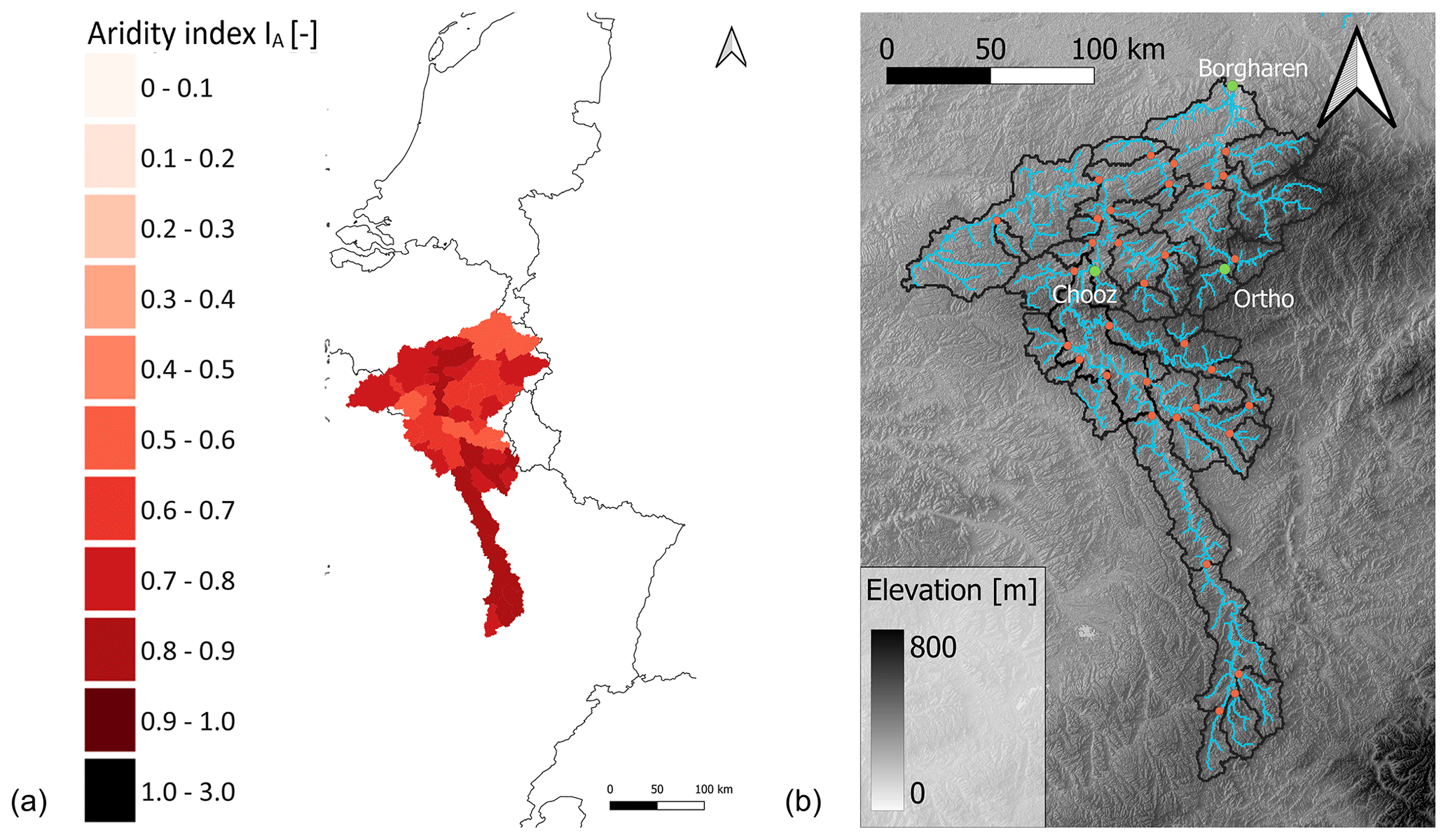
Figure 1 (a) The location of the Meuse basin in northwestern Europe, where the red colour indicates the aridity index I_A of the catchment; (b) the elevation range, river trajectory, and gauges in the Meuse River basin. Gauges are indicated with orange dots. The catchments of Borgharen, Ortho, and Chooz are specifically highlighted (with green) as they are separately emphasised in some of the results and analyses.

The Meuse basin is characterised by a temperate humid climate with average annual precipitation of around 920 mm yr⁻¹, potential evaporation of around 610 mm yr⁻¹, and streamflow of around 400 mm yr⁻¹. The Meuse is a rain-fed river with a response time of several hours up to a few days. Transient snowpacks can be present for a few days in some parts of the basin but are overall of minor importance (Bouaziz et al., 2021). The streamflow has strong seasonality, with low summer flows and high winter flows, which are, on average, 4 times higher than the summer flow (De Wit et al., 2007). Precipitation falls relatively homogenously throughout the year, and the seasonality of the streamflow is thus mainly caused by the seasonal differences in solar-energy input and, thus, evaporation.

2.2 Data

To quantify the deviations ΔI_E,exp from expected I_E,exp, we adopted a large-sample strategy using long-term water balance data from catchments in contrasting environments.

Table 1 Segmentation of data by 10-year periods, with the exception of the CAMELS USA, which has two periods of 9 years. Note the extra time period for the France Meuse data in comparison with the Belgium and Netherlands data.

For the Meuse river basin, daily precipitation, temperature, and radiation were obtained for the 1989–2018 period from the E-OBS v20.0 data set (Cornes et al., 2018) and were pre-processed as described by Bouaziz et al. (2022). Temperature was downscaled using a digital elevation model and a fixed temperature lapse rate, while potential evaporation was estimated using the Makkink method (Hooghart and Lablans, 1988). This method was chosen to balance the availability of the required data with their suitability for hydrological model applications (Oudin et al., 2005). Monthly bias correction was applied to address underestimation of precipitation. Daily streamflow data were available for 23 catchments within the Meuse basin from water authorities in Belgium (Service publique de Wallonie), France (Eau France), and the Netherlands (Rijkswaterstaat) for various time periods between 1989–2018 (Table 1). Note that the streamflow data at the station of Borgharen in the Netherlands are constructed by combining observations from the nearby stations St. Pieter on the Meuse and Kanne on the Albert canal (De Wit et al., 2007).

Long-term temporal changes in I_E,exp and deviations ΔI_E,exp therefrom that can be quantified in the Meuse basin remain limited to the 23 catchments that are gauged and streamflow records of 30 years at most. To increase the sample size in space and time and to encompass a broader range of climates, we have, in addition, included data from catchments in GB and the US, available from the CAMELS GB (Coxon et al., 2020) and CAMELS US (Addor et al., 2017) databases for the time periods indicated in Table 1. To ensure consistency, potential evaporation across all data sets was recalculated using the Makkink equation based on mean daily temperature and shortwave radiation (Hooghart and Lablans, 1988). From the full set of 671 catchments available in each of the two CAMELS databases, we excluded from the analysis those that exhibited long-term I_E>I_A, indicating that E_A exceeds E_P and, thus, the energy limit, which is an indicator of major data errors or significant unaccounted water export to adjacent catchments via, for example, groundwater exchange or irrigation water abstraction (Bouaziz et al., 2018). This does not imply that catchments retained for our analysis are not subject to data errors or unaccounted water exports. Although the effect of spurious results cannot be completely avoided, removing catchments which exhibit clear evidence of water balance deficits can at least reduce the impact of spurious effects.

Figure 2 The locations of the catchments that are provided by the large-sample data sets (a) CAMELS GB and (b) CAMELS USA. The red colour indicates the aridity index I_A of the catchment.

Figure 3 Illustration of the long-term average values for the entire period of data analysis.

In addition, catchments were excluded from the analysis if they did not meet the criteria of minimal human impact or if they received more than 10 % of their annual precipitation as snow. The exclusion of catchments with snowfall was necessary due to the temporary water storage capacity of snow, which can lead to inaccurate estimation of root zone storage capacity due to delayed water input (Dralle et al., 2021). This resulted in a total of 286 catchments being used for the subsequent analysis (23 – Meuse basin; 94 – CAMELS GB; 169 – CAMELS USA; Fig. 2), covering a wide range of hydro-climatic conditions, with the catchments in the Meuse basin being located at an intermediate position between the GB and US catchments (Fig. 3). Finally, the data were segmented into distinct 10-year periods (Table 1), allowing us to quantify decadal changes in I_A, I_E, and the associated S_r,max, as well as their decadal deviations from the expected values, i.e. ΔI_E,exp and $\mathrm{\Delta }{S}_{\mathrm{r},\max ,\exp }$.

3 Methods

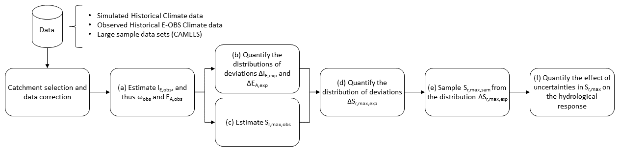
Following the three specific research objectives as formulated in Sect. 1, the experiment of this study is executed in several subsequent steps, shown in Fig. 4: for each of the 286 study catchments, (a) estimate I_E,obs and, thus, ω_obs and E_A,obs from the water balance data of multiple past individual decades in the period 1989–2018 (Sect. 3.1); (b) quantify the distributions of deviations ΔI_E,exp and, thus, ΔE_A,exp from the expected I_E,exp and E_A,exp between subsequent decades (Sect. 3.1); (c) estimate $S_{\mathrm{r},\max ,\mathrm{obs}}$ from the past water balance data and, thus, from E_A,obs of multiple past individual decades (Sect. 3.2); (d) quantify the distribution of deviations $\mathrm{\Delta }{S}_{\mathrm{r},\max ,\exp }$ from the expected $S_{\mathrm{r},\max ,\exp }$ between subsequent decades based on ΔE_A,exp (Sect. 3.2); (e) for the 23 Meuse catchments for the 2009–2018 decade, sample $S_{\mathrm{r},\max ,\mathrm{sam}}$ from the distribution $\mathrm{\Delta }{S}_{\mathrm{r},\max ,\exp }$ (Sect. 3.2); and, finally, (f) quantify the effect of uncertainties in S_r,max on the hydrological response by using the sampled values $S_{\mathrm{r},\max ,\mathrm{sam}}$ as parameters in multiple runs and compare the results to model runs that assume $\mathrm{\Delta }{I}_{\mathrm{E},\exp }=\mathrm{0}$ and, thus, $\mathrm{\Delta }{S}_{\mathrm{r},\max ,\exp }=\mathrm{0}$ (Sect. 3.3).

Figure 4 Overview of the methodological procedure.

3.1 Estimate I_E, E_A, and their deviations from expected values over time

For each of the 286 study catchments, we estimated for each individual decade i with a data record (see Table 1) the decadal average evaporation and the associated decadal average evaporative indices from the observed decadal average balance data:

$$\begin{array}{}\text{(2)}& {\displaystyle }& {\displaystyle }{E}_{\mathrm{A},\mathrm{obs},i}=P_{\mathrm{obs},i}-Q_{\mathrm{obs},i},\text{(3)}& {\displaystyle }& {\displaystyle }{I}_{\mathrm{E},\mathrm{obs},i}=E_{\mathrm{A},\mathrm{obs},i}/P_{\mathrm{obs},i}.\end{array}$$

Together with P_obs,i and $E_{\mathrm{P},\mathrm{obs},i}$, expressed as aridity index $I_{\mathrm{A},\mathrm{obs},i}$, we then use $E_{\mathrm{A},\mathrm{obs},i}$ to solve the parametric Tixeront–Fu formulation of the Budyko hypothesis (Eq. 1) for ω_obs,i for each decade for each individual catchment.

In a next step, assuming that $P_{\mathrm{obs},i+\mathrm{1}}$ and $E_{\mathrm{P},\mathrm{obs},i+\mathrm{1}}$ of the following decade i+1 are projections of an unknown future, we solve Eq. (1) for I_E to “predict” the expected evaporative index of that following decade, i.e. $I_{\mathrm{E},\exp ,i+\mathrm{1}}=E_{\mathrm{A},\exp ,i+\mathrm{1}}/P_{\mathrm{obs},i+\mathrm{1}}$, based on $I_{\mathrm{A},\mathrm{obs},i+\mathrm{1}}$ together with ω_obs,i from the current decade, implying that each catchment will follow its specific curve defined by ω_obs,i. The difference in the expected $I_{\mathrm{E},\exp ,i+\mathrm{1}}$ in relation to the actual observed $I_{\mathrm{E},\mathrm{obs},i+\mathrm{1}}$ then represents the deviation $\mathrm{\Delta }{I}_{\mathrm{E},\exp ,i+\mathrm{1}}$ and, thus, $\mathrm{\Delta }{E}_{\mathrm{A},\exp ,i+\mathrm{1}}$ for that decade i+1 for each individual catchment. The deviations for all decades of all catchments are then aggregated to an individual distribution of deviations for each of the three data sets, i.e. ΔI_E,Meuse, ΔI_E,GB, and ΔI_E,US, and for one distribution of all three data sets combined, i.e. ΔI_E. The general procedure is illustrated in Fig. 5.

Figure 5 The step-by-step process for calculating the error in I_E (ΔI_E) using data with three decades as an example.

3.2 Estimate root zone storage capacity S_r,max and its deviations from expected values over time

For each study catchment and each decade i with a data record we estimated the root zone storage capacity $S_{\mathrm{r},\max ,\mathrm{obs},i}$. This was done on the basis of observed decadal water balance data, as described in detail elsewhere (e.g. Nijzink et al., 2016a; Bouaziz et al., 2020; Hrachowitz et al., 2021).

Briefly, the decadal averages $E_{\mathrm{A},\mathrm{obs},i}$ (Eq. 2) of each study catchment were redistributed to daily values $E_{\mathrm{A},\mathrm{obs},i}\left(t\right)$ by rescaling daily observed values of $E_{\mathrm{P},\mathrm{obs},i}\left(t\right)$ according to the following:

$$\begin{array}{}\text{(4)}& E_{\mathrm{A},\mathrm{obs},i}\left(t\right)={\displaystyle \frac{E_{\mathrm{P},\mathrm{obs},i}\left(t\right)}{E_{\mathrm{P},\mathrm{obs},i}}}{E}_{\mathrm{A},\mathrm{obs},i},\end{array}$$

where t is any given day within a decade i. Note that the rescaling in Eq. (4) is based on the simplifying assumption of a constant $E_{\mathrm{A}}/E_{\mathrm{P}}$ ratio. This does not account for the effects of vegetation water stress and may cause inflated S_r,max estimates in regions with pronounced dry periods (e.g. van Oorschot et al., 2021). The catchments of the Meuse basin for which S_r,max was estimated in this study are characterised by abundant summer precipitation and rather short dry spells. The effect of a constant scaling factor on S_r,max is therefore minor.

These daily estimates of evaporation $E_{\mathrm{A},\mathrm{obs},i}\left(t\right)$ were then used together with daily observed precipitation P_obs,i(t) to compute the time series of daily cumulative storage deficits for a specific year j according to the following:

$$\begin{array}{}\text{(5)}& \begin{array}{rl}& S_{\mathrm{D},j,i}\left(t\right)=\\ & \left\{\begin{array}{ll}\underset{t_{\mathrm{0}}}{\overset{t}{\int }}\left(P_{\mathrm{obs},i}\left(t\right)-E_{\mathrm{A},\mathrm{obs},i}\left(t\right)\right)\mathrm{d}t,& \mathrm{if}\underset{t_{\mathrm{0}}}{\overset{t}{\int }}\left(P_{\mathrm{obs},i}\left(t\right)-E_{\mathrm{A},\mathrm{obs},i}\left(t\right)\right)\mathrm{d}t\le \mathrm{0}\\ \mathrm{0},& \mathrm{if}\underset{t_{\mathrm{0}}}{\overset{t}{\int }}\left(P_{\mathrm{obs},i}\left(t\right)-E_{\mathrm{A},\mathrm{obs},i}\left(t\right)\right)\mathrm{d}t>\mathrm{0}\end{array}\right.\end{array},\end{array}$$

where t₀ is the last preceding day on which the cumulative storage deficit $S_{\mathrm{D},j,i}\left(t\right)=\mathrm{0}$. Note that the effects of interception evaporation E_I on the estimation of storage deficits are negligible, as demonstrated by Bouaziz et al. (2020), and we therefore assumed that E_A=E_T.

The maximum annual storage deficit $S_{\mathrm{D},j,i}$ represents the volume of water that needs to be stored within the reach of roots to provide vegetation with continuous access to water in that year j; this is obtained as follows:

$$\begin{array}{}\text{(6)}& S_{\mathrm{D},j,i}=\max \left(\left|S_{\mathrm{D},j,i}\left(t\right)\right|\right).\end{array}$$

Previous studies suggested that, in a wide spectrum of environments, vegetation develops root systems that allow access to sufficient water to bridge dry spells with return periods of around 20 years (Gao et al., 2014; Nijzink et al., 2016a). The annual storage deficits $S_{\mathrm{D},j,i}$ of all years j in a specific decade i and catchment were therefore used to fit the generalised-extreme-value distribution. This then allowed us to estimate the storage deficit with a 20-year return period, which, here, was defined as the root zone storage capacity for that decade: $S_{\mathrm{r},\max ,\mathrm{obs},i}=S_{\mathrm{D},\mathrm{20}\mathrm{yr},i}$. Note that, strictly seen, S_r,max is a lower limit of the magnitude of vegetation-accessible sub-surface water volumes. Based on Eqs. (2)–(6), it is an estimate of the water volume that was required in the past to meet the estimated E_A (Eq. 2). In principle, the total volume of S_r,max could be higher. However, several previous studies have shown that estimating S_r,max as a parameter of a hydrological model calibrated according to observed streamflow leads to very similar values of S_r,max in many regions worldwide (e.g. Gao et al., 2014; de Boer-Euser et al., 2016; Nijzink et al., 2016a; Hrachowitz et al., 2021; Wang et al., 2024). In other words, this is evidence that models can only reproduce observed streamflow if S_r,max does indeed represent a maximum vegetation-accessible water volume and, thus, an upper limit.

In a next step, assuming that $P_{\mathrm{obs},i+\mathrm{1}}$ of the following decade i+1 is a projection of an unknown future, we follow the same procedure described above by Eqs. (2)–(4) but using $\mathrm{\Delta }{E}_{\mathrm{A},\exp ,i+\mathrm{1}}$ to “predict” the expected root zone storage capacity of the following decade $S_{\mathrm{r},\max ,\exp ,i+\mathrm{1}}$. The difference between the expected $S_{\mathrm{r},\max ,\exp ,i+\mathrm{1}}$ and the actually observed $S_{\mathrm{r},\max ,\mathrm{obs},i+\mathrm{1}}$ then represents the deviation $\mathrm{\Delta }{S}_{\mathrm{R},\max ,\exp ,i+\mathrm{1}}$ for that specific catchment for decade i+1. The deviations for all decades for all catchments are then aggregated to an individual distribution of deviations for each of the three data sets, i.e. $\mathrm{\Delta }{S}_{\mathrm{r},\max ,\mathrm{Meuse}}$, $\mathrm{\Delta }{S}_{\mathrm{r},\max ,\mathrm{GB}}$, and $\mathrm{\Delta }{S}_{\mathrm{r},\max ,\mathrm{US}}$.

3.3 Effect of ΔS_r,max on streamflow

To isolate and quantify the effect of uncertainties ΔS_r,max in predicted S_r,max on predictions of the hydrological response, we run several simulation scenarios with a process-based model for the 23 study catchments in the Meuse basin.

3.3.1 Hydrological model

The hydrological model used in this study is wflow-FLEXTopo (van Verseveld et al., 2024), a fully distributed process-based model designed to represent spatial variability in hydrological processes. The modular model uses flexible model structures for the selection of hydrological response units (HRUs), which are delineated based on topography and land use. See Fig. 6 for a schematic representation of wflow-FLEXTopo within one HRU.

Figure 6 Schematic representation of the wflow-FLEXTopo model for a single-class model including all storages and fluxes (van Verseveld et al., 2024).

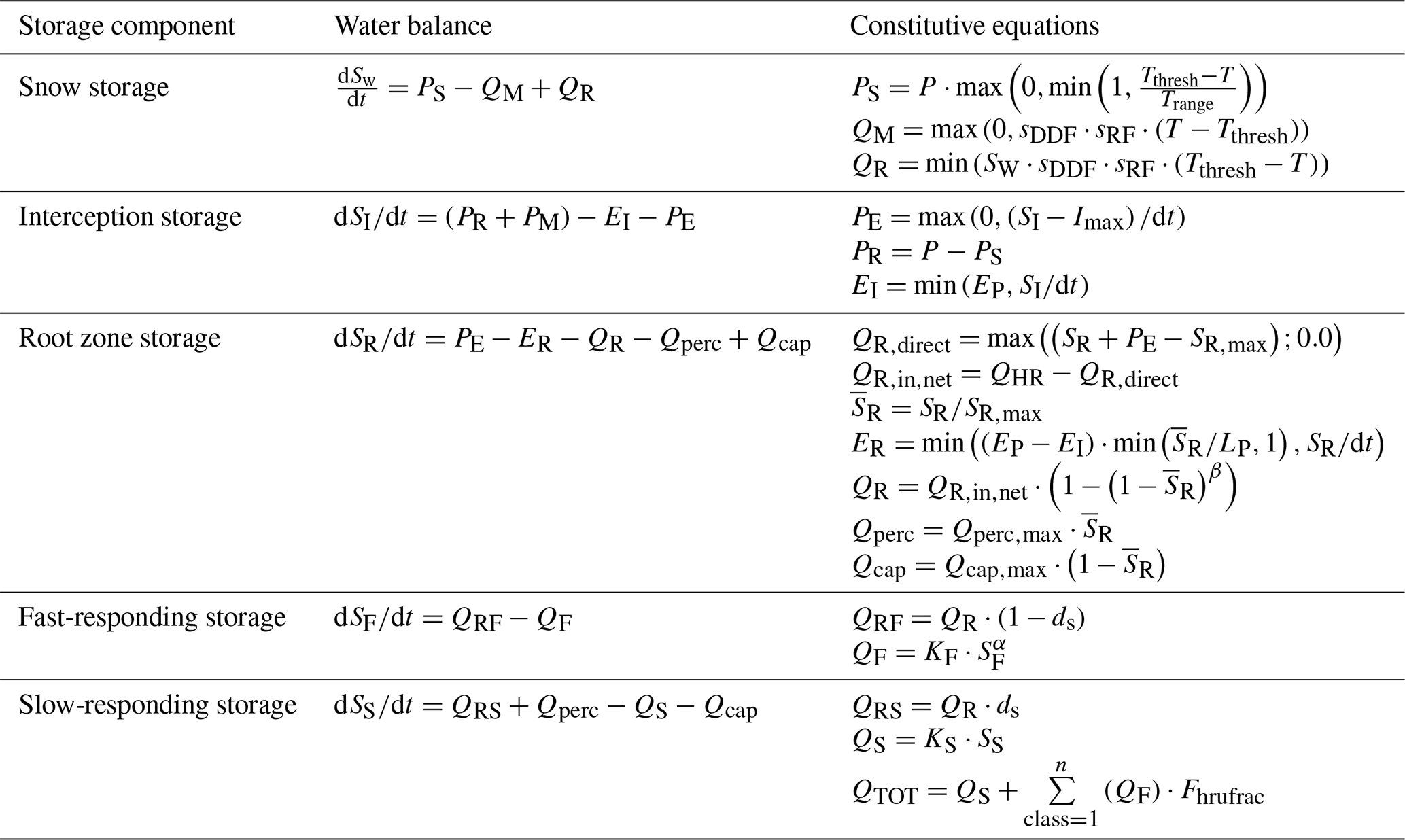
Briefly, each HRU consists of several storage components linked by fluxes, similarly to comparable process-based models successfully used in previous studies (e.g. Fenicia et al., 2006; Euser et al., 2015; Gao et al., 2016; Fowler et al., 2020). Here, we have defined three HRUs that represent wetlands, hillslopes, and plateaus and which are connected through a common groundwater storage (e.g. Hulsman et al., 2021). The HRUs were delineated using the MERIT Hydro data set at 60 m × 90 m resolution (Yamazaki et al., 2019), with a threshold of 5.9 m for the height above the nearest drainage (HAND; Rennó et al., 2008) and a slope threshold of 0.13 following the methodology proposed by Gharari et al. (2011). The hillslopes are associated with forest, and the largest parts of the plateaus are used for crop cultivation agriculture in the study region, as identified using CORINE land cover data (European Environment Agency, 2018). The areal fraction of each of the three HRUs was derived for each cell at a model resolution of approximately 600 m × 900 m, similarly to the sub-grid landscape variability implemented by Nijzink et al. (2016b) in the distributed mesoscale hydrologic model (mHM). All relevant model equations are given in Table 2. Note that Horton ponding and runoff processes (Fig. 6) have minor importance in the study region and were therefore switched off for the model implementation in this study.

Table 2 Water balance and flux equations used in the hydrological model, with variables: P_S is snowfall (mm t⁻¹), Q_M is snowmelt (mm t⁻¹), Q_R is refreezing snow (mm t⁻¹), T_thresh is melting-temperature threshold (°C), T_range is the range over which precipitation partly falls as snow and partly falls as rainfall (°C), T is air temperature (°C), Q_R,pot is potential snowmelt (mm t⁻¹), s_DDF is the degree-day factor (mm t⁻¹ °C), s_RF is a coefficient of refreezing (–), P_R is rainfall (mm t⁻¹), I_max is the maximum interception storage for each class (mm), E_I is interception evaporation (mm t⁻¹), P_E is effective precipitation (mm t⁻¹), L_P is the threshold parameter for water stress (–), F_max is the maximum infiltration capacity (mm t⁻¹), F_dec is the decay coefficient (–), S_R,max is the root zone storage capacity (mm), Q_R,direct is direct runoff (mm t⁻¹), $Q_{\mathrm{R},\mathrm{in},\mathrm{net}}$ is net infiltration in the root zone storage (mm t⁻¹), E_R is the evaporation from the root zone storage (mm t⁻¹), Q_R is runoff (mm t⁻¹), Q_perc is percolation to the slow groundwater (mm t⁻¹), Q_cap is capillary rise from the slow groundwater (mm t⁻¹), Q_perc,max is the maximum percolation parameter (mm t⁻¹), Q_cap,max is the maximum capillary rise flux parameter (mm t⁻¹), Q_RF is inflow in the fast storage (mm t⁻¹), Q_F is fast runoff (mm t⁻¹), K_F is the recession constant (t⁻¹), Q_RS is preferential recharge from the outflow of the root zone storage (mm t⁻¹), Q_S is linear outflow from the slow groundwater storage (mm t⁻¹), K_S is the recession timescale coefficient, Q_TOT is the total streamflow (mm t⁻¹), and F_hrufrac is the fraction of each class in a cell (–).

The model was previously calibrated for, at most, the downstream gauge at Borgharen (Bouaziz et al., 2022) using a multi-objective calibration strategy based on the Nash–Sutcliffe efficiencies of flows (E_NS), as well as on the logarithm of flows (E_NS,log), the Kling–Gupta efficiency of flows (E_KG), and the monthly runoff coefficients as performance metrics (Bouaziz et al., 2022). The model was subsequently evaluated for its skill in reproducing streamflow for all of the other 22 stream gauges in the Meuse basin on the basis of the same performance metrics.

3.3.2 Scenarios

The effect of uncertainties ΔS_r,max in the predicted S_r,max on the predictions of the hydrological response in the 23 study catchments was then quantified by running the calibrated model for the 2009–2018 period and replacing S_r,max with different “predictions” thereof for that period. Following the procedure used to predict S_r,max and ΔS_r,max (Sect. 3.2) from I_E and ΔI_E (Sect. 3.1), we have, for this experiment, used the decadal period 1999–2008 (p₁) as the basis to predict S_r,max and ΔS_r,max for the period 2009–2018 (p₂) in three scenarios.

Baseline scenario ($\mathrm{\Delta }{S}_{\mathrm{r},\max }=\mathrm{0}$)

We estimate ${\mathit{\omega }}_{\mathrm{obs},{\mathrm{p}}_{\mathrm{1}}}$ of the first decade p₁ based on observed data $P_{\mathrm{obs},{\mathrm{p}}_{\mathrm{1}}}$, $E_{\mathrm{P},\mathrm{obs},{\mathrm{p}}_{\mathrm{1}}}$, and $Q_{\mathrm{obs},{\mathrm{p}}_{\mathrm{1}}}$ of that period. Subsequently, we have used these values together with $P_{\mathrm{obs},{\mathrm{p}}_{\mathrm{2}}}$ and $E_{\mathrm{P},\mathrm{obs},{\mathrm{p}}_{\mathrm{2}}}$ of the second decade p₂ to predict the expected $I_{\mathrm{E},\exp ,{\mathrm{p}}_{\mathrm{2}}}$ and, finally, $S_{\mathrm{r},\max ,\exp ,{\mathrm{p}}_{\mathrm{2}}}$ for that second period p₂ in each catchment. The calibrated S_r,max values are then replaced in the model by the predicted values $S_{\mathrm{r},\max ,{\mathrm{p}}_{\mathrm{2}}}$. Re-running the model with $S_{\mathrm{r},\max ,{\mathrm{p}}_{\mathrm{2}}}$ for period p₂ then provides the baseline output of the hydrological response assuming that the catchments follow their specific Budyko curves as defined by their individual ${\mathit{\omega }}_{\mathrm{obs},{\mathrm{p}}_{\mathrm{1}}}$ and that, therefore, $\mathrm{\Delta }{I}_{\mathrm{E},{\mathrm{p}}_{\mathrm{2}}}=\mathrm{0}$ and $\mathrm{\Delta }{S}_{\mathrm{r},\max ,{\mathrm{p}}_{\mathrm{2}}}=\mathrm{0}$. This scenario is equivalent to the approach used by Bouaziz et al. (2022).

Scenario A ($\mathrm{\Delta }{S}_{\mathrm{r},\max }\ne \mathrm{0}$)

The catchments do not follow their specific Budyko curves. In this case, we used the combined distributions of historical deviations ΔI_E from the Meuse, GB, and US data sets to determine $\mathrm{\Delta }{S}_{\mathrm{r},\max ,{\mathrm{p}}_{\mathrm{2}}}$. The predicted $I_{\mathrm{E},\mathrm{pred},{\mathrm{p}}_{\mathrm{2}}}$ for decade p₂ was thus estimated by sampling 100 times from the distribution of deviations ΔI_E and adding the sampled values to the expected value $I_{\mathrm{E},\exp ,{\mathrm{p}}_{\mathrm{2}}}$. This sample of 100 values of $I_{\mathrm{E},\mathrm{pred},{\mathrm{p}}_{\mathrm{2}}}$ then allowed us to generate a distribution of 100 values $S_{\mathrm{r},\max ,\mathrm{pred},{\mathrm{p}}_{\mathrm{2}}}$ to be used in 100 model re-runs. Thus, each model run represents the effect of an error ΔI_E on the estimation of $I_{\mathrm{E},\exp ,{\mathrm{p}}_{\mathrm{2}}}$. The differences in the hydrological responses with respect to the baseline scenario were then quantified (Fig. 7a). The distributions of ΔI_E sampled in this scenario are based on all 286 catchments. They reflect a plausible overall distribution of ΔI_E in rather cool, humid climates with comparable aseasonal precipitation distributions, similarly to the Meuse basin.

Figure 7 Overview of the scenario structure. p₁ is the time period of 1999–2008, and p₂ is the time period of 2009–2018.

Scenario B ($\mathrm{\Delta }{S}_{\mathrm{r},\max }\ne \mathrm{0}$)

Scenario B is the same as scenario A, with the only difference being that we did not use the full distribution of ΔI_E from all three data sets combined. Instead, here, we have limited the sampling distribution of deviations to ΔI_E,Meuse and, thus, to historical deviations in the Meuse basin only to account for potential effects of regionally different distributions of ΔI_E (Fig. 7b).

4 Results

4.1 Historical I_E and deviations ΔI_E from expected values over time

For historical water balance observations of all three data sets, i.e. Meuse, GB, and US, the decadal I_E,obs exhibits deviations ΔI_E from the expected values I_E,exp (Figs. 8b, d, f and 9) following decadal shifts in I_A, with medians of between $\mathrm{\Delta }{I}_{\mathrm{A}}=-\mathrm{0.05}$ to 0.11 (Figs. 8a, c, e and S1–S3 in the Supplement) or $\sim -\mathrm{8.03}$ % to 18.12 % in relative terms. Overall, the ΔI_E remains minor, and the distributions are largely centred around zero, although they do not generally follow normal distributions, as indicated by an analysis of Q–Q plots and Shapiro–Wilk tests for normality (Shapiro and Wilk, 1965). Differences are evident, as indicated by non-parametric Wilcoxon rank sum tests that suggest significant differences (p<0.05) in the ΔI_E distributions of the different data sets and different decades. The median ΔI_E,GB for GB is rather stable and varies only between 0 and 0.01 with rather narrow spread, as shown by the interquartile ranges IQR ∼ 0.03. This narrow scatter around zero and the stability over time allow balanced and rather robust predictions of I_E with this data set. On the other hand, the distributions ΔI_E,US for the US catchments are characterised by stronger fluctuations, with medians changing from −0.01 to 0.04 between the decades, and a somewhat wider spread, with IQR ∼ 0.04.

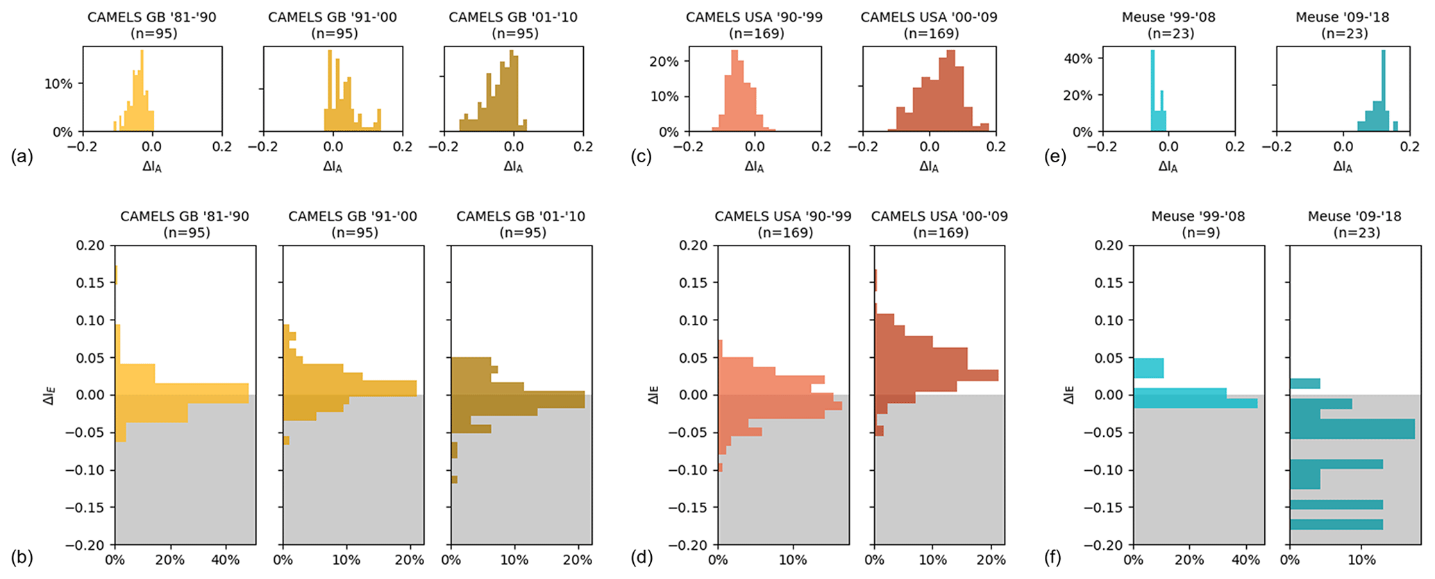
Figure 8 Distributions of ΔI_A per decade and per data set, CAMELS GB (a), CAMELS USA (c), and Meuse (e), and the deviations in estimating I_E (ΔI_E) for the different data sets of CAMELS GB (b), CAMELS USA (d), and Meuse (f).

Figure 9 (a) I_E deviations (ΔI_E) plotted per aridity index in the Budyko framework for all data sets combined, (b) distributions of I_E deviations (ΔI_E) corresponding to the aridity index groups from (a), (c) distributions of I_E deviations (ΔI_E) for all data combined and for Meuse data.

The noticeable and significant shift towards higher, i.e. more positive, ΔI_E,US between these decadal distributions entails proportionally higher-than-expected evaporation for the later decade. In contrast, while, for the first decade, the catchments in Meuse basin have a median $\mathrm{\Delta }{I}_{\mathrm{E},\mathrm{Meuse}}\sim \mathrm{0}$ that is broadly consistent with those of the GB and the US catchments, the distribution experiences a major shift towards lower, i.e. more negative, values, with a median $\mathrm{\Delta }{I}_{\mathrm{E},\mathrm{Meuse}}\sim -\mathrm{0.06}$ in the second decade, suggesting lower-than-expected proportional evaporation. However, this pattern may be an artefact of the limited sample sizes, consisting of only 9 and 23 catchments in the first and second decades, respectively, in the Meuse basin and should be interpreted with due care to avoid misinterpretations.

In the deviations ΔI_E from the expected I_E, no apparent geographical pattern can be distinguished through visual analysis (Fig. S4). In particular, for GB, adjacent catchments do frequently display opposing signs in ΔI_E, indicating positive and negative deviations from expected I_E within very close distances.

Similarly, aggregating the individual distributions of ΔI_E of all three data sets and all decades into one full distribution and stratifying this distribution into individual distributions according to their aridity index I_A in bins of 0.2 width (Fig. 9) also does not exhibit systematic differences between the distributions. The median of all five distributions with ΔI_E=0.00–0.01 close to zero and their spreads are characterised by only minor differences, with values of IQR ∼ 0.02 for I_A=0.2–0.4 and IQR ∼ 0.06 for I_A=0.8–1.0. For additional context, the individual values of ΔI_E for each catchment are plotted against the corresponding ΔI_A, illustrating that, overall, the variability from catchment to catchment is much greater than for single catchments through time (Fig. S8).

To avoid the need to base the further analysis in the Meuse exclusively on the small sample of ΔI_E,Meuse, we initially intended to construct more robust estimates of ΔI_E in the Meuse by further stratifying the above according to hydro-climatic and landscape indicators. However, this further attempt to find multi-variate relationships that link ΔI_E with hydro-climatic and landscape indicators did not show clear and consistent results and is not further reported on here. As an alternative, we therefore decided to use two extreme cases of distributions to sample ΔI_E for the Meuse basins, i.e. scenario A and scenario B (Fig. 9c; Sect. 3.2.2), in the subsequent modelling experiment. Based on the results above, the rationale behind using scenario A is that the full distribution ΔI_E describes a large sample of catchments. In the absence of a clear pattern with regard to which distribution of deviations ΔI_E is more suitable for which type of environment, the full distribution, combing all data, allows a conservative perspective as it contains a wide range of historically observed ΔI_E in a wide range of different environments. In addition, note that the full distribution of ΔI_E from all data, with a median ΔI_E=0.01 and IQR = 0.04, is very similar to the distribution associated with the I_A bin 0.6–0.8, into which most of the Meuse basins fall. The use of the full ΔI_E distribution in scenario A is contrasted by scenario B and its small sample distribution ΔI_E,Meuse. The rationale of scenario B is to conserve potentially relevant regional information that is contained in ΔI_E,Meuse and which may be under-represented in the full distribution due to the differences in the sample sizes.

4.2 Historical S_r,max and its deviations ΔS_r,max from expected values over time

The general pattern of S_r,max estimated from historical water balance data following the procedure described in Sect. 3.2 is broadly consistent with previous studies (Gao et al., 2014; Wang-Erlandsson et al., 2016; de Boer-Euser et al., 2016; Stocker et al., 2023) and reflects the overall role of hydro-climatic conditions as a control in water storage in the root zone of vegetation (Fig. 10a). While, in catchments in humid regions with low I_A, root zone storage capacities as low as $S_{\mathrm{r},\max }<\mathrm{100}$ mm are predominant, more arid regions with I_A>1 are characterised by significantly higher values of $S_{\mathrm{r},\max }>\mathrm{300}$ mm. In other words, vegetation in humid climates has developed smaller root systems due to shorter and less frequent dry spells, which ensure more regular rainwater supply that can be directly used for transpiration. In contrast, vegetation in arid climates requires more extensive root systems to access sufficient water throughout the longer and more frequent dry spells.

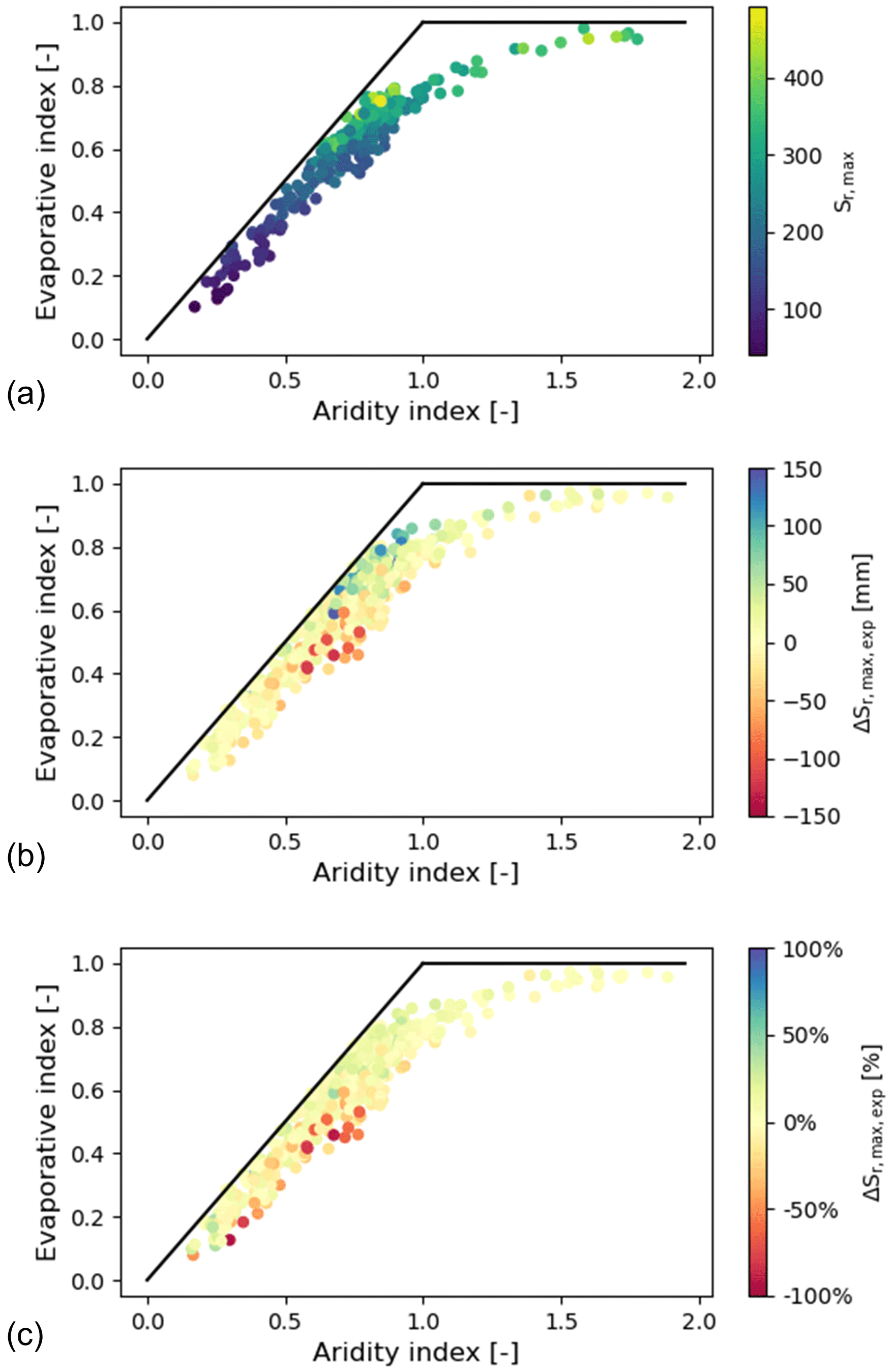
Figure 10 (a) Root zone storage capacities (S_r,max) in the Budyko framework for the Meuse, CAMELS GB, and CAMELS USA catchments. Panels (b) and (c) show the error in estimating the root zone storage capacity ($\mathrm{\Delta }{S}_{\mathrm{r},\max ,\exp }$) plotted in the Budyko framework by colour scale in absolute values (mm) and in percentages (%), respectively.

The changing hydro-climatic conditions between periods p₁ and p₂, expressed as changes in I_A in Fig. 8, resulted in shifts in $\mathrm{\Delta }{S}_{\mathrm{r},\max ,\mathrm{obs}}$ for p₂. Depending on the data set, the median $\mathrm{\Delta }{S}_{\mathrm{r},\max ,\mathrm{obs}}$ was between −24.9 for the Meuse data set and 13.6 mm for the US data set (Fig. 11). The deviations ΔI_E (Sect. 4.1) between p₁ and p₂ then caused corresponding deviations $\mathrm{\Delta }{S}_{\mathrm{r},\max ,\exp }$ from the expected $S_{\mathrm{r},\max ,\exp }$. The results illustrate that the absolute magnitudes and spreads of the deviations from expected root zone storage capacities, i.e. $\mathrm{\Delta }{S}_{\mathrm{r},\max ,\exp }$, remain, in general, rather limited and closely centred around zero (Fig. 11), with a median $\mathrm{\Delta }{S}_{\mathrm{r},\max ,\exp }=\mathrm{1.39}$ mm (IQR = 19.2 mm) in GB and slightly more pronounced values of $\mathrm{\Delta }{S}_{\mathrm{r},\max ,\exp }=\mathrm{13.6}$ mm (IQR = 43.7 mm) in the US. The relative deviations show a similar picture, with medians of 0.8 % (IQR = 11.9 %) in GB and 4.8 % (IQR = 16.5 %) in the US. Reflecting the higher ΔI_E,Meuse, $\mathrm{\Delta }{S}_{\mathrm{r},\max ,\exp }$, with a median of −24.9 mm, is characterised by more marked negative deviations in the Meuse basin, suggesting that the expected root zone storage capacity is overestimated and therefore smaller than expected.

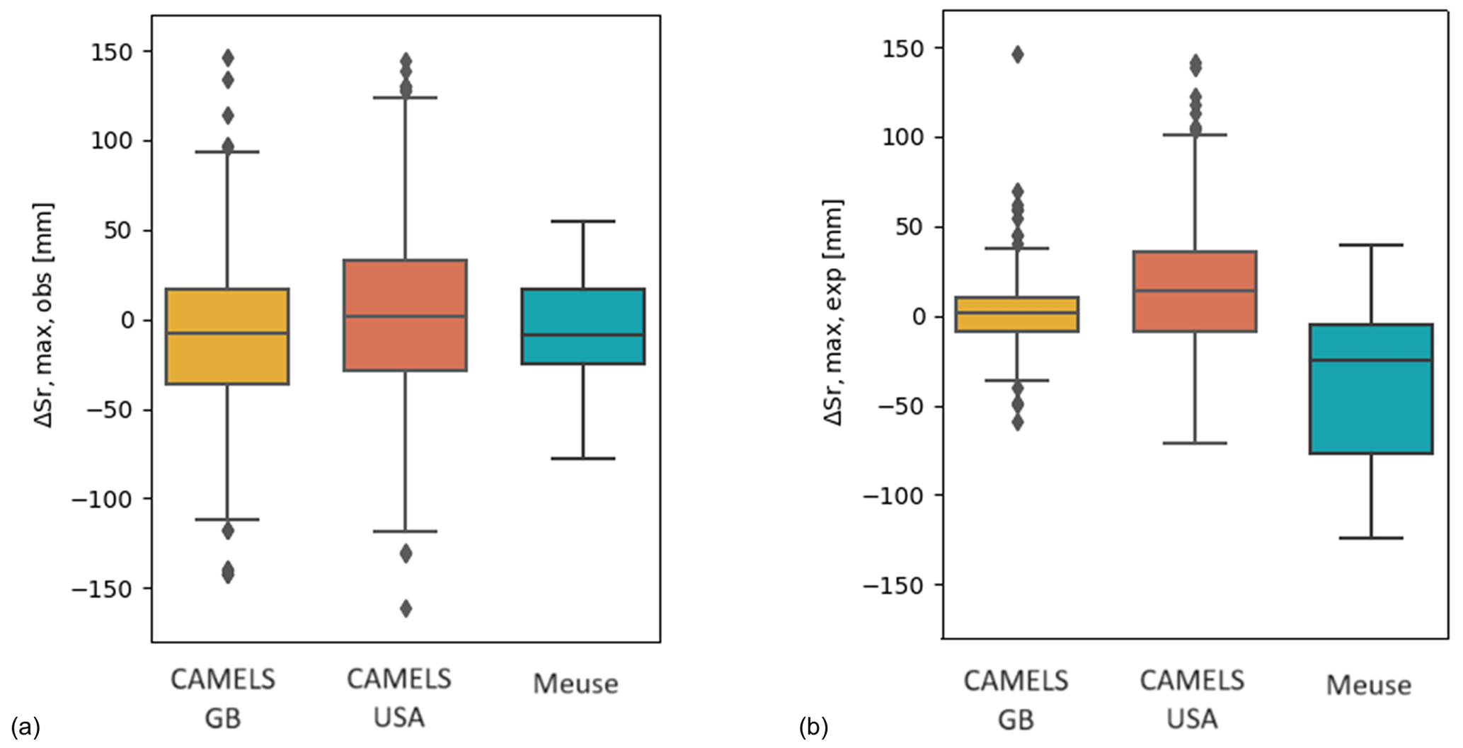
Figure 11 The distributions of shifts in (a) $\mathrm{\Delta }{S}_{\mathrm{r},\max ,\mathrm{obs}}$ observed root zone storage capacity and (b) $\mathrm{\Delta }{S}_{\mathrm{r},\max ,\exp }$ expected root zone storage capacity for the different data sets.

As shown in Fig. 10, both the absolute and relative magnitudes of $\mathrm{\Delta }{S}_{\mathrm{r},\max ,\exp }$ do not show a clear relationship with I_A. Throughout all types of environments, from humid to arid, most deviations  $\mathrm{\Delta }{S}_{\mathrm{r},\max ,\exp }$ remain closely confined to the range of −25 to 25 mm or −5 % to 5 % in relative terms. The only exception is that the highest positive and negative $\mathrm{\Delta }{S}_{\mathrm{r},\max ,\exp }$ values occur in the 0.75–1.0 aridity bin, with absolute values reaching extremes of −124 and +147 mm. However, it is noteworthy that the positive extremes in absolute changes concur with the highest magnitudes of S_r,max (Fig. 10a and b) so that the relative values of $\mathrm{\Delta }{S}_{\mathrm{r},\max ,\exp }$ in that aridity bin are largely consistent with those in more arid and more humid environments (Fig. 10c).

4.3 Effect of ΔS_r,max on streamflow predictions

4.3.1 Overall model performance

The model calibrated according to observed streamflow at the station of Borgharen at the outlet of the Meuse basin captures the main features of the hydrological response at that location. Slightly underestimating low flows and overestimating a few peaks, such as in January 2011, the model performance at Borgharen was obtained as E_NS=0.85, $E_{\mathrm{NS},\log }=\mathrm{0.72}$, and E_KG=0.88 (Fig. S9a). This is mirrored by the model's ability to reproduce streamflow in the remaining 22 sub-catchments (Fig. S9b and c), which largely exhibit only moderately lower performances, with medians of E_NS=0.72, $E_{\mathrm{NS},\log }=\mathrm{0.75}$, and E_KG=0.80 (Fig. S9d). However, for two of the catchments (Modave and Jemelle), the model could not reproduce well the hydrological response. The underlying geology of these catchments is complex, and they are likely to experience major groundwater losses which are not accounted for in this model (Bouaziz et al., 2018).

4.3.2 Changes in the hydrological response due to ΔS_r,max – scenario A

Sampling from the full distribution ΔI_E of all 286 catchments, as described in Sect. 3.3.2, and re-running the model for period p₂ with the associated values ΔS_r,max, the resulting modelled evaporation and streamflow were compared to that of the baseline scenario (ΔI_E=0 and $\mathrm{\Delta }{S}_{\mathrm{r},\max }=\mathrm{0}$). Overall, it was found that the modelled annual average evaporation and streamflow were affected only to a minor degree by ΔS_r,max with respect to the baseline scenario, with median values of between $\mathrm{\Delta }{E}_{\mathrm{A}}<\sim \mathrm{5}$ mm yr⁻¹ (<1 %) and $\mathrm{\Delta }Q>\sim -\mathrm{6}$ mm yr⁻¹ (−1 %) for all catchments.

However, minor but distinguishable shifts in the seasonal re-distribution of water fluxes compared to the baseline scenario could be observed. E_A from early summer to early autumn increases, on average, by up to ∼0.5 mm per month, depending on the catchment. In relative terms, this is equivalent to increases of up to ∼0.6 % (Fig. 12a). More specifically, at the station of Borgharen, ΔS_r,max causes the highest annual change in June, with a median ΔE_A of approximately 0.4 mm per month (∼0.5 % Fig. 12b). Similar changes can be observed in other catchments (Figs. 12c and d and S10–S32). Higher summer E_A due to ΔS_r,max is contrasted by reduced winter streamflow, which generally reaches values of ΔQ that do not exceed $\pm \sim -\mathrm{0.3}$ mm per month ($\sim -\mathrm{1}$ %; Fig. 12e). At Borgharen, the most pronounced changes occur in December, with median ΔQ of approximately -0.1 mm per month ($\sim -\mathrm{1}$ %; Fig. 12f).

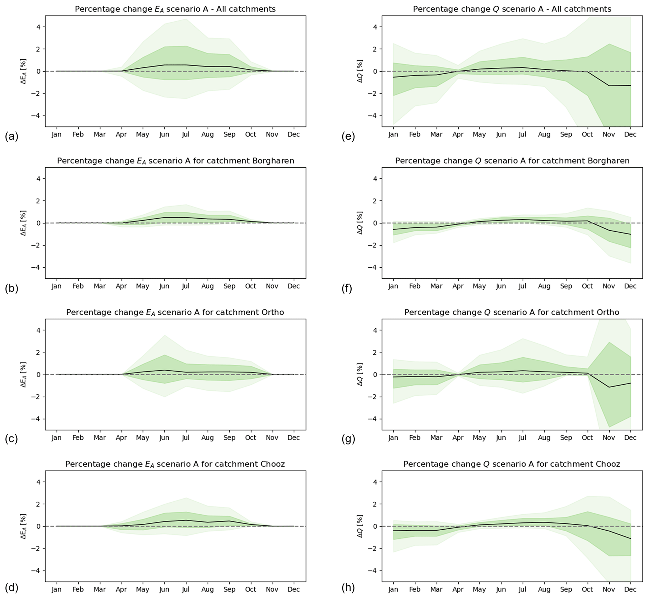
Figure 12 Change in evaporation and streamflow for scenario A. The change is calculated for every run as the difference between the evaporation (a–d) or streamflow (e–h) in relation to the reference run (ΔI_E=0). The outputs for all years and runs have been put together. The lightly shaded area represents the 90th and 10th percentiles, while the slightly darker shaded area represents the 25th to 75th percentiles. The black line represents the median. Images (a) and (e) display all catchments, (b) and (f) display Borgharen, (c) and (g) display Ortho, and (d) and (h) display Chooz.

Differences between the baseline scenario and scenario A also remain rather limited in terms of modelled annual maximum flow with a median ΔQ_max of approximately -0.1 mm d⁻¹ ($<-\mathrm{1}$ %) across all 23 study catchments in the Meuse basin (Fig. 13a). The most pronounced ΔQ_max of approximately -0.3 mm d⁻¹ ($\sim -\mathrm{1}$ %) was observed in the Le Mouzon Circourt-sur-Mouzon catchment, while, at Borgharen, $\mathrm{\Delta }{Q}_{\max }\sim -\mathrm{0.1}$ mm d⁻¹ ($\sim -\mathrm{1}$ %) was found (Fig. 13b). Annual minimum flows experienced only negligible overall increases of ΔQ_min≪1 % caused by ΔS_r,max (Fig. 13a).

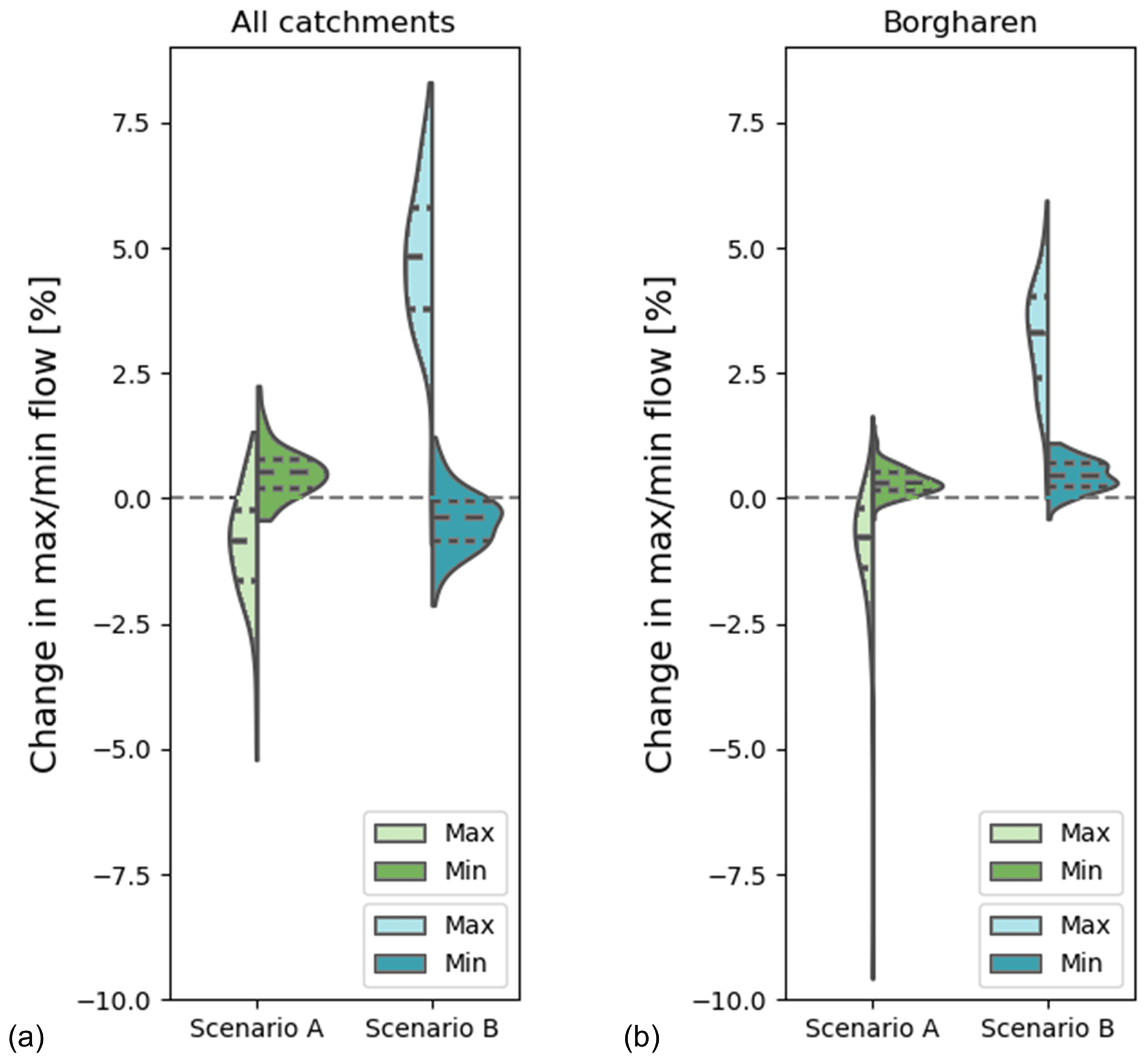
Figure 13 Change in maximum flow (Q_max, left part of the violin) and 7 d minimum flow (Q_min, right part of the violin) in terms of percentage of the reference run. The quartiles are indicated with dashed lines for (a) all catchments and (b) Borgharen.

4.3.3 Changes in the hydrological response due to ΔS_r,max – scenario B

Alternatively, sampling from the sparse, regional distribution ΔI_E,Meuse as described in Sect. 3.3.2 to estimate ΔS_r,max for model re-runs provided a perspective on how more extreme, regionally confined distributions of ΔI_E may affect the hydrological response. Similarly to scenario A, the modelled average annual changes of ΔE_A does not exceed $\sim -\mathrm{38}$ mm yr⁻¹ ($\sim -\mathrm{4}$ %) and ΔQ does not exceed ∼44 mm yr⁻¹ (∼12 %) compared to the baseline scenario. The effects of ΔS_r,max thus remained modest across all study catchments in the Meuse basin, albeit being slightly more pronounced than for scenario A.

In contrast, major differences were detected in the modelled seasonal water fluxes. On average, catchments experienced a reduction in summer evaporation, particularly in the months June and July, with ΔE_A reaching up to $\sim -\mathrm{3}$ mm per month (−4 %), as shown in Fig. 14a. Zooming in to the selected stations of Borgharen, Ortho, and Chooz, a corresponding pattern of ΔE_A can be found (Fig. 14b–d), with the most pronounced ΔE_A at -0.56 mm per month (−1 %), at station La Meuse Goncourt (Fig. S29). Seasonal streamflow experienced partly considerable increases. The modelled increases ΔQ were, on average, most pronounced in late autumn and early winter across all catchments, with median increases of up to ∼3 mm per month (∼12 %) in November and ∼4 mm per month (∼8 %) in December (Fig. 14e). Similarly, at Borgharen, median increases of $\mathrm{\Delta }Q=\sim \mathrm{1}$ mm per month (∼12 %) in November, accompanied by minor decreases in the summer months, were found (Fig. 14f).

Figure 14 Change in evaporation and streamflow for scenario B. The change is calculated for every run as the difference between the evaporation (a–d) or streamflow (e–h) in relation to the reference run (ΔI_E=0). The outputs for all years and runs have been put together. The lightly shaded area represents the 90th and 10th percentiles, while the slightly darker shaded area represents the 25th to 75th percentiles. The black line represents the median. Images (a) and (e) display all catchments, (b) and (f) display Borgharen, (c) and (g) display Ortho, and (d) and (h) display Chooz.

The modelled annual maximum flows increased through for scenario B, with a median ΔQ_max of approximately 0.35 mm d⁻¹ (∼5 %) across all study catchments in the Meuse basin (Fig. 13a). The most pronounced ΔQ_max of 1 mm d⁻¹ (∼6 %) was observed in the La Meuse Goncourt catchment, while, at Borgharen, ΔQ_max∼0.2 mm d⁻¹ (∼5 %) was found (Fig. 13b). In spite of these partly marked increases in Q_max, the effect of ΔS_r,max on annual minimum flows in scenario B remained low and comparable to that from scenario A. For all catchments, ΔQ_min was found to be close to zero (Fig. 13a and b).

5 Discussion

Parametric formulations of the Budyko hypothesis, such as the Tixeront–Fu equation (Eq. 1; Tixeront, 1964; Fu, 1981), have, in the past, been used to predict I_E and, thus, future water partitioning based on changes in I_A under the assumption that catchments follow their specific curves in the I_A–I_E space, as defined by parameter ω that is obtained from long-term historical water balance data (Roderick and Farquhar, 2011; Wang et al., 2016; Liu et al., 2020). Recently, several studies correctly observed that catchments do not necessarily follow their specific curves under changing environmental conditions, raising the concern that parametric Budyko-style equations may therefore have little predictive power (Berghuijs and Woods, 2016; Reaver et al., 2022; Jaramillo et al., 2022). The absolute decadal fluctuations $\mathrm{\Delta }{I}_{\mathrm{A}}=-\mathrm{0.05}$ to 0.11 across all data sets in our study are rather minor and closely correspond to those reported by previous studies (e.g. Jaramillo et al., 2022; Ibrahim et al., 2024), although the relative changes may be somewhat higher. Following these absolute values ΔI_A, our results indeed provide further evidence that such deviations ΔI_E from expected I_E are a widespread phenomenon. However, our results also illustrate that, although catchments do not strictly follow their specific curves at decadal timescales, the magnitude of deviations remains, overall, rather minor, with a median of ΔI_E=0.01 and an IQR = −0.01to 0.03 across all catchments in this study (Fig. 10). In spite of some differences in detail, the general distributions of ΔI_E from different data sets, regions, and hydro-climatic conditions are broadly similar, and no systematic differences linked to catchment properties or hydro-climatic conditions could be identified (Figs. 9 and 10).

The root zone storage capacity S_r,max as a core property of terrestrial hydrological systems and parameters in hydrological models can, together with its evolution over time, be robustly estimated at the catchment-scale based on water balance data (Gao et al., 2014; de Boer-Euser et al., 2016; Wang-Erlandsson et al., 2016; Dralle et al., 2021; Hrachowitz et al., 2021; McCormick et al., 2021; van Oorschot et al., 2021, 2024; Stocker et al., 2023). This offers an opportunity to account for vegetation adaptation to changing hydro-climatic conditions with a time-variable parameter S_r,max for predictions with hydrological models. Bouaziz et al. (2022) were the first to demonstrate the potential of doing that in a recent proof-of-concept study. However, they estimated future S_r,max under the assumption that their catchments will strictly follow their specific curves in the I_A–I_E space as determined by parameter ω, which was obtained from historical water balance data. In other words, they did not account for deviations ΔS_r,max that result from deviations ΔI_E. In addition, the analysis of Bouaziz et al. (2022), predicting future streamflow based on projected future water balance data, remained a scenario analysis which they could not evaluate against actual observations. Sequentially addressing these knowledge gaps, here, we quantify distributions ΔI_E from historical observed water balance data and used these observed past deviations ΔI_E to estimate past deviations ΔS_r,max, which were not accounted for by Bouaziz et al. (2022). In a first step, we found that, for the vast majority of the 286 catchments analysed in this study, characterised by a median historical S_r,max of 239.2 mm, the limited deviations ΔI_E also resulted in ΔS_r,max that remained narrowly confined between $\sim -\mathrm{10}$ to 25 mm or −5 % to 10 % (Fig. 11), although some regional outliers can reach higher values.

In a second step, using samples of ΔI_E from two distinct distributions in scenarios A and B, we estimated ΔS_r,max for use as parameter in model simulations. Overall, it was found with the more balanced scenario A that ΔS_r,max caused shifts in seasonal E_A and Q; however, this was characterised by marginal magnitudes, with the most pronounced changes in ΔE_A<1 % occurring, on average, in June and those in$\mathrm{\Delta }Q\sim -\mathrm{1}$ % occurring in December, with a similar pattern for the annual maximum and minimum flows, ΔQ_max and ΔQ_min, respectively. For scenario B, with an example of a rather extreme, regionally confined ΔI_E, the deviations showed somewhat higher magnitudes, with $\mathrm{\Delta }{E}_{\mathrm{A}}\sim -\mathrm{4}$ % in July and ΔQ∼12 % in November, and a comparable pattern for ΔQ_max and ΔQ_min.

Notwithstanding the above, it is important to bear in mind that, as in any catchment-scale hydrological experiment, the available data may be subject to various types of uncertainties, which can be further exacerbated by decisions made in the modelling process (e.g. Beven, 2016; Nearing et al., 2016; Hrachowitz and Clark, 2017; McMillan et al., 2018), so that results have to be interpreted with due care. This is particularly true for the use of long time series of data records generated by different data providers, potentially also using changing observation methods over time and for which, in many cases, homogenisation to make them comparable is not a trivial task. In this study, the use of E-OBS precipitation data, together with streamflow data, from various data providers in Belgium, France, and the Netherlands for the Meuse basin, as well as the initial analysis of the CAMELS GB and US data sets, illustrated the presence of systematic differences in the water balances between the three individual groups of data sets. These differences could, in the preliminary analysis conducted here, largely be attributed to different methods to estimate E_P. While, for the data record of the Meuse basin, the lack of more detailed consistent long-term data dictated the use of the Makkink equation based on temperature and incoming shortwave radiation, E_P was estimated using the Penman–Monteith method in the CAMELS GB catchments and using the Priestley–Taylor method in the CAMELS US catchments. In an attempt to homogenise across the data sets, we therefore re-estimated E_P in the GB and US catchments with the Makkink equation. Its simplicity and the exclusion of factors such as vapour pressure deficit or wind speed may have the potential to cause a certain level of uncertainty, although this has previously been shown to produce plausible estimates of E_P for use in hydrological models (Oudin et al., 2005).

Another unresolved issue that emerged from our analysis is the considerable reduction in evaporation in the Meuse basin between the two study periods p₁ (1999–2008) and p₂ (2009–2018), as illustrated by the distribution of ΔI_E that is characterised by remarkably more negative bias (Fig. 9) than in any other study catchment. The origin of this pattern is unclear, but similar anomalies in the hydrological response have previously been reported for the middle 20th century by others (Fenicia et al., 2009). They put forward the hypothesis that major decadal fluctuations in I_E in the Meuse basin may have been the result of active, large-scale forest management. More specifically, forest rotation and a shift from deciduous to coniferous forest, together with an increase in average forest age towards the end of the 20th century, were hypothesised to have caused the I_E fluctuations observed in the Meuse basin. While the relationship between stand age and evaporation is still under investigation (Teuling and Hoek van Dijke, 2020), there is evidence that young forests tend to evaporate more than mature forests (e.g. Vertessy et al., 2001; Brown et al., 2005). Together with Dirkse and Daamen (2004), who noted that, in the Netherlands, changes in forest management practices from clear-cutting and increased thinning resulted in a 10-year increase in the average age of trees between 1980 and 2001, specifically from 43 to 53 years; this may indeed explain at least some of the ΔI_E observed in the Meuse basin, although it remains unclear why similar pattern were not observed elsewhere.

Together, the results of this study suggest that, although most catchments do not strictly follow their specific curves in the I_A–I_E space over time, the general magnitudes of deviations ΔI_E are, in general, low enough to cause only very minor deviations ΔS_r,max in predictions of root zone storage capacities. As a consequence, even under the assumption of rather exceptional ΔI_E and thus ΔS_r,max in scenario B, the effects on the hydrological response remain limited. This further suggests that vegetation adaptation to factors other than I_A, which are manifest in the deviations ΔI_E and, eventually, in ΔS_r,max, does not lead to major changes in the predicted future hydrological response in the Meuse basin overall. However, it is plausible to assume that, in other regions that are characterised by stronger seasonal contrasts in liquid water supply (related to both seasonal rainfall distribution and snowmelt), similar deviations in ΔI_E may lead to larger ΔS_r,max and thus more pronounced effects on streamflow dynamics. Irrespective of that and in spite of not strictly following their specific curves, catchment estimates of future I_E, based on changes in future I_A, may therefore still be considered to be useful as first-order estimates to quantify the future evolution of parameter S_r,max in hydrological models for climate impact studies over decadal timescales.

6 Conclusions

In this study, we have quantified the cascading effects of uncertainties in decadal predictions of evaporative ratios I_E as a function of changes in catchment aridity I_A on predictions of root zone storage capacities S_r,max and, eventually, on predictions of streamflow. In this study in the Meuse basin, it was found that (1) when inferred from long-term data from 286 catchments in Europe and the US that are hydro-climatically similar to the Meuse basin, catchments do not strictly follow their specific curves defined by parameter ω in the I_A–I_E Budyko space over multiple decades, but these deviations are characterised by limited magnitudes with average ΔI_E of 0.01 (0.89 %); (2) the deviations ΔI_E have a minor impact on predictions of S_r,max, with the resulting deviations ΔS_r,max ranging mostly between −10 to 20 mm or −5 % to 10 %; and, finally, (3) these uncertainties ΔS_r,max have only a limited effect on the hydrological response in the Meuse basin because, in spite of causing shifts in the seasonal water supply, the magnitudes of these shifts in monthly E_A and Q largely remain very minor (<1 %) and do not, even in the exceptional scenario B, exceed 4 % (E_A) to 12 % (Q). Overall, this suggests that uncertainties in predictions of I_E based on parametric Budyko-style equations and the associated uncertainties in predictions of model parameter S_r,max do not cause major uncertainties in streamflow predictions in the Meuse basin and can thus be considered to be useful first-order estimates in the absence of more detailed information.