the Creative Commons Attribution 4.0 License.
the Creative Commons Attribution 4.0 License.
 | 13 Sep 2024
Ratio limits of water storage and outflow in a rainfall–runoff process
Yulong Zhu
Yang Zhou
Xiaorong Xu
Changqing Meng
Yuankun Wang
Flash floods typically occur suddenly within hours of heavy rainfall. Accurate forecasting of flash floods in advance using the two-dimensional (2D) shallow water equations (SWEs) remains a challenge, due to the governing SWEs being difficult-to-solve partial differential equations (PDEs). Aiming at shortening the computational time and gaining more time for issuing early warnings of flash floods, constructing a new relationship between water storage and outflow in the rainfall–runoff process is attempted by assuming the catchment as a water storage system. Through numerical simulations of the diffusion wave (DW) approximation of SWEs, the water storage and discharge are found to be limited to envelope lines, and the discharge/water-depth process lines during water rising and falling showed a grid-shaped distribution. Furthermore, if a catchment is regarded as a semi-open water storage system, then there is a nonlinear relationship between the inside average water depth and the outlet water depth, namely, the water storage ratio curve, which resembles the shape of a plume. In the case of an open channel without considering spatial variability, the water storage ratio curve is limited to three values (i.e., the upper, the steady, and the lower limits), which are found to be independent of meteorological (rainfall intensity), vegetation (Manning's coefficient), and terrain (slope gradient) conditions. Meteorological, vegetation, and terrain conditions only affect the size of the plume without changing its shape. Rainfall, especially weak rain (i.e., when rainfall intensity is less than 5.0 mm h−1), significantly affects the fluctuations of the water storage ratio, which can be divided into three modes: Mode I (inverse S-shape type) during the rainfall beginning stage, Mode II (wave type) during the rainfall duration stage, and Mode III (checkmark type) during rainfall end stage. Results indicate that the determination of the nonlinear relationship of the water storage ratio curve under different geographical scenarios will provide new ideas for simulation and early warning of flash floods.
- Article
(3868 KB) - Full-text XML
- BibTeX
- EndNote


Flood disaster is a significant global health and economic threat. Disastrous floods have caused millions of fatalities in the 20th century and billions of dollars in direct economic losses each year (Merkuryeva et al., 2015; Merz et al., 2021; Ruidas et al., 2022). According to statistics (Lee et al., 2020), from 2001 to 2018, over 2900 floods caused over 93 000 deaths and over USD 490 billion in economic damages worldwide. Based on 250 m resolution daily satellite images of 913 major flood events during the same period, the total area inundated by floods is estimated to be 2.23×10⁶ km2, and the directly affected population is estimated to be 255 to 290 million (Tellman et al., 2021). With the influence of climate change and extreme El Niño events (Ward et al., 2014; Cai et al., 2014), flood events caused by extreme precipitation are occurring frequently in many regions around the world (Kirezci et al., 2020; Najibi and Devineni, 2018; Almazroui, 2020). From 2020 to 2023, catastrophic floods caused by several extreme rainfall events were reported in Germany (Tradowsky et al., 2023), China (Hsu et al., 2021), Italy (Valente et al., 2023), Japan (Kobayashi et al., 2023), Pakistan (Nanditha et al., 2023), and other developed or developing countries and regions, even in some desert areas, e.g., in the Taklimakan Desert and the Atacama Desert, as reported by Li and Yao (2023) and by Cabré et al. (2023), respectively. Research shows that under a high emissions scenario, at latitudes above 40° N, compound flooding could become more than 2.5 times as frequent by 2100 compared to the present (Bevacqua et al., 2020). This means that in the future, the fraction of the global population at risk of floods will be increasing.
Flood simulation provides an effective means of flood forecasting to reduce the loss of property and life in flood-threatened areas around the world. In particular, weather-prediction-based distributed hydrological/hydraulic models are considered to be an effective strategy for flood simulation (Ming et al., 2020). Hence, a large number of scholars are committed to improving the simulation efficiency or simulation accuracy of distributed hydrological/hydraulic models. Accordingly, they have developed many forms of hydrological models and hydrodynamic models in the past decades. Among them, the hydrological models include Stanford Watershed Model IV (SWM) (Crawford and Linsley, 1966), the SHE/MIKESHE model (Abbott et al., 1986), the TANK model (Sugawara, 1995), Soil and Water Assessment Tool (SWAT) (Arnold and Williams, 1987), and TOPMODEL (Beven and Kirkby, 1979). The hydrodynamic models include the one-dimensional (1D) Saint-Venant equations (Köhne et al., 2011), the two-dimensional (2D) shallow water equations (SWEs) (Camassa et al., 1994), and the three-dimensional (3D) integrated equations of runoff and seepage (Mori et al., 2015). In addition, a variety of hydrological–hydrodynamic coupling models have also been proposed by Kim et al. (2012), Liu et al. (2019), Hoch et al. (2019), and other scholars. In particular, SWEs are the main governing equations for simulating floods. However, flood simulation based on SWEs is a time-consuming process due to its governing equations being a hyperbolic system of first-order nonlinear partial differential equations (PDEs) (Li and Fan, 2017). Therefore, many scholars attempted to improve the efficiency and accuracy of flood simulation through computer technology, e.g., applying GPU parallel computing (Crossley et al., 2010) or advanced numerical schemes (Sanders et al., 2010). For hydrological studies, the performance of hydrological modeling is usually challenged by model calibration and uncertainty analysis during modeling exercises (Wu et al., 2021).
Efficient and stable solutions for hydrodynamic models has long been an important issue in flood forecasting. Since the SWEs are nonlinear hyperbolic PDEs, the increase in the calculation domain and the increase in the degree of discreteness will greatly increase the difficulty of solving SWEs. In addition, when using high-resolution terrain to improve model calculation accuracy, non-physical phenomena such as false high-flow velocity in steep terrain will also occur, resulting in calculation distortion and a sharp increase in calculation time. Hence, we try to ignore the complex exchange/transfer process of mass and momentum (hydrodynamic models), and we also abandon the empirical relationships (hydrological models) between the input (precipitation), the transmission (flow rate), and the output (discharge) in the catchment area. A catchment is regarded as a semi-open water storage system, and the complex problem is simplified into three megascopic variables, i.e., inflow, water storage, and outflow. For one watershed, the complex internal flow processes could be ignored if the physical mechanism between inflow, water storage, and outflow can be found under different meteorological, geographical, and geological conditions. In other words, if we can give a physical-based relationship between the three megascopic variables, then flood forecasting will become much simpler.
An arbitrary catchment (Fig. 1b) could be assumed to be a conceptual water tank (Fig. 1a). In this water tank, according to the law of conservation of mass, the complex confluence process of surface runoff could be neglected, and it can be described only by the relationship between input, storage, and output, which can be expressed as Eq. (1),
where A is catchment area (m2), t is time (s), H is internal average water depth (m), R is rainfall intensity (m s−1), I is infiltration (m s−1), F is exfiltration (m s−1), E is evaporation (m s−1), and Q is discharge (m3 s−1).
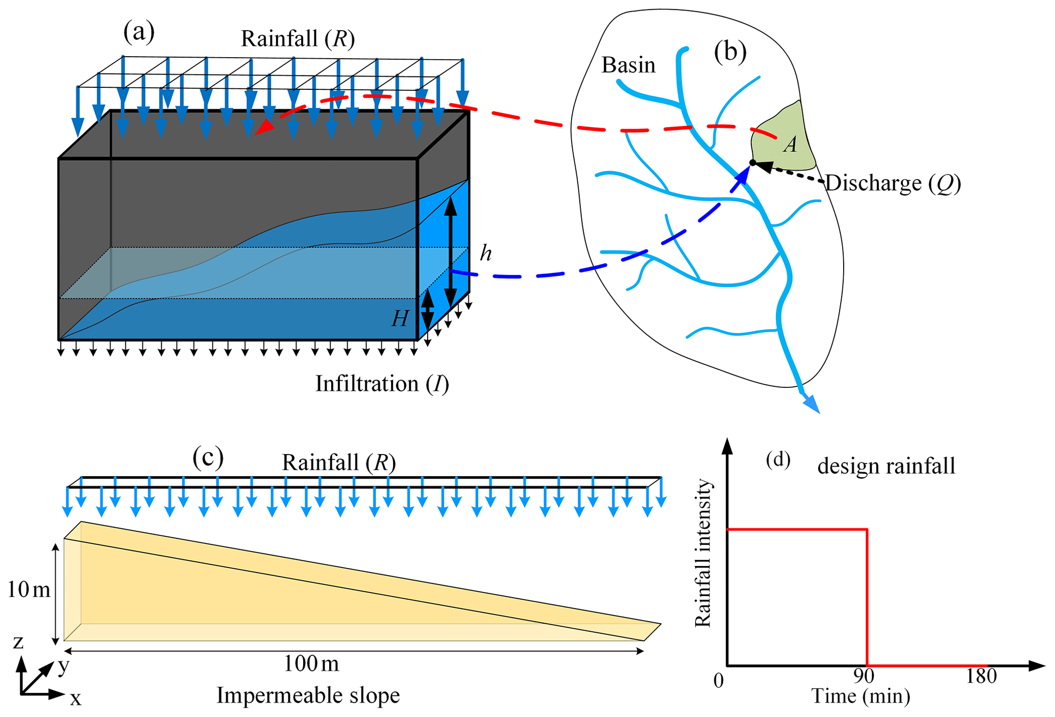
Figure 1Conceptual schematic of the distributed runoff model (DRM) and numerical model. (a) Conceptual water tank; (b) conceptual catchment; (c) impermeable conceptual slope model; (d) design rainfall.
In this section, attention is focused on the surface flow of runoff, so the runoff–atmosphere moisture exchange (evaporation) and runoff–soil moisture exchange (infiltration and/or exfiltration) are not considered. Zhu et al. (2020) validated the effectiveness of a diffusion wave (DW) approximation of shallow water equations by numerical simulations for simulating ground surface runoff,
where h is water depth (m), z is elevation (m), nm is Manning's coefficient (s m), and S is the slope gradient.
To improve the computational efficiency of the hydrodynamic model, after strict mathematical derivation according to the basic hydrodynamic equation and the law of conservation of mass, Zhu et al. (2022) proposed a hydrological–hydrodynamic integrated model, i.e., distributed runoff model (DRM), as
where is conceptual outflow (m s−1), η is the water storage ratio, and B is the outlet width (m).
The conceptual hydrological model takes the inside average water depth (H) in the catchment area as the independent variable (Eq. 1). However, the hydrodynamic equations take the water depth at any outlet (h) as an independent variable (Eq. 2). If a relationship between the inside average water depth (H) and outlet water depth (h) can be established, then this relationship will have both hydrodynamic and hydrological characteristics. Therefore, to find the H–h relationship, an impermeable conceptual slope model was built as shown in Fig. 1c, and numerical simulations were performed using the diffusion wave (DW) approximation (Eq. 2) of shallow water equations (SWEs). The water storage ratio is defined as the inside average water depth (H) divided by the outlet water depth (h). Firstly, the numerical simulations are performed under a designed rainfall condition; that is, rainfall intensity is 10 mm h−1, and rainfall duration is 90 min with a total time of 180 min as shown in Fig. 1d. From the time-dependent water storage ratio () under different catchment area (Fig. 2a), it can be seen that continuous rainfall will cause the water storage ratio () to gradually decrease from the initial value of 1.0 (upper limit) to a stable value, which is approximately 0.625 (steady limit). When the rainfall ends, the value of the water storage ratio () decreases first and then increases, showing a U-shaped curve with a lower limit, which is approximately 0.4125. Afterward, the water storage ratio curves are under 10 kinds of catchment area (Fig. 2b), three kinds of Manning's coefficient (Fig. 2c), four kinds of slope gradient (Fig. 2d), and four kinds of rainfall intensity (Fig. 2e); conditions are obtained from parametric analyses and collected in Fig. 2f.
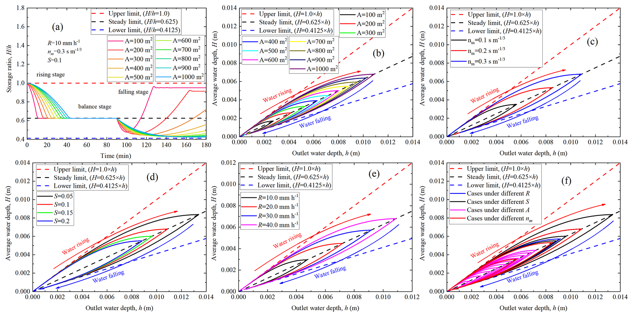
Figure 2Water storage ratio curves. (a) Time-dependent water storage ratio under different catchment areas with 10 mm h−1; (b) water storage ratio curves under 10 kinds of catchment area; (c) water storage ratio curves under three kinds of Manning's coefficient; (d) water storage ratio curves under four kinds of slope gradient; (e) water storage ratio curves under four kinds of rainfall intensity; (f) collection of the above 21 water storage ratio curves. Three limit lines envelop all water storage ratio curves, i.e., upper limit (), steady limit (), and lower limit ().
Finally, it is found that water storage ratio curves resemble the shape of a plume. When the water outlet depth is the same, the water storage ratio () of the water-rising limb is higher than that of the water-falling limb. Furthermore, in the case of an open channel without considering spatial variability, there are three limits (the upper, the steady, and the lower limits) of the water storage ratio curves, which are found to be independent of meteorological (rainfall intensity), vegetation (Manning's coefficient), and terrain (slope gradient) conditions. Meteorological, vegetation, and terrain conditions only affect the size of the plume without changing its shape which is anchored by three limits. This means that the three limits and the water storage ratio curves provide a key to establishing a relationship between the hydrodynamic models and the hydrological models.
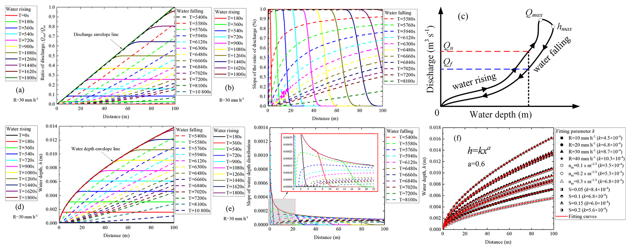
Figure 3Discharge/water-depth process lines during water rising and falling. (a) Discharge process lines during water rising and falling; (b) gradient lines of discharge process line during water rising and falling; (c) schematic diagram of looped rating curve; (d) water depth process lines during water rising and falling; (e) gradient lines of water depth process lines during water rising and falling; (f) change of water depth envelope line under different rainfall intensity (R), Manning's coefficient (nm), and slope gradient (S).
To obtain further insights into the causes of the formation of the water-rising limb and the water-falling limb of the water storage ratio curve, the ratio of discharge (i.e., the ratio of the total outflows (Qout) to the total inflows (Qin)) and the water depth (h) along the slope are discussed in Fig. 3a and d, respectively. Results indicate that there is an envelope line that controls the distribution of the discharge and water depth along the slope, respectively. The discharge envelope line is a straight line with a slope of 1 % (Fig. 3a), while the water depth envelope line is a nonlinear curve controlled by a power function of the general form h=kxa (Fig. 3d). This means that if the duration of rainfall with a constant intensity is long enough, the catchment system will eventually reach an equilibrium state between inflow and outflow.
On the other hand, the process lines of discharge and water depth during water rising and falling present a grid-shaped cross-distribution (Fig. 3a and d). Similarly, from the view of the gradient of the discharge and water depth process lines during water rising and falling, the discharge gradient curves (Fig. 3b) and the water depth gradient curves (Fig. 3e) also present a grid-shaped cross-distribution during water rising and falling, which might be the cause of the looped rating curve (Fig. 3c), i.e., higher discharges for the rising limb (Qu) than for the recession limb (Qf) at the same stage (Petersen-Øverleir, 2006). After fitting the value of parameter k and a under different rainfall intensity (R), Manning's coefficient (nm), and slope gradient (S) conditions (Fig. 3f), it is found that the parameter a is a constant, while the change of parameter k is positively correlated with the change of rainfall intensity (R) and Manning's coefficient (nm), but it is negatively correlated with the change of slope gradient (S).
Based on the water storage ratio curve, a hydrological–hydrodynamic integrated model, namely, the distributed runoff model (DRM), is established with the governing equations in Eq. (3). To check the effectiveness and applicability of the DRM, a comparative analysis of the numerical results obtained from the DRM and the DW model is implemented. We found that the DRM quickly reproduces the calculation results of the time-consuming DW model under different rainfall intensities (Fig. 4a and b), different Manning's coefficients (Fig. 4c), and different slope gradients (Fig. 4d). meaning that the water storage ratio curve will provide new ideas for simulation and early warning of floods. In addition, due to the governing equations of the DRM being ordinary differential equations (ODEs), the computational efficiency of the DRM is much higher than the DW model, which is governed by nonlinear partial differential equations (PDEs). More attention should be paid to the determination of the nonlinear relationship of the water storage ratio curve under different geographical scenarios, which will be beneficial to the proposal of more efficient flood-forecasting methods or early-warning systems.
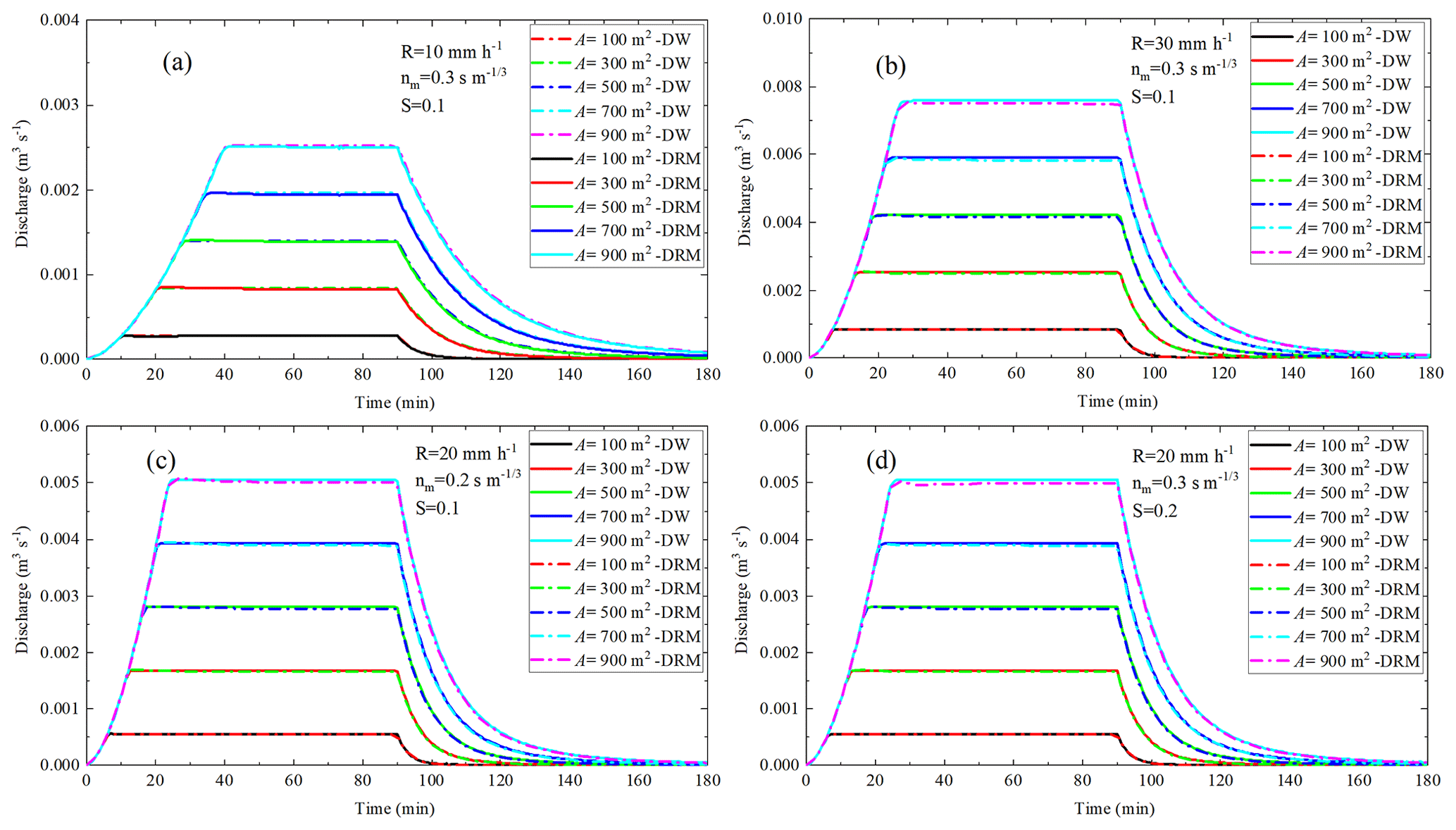
Figure 4Comparative analyses of discharge calculated by DW and the DRM under designed rainfall. (a) controlled group; (b) compared with (a), only the rainfall intensity is changed; (c) compared with (a), rainfall intensity and Manning coefficient are changed; (d) compared with (a), rainfall intensity and slope gradient are changed.
In the above section, the simulations of DW and the DRM are based on an impermeable conceptual slope model as shown in Fig. 1c. After considering infiltration in DW and the DRM, Eqs. (2) and (3) become
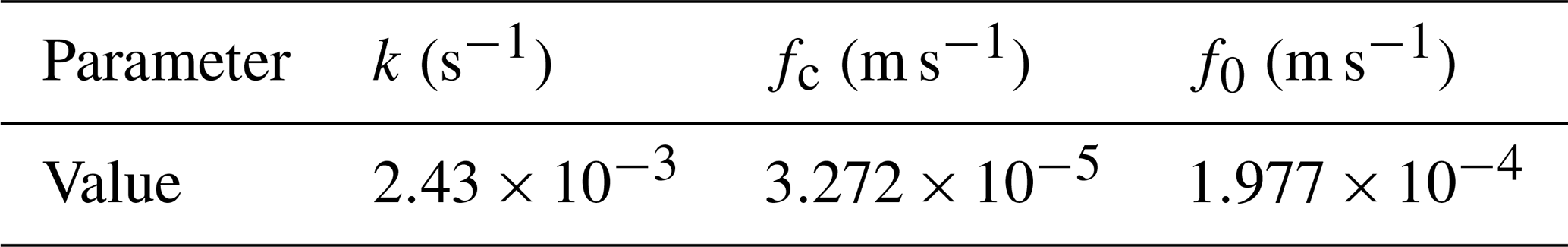
Infiltration (I) is calculated by Horton's infiltration model (Horton, 1933), which suggests an exponential equation for modeling the soil infiltration capacity fp (m s−1):
where f0 is the initial infiltration capacity (m s−1), fc is the final infiltration capacity (m s−1), and k represents the rate of decrease in the capacity (s−1). The infiltration parameter sets are listed in Table 1.
A rainfall event begins with a weak precipitation intensity. When the rainfall intensity is less than the infiltration capacity, all the rainwater will infiltrate into the soil. When the rainfall intensity exceeds the soil infiltration capacity, the surface water is generated, and Horton law (Eq. 6) applies:
Results of outlet discharge (Q) and runoff volume (ROV) calculated by DW and DRM are compared with the reference results adopted from Fernández-Pato et al. (2016) as shown in Fig. 5. Figure 5a shows the comparison of results under a uniform design rainfall. In this case, the rain volume is 75 000 m3 with a duration of 250 min. Figure 5b shows the comparison of results under a non-uniform rainfall. Rain volume is 75 000 m3 with a duration of 250 min. From Fig. 5, it can be recognized that after considering infiltration, except that the calculation results of the DRM are a little small at the end stage of rainfall, the calculation results of the DRM are still highly consistent with the calculation results of the DW model and reference results adopted from Fernández-Pato et al. (2016).
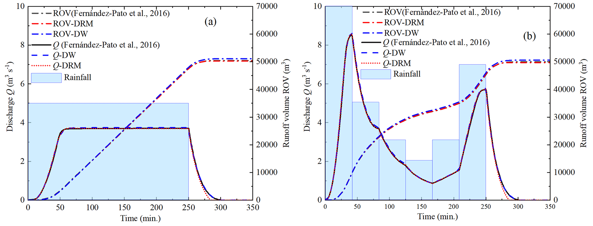
Figure 5Outlet discharge (Q) and runoff volume (ROV) calculated by DW and the DRM vs. reference results adopted from Fernández-Pato et al. (2016).
After implementing a real rainfall event in the impermeable conceptual slope model (Fig. 1c), the change in the water storage ratio is calculated as shown in Fig. 6. Rainfall data were recorded from 9 August 2022 00:00 JST (Japan standard time, UTC+9) to 10 August 2022 00:00 JST in Aomori Prefecture, Japan, and from 29 August 2016 01:00 JST to 31 August 2016 09:00 JST in Nissho Pass, Japan (https://www.data.jma.go.jp, last access: 10 August 2023). The total simulation times are 30 and 56 h, respectively. Results show that in addition to the fluctuations of water storage ratio in the beginning and end stages of rainfall, there are mainly 10 fluctuation periods of water storage ratio during the rainfall duration stage, identified as 1#, 2#, 3#, 4#, and 5# in Fig. 6a and 6#, 7#, 8#, 9#, and 10# in Fig. 6b. The fluctuations are found to be mainly caused by weak rainfall (i.e., rainfall intensity near 5.0 mm h−1) as pointed out by the red arrows in Fig. 6a and b. The magnitude of the fluctuations appears to be positively correlated with the difference between rainfall intensity and 5.0 mm h−1. When the rainfall intensity continues to be greater than 5.0 mm h−1, the fluctuation of the water storage ratio is not obvious. The water storage ratio is stable near the steady limit, even if there is heavy rainfall during this period.
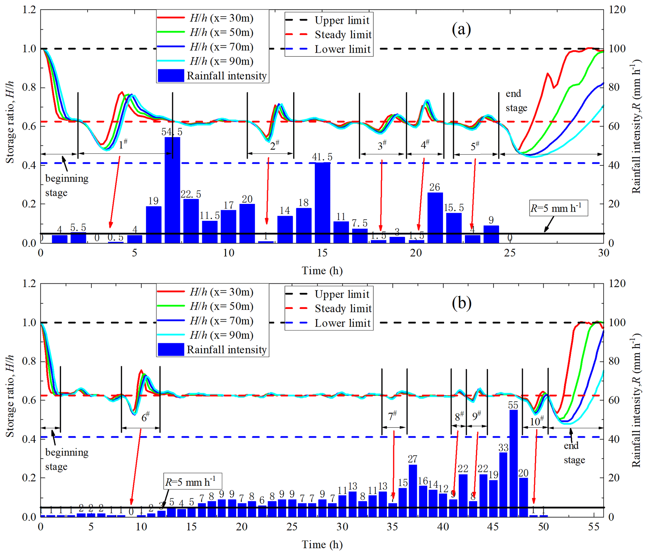
Figure 6The fluctuation of water storage ratio and the effectiveness of the DRM in natural rainfall events. (a) Aomori Prefecture; (b) Nissho Pass.
Besides, the fluctuations of the water storage ratio can be divided into three modes: Mode I identified as the inverse S-shape type during the rainfall beginning stage (Fig. 7a), Mode II identified as a wave type during the weak rainfall duration stage (Fig. 7b), and Mode III identified as a checkmark type during the rainfall end stage (Fig. 7c). Among them, Mode I describes how water storage ratio drops from the upper limit to the steady limit in an inverse S-shape. Mode II represents the water storage fluctuations around the steady limit. Mode III happens when the water storage ratio first drops from the steady limit to the lower limit and then rises to the upper limit. This means that the certainty of the fluctuation modes will provide the possibility for quantitative analysis of the fluctuation of the water storage ratio induced by the change in the rainfall intensity.
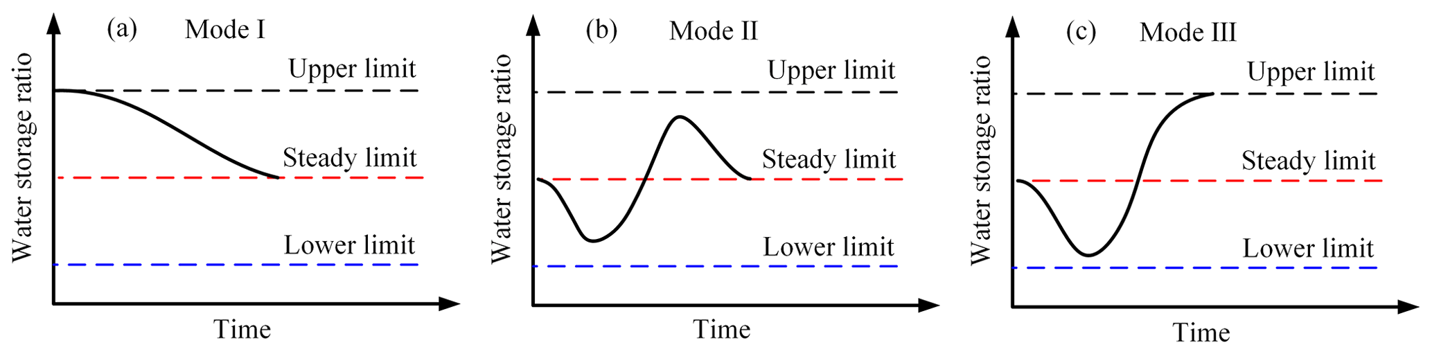
Figure 7Three kinds of water storage ratio fluctuation modes in natural rainfall events. (a) Mode I during the rainfall beginning stage; (b) Mode II during the weak rainfall duration stage; (c) Mode III during the rainfall end stage.
Figure 8a and b show the simulation results of discharge calculated by the DRM and DW model using the rainfall data recorded in Aomori Prefecture and Nissho Pass, Japan, respectively. Results suggest that after the determination of the water storage ratio fluctuations, the calculation results of the DRM are in good agreement with those of the DW model, meaning that the DRM provides a new and more effective theoretical scheme for flood prediction.
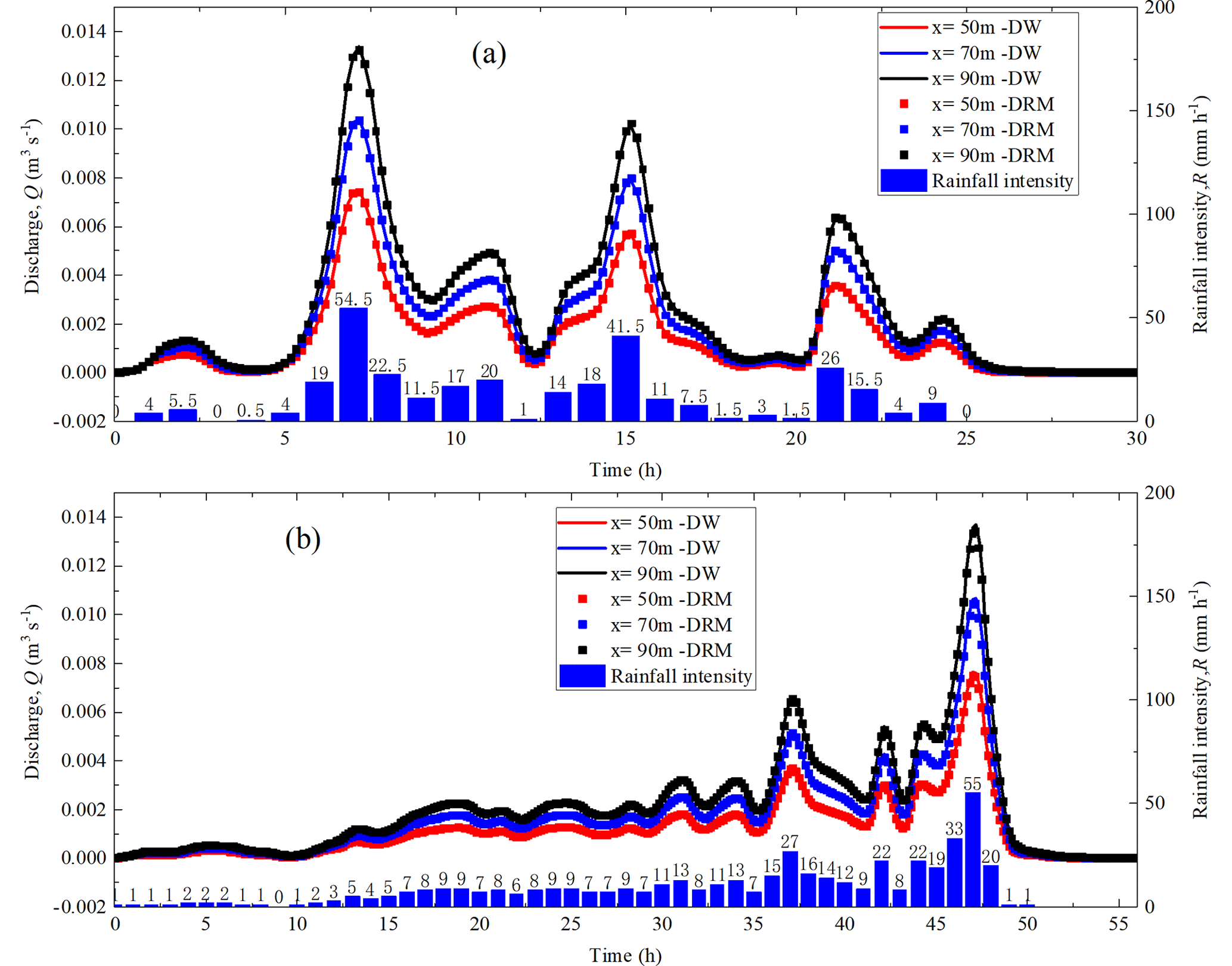
Figure 8Time-dependent discharge calculated by the DRM and DW model. (a) Aomori Prefecture; (b) Nissho Pass.
Based on a conceptual slope model, numerical simulations of the rainfall–runoff process are performed by using the diffusion wave (DW) approximation of SWEs. A plume-shaped nonlinear relationship between water storage and outflow, defined as the water storage ratio, is found between the inside average water depth and the outlet water depth in a catchment. The water storage ratio is controlled by three limits, namely, upper limit, steady limit, and lower limit with values of approximately 1.0, 0.625, and 0.4125, respectively. Under the control of the three limits, meteorological, vegetation, and terrain conditions only affect the size of the plume without changing its shape. The regular curve shape of the water storage ratio provides the possibility to construct a correlation between the water storage in the catchment area and the outlet discharge.
Based on the water storage ratio, a hydrological–hydrodynamic integrated model (DRM) is established, which shows high calculation accuracy and computational efficiency. This is because the governing equations of the DRM are ordinary differential equations (ODEs), which are much easier to solve than nonlinear partial differential equations (PDEs). However, the calculations of the DRM and DW only involve the confluence part of surface water and infiltration, while the interbasin groundwater flow as inputs to the watershed (exfiltration) and evaporation are not considered. This is inconsistent with the real rainfall–runoff process in the watershed and may lead to deviations in the calculation results. Therefore, the flow exchange between surface water and groundwater during the existence and extinction of runoff also needs to be further realized by establishing a dynamic coupling model of surface water and groundwater.
In addition, the water storage and discharge are limited to envelope lines, and the discharge/water-depth process lines during water rising and falling showed a grid-shaped distribution, which might be the cause of the looped rating curve, i.e., higher discharges for the rising limb than for the recession limb at the same stage. Rainfall, especially weak rainfall (i.e., rainfall intensity less than 5.0 mm h−1), significantly affects the fluctuations of the water storage ratio. The fluctuations of water storage ratio during a real rainfall event can be divided into three modes: Mode I identified as inverse S-shape type during the rainfall beginning stage, Mode II identified as Wave type during weak rainfall duration stage, and Mode II identified as checkmark type during rainfall end stage. It is worth noting that a qualitative determination of the three fluctuation modes of water storage ratio during rainfall events is obtained, but the quantitative analysis still needs to be further carried out in the future.
The findings in this study provide a key to establishing a simpler prediction model for flash floods. The water storage ratio has been proven to be effective in improving the effectiveness and efficiency of flood forecasting. Therefore, the determination of the nonlinear relationship of the water storage ratio curve under different geographical scenarios will provide new ideas for simulation and early warning of flash floods.
The datasets used and/or analyzed during the current study are available from the corresponding author on reasonable request.
YUZ: conceptualization, methodology, software, validation, formal analysis, investigation, data curation, writing-original draft, writing (review and editing). YAZ: methodology, validation, investigation, resources, data curation. XX: methodology, investigation, data curation. CM: validation, investigation, data curation. YW: conceptualization, methodology, writing (original draft), writing (review and editing), supervision, project administration, funding acquisition.
The contact author has declared that none of the authors has any competing interests.
Publisher’s note: Copernicus Publications remains neutral with regard to jurisdictional claims made in the text, published maps, institutional affiliations, or any other geographical representation in this paper. While Copernicus Publications makes every effort to include appropriate place names, the final responsibility lies with the authors.
This study was supported by the National Natural Science Fund of China (52279064, 52209087) and the Fundamental Research Funds for the Central Universities of China (2024MS069, 2024MS068).
This research has been supported by the National Natural Science Fund of China (grant nos. 52279064, 52209087) and the Fundamental Research Funds for the Central Universities of China (grant nos. 2024MS069, 2024MS068).
This paper was edited by Roberto Greco and reviewed by Marco Peli and one anonymous referee.
Abbott, M. B., Bathurst, J. C., Cunge, J. A., O'Connell, P. E., and Rasmussen, J.: An introduction to the European Hydrological System-Systeme Hydrologique Europeen,“SHE”, 1: History and philosophy of a physically-based, distributed modelling system, J. Hydrol., 87, 45–59, https://doi.org/10.1016/0022-1694(86)90114-9, 1986.
Almazroui, M.: Rainfall trends and extremes in Saudi Arabia in recent decades, Atmosphere, 11, 964, https://doi.org/10.3390/atmos11090964, 2020.
Arnold, J. G. and Williams, J. R.: Validation of SWRRB: Simulator for water resources in rural basins, J. Water Resour. Plan. Manage. ASCE, 113, 243–256, https://doi.org/10.1061/(ASCE)0733-9496(1987)113:2(243), 1987.
Beven, K. J. and Kirkby, M. J.: A Physically Based Variable Contributing Area Model of Basin Hydrology, Hydrol. Sci. B., 24, 43–69, https://doi.org/10.1080/02626667909491834, 1979.
Bevacqua, E., Vousdoukas, M. I., Zappa, G., Hodges, K., Shepherd, T. G., Maraun, D., Mentaschi, L., and Feyen, L.: More meteorological events that drive compound coastal flooding are projected under climate change, Communications Earth & Environment, 1, 47, https://doi.org/10.1038/s43247-020-00044-z, 2020.
Cabré, A., Remy, D., Marc, O., Burrows, K., and Carretier, S.: Flash floods triggered by the 15–17th March 2022 rainstorm event in the Atacama Desert mapped from InSAR coherence time series, Natural Hazards, 116, 1345–1353, https://doi.org/10.1007/s11069-022-05707-y, 2023.
Cai, W., Borlace, S., Lengaigne, M., van Rensch, P., Collins, M., Vecchi, G., Timmermann, A., Santoso, A., McPhaden, M. J., Wu, L., England, M. H., Wang, G., Guilyardi, E., and Jin, F. F.: Increasing frequency of extreme El Niño events due to greenhouse warming, Nat. Clim. Change, 4, 111–116, https://doi.org/10.1038/nclimate2100, 2014.
Camassa, R., Holm, D. D., and Hyman, J. M.: A new integrable shallow water equation, Adv. Appl. Mech., 31, 1–33, https://doi.org/10.1016/S0065-2156(08)70254-0, 1994.
Crawford, N. H. and Linsley, R. K.: Digital Simulation in Hydrology: Stanford Watershed Model IV, Technical Report No. 39, Department of Civil Engineering, Stanford University, 210, https://trid.trb.org/view/99040 (last access: 7 September 2024), 1966.
Crossley, A., Lamb, R., Waller, S., and Dunning, P.: Fast 2D flood modelling using GPU technology-recent applications and new developments, in: EGU General Assembly Conference Abstracts, 12043, https://api.semanticscholar.org/CorpusID:59946823 (last access: 7 September 2024), 2010.
Fernández-Pato, J., Caviedes-Voullième, D., and García-Navarro, P.: Rainfall/runoff simulation with 2D full shallow water equations: Sensitivity analysis and calibration of infiltration parameters, J. Hydrol., 536, 496–513, https://doi.org/10.1016/j.jhydrol.2016.03.021, 2016.
Hoch, J. M., Eilander, D., Ikeuchi, H., Baart, F., and Winsemius, H. C.: Evaluating the impact of model complexity on flood wave propagation and inundation extent with a hydrologic–hydrodynamic model coupling framework, Nat. Hazards Earth Syst. Sci., 19, 1723–1735, https://doi.org/10.5194/nhess-19-1723-2019, 2019.
Horton, R.: The role of infiltration in the hydrologic cycle, Trans. Am. Geophys. Union, 14, 446–460, https://doi.org/10.1029/TR014i001p00446, 1933.
Hsu, P. C., Xie, J., Lee, J. Y., Zhu, Z., Li, Y., Chen, B., and Zhang, S.: Multiscale interactions driving the devastating floods in Henan Province, China during July 2021, Weather and Climate Extremes, 39, 100541, https://doi.org/10.1016/j.wace.2022.100541, 2023.
Kim, J., Warnock, A., Ivanov, V. Y., and Katopodes, N. D.: Coupled modeling of hydrologic and hydrodynamic processes including overland and channel flow, Adv. Water Resour., 37, 104–126, https://doi.org/10.1016/j.advwatres.2011.11.009, 2012.
Kirezci, E., Young, I. R., Ranasinghe, R., Muis, S., Nicholls, R. J., Lincke, D., and Hinkel, J.: Projections of global-scale extreme sea levels and resulting episodic coastal flooding over the 21st Century, Sci. Rep.-UK, 10, 11629, https://doi.org/10.1038/s41598-020-67736-6, 2020.
Kobayashi, K., Duc, L., Kawabata, T., Tamura, A., Oizumi, T., Saito, K., Nohara, D., and Sumi, T.: Ensemble rainfall–runoff and inundation simulations using 100 and 1000 member rainfalls by 4D LETKF on the Kumagawa River flooding 2020, Progress in Earth and Planetary Science, 10, 1–22, https://doi.org/10.1186/s40645-023-00537-3, 2023.
Köhne, J. M., Wöhling, T., Pot, V., Benoit, P., Leguédois, S., Le Bissonnais, Y., and Šimůnek, J.: Coupled simulation of surface runoff and soil water flow using multi-objective parameter estimation. J. Hydrol., 403, 141–156, https://doi.org/10.1016/j.jhydrol.2011.04.001, 2011.
Lee, J., Perera, D., Glickman, T., and Taing, L. Water-related disasters and their health impacts: A global review, Progress in Disaster Science, 8, 100123, https://doi.org/10.1016/j.pdisas.2020.100123, 2020.
Li, M. and Yao, J.: Precipitation extremes observed over and around the Taklimakan Desert, China, PeerJ, 11, e15256, https://doi.org/10.7717/peerj.15256, 2023.
Li, P. W. and Fan, C. M.: Generalized finite difference method for two-dimensional shallow water equations, Eng. Anal. Bound. Elem., 80, 58–71, https://doi.org/10.1016/j.enganabound.2017.03.012, 2017.
Liu, Z., Zhang, H., and Liang, Q.: A coupled hydrological and hydrodynamic model for flood simulation, Hydrol. Res., 50, 589–606, https://doi.org/10.2166/nh.2018.090, 2019.
Merkuryeva, G., Merkuryev, Y., Sokolov, B. V., Potryasaev, S., Zelentsov, V. A., and Lektauers, A.: Advanced river flood monitoring, modelling and forecasting, J. Comput. Sci., 10, 77–85, https://doi.org/10.1016/j.jocs.2014.10.004, 2015.
Merz, B., Blöschl, G., Vorogushyn, S., Dottori, F., Aerts, J. C., Bates, P., Bertola, M., Kemter, M., Kreibich, H., Lall, U., and Macdonald, E.: Causes, impacts and patterns of disastrous river floods, Nature Reviews Earth & Environment, 2, 592–609, https://doi.org/10.1038/s43017-021-00195-3, 2021.
Ming, X., Liang, Q., Xia, X., Li, D., and Fowler, H. J.: Real-time flood forecasting based on a high-performance 2-D hydrodynamic model and numerical weather predictions, Water Resour. Res., 56, e2019WR025583, https://doi.org/10.1029/2019WR025583, 2020.
Mori, K., Tada, K., Tawara, Y., Ohno, K., Asami, M., Kosaka, K., and Tosaka, H.: Integrated watershed modeling for simulation of spatiotemporal redistribution of post-fallout radionuclides: application in radiocesium fate and transport processes derived from the Fukushima accidents, Environ. Modell. Softw., 72, 126–146, https://doi.org/10.1016/j.envsoft.2015.06.012, 2015.
Najibi, N. and Devineni, N.: Recent trends in the frequency and duration of global floods, Earth Syst. Dynam., 9, 757–783, https://doi.org/10.5194/esd-9-757-2018, 2018.
Nanditha, J. S., Kushwaha, A. P., Singh, R., Malik, I., Solanki, H., Chuphal, D. S., Dangar, S., Mahto, S. S., Vegad, U., and Mishra, V.: The Pakistan flood of August 2022: Causes and implications, Earth's Future, 11, e2022EF003230, https://doi.org/10.1029/2022EF003230, 2023.
Petersen-Øverleir, A.: Modelling looped rating curves, in: Proc., XXIV Nordic Hydrological Conference, 139–146, https://doi.org/10.13140/2.1.1069.4403, 2006.
Ruidas, D., Saha, A., Islam, A. R. M. T., Costache, R., and Pal, S. C.: Development of geo-environmental factors controlled flash flood hazard map for emergency relief operation in complex hydro-geomorphic environment of tropical river, India, Environ. Sci. Pollut. R., 30, 106951–106966, https://doi.org/10.1007/s11356-022-23441-7, 2022.
Sanders, B. F., Schubert, J. E., and Detwiler, R. L.: ParBreZo: A parallel, unstructured grid, Godunov-type, shallow-water code for high-resolution flood inundation modeling at the regional scale, Adv. Water Resour., 33, 1456–1467, https://doi.org/10.1016/j.advwatres.2010.07.007, 2010.
Sugawara, M.: The development of hydrological model-tank. Time and the River: essays by eminent hydrologists, 201–258, https://api.semanticscholar.org/CorpusID:127000384 (last access: 7 September 2024), 1995.
Tellman, B., Sullivan, J.A., Kuhn, C., Kettner, A. J., Doyle, C. S., Brakenridge, G. R., Erickson, T. A., and Slayback, D. A.: Satellite imaging reveals increased proportion of population exposed to floods, Nature, 596, 80–86, https://doi.org/10.1038/s41586-021-03695-w, 2021.
Tradowsky, J. S., Philip, S. Y., Kreienkamp, F., Kew, S. F., Lorenz, P., Arrighi, J., Bettmann, T., Caluwaerts, S., Chan, S. C., Cruz, L. D., Vries, H. d., Demuth, N., Ferrone, A., Fischer, E. M., Fowler, H. J., Goergen, K., Heinrich, D., Henrichs, Y., Kaspar, F., Lenderink, G., Nilson, E., Otto, F. E. L., Ragone, F., Seneviratne, S. I., Singh, R. K., Skålevåg, A., Termonia, P., Thalheimer, L., Aalst, M. V., Bergh, J. V. d., Vyver, H. V. d.,Vannitsem, S., Oldenborgh, G. J. V., Schaeybroeck, B. V., Vautard, R., Vonk D., and Wanders, N.: Attribution of the heavy rainfall events leading to severe flooding in Western Europe during July 2021, Climatic Change, 176, 90, https://doi.org/10.1007/s10584-023-03502-7, 2023.
Valente, M., Zanellati, M., Facci, G., Zanna, N., Petrone, E., Moretti, E., Barone-Adesi, F., and Ragazzoni, L.: Health system response to the 2023 floods in Emilia-Romagna, Italy: a field report, Prehospital and Disaster Medicine, 38, 813–817, https://doi.org/10.1017/S1049023X23006404, 2023.
Ward, P. J., Jongman, B., Kummu, M., Dettinger, M. D., Sperna Weiland, F. C., and Winsemius, H. C.: Strong influence of El Niño Southern Oscillation on flood risk around the world, P. Natl. Acad. Sci. USA, 111, 15659–15664, https://doi.org/10.1073/pnas.1409822111, 2014.
Wu, H., Chen, B., Ye, X. Guo, H., Meng, X., and Zhang, B.: An improved calibration and uncertainty analysis approach using a multicriteria sequential algorithm for hydrological modeling, Sci. Rep.-UK, 11, 16954, https://doi.org/10.1038/s41598-021-96250-6, 2021.
Zhu, Y. L., Ishikawa, T., Subramanian, S. S., and Luo, B.: Simultaneous analysis of slope instabilities on a small catchment-scale using coupled surface and subsurface flows, Eng. Geol., 275, 105750, https://doi.org/10.1016/j.enggeo.2020.105750, 2020.
Zhu, Y. L., Zhang, Y. F., Yang, J., Nguyen, B. T., and Wang, Y.: A novel method for calculating distributed water depth and flow velocity of stormwater runoff during the heavy rainfall events, J. Hydrol., 612, 128064, https://doi.org/10.1016/j.jhydrol.2022.128064, 2022.
- Abstract
- Introduction
- Methods
- Limits and plume shape of water storage ratio curve
- Grid-shaped cross-distribution of the discharge/water-depth process lines during water rising and falling
- Validation of the DRM by considering infiltration calculated by the Horton infiltration method
- Fluctuation of water storage ratio under natural rainfall conditions
- Discussions and conclusions
- Data availability
- Author contributions
- Competing interests
- Disclaimer
- Acknowledgements
- Financial support
- Review statement
- References