Technical note: Monitoring discharge of mountain streams by retrieving image features with deep learning

Traditional discharge monitoring usually relies on measuring flow velocity and cross-section area with various velocimeters or remote-sensing approaches. However, the topography of mountain streams in remote sites largely hinders the applicability of velocity–area methods. Here, we present a method to continuously monitor mountain stream discharge using a low-cost commercial camera and deep learning algorithm. A procedure of automated image categorization and discharge classification was developed to extract information on flow patterns and volumes from high-frequency red–green–blue (RGB) images with deep convolutional neural networks (CNNs). The method was tested at a small, steep, natural stream reach in southern China. Reference discharge data were acquired from a V-shaped weir and ultrasonic flowmeter installed a few meters downstream of the camera system. Results show that the discharge-relevant stream features implicitly embedded in RGB information can be effectively recognized and retrieved by CNN to achieve satisfactory performance in discharge measurement. Coupling between CNNs and traditional machine learning models (e.g., support vector machine and random forest) can potentially synthesize individual models' diverse merits and improve generalization performance. Besides, proper image pre-processing and categorization are critical for enhancing the robustness and applicability of the method under environmental disturbances (e.g., weather and vegetation on river banks). Our study highlights the usefulness of deep learning in analyzing complex flow images and tracking flow changes over time, which provides a reliable and flexible alternative apparatus for continuous discharge monitoring of rocky mountain streams.

1 Introduction

Continuous discharge data are critical for hydrological model development and flood forecast (Clarke, 1999; McMillan et al., 2010), water resources management (Council, 2004), and aquatic ecosystem health assessment (Carlisle et al., 2017). Traditional discharge monitoring relies on stream gauges that convert the water level to discharge with an established stage-discharge curve or information on stable cross sections and flow velocity obtained from flow velocimeters such as an acoustic Doppler current profiler (ADCP) and ultrasonic defectoscope (Kasuga et al., 2003). However, these approaches require significant investment into the implementation of equipment, training of personnel with expertise, and constant maintenance (Fujita et al., 2007; Czuba et al., 2017; Yorke and Oberg, 2002). Besides, the performance of transducers and velocimeters is usually susceptible to sediments and floating debris, particularly in flooding seasons (Hannah et al., 2011). Consequently, large temporal gaps remain in many discharge records across the world despite the growing demand for data (Davids et al., 2019; Royem et al., 2012). Spatially, flow monitoring of downstream river sections has been assigned a higher priority due to the concerns about water supply and flood control, leading to an acute shortage of discharge data in mountain streams and headwater catchments (Deweber et al., 2014).

To overcome the limitations of traditional methods, a few image-based approaches have been introduced into water stage, flow velocity, and discharge measurement in rivers (Noto et al., 2022; Leduc et al., 2018). Image-based approaches (Leduc et al., 2018; Noto et al., 2022) rely only on the acquisition of digital images of streams from inexpensive commercial cameras and have thus been a promising alternative for continuous, noninvasive, and low-cost streamflow monitoring. The two most commonly used approaches include large-scale particle image velocimetry (LSPIV) and particle tracking velocimetry (PTV). LSPIV (Fujita et al., 2010) is based on a high-speed cross-correlation scheme between an interrogation area (IA) in a first image and IAs within a search region (SR) in a second image. The technique has been proven to be effective in monitoring low-velocity and shallow-depth flow fields (Tauro et al., 2018). However, it performs poorly in mapping velocity fields in high resolution when there is a lack of seeds on the water surface because the algorithm obtains the average speed of each SR (Tauro et al., 2017). Compared to LSPIV, PTV was designed for low-seeding-density flows, focusing on particle tracking instead of recognition. The PTV approach does not require assumptions of flow steadiness nor the relative position of neighboring particles (Tauro et al., 2018). Several algorithms have been developed for PTV analysis, such as space–time image velocimetry (STIV) and optical tracking velocimetry (OTV), overcoming the over-dependence on natural particles' shape and size (Tauro et al., 2018; Tsubaki, 2017). STIV evaluates surface flow velocity by analyzing a texture angle within a variation in brightness or color on the water surface, while OTV combines the automatic feature detection, Lucas–Kanade tracking algorithm, and track-based filtering methods to estimate subpixel displacements (Fujita et al., 2007; Karvonen, 2016). Existing image-based discharge measurement methods all use the velocity–area method to indirectly deduce discharge after identifying stage and average velocity (Davids et al., 2019; Leduc et al., 2018; Tsubaki, 2017; Herzog et al., 2022). The average velocity in a cross section is estimated with surface velocity derived from natural or artificial seeds on water surface and pre-defined empirical relationships between the surface velocity and average velocity. The velocity–area method relies on a stable relationship between the stage and cross-sectional area and needs to take velocity extrapolations to the edges and vertical distributions throughout the cross section into account (Le Coz et al., 2012). However, it is difficult to identify the water stage and vertical characteristics of mountain streams due to the steep, narrow, and highly heterogeneous cross sections. The applicability of PIV and PTV approaches is largely hindered by such topography.

Unlike PIV and PTV, deep learning models possess the capability to extract discharge-related features from images of rivers or streams automatically. These models are able to adjust the weights assigned to each feature, eliminating the need for manual attention and reducing the risk of overemphasizing or misinterpreting features that are unresponsive to flow discharge (Canziani et al., 2016). Besides, deep learning models can extract low-level image features, such as edges, textures, and colors (Jiang et al., 2021). These merits could be essential in retrieving information from images of mountain streams, particularly in regions with intricate cross-sectional profiles. For example, Ansari et al. (2023) developed a convolutional neural network (CNN) to estimate the spatial surface velocity distribution and derive discharge, outperforming traditional optical flow methods in both laboratory and field settings, albeit with a reliance on surveyed cross-section information.

In this study, we propose a novel method for monitoring mountain stream discharge using a low-cost commercial camera and deep learning models. Automated image categorization and pre-processing procedures were developed for processing high-frequency red–green–blue (RGB) images, and then CNN was used to extract information on flow patterns from RGB matrices and establish empirical relationships with the classification probabilities of discharge volumes. We hypothesize that (1) the features of mountain streams (e.g., coverage of water surface, flow direction, flow velocity) embedded in RGB images can be recognized by suitable deep learning approaches to achieve effective discharge monitoring and (2) the proper image pre-processing and categorization can improve accuracy of image-based discharge monitoring of mountain streams. A rocky mountain stream of a headwater catchment in tropical southern China was used as a study site to test our hypotheses.

2 Methods

2.1 Site and field setting

The study site is located on a small, steep, rocky reach of a stream at the Zhuhai Campus of Sun Yat-sen University, China (22°20^′58^′′ N, 113°34^′29^′′ E). The site elevation is 13 m above sea level and about 2 km away from Lingdingyang in the South China Sea. The streamflow is mainly controlled by rainfall in the upstream drainage area. Water stage and flow velocity increase rapidly during east Asian summer monsoon rainfalls and fluctuate with synoptic weather conditions on dry days.

The main objective of the study was to test the applicability of deep-learning-based image processing approaches to capturing the flow characteristics and discharge volumes in the daily flow cycle in this mountain stream. We selected a straight, single-thread reach for the gauging location and set up a Hikvision camera on the left bank of the stream to collect flow images (Fig. 1). Discharge data monitored by a weir about 8 m downstream of the camera were used for model training and validation. The camera was installed 3 m above the ground, facing the surface of the stream almost vertically. The entire stream width is visible in the images. The camera was equipped with a 150 W solar panel and 80AH lithium battery, enabling the camera to work continuously for 80 h without external power on rainy days. The camera supports wireless transmission of video data to the server.

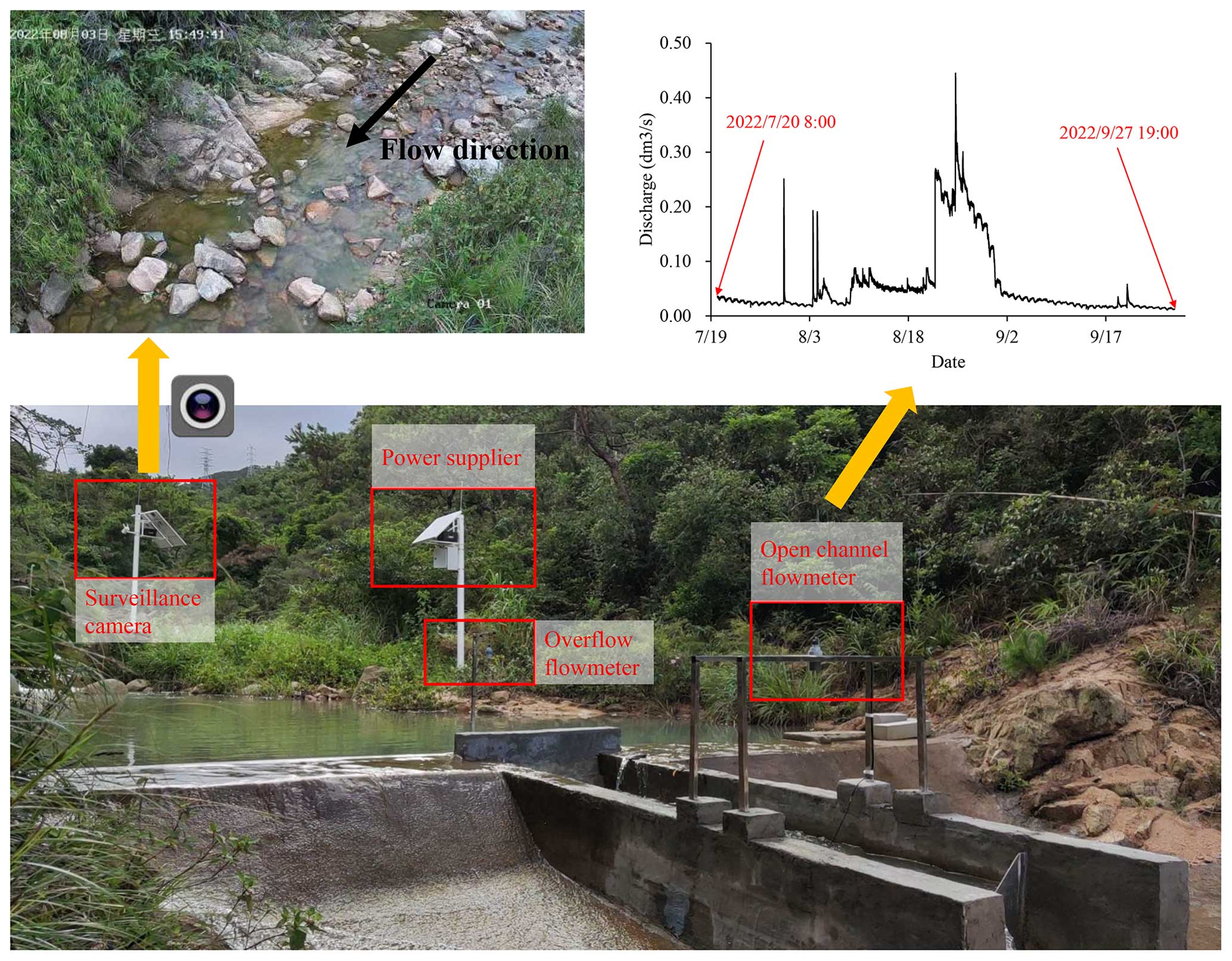
Figure 1 Camera setup. The camera is set on the left bank of the stream, about 3 m above the water surface and 8 m upstream of a gauging weir. The top-right panel demonstrates the changes in the flowmeter's discharge during the measurement period.

2.2 Data

The flat V-shaped weir downstream of the camera monitors discharge with an open-channel flowmeter and an overflow flowmeter. The flowmeters measure water levels in the channel and in front of the weir with ultrasonic sensors and calculate real-time discharge at the time step of 2 min by a semi-empirical equation suggested by the State Bureau of Technical Supervision of China (https://www.chinesestandard.net/, last access: 7 September 2024):

$$\begin{array}{}\text{(1)}& Q={\displaystyle \frac{\mathrm{8}}{\mathrm{15}}}{C}_{\mathrm{e}}\tan {\displaystyle \frac{\mathit{\theta }}{\mathrm{2}}}\sqrt{\mathrm{2}g}{h}_e^{\frac{\mathrm{5}}{\mathrm{2}}},\end{array}$$

where Q is the discharge of the stream, θ is the angle of triangular weir, g is acceleration of gravity, h_e is the height of the water surface from the bottom of the triangle barrier, and C_e is an empirical coefficient.

We collected the discharge data of the weir (Fig. 1) and its corresponding stream videos during daylight (07:00–19:00 UTC+8) from 20 July to 27 September 2022. The raw video resolution was 2560×1440 pixels, with a refresh rate of 50 Hz. Images were extracted from the videos at 5 min intervals to avoid excessive similarity between adjacent images. A total of 7757 image samples labeled with 37 discharge values between 0.014 and 0.050 m³ s⁻¹ at an interval of 0.001 m³ s⁻¹ were collected for model testing.

2.3 Image processing

2.3.1 Image categorization

Environmental disturbances such as illumination and shadow can seriously interfere with the extraction of effective image features of mountain streams, such as boundaries of water surface and textures of flow lines (Herzog et al., 2022; Gershon et al., 1986). Although researchers have proposed methods to eliminate shadows (Finlayson et al., 2002), the treatment effect in some complex environments, such as plant shadows and boulders distributed on mountain streams, is not always satisfactory.

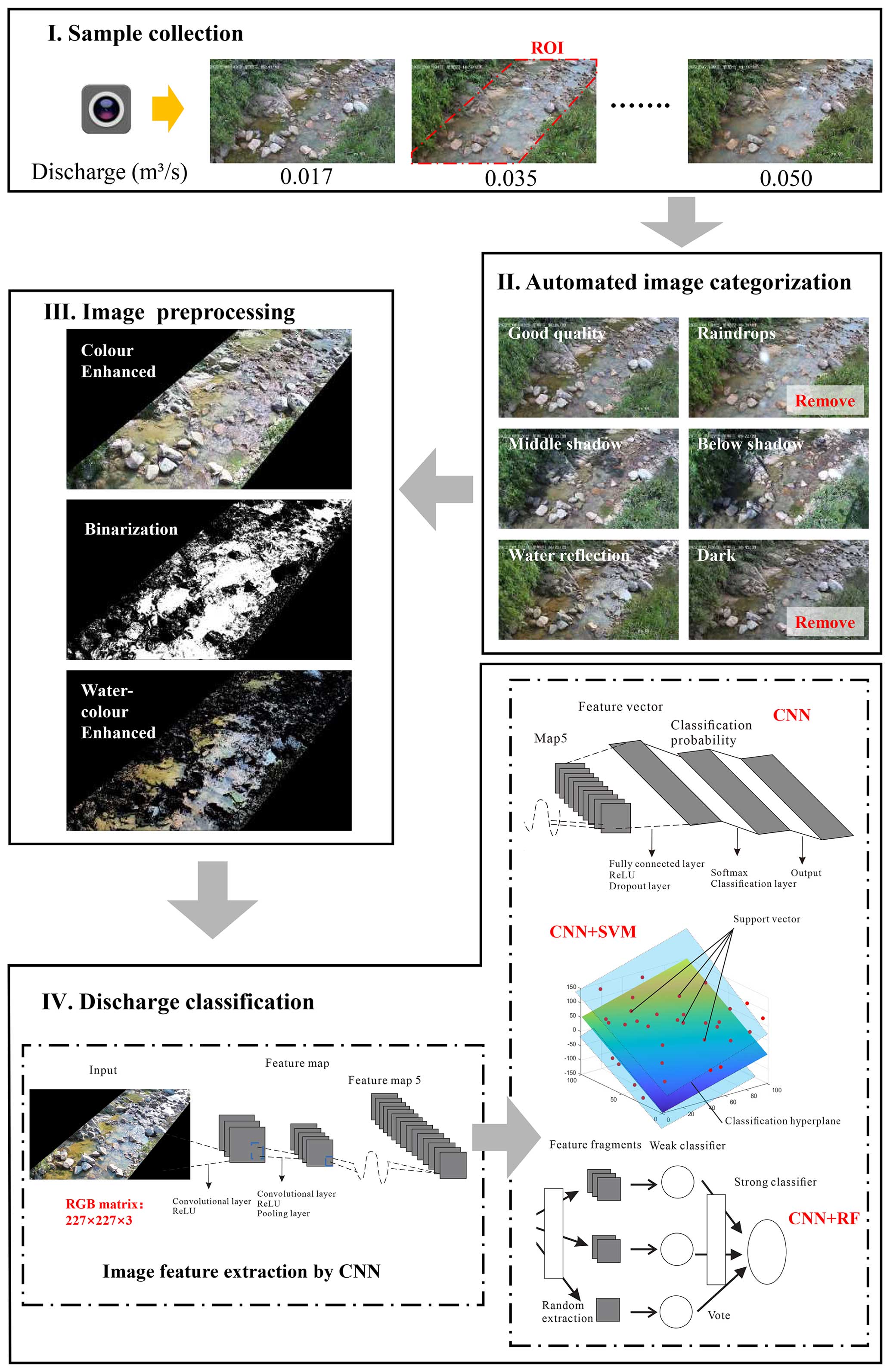
Frequently observed disturbances in images include (1) shadows in the target stream region due to plants blocking direct sunlight; (2) image noise due to raindrops attached to the camera lens on rainy days; (3) the lack of light, leading to low brightness and contrast of the image; and (4) overexposure of the image due to light reflection on the water surface (around 16:00 UTC+8 in this case). Taking these factors into consideration, we divided all image samples into six categories, including good quality, raindrops, middle shadow, below shadow, water reflection, and dark (Fig. 2). The good quality category contains image samples without obvious noise or shadow. All the other images lose some feature information due to noise, shadows, reflections, or dim lighting. To ensure the model performance under different environmental conditions, we designed an automated categorization procedure (Fig. 3) to screen the raw images and exclude the raindrops and dark samples from model training.

Figure 2 Flowchart of image processing and discharge monitoring.

Figure 3 Procedure of automated image categorization.

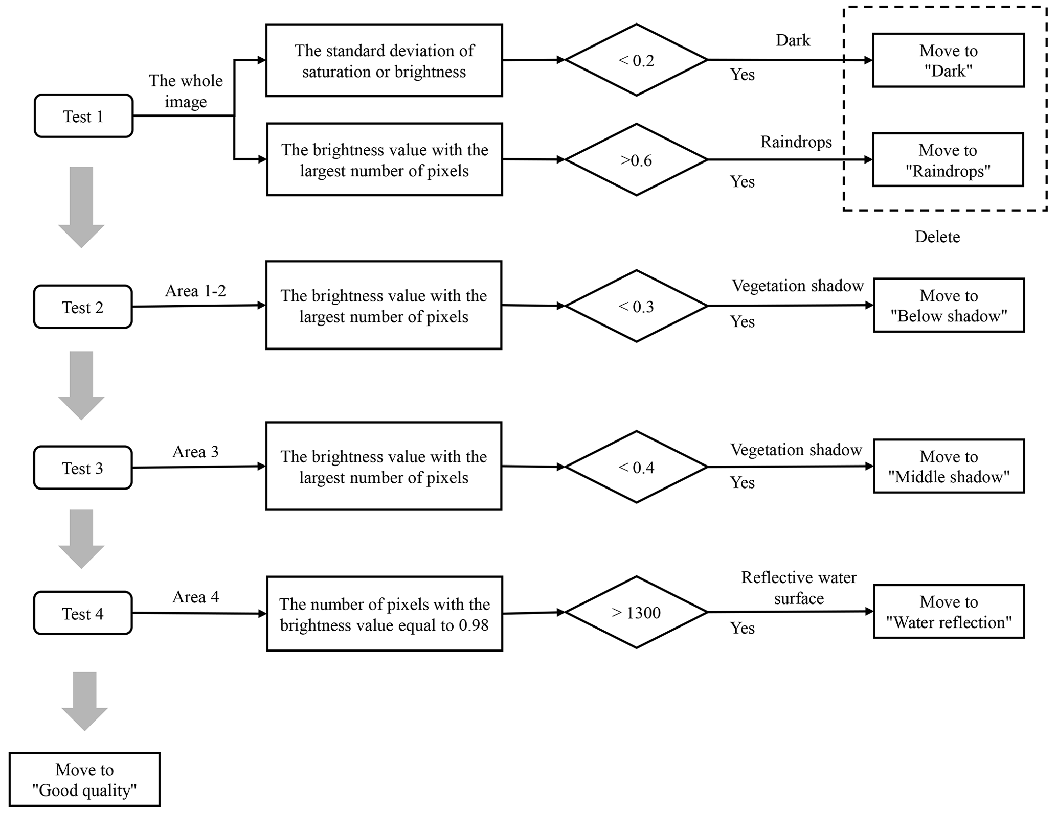
Firstly, we selected four areas in the image where the special conditions mentioned above commonly occurred to be the detection areas (Fig. 4a): the upper and lower shadows in the target stream section mainly appeared in Area 3 and Areas 1 and 2, respectively; disturbance of water surface reflection was mostly found in Area 4. Then, the thresholds of saturation or brightness in the four detection areas for image categorization were manually determined by comparing image samples under different conditions. The four-step procedure includes (1) dark images (Fig. 4f-2) were identified when the standard deviation of the brightness or saturation of the full image was lower than 0.2. (2) Raindrops images (Fig. 4f-3) were identified when the brightness of the whole image with the largest number of pixels was greater than 0.6. These two types of images were excluded from the training samples. (3) Below shadow (Fig. 4b-2 and 4c-2) and middle shadow images (Fig. 4d-2) were identified when the brightness value with the largest number of pixels in Areas 1 and 2 and Area 3 was lower than 0.3 and 0.4, respectively. (4) Water reflection images were identified when the number of pixels with a brightness value of 0.98 in Area 4 exceeded 1300 (Fig. 4e-2). The images that passed all the tests in the procedure were considered good quality samples. The other charts in Fig. 4 show the saturation and brightness distributions derived from a typical good quality image.

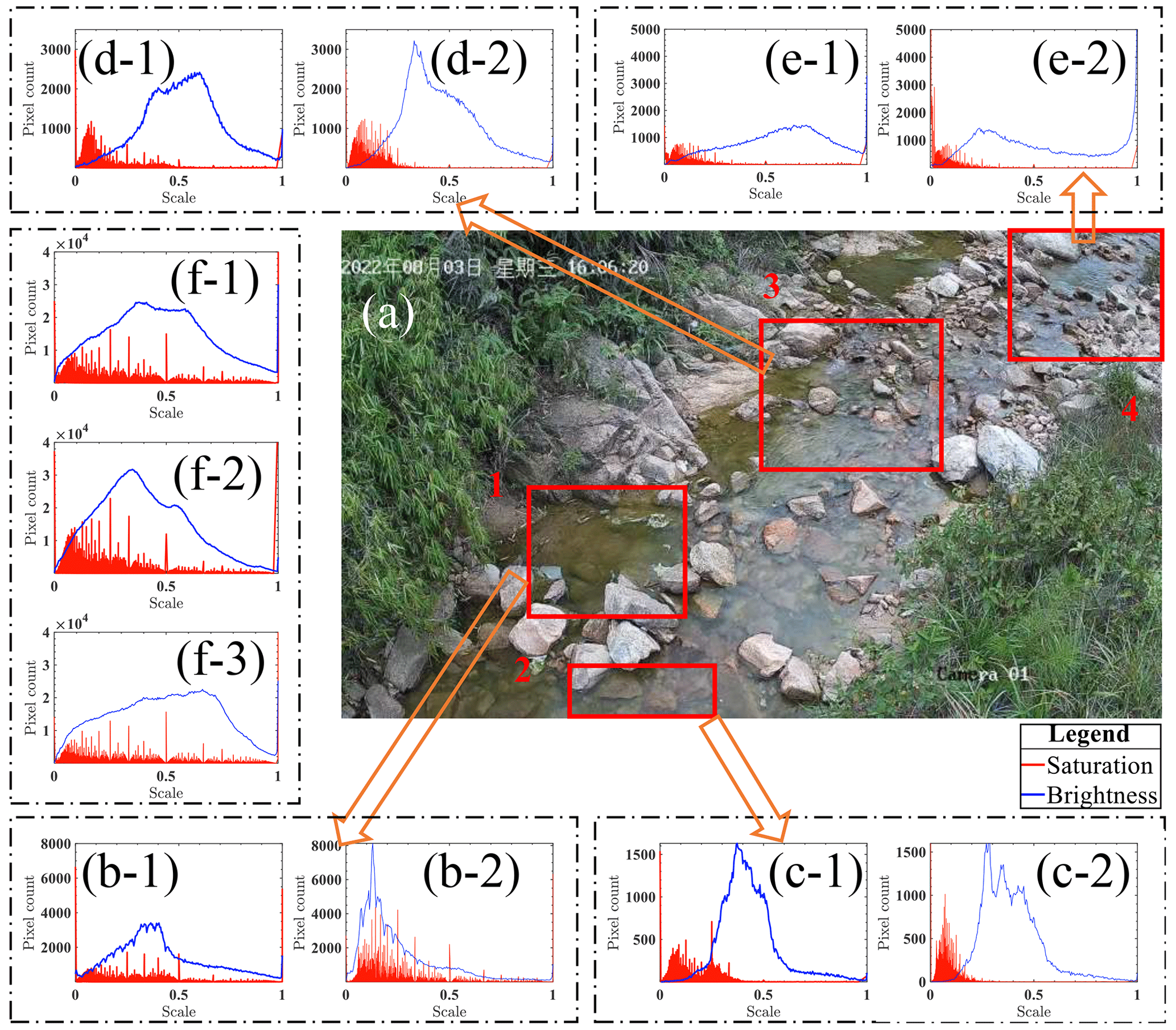
Figure 4 Comparison of saturation and brightness distributions in the four detection areas under different environmental conditions. The horizontal axis is the interval range (0–1) of saturation and brightness in HSB (hue, saturation, brightness) space. The vertical axis indicates the number of pixels under a certain saturation or brightness value. Panels (b-1), (c-1), (d-1), and (e-1) display the saturation and brightness distributions in Areas 1–4 of a good quality sample. Panels (b-2), (c-2), (d-2), and (e-2) display the results derived from samples of below shadow (b-2, c-2), middle shadow (d-2), and water reflection (e-2), respectively. Panels (f-1), (f-2), and (f-3) display the saturation and brightness distributions of an entire image, derived from good quality, dark, and raindrops samples, respectively.

2.3.2 Color enhancement

In order to highlight the stream features embedded in the images and avoid image information redundancy, we compared three commonly used color enhancement approaches to process the image samples.

1. Color-enhanced approach. A dynamic histogram equalization technique (Abdullah-Al-Wadud et al., 2007; Cheng and Shi, 2004) was used to enhance contrast and emphasize stream features. First, vegetation areas on both sides of the stream were cropped and filled in with the color black. Then, histogram equalization was used to enhance the contrast between light and dark, i.e., brighten the bubbles, swirls, ripples, splashes, water coverage, etc. and darken the bottom stones and reflections in the water.

2. Binarization. Binarization of image information can decrease the computational load and enable the utilization of simplified methods compared to 256 levels of grayscale or RGB color information (Finlayson et al., 2002; Sauvola and Pietikäinen, 2000). In this case, the RGB and HSB (hue, saturation, brightness) information extracted from images suggests that the brightness of the stream water under daylight ranges from 0.2 to 0.7 and the values of three color components follow

   $$\begin{array}{}\text{(2)}& R\left(x,y\right)+G\left(x,y\right)+B\left(x,y\right)>\mathrm{350},\end{array}$$

   where R(x,y), G(x,y), and B(x,y), respectively, represent the red, green, and blue color values of the pixel (x,y). The original image was transformed into a binary image by assigning the values of 1 and 0 to the pixels within and out of the waterbody, respectively.

3. Water-color-enhanced approach. Considering that water-color features may carry some useful information on discharge (Kim et al., 2019), we tested a new pre-processing method combining the two approaches above. The RGB information of the original image within the waterbody areas was kept unchanged, while the non-waterbody areas were filled in with the color black. Then, the waterbody areas were further enhanced with the histogram equalization method to highlight the edge transition between the waterbody and the background (Abdullah-Al-Wadud et al., 2007).

2.3.3 Image denoising

Images pre-processed by all three approaches still contain large amounts of noise due to environmental disturbances and edge oversharpening caused by image contrast enhancement (Herzog et al., 2022). Therefore, the wavelet transform (Zhang, 2019) was adopted to denoise the image samples. We chose a compromise threshold between hard and soft thresholds to be the threshold function (Chang et al., 2010). When the wavelet coefficient is greater than or equal to the threshold, a compromise coefficient, α, ranging from 0 to 1 is added before the threshold to achieve a smooth transition from hard to soft thresholds:

$$\begin{array}{}\text{(3)}& {\displaystyle }\mathit{\lambda }={\displaystyle \frac{\mathrm{median}\left(d_j\right(k\left)\right)}{\mathrm{0.6745}}}\times \sqrt{\mathrm{2}\log (M\times N)},\text{(4)}& {\displaystyle }{\mathit{\omega }}_{\mathit{\lambda }}=\left\{\begin{array}{l}\left[\mathrm{sign}\left(\mathit{\omega }\right)\right]\left(\left|\mathit{\omega }\right|-\mathit{\alpha }\mathit{\lambda }\right),\left|\mathit{\omega }\right|\ge \mathit{\lambda },\\ \mathrm{0},\left|\mathit{\omega }\right|\ge \mathit{\lambda },\end{array}\right.\end{array}$$

where j is the scale of wavelet decomposition, d_j(k) is the coefficient of wavelet decomposition, M and N are the length and width of images, ω is the wavelet coefficient, λ is the set threshold, and sign is the sign function. In this case, $M\times N=\mathrm{2560}\times \mathrm{1440}$ and α= 0.5.

2.4 Correlation between color information and discharge

The unstructured image data of mountain streams implicitly contain many stream features relevant to discharge, such as the width and depth of streams, the coverage of the water surface, and spatial distributions of flow direction and flow velocity. In this study, we attempted to achieve discharge monitoring by establishing empirical relationships between the RGB color information of the waterbody and the discharge volumes. We first explored the correlation between the combination of R, G, and B values ($a\stackrel{\mathrm{‾}}{R}+b\stackrel{\mathrm{‾}}{G}+c\stackrel{\mathrm{‾}}{B}$, where $\stackrel{\mathrm{‾}}{R}$, $\stackrel{\mathrm{‾}}{G}$, and $\stackrel{\mathrm{‾}}{B}$ are the mean values of red, green, and blue channels of an image, respectively, and a, b, and c are coefficients to be determined) in the region of interest (ROI; see Fig. 2) and the discharge conditions. Spearman's rank correlation coefficient between $a\stackrel{\mathrm{‾}}{R}+b\stackrel{\mathrm{‾}}{G}+c\stackrel{\mathrm{‾}}{B}$ and discharge is calculated as follows:

$$\begin{array}{}\text{(5)}& r_s=\mathrm{1}-{\displaystyle \frac{\mathrm{6}{\sum }_{i=\mathrm{1}}^n{d}_i^{\mathrm{2}}}{n(n^{\mathrm{2}}-\mathrm{1})}},\end{array}$$

where n is the number of samples, d_i is the difference between the ranks of R, G, and B values and discharge of each image sample.

2.5 Algorithms of discharge estimation

We used three algorithms to establish discharge classification models (Fig. 2), including a convolutional neural network (CNN), support vector machine (SVM), and random forest (RF). The data of the RGB color matrix derived from pre-processed images were used as model inputs. SVM and RF were coupled with CNN to explore the potential merits of traditional machine learning algorithms in improving the classification accuracy and efficiency of CNN-based discharge classifiers. All the embedding image features are normalized and regularized before they are passed to classifiers to avoid overfitting for CNN-based models.

2.5.1 Convolutional neural network (CNN)

A deep convolutional neural network allows computational models composed of multiple processing layers to learn representations of data with multiple levels of abstraction, which have brought breakthroughs in processing images, video, speech, and audio (LeCun et al., 2015). The AlexNet architecture (Krizhevsky et al., 2017) was used to construct our model. The parameters of the semantic layer of the model were calibrated to achieve feature extraction and classification of the stream images. The image size was first rescaled from 2560×1440 to 227×227 to facilitate the migration of trained AlexNet. A $\mathrm{227}\times \mathrm{227}\times \mathrm{3}$ (length × width × color) matrix was retrieved from each image as the model input. There were five built-in convolutional layers using a 3×3 convolution kernel and a 3×3 pooled kernel. We replaced the last three layers of AlexNet with a fully connected layer, a softmax layer, and a classification layer, leaving all other layers intact. The parameters of the fully connected layer were set according to the number of selected discharge values. The rectified linear unit (ReLU) function was used as the convolutional layer activation function to extract and pass on the water coverage features. The softmax function was the activation function of the output layer, and the extracted feature vectors were compressed under each discharge label. The probability that a stream image falls into a discharge label was calculated as follows:

$$\begin{array}{}\text{(6)}& P\left(y\mathrm{|}x\right)={\displaystyle \frac{e^{h(x,y_i)}}{{\sum }_{i=\mathrm{1}}^n{e}^{h(x,y_i)}}},\end{array}$$

where x is the feature vector extracted by CNN, y is the discharge label, n is the number of labels, and h(x,y_i) is the linear connectivity function. The training method for CNN was the stochastic gradient descent with momentum, with 15 samples in small batches, a maximum number of rounds of 10, a validation frequency of three epochs, and an initial learning rate of 0.00005. The samples were shuffled in every epoch. The loss function for discharge classification was cross-entropy loss:

$$\begin{array}{}\text{(7)}& L=-{\displaystyle \frac{\mathrm{1}}{N}}{\sum }_{i=\mathrm{1}}^N{\sum }_{c=\mathrm{1}}^C{y}_{i,c}\log \left(p_{i,c}\right),\end{array}$$

where L is the value of loss, N is the number of samples, C is the number of discharge classes, y_i,c represents the value of the true label for the ith sample in the cth class using one-hot encoding, and p_i,c represents the probability of ith sample belonging to cth class calculated by CNN.

2.5.2 Convolutional neural network coupled with the support vector machine (CNN + SVM)

SVM is a machine learning method based on structural risk minimization and Vapnik–Chervonenkis (VC) dimension theory (Cortes and Vapnik, 1995). It has been widely used in image processing, pattern recognition, fault diagnosis, prediction, and classification (Burges, 1998), which can help to capture key samples and eliminate redundant samples by finding the optimal hyperplane. Compared with neural networks, which rely on large training samples and tend to fall into local optima, SVM can achieve global optima with a simpler model structure (Hanczar et al., 2010; Matykiewicz and Pestian, 2012). However, the SVM-based classifier requires manual input of image features. Therefore, we coupled CNN with SVM to achieve automatic discharge classification. Image features extracted by CNN (i.e., the output of the fifth CNN pooling layer) were fed into SVM classifiers to calculate discharge. The extracted image features coded with a one-versus-all scheme were used to train binary SVM classifiers. Specifically, one SVM classifier with a linear kernel function was trained for each discharge class to distinguish that class from the rest. The hinge loss function was employed to optimize the entire model by maximizing the margin between discharge classes.

2.5.3 Convolutional neural network coupled with random forest (CNN + RF)

RF (Tin Kam, 1995) is a flexible machine learning algorithm that combines the output of multiple decision trees to reach a single result. Each decision tree depends on the values of a random vector sampled independently and with the same distribution for all trees in the forest (Breiman, 2001; Panda et al., 2009). It is an integrated algorithm of the bagging type (Aslam et al., 2007) that combines multiple weaker classifiers, and the final result is obtained by voting or averaging to improve accuracy and generalization performance. Here, we used an RF that comprises 350 decision trees and five decision leaves for discharge calculation. The coupling method of CNN + RF mirrors that of CNN + SVM, with the same pooling outputs for CNN and inputs for the RF discharge classifier. RF is trained to assign optimal weights to each decision tree and leaf without a specific loss function.

2.6 Model evaluation metrics

The performance of discharge classification models was measured by four widely used metrics, including classification accuracy, F1 score, coefficient of determination (R²), and root mean square error (RMSE).

1. Accuracy.

   $$\begin{array}{}\text{(8)}& \mathrm{accuracy}={\displaystyle \frac{{\sum }_{i=\mathrm{1}}^k{\mathrm{TP}}_i}{N}},\end{array}$$

   where TP_i is the number of correctly classified samples in the ith discharge class, N is the total number of samples, and k is the number of discharge classes.

2. F1 score.

   $$\begin{array}{}\text{(9)}& \mathrm{F}\mathrm{1}={\displaystyle \frac{\mathrm{2}\times \mathrm{precision}\times \mathrm{recall}}{\mathrm{precision}+\mathrm{recall}}},\end{array}$$

   where precision is the ratio of true positive classification (TP_i) to the sum of TP_i and the number of misclassified samples with the ith discharge simulated by a model (FP_i) and recall is the ratio of TP_i to the sum of TP_i and the number of misclassified samples with the observed ith discharge (FN_i) calculated as follows:

   $$\begin{array}{}\text{(10)}& {\displaystyle }\mathrm{precision}={\sum }_{i=\mathrm{1}}^k{\displaystyle \frac{n_i}{N}}\times {\displaystyle \frac{{\mathrm{TP}}_i}{{\mathrm{TP}}_i+{\mathrm{FP}}_i}},\text{(11)}& {\displaystyle }\mathrm{recall}={\sum }_{i=\mathrm{1}}^k{\displaystyle \frac{n_i}{N}}\times {\displaystyle \frac{{\mathrm{TP}}_i}{{\mathrm{TP}}_i+{\mathrm{FN}}_i}},\end{array}$$

   where n_i is the number of samples that fall into the ith class.

3. R².

   $$\begin{array}{}\text{(12)}& R^{\mathrm{2}}=\mathrm{1}-{\displaystyle \frac{{\sum }_{j=\mathrm{1}}^N{\left(y_j-{\widehat{y}}_j\right)}^{\mathrm{2}}}{{\sum }_{j=\mathrm{1}}^N{\left(y_j-Y\right)}^{\mathrm{2}}}},\end{array}$$

   where y_j and ${\widehat{y}}_j$ are the observed and simulated discharge, respectively, and Y is the mean discharge.

4. RMSE.

   $$\begin{array}{}\text{(13)}& \mathrm{RMSE}=\sqrt{{\displaystyle \frac{\mathrm{1}}{N}}{\sum }_{j=\mathrm{1}}^N{\left(y_j-{\widehat{y}}_j\right)}^{\mathrm{2}}}\end{array}$$

3 Results

3.1 Correlation analysis

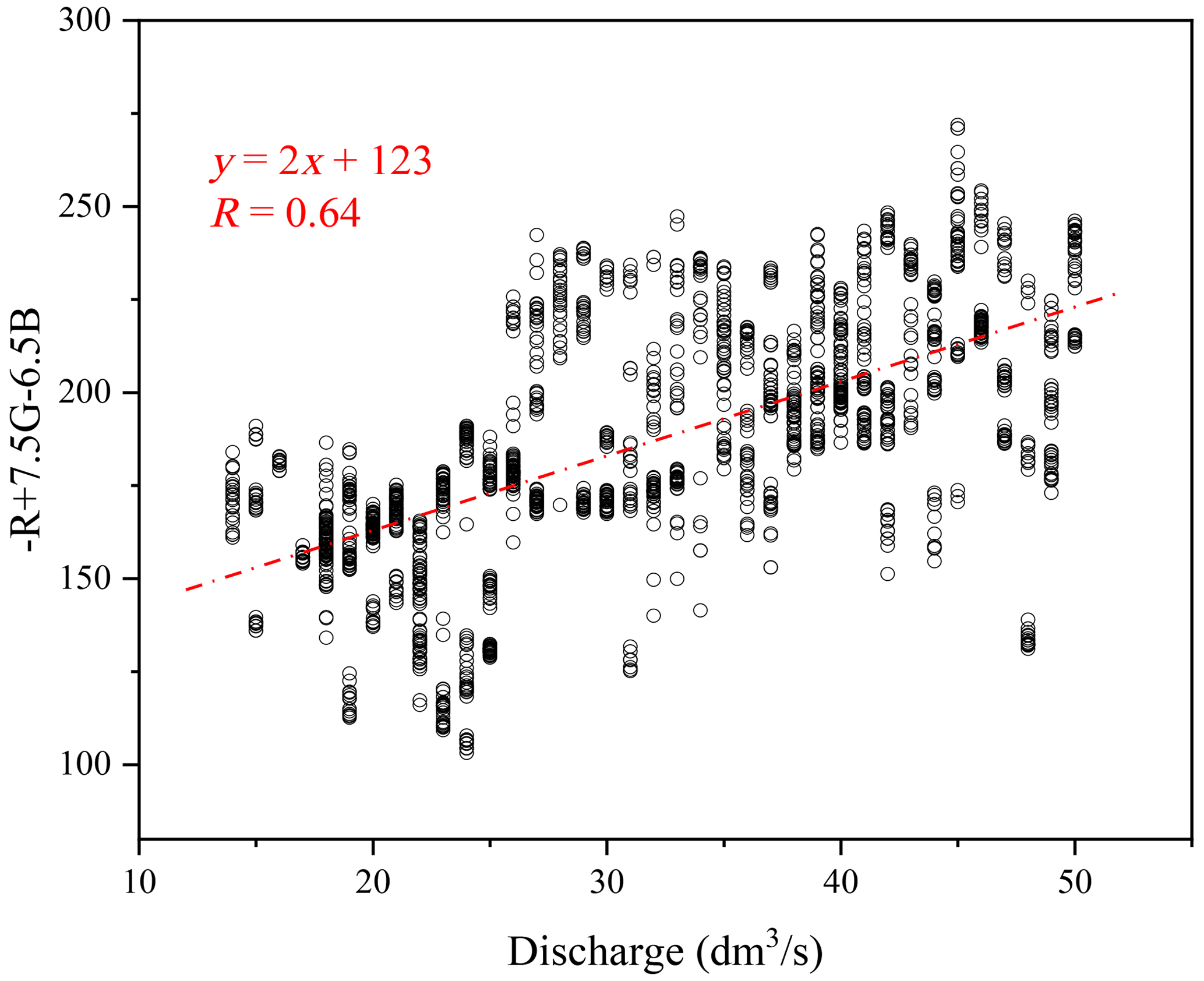
We first performed a preliminary correlation analysis between the RGB matrices in ROI and the discharge values. Traversing the common algebraic combinations of the three colors, we found that $-\stackrel{\mathrm{‾}}{R}+\mathrm{7.5}\stackrel{\mathrm{‾}}{G}-\mathrm{6.5}\stackrel{\mathrm{‾}}{B}$ ($\stackrel{\mathrm{‾}}{R}$, $\stackrel{\mathrm{‾}}{G}$, and $\stackrel{\mathrm{‾}}{B}$ are the mean values of red, green, and blue channels of an image, respectively) had a Spearman correlation coefficient of 0.67 with discharge (p value < 0.01), indicating that the discharge is significantly correlated with the color combination value at the 99 % confidence level (Fig. 5). Such a result suggests that discharge conditions are embedded into RGB information of mountain streams to some extent, which could be further retrieved and refined by CNN models.

Figure 5 Correlation between RGB color values and corresponding discharges.

3.2 Effectiveness of automated image categorization

Most of the previous image-based studies only selected unblemished images for discharge or velocity monitoring, which resulted in poor model performance under environmental disturbances (Leduc et al., 2018; Chapman et al., 2020; Herzog et al., 2022). In this study, we also included samples under the influence of vegetation shadows and water reflection for model training. We selected approximately 100 stream images corresponding to each discharge volume (at the interval of 0.001 m³ s⁻¹) from the pre-processed samples (3168 images in total). The databases of good quality, middle shadow, below shadow, and water reflection were approximately sampled at a ratio of $\mathrm{7}:\mathrm{0.6}:\mathrm{1.4}:\mathrm{1}$ ($\mathrm{2146}:\mathrm{244}:\mathrm{437}:\mathrm{341}$ images) to ensure the representation of different environmental conditions. The samples were distributed evenly in each discharge interval to avoid bias towards particular discharge conditions and enhance model performance for high and low flows (Wang et al., 2023).

Figure 6 demonstrates the difference in classification accuracy of monitoring discharge by the defective images using two sets of models trained with only good quality images and samples filtered by automated image categorization, respectively. Results derived from the three discharge classification models and three color-enhancing methods consistently suggest that the procedure of automated image categorization can significantly improve model performance in apprehending defective images. Classification accuracy of the models trained with only good quality samples staggered between 11.8 % and 18.7 %, while the accuracy of the models trained after automated image categorization was higher than 79.0 % (79.0 %–97.4 %) regardless of the choices of the color-processing method and deep learning model. The average difference in classification accuracy between the two sets of training samples reached 73.9 %. The proportionate inclusion of defective images with vegetation shadow and water surface reflection enhances the anti-interference ability of the models in complex environments.

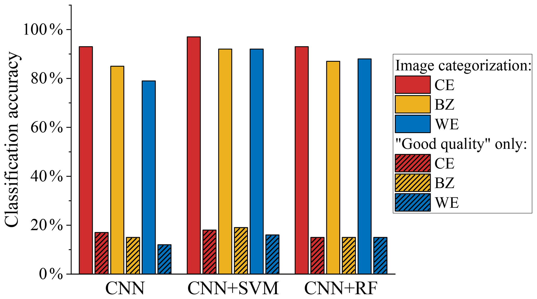
Figure 6 Accuracy of the discharge classification of images under environmental disturbances. Bars with and without patterns show the results using the models trained with only good quality samples and samples after automated image categorization, respectively. Color enhancement methods include color-enhanced (CE), binarization (BZ), and water-color-enhanced (WE) processes.

3.3 Model training and validation

After the treatments of color enhancing, image denoising, and automated image categorization, the images were randomly divided into training and validation sets at a ratio of 7:3 and then used for model training and validation, respectively.

3.3.1 Loss changes

The changes in training and validation loss of the CNN models driven by three types of color-enhanced images are demonstrated in Fig. 7. In the initial 20 epochs, the training loss values decreased rapidly from 7.70 to 3.73 (color-enhanced), from 5.91 to 3.73 (binarization), and from 5.41 to 3.80 (water-color-enhanced), respectively. Subsequently, the decreasing rates slowed during the following 1000 epochs, averaging around −0.0027 to −0.0030 per epoch. The loss value usually stabilizes after 1000 epochs in CNN training (Keskar et al., 2016). In our case, the loss value began to flatten after the 1300th epoch, signifying convergence towards a consistent loss value below 1.00 across all three color-enhancing methods. Therefore, we set the maximum number of training epochs to 1470 to ensure model performance while avoiding overfitting.

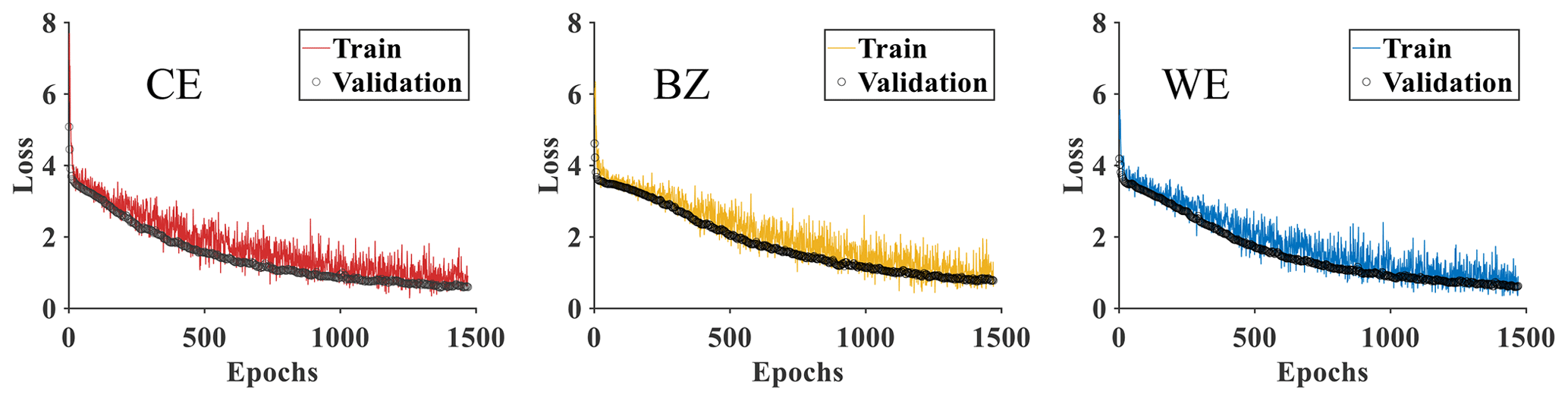
Figure 7 Changes in training and validation loss of the models driven by three types of color-enhanced images. Color enhancement methods include color-enhanced (CE), binarization (BZ), and water-color-enhanced (WE) processes.

The proximity between the training and validation loss changes at the final few epochs is an important indicator that the model is not suffering from overfitting. A commonly acknowledged benchmark of such proximity is approximately 0.1 to 0.2 (Heaton, 2018). In our CNN models, the validation loss values at the final epoch were 0.60, 0.78, and 0.63, respectively, which were 0.19, 0.08, and 0.07 lower than the corresponding training loss. Such results suggest that the models did not suffer from overfitting or underfitting.

3.3.2 Comparison of discharge classification models

The heat map (Fig. 8) visualizes the performance of different models in classifying the validation image set with three tested color-enhancing methods under different environmental conditions. Results show that all three models (i.e., CNN, CNN + SVM, and CNN + RF) can achieve satisfactory performance in discharge classification. The R² under all environmental conditions was greater than 0.97, suggesting that the simulated discharge was significantly correlated to the flowmeters' measurements. The comparison between model performance generally shows consistency under different environmental conditions. Higher classification accuracy and F1 score are always accompanied by higher R² and lower RMSE, showing that CNN-based models perform well in accurately recognizing true discharge and handling outliers. Among the three models, CNN is more likely to over- or under-estimate discharge than both CNN + SVM and CNN + RF, with classification accuracy and F1 score that are 8.6 %–13.4 % and 0.084–0.115 lower than for CNN + SVM and CNN + RF, respectively. With all environmental conditions taken into account, CNN + SVM shows the best overall performance, with the highest classification accuracy of 88.6 %, the highest F1 score of 0.878, the highest R² of 0.989, and the lowest RMSE of 1.08 dm³ s⁻¹. Such results could be related to the size of our samples and the characteristics of the features extracted by deep layers of CNN. The features extracted from stream images under one specific flow discharge show similarities, which highlights the SVM's capability to classify the embeddings from small samples with linear features.

3.3.3 Comparison of color-enhancing methods

Among the three tested color-enhancing methods, the color-enhanced approach generally shows the best performance in discharge classification. Models driven by color-enhanced images achieved higher classification accuracy (+2.3 % to +7.4 %), higher F1 score (+0.033 to +0.067), higher R² (+0.001 to +0.009), and lower RMSE (−0.068 to −0.415 dm³ s⁻¹) than those driven by images processed with binarization and water-color-enhanced approaches. This is partly due to the different treatments in the edges of the waterbody. Binarization and water-color-enhanced approaches cause a relatively larger deviation from the real edges, while color enhanced retains the image information to the maximum extent. Binarization reduces the cost of discharge computation and data storage by transforming raw stream images into binary images and thus facilitates real-time monitoring by embedded end-to-end devices (e.g., mobile phones) with insufficient computing power (Shi et al., 2019). Considering that the color and texture of the water surface vary significantly with discharge volumes while the background is relatively stable, we proposed the water-color-enhanced approach that only processes color information within the waterbody. In our experiment, it only took 0.0154 s to recognize flow discharge from one binarization image with an Intel® Core™ i7-10750H CPU, which was 36 % and 22 % faster than that of Color Enhanced and Water-color Enhanced images, respectively. Such results suggest that it is beneficial to retain the background information to the maximum extent and include the non-water parts of mountain streams in image processing. However, future applications of image-based discharge monitoring need to strike a balance between accuracy and speed when choosing color-processing methods.

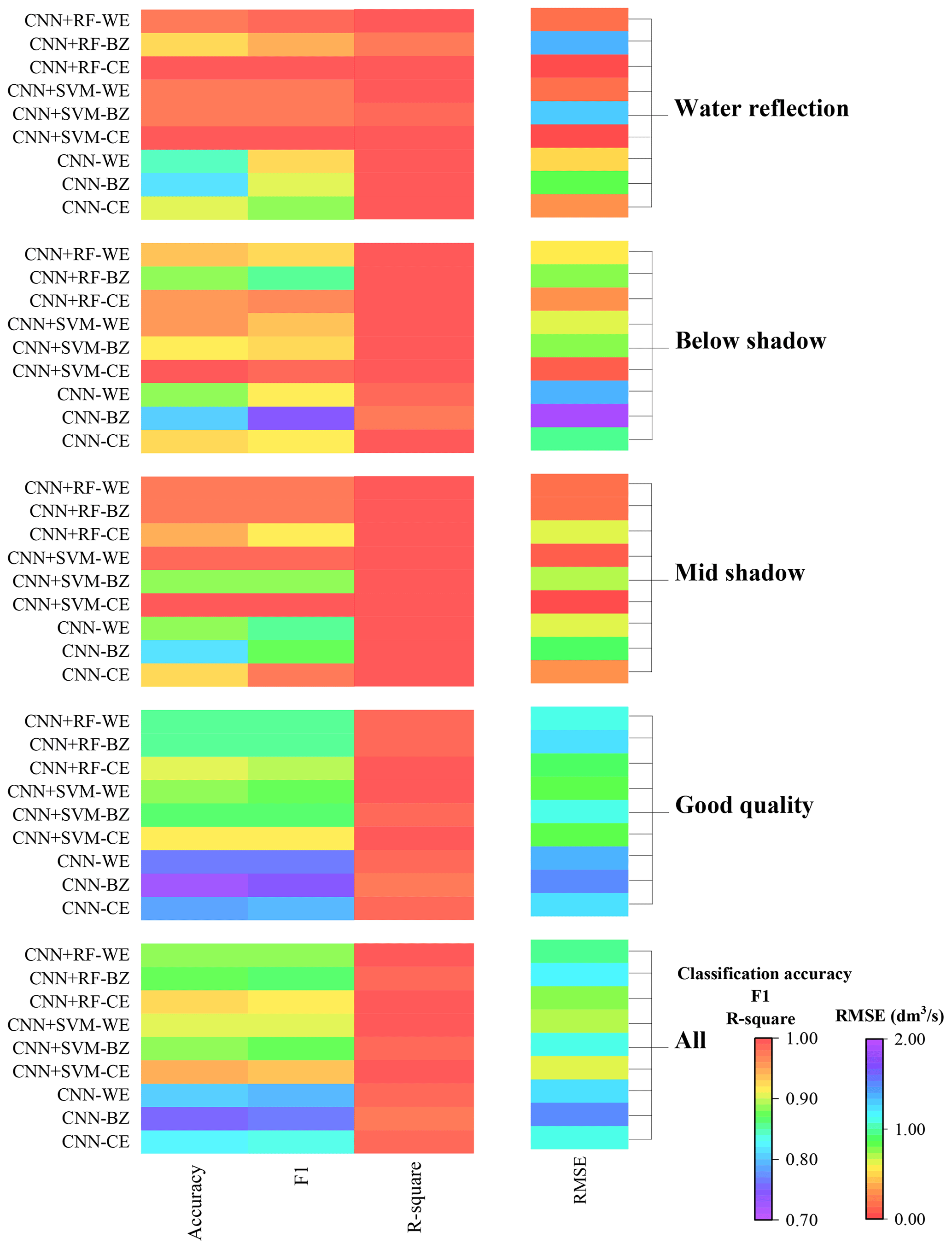
Figure 8 Performance of discharge classification models under different environmental conditions. Color enhancement methods include color-enhanced (CE), binarization (BZ), and water-color-enhanced (WE) processes.

4 Discussion

The existing image-based methods usually rely on either the estimations of flow velocity and cross-section area or assumptions on stage–discharge correlation (Tauro et al., 2017; Leduc et al., 2018; Davids et al., 2019; Li et al., 2019). The first type of method uses image-derived surface velocity to estimate sub-sectional mean streamflow velocity and spatial integration of discharge (Le Coz et al., 2012). The difficulties with capturing cross-sectional characteristics and the relationship between flow velocity and water depth limit their application in small mountain streams. The second type of method retrieves river geometry directly through remote sensing, yet the accuracy is primarily determined by the empirical assumptions about the relationships among water depth, velocity, and discharge (Gleason and Smith, 2014; Young et al., 2015). In this study, we propose a new camera-based method to directly establish the relationship between the RGB matrices of stream images and the classification probabilities of discharge. The unique merit of the CNN-based model is its capability to automatically extract and refine discharge-related features from image samples, which improves the accuracy and applicability of the model. Previous attempts suggest that the selection of image features can significantly affect the performance in the classification of stream images (Tauro et al., 2014). For example, Chapman et al. (2020) manually extracted features from pre- and post-weir images and used them as the inputs for machine learning models. However, the dominant image features related to stream discharge could vary across different environments (e.g., topography, vegetation on river banks, and water quality), limiting the transferability of such manually identified features.

Weather conditions (e.g., sun position, fog, and rain) are the most common difficulties that reduce picture quality (Leduc et al., 2018). Therefore, we designed an automated procedure for categorizing samples by their brightness and saturation: (a) select four areas in the image as detection areas; (b) eliminate images with insufficient light or raindrops on the lens; and (c) identify thresholds and classify the remaining images into four categories for further model training, including the images under the influence of vegetation shadow and overexposure caused by water reflection at certain angles. Such inclusion and categorization of defective samples have significantly enhanced the anti-interference ability of the model, facilitating uninterrupted discharge monitoring throughout the daytime. These factors and the thresholds of brightness and saturation are site-specific and require manual trials to identify them. However, after adequate initial calibration, an established model can be used for the same site for extended periods and repeated installations of camera systems.

The training and validation of deep learning models require a large number of representative samples (He et al., 2016). We collected a total of 7757 image samples from 20 July to 27 September 2022, and 3168 images were used for model training and validation after image screening and categorization. Although we executed an effective automatic categorization procedure on the acquired image samples, it is undeniable that the training and validation sets did not cover all environmental disturbances. For example, the time of sunrise and sunset, the appearance of water surface reflections, and the coverage of vegetation shadows are affected by the angles of sunlight and vary with season. With sufficient artificial lighting or the installation of a night-vision infrared camera (Royem et al., 2012), the images taken during nighttime can also be used for discharge monitoring after training. More image samples are needed to enrich the representativeness of the model in further studies. Another limitation is that we focused on low and average flow conditions in the model training due to the lack of high-quality flood samples. In tropical and subtropical mountain streams of southern China, floods usually occur during rainstorms and only last for a short time. Heavy rainfall constantly blocks the camera lens with raindrops, and the rapid streamflow movement during heavy rainfall tends to cause blurred images, which can only be partly improved by increasing the shutter speed and adjusting the camera position. Moreover, site-specific field data are crucial for identifying the criteria for image categorization and model training, which restricts the broader applicability of our approach in ungauged basins, where such field data may not be readily available. Further research on integrating multiple data sources and surveying approaches is warranted for developing a more generalizable method.

5 Conclusions

This study presents a novel method for discharge monitoring of mountain streams using deep learning techniques and a low-cost solar-powered commercial camera (approximately USD 200). The results confirmed our hypothesis that the discharge-relevant stream features embedded into a large number of RGB images can be implicitly recognized and retrieved by CNN to achieve continuous discharge monitoring. Coupling between CNN and traditional machine learning methods can potentially improve model performance in discharge classification to various extents. In this case, the classification accuracy, F1 score, and R² of CNN + SVM and CNN + RF were 9.1 %–14.4 %, 0.084–0.115, and 0.006–0.010 higher, respectively, while the RMSE was 0.31–0.51 dm³ s⁻¹ lower compared to CNN. Proper image pre-processing and categorization can largely enhance the applicability of image-based discharge monitoring. In an environment under complex disturbances such as mountain streams, image quality is constantly interfered with by shadows of vegetation on the river banks. The automated image categorization procedure can effectively recognize discharge from defective images by filtering samples under different conditions and improving model robustness. The comparison of the three color-enhancing approaches also confirms the importance of including the non-water parts (e.g., large rocks) and retaining the background information to the maximum extent in the image analysis.

The proposed method provides an inexpensive and flexible alternative apparatus for continuous discharge monitoring of rocky upstream mountain streams, where it is challenging to identify the cross-section shape or establish a stable stage–discharge relationship. Site-specific field data are needed to identify the criteria for image categorization and model validation. However, it circumvents the potential errors in assuming cross-section characteristics, such as the relationship between water depth and flow velocity, and represents a new direction for applying deep learning techniques in acquiring high-frequency discharge data through image analysis.