An investigation of anthropogenic influences on hydrologic connectivity using model stress tests

Human influences threaten environmental flows directly or indirectly through groundwater abstraction. In alluvial geological settings, these may affect the contributions from groundwater-sustaining streamflow during dry summer months. The Dreisam River valley in southwest Germany represents a typical case where recurrent hydrological drought events between 2015 and 2022 have led to interruptions of longitudinal connectivity in the stream network. When and where vertical connectivity changes and where the streambed dries out have therefore become important questions. To help answer them, zero water level (ZWL) occurrences were previously measured at 20 locations in the river network during the drought of 2020, but they revealed high variability. This study therefore aimed to develop a methodology that allows the connectivity to be assessed along the entire stream network, i.e. by employing a numerical groundwater model to obtain the spatial distribution of the exchange flow between groundwater and surface water along the river. A reference model simulation for the period 2010–2022 assumed near-natural conditions. Stress test scenario model runs then imposed either an altered recharge regime or a set of introduced groundwater abstraction wells or both. To gain confidence in the model, ZWL patterns are compared to observations of dry riverbed locations in 2020, and the model generally reproduces the observed relative drying. Modelled exchange flows of the stress tests were then compared against the reference simulation. A set of specific metrics combining longitudinal and vertical connectivity is introduced for this task. The results of the stress test model runs show stronger changes of vertical connectivity in response to groundwater (GW) abstraction than to the imposed recharge stress. Reaches are identified where the effects of the stresses are particularly strong. Nevertheless, these results have to be interpreted within the limits of model realism and uncertainty. For more model realism, a number of improvements will be needed such as a higher-resolution parametrization of the riverbed's hydraulic conductivities and better coupling to contributions from hillslopes; for a quantification of the uncertainties, a systematic sensitivity analysis would be required. The study introduces a framework for modelling stress tests and metrics for surface water–groundwater interaction that can be transferred to other cases. It also suggests that even if not all influences can be modelled, the approach may help inform a resilient management of water resources under multiple stresses.

1 Introduction

Expansion and contraction of non-perennial streams cause variations of hydrologic connectivity in space and time in three dimensions: longitudinal (upstream–downstream), vertical (surface–subsurface) and lateral (channel–floodplain) (Datry et al., 2017; Allen et al., 2020; Godsey and Kirchner, 2014; Freeman et al., 2007). The degree of hydrologic connectivity and the direction of the exchange flow control streamflow intermittency and magnitude during dry spells, solute and contaminant transport, and associated nutrient and carbon cycling and consequently also affect water quality and the lotic ecosystem processes (i.e. aquatic biota) (Datry et al., 2017; Costigan et al., 2016; Pringle, 2001). When flow ceases, hydrological connectivity is interrupted, and physical, chemical and biological processes are modified. Notable changes in the frequency and duration of such disruptions of hydrologic connectivity may lead to cascading changes in aquatic ecology. Fluctuations of hydrologic connectivity are particularly severe in non-perennial river systems, where the characterization of spatial and temporal patterns of hydrologic connectivity is important knowledge for water resources management as well as ecosystem conservation success.

While regular or irregular connectivity alternations are the rule in non-perennial streams, it is often challenging to disentangle whether these occur naturally or whether they are due to anthropogenic influences. Water withdrawals from surface water and groundwater are a major cause of hydrological alterations, such as lower flow volumes and prolongation of dry spells in rivers (Yildirim and Aksoy, 2022; AghaKouchak et al., 2021; Goodrich et al., 2018; Datry et al., 2017; Tijdeman et al., 2018). As water withdrawals create fluctuations of the groundwater level and the water stage in streams, they modify vertical connectivity and affect gaining or losing conditions along a stream. These groundwater–surface water interactions may alternate seasonally, depending on the hydrological regime and the hydrogeological setting. Particularly in snow-dominated systems, vertical connectivity becomes more relevant in the summer season, as bank storage is less important (Huntington and Niswonger, 2012). In order to understand if flow alterations in dry phases are exacerbated in response to water withdrawals, it is crucial to investigate the relationship of longitudinal and vertical connectivity.

Many studies have focused on one of the three dimensions of hydrologic connectivity, while fewer studies link the different dimensions of connectivity (Zimmer and McGlynn, 2018). Lateral connectivity studies mostly focus on hillslope connectivity (Zuecco et al., 2019; Blume and van Meerveld, 2015; Rinderer et al., 2019; Jencso et al., 2009) or connectivity of hillslopes to floodplains (Xu et al., 2020; Czuba et al., 2019; Gallardo et al., 2014). Recent studies on non-perennial river systems have predominantly analysed longitudinal connectivity in order to describe flow characteristics (magnitude, frequency, duration) for a characterization of flow regime or to describe the spatio-temporal extent of non-perennial river systems (based on active drainage area, for example) (Price et al., 2021; Hammond et al., 2021; Belemtougri et al., 2021; Botter et al., 2021; Botter and Durighetto, 2020). This one-dimensional perspective with a focus on longitudinal connectivity has also been adopted to investigate whether anthropogenic activities cause hydrological alterations, for example, expressed as “streamflow signatures” for regulated catchments and reservoirs (Salwey et al., 2023; Ruhi et al., 2022; Ferrazzi and Botter, 2019). Statistical models have been used (Jensen et al., 2018) to describe flow dynamics in non-perennial stream reaches, but those models do not consider the physical processes underlying hydrologic connectivity.

Due to a lack of hydrometric data on non-perennial streams at necessary spatial resolution and over longer time periods, another prevalent research goal is the collection of streamflow and water level data at different scales, for example, using field surveys (Zimmer and McGlynn, 2017), citizen science (Etter et al., 2020; Strobl et al., 2020) and new methods to measure dry phases in non-perennial streams (Herzog et al., 2022; Zanetti et al., 2022; Assendelft and van Meerveld, 2019; Jaeger and Olden, 2012).

But without the necessary data, linking the different dimensions of hydrologic connectivity remains difficult (Meerveld et al., 2020).

Specifically for an analysis of vertical connectivity, not only are hydrometric data of the surface water (SW) system required but also data for the groundwater (GW) system. Joint approaches considering GW and SW data are usually restricted by a low spatial data availability of GW heads but also by lacking measurements of transmission losses or GW–SW interaction itself, which are difficult and only possible at particular locations along the stream. Measurement approaches for the quantification of GW–SW interaction are often based on tracers, for example, heat (Angermann et al., 2012; Fleckenstein et al., 2010) or isotopes (Bertrand et al., 2014; Kalbus et al., 2006), which can be used to derive information on flow paths and residence times on very short timescales and small spatial scales only. To date, there is no reliable method for an upscaling of GW data to large scales (Foster and Maxwell, 2018; Barthel and Banzhaf, 2016). Therefore, few data-driven studies on the spatio-temporal evolution of vertical connectivity of non-perennial river systems are documented. Despite acknowledging the relevance of the GW storage term in the water balance (particularly in alluvial aquifers where GW leakage is important) and the retroactive effects between headwater and lower catchment areas caused by GW leakage (Fan, 2019; Käser and Hunkeler, 2016; Covino and McGlynn, 2007), knowledge on the relative roles of the controls of GW–SW interactions remains restricted to few locations.

Given the lack of data, integrated models (IMs) to date have an important alternative role in the investigation of GW–SW dynamics at the catchment scale, even though the possibility for calibration and validation of the simulated GW–SW interaction itself is limited as a result of missing data and required numerical effort (Barthel and Banzhaf, 2016). Uncertainties due to the influence of model resolution on model parameters and the complexity of the parametrization are often discussed as limitations (Foster et al., 2020). IMs have been successfully deployed to obtain a better understanding of the control factors of GW–SW interactions, for example, by means of sensitivity analysis in order to investigate the influence of specific parameters on model results (Herzog et al., 2021a; Foster and Maxwell, 2018) or hypothetical experiments to understand interaction of GW, SW and vegetation (Schilling et al., 2021). However, such experiments are computationally expensive. If obtaining a best-fit model is not the primary aim and interest is more in general responses to changed conditions, targeted stress test model experiments may be a suitable alternative, for example, to assess the response of groundwater drought and baseflow to changed antecedent recharge conditions (Hellwig et al., 2021). Stress test modelling has traditionally been used for management purposes to test the resilience of a system against specific stresses or even worst-case scenarios and has recently been used in applied research in combination with sensitivity analysis. Most of these studies inquire about the effect of different climatic conditions (Hellwig et al., 2021; Stoelzle et al., 2014, 2020), while anthropogenic influences might be equally important in magnitude and relevant for management purposes.

In this study, we develop a modelling framework and specific assessment metrics to examine specifically the alteration of (simulated) longitudinal and vertical connectivity along a stream in response to stresses. These stresses are formalized as a set of model stress test scenarios that employ changes to climatically driven groundwater recharge and to groundwater abstraction and the combination of both. In addition, the aim of the study is to reassess findings from available observations of zero water level (ZWL) for a particularly dry year (Herzog et al., 2022). In this study the longitudinal connectivity was found to be highly variable with upstream to downstream drying in some and the reverse or more complex patterns in other tributaries, but finding clear patterns was hampered by observations at few locations in the stream network. Modelling the entire stream network may enable further insight into spatial and temporal drying patterns, and the observations may help assess the model's ability to simulate stress responses. To analyse the response of the model stress tests to the SW–GW interaction, we introduce metrics that describe the relationship of vertical SW–GW interaction (leakage in modelling terminology) and longitudinal (ZWL) connectivity following general ideas form the hydrological alteration (HA) approach (Poff et al., 2010). We test this stress test approach in a mesoscale catchment in southern Germany, where discussions over streamflow and groundwater uses have emerged during recent dry years with reduced groundwater recharge. In this typical case of an alluvial valley aquifer and locally important river, approaches were needed to inform the debate with multiple water users. The design of the model experiments and stress tests is chosen in order to answer local and more general research questions:

• Do the model experiments confirm the observed relative patterns and spatial distribution of longitudinal and vertical connectivity in the case study area?

• How strong are the responses of connectivity to imposed stresses from recharge deficits and GW withdrawals during a dry summer?

• Can specific metrics distinguish different patterns of longitudinal and vertical connectivity and their responses to those stresses?

2 Methods

2.1 Study area and data availability

The study area is the Dreisam valley (25 km²), a sub-catchment of the Dreisam catchment in the federal state of Baden-Württemberg in southern Germany (577 km²; Fig. 1a). All tributaries have their sources in the Black Forest Mountains and converge in the Dreisam valley, which therefore has gentle slopes in the centre and increasing slopes and altitudes towards the catchment boundaries (Herzog et al., 2022). The geology is characterized by crystalline basement overlain by thick alluvial deposits. The uppermost alluvial materials belong to the so-called Neuenburg formation, younger Quaternary gravels with high hydraulic conductivity (3.2 m d⁻¹). This alluvial filling reaches up to 25–40 m depth in the northern part, whereas it decreases towards the southern part of the study area and contains the main aquifer (Wirsing and Luz, 2007). Older Quaternary sediments with smaller grain sizes below this layer are less transmissive. Previous studies on runoff generation processes suggest that groundwater exfiltration into streams (i.e. “baseflow”) is one of the main runoff processes contributing to streamflow during dry phases in the Dreisam valley (Ott and Uhlenbrook, 2004). However, the degree of the connectivity between groundwater and surface water varies and is difficult to quantify longitudinally.

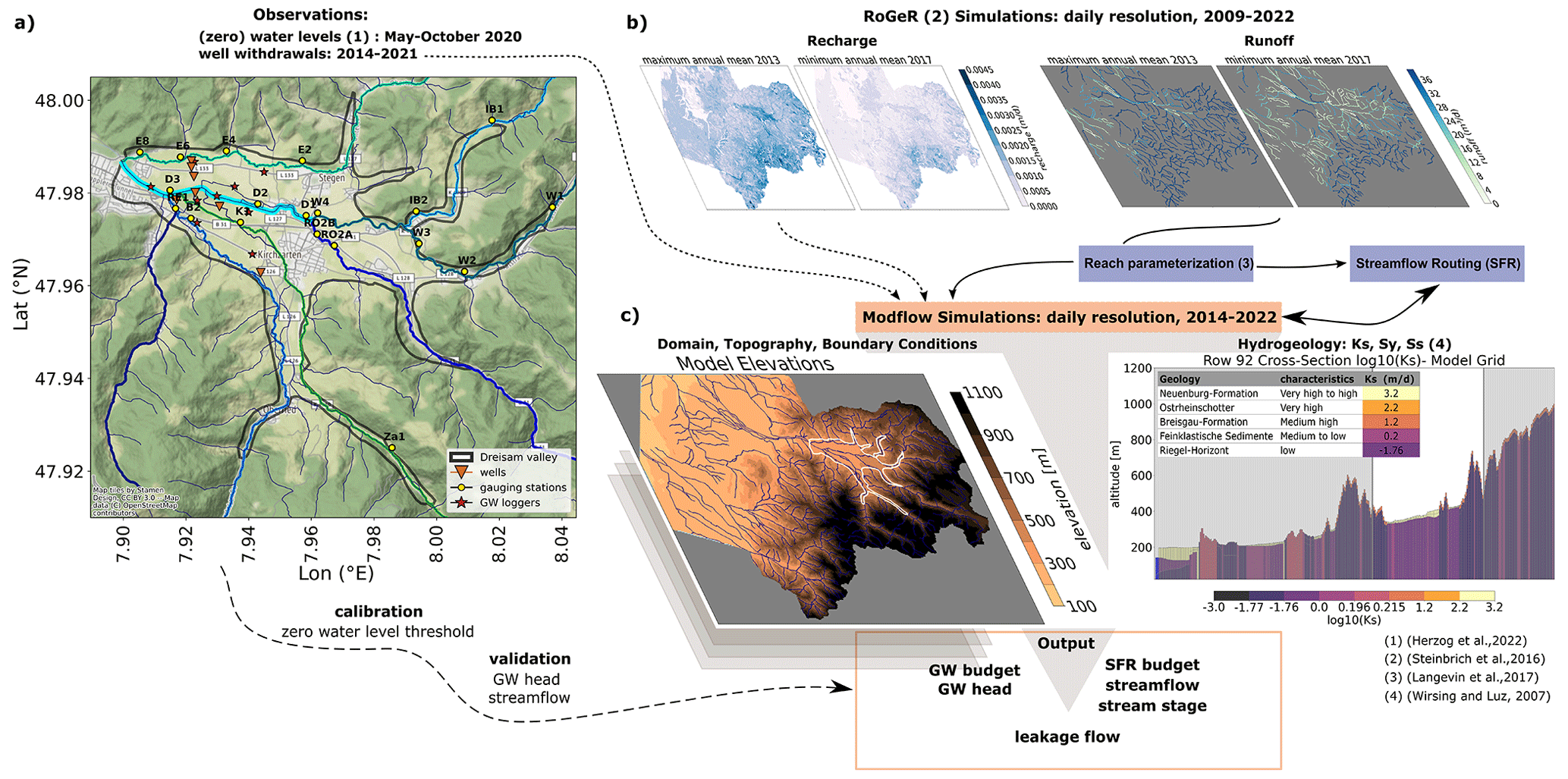
Figure 1 (a) The Dreisam valley with the locations of the gauging stations from Herzog et al. (2022) and the locations of the wells. (b) RoGeR simulation output provides recharge and runoff input to the GW model grid and parametrized river reaches. (c) MODFLOW parametrization based on topography and hydrogeological data. Connections represented as dashed lines denote input that was modified in the stress tests, and bidirectional arrows indicate online coupling.

The aquifer provides about 9×10⁶ m³ yr⁻¹ and half of the drinking water supply of the city of Freiburg im Breisgau. Withdrawals and GW levels are monitored, and data were provided for the period 2014–2022 by the largest regional water supplier (eight locations; see Fig. 1a). Other withdrawals were not available and could not be considered in the model experiment. Based on available public information, however, it is estimated that these withdrawals for water supply account for > 95 % of the total withdrawals in the study area.

Streamflow is monitored by a governmental gauging station at Freiburg-Ebnet, where the valley narrows just upstream of the city of Freiburg. In addition, for the network of surface water tributaries and the main river, a dataset was available containing observed stream stages and ZWL for the summer of 2020, measured at 20 locations in the study area (Herzog et al., 2022). Streamflow measurement campaigns in 2 years with contrasting climatic conditions, i.e. 2020 (dry) and 2021 (wet), were used to develop rating curves for the calculation of streamflow at these ZWL monitoring locations (Herzog and Stahl, 2024). The letters in the station-IDs shown in the figure refer to the different tributaries, i.e. Dreisam (D), Eschbach (E), Rotbach (RO), Wagensteigbach (W), Ibenbach (IB), Reichenbach (RE), Brugga (B), Krummbach (K) and Zastlerbach (Z), of which only those with ZWL in 2020 were used in this study.

2.2 The model concept

To represent both the surface and the subsurface system, we used a combination of the hydrological model RoGeR (Runoff Generation Research Model) (Steinbrich et al., 2021, 2016) and the GW model MODFLOW 6 (Langevin et al., 2017) with surface water routing (SFR package) (Fig. 1). RoGeR is an advanced rainfall–runoff model, which calculates runoff components (interflow, overland runoff, percolation) for unit areas of similar climatic, topographic and pedological properties (version RoGeR WB 1D). MODFLOW 6 solves the three-dimensional, transient GW flow equation (Darcy's law and continuity equation) for the simulation of GW heads. RoGeR and MODFLOW are coupled offline; i.e. the different runoff components modelled by RoGeR are used as input for MODFLOW's stress packages RCH (percolation) and SFR (fast runoff). MODFLOW uses a (block-centred) control-volume-based finite-difference method in order to give an (iterative) approximation of the analytical solution of the partial differential equation. For unconfined conditions (as we assume in this model approach), the transmissivity of a grid cell varies based on saturated thickness of the cell. Detailed information on MODFLOW's modelling approach, as well as the different packages, is given in Langevin et al. (2017).

The model domain not only covers the Dreisam valley upstream of Freiburg but also the entire Dreisam catchment and the neighbouring catchment Möhlin-Neumagen (708.09 km²), with a river network length of 833 km, and the spatial resolution of the GW model is 100×100 m (Fig. 1c). For the model setup, spatially distributed parameters about the surface and subsurface are required. Elevation data were obtained from a 30 m DEM. Four model layers are used in MODFLOW. They were based on subsurface information from gridded data of aquifer thickness, hydraulic conductivity and storativity for each layer of alluvial valley fill according to Wirsing and Luz (2007). The empirical equation of Marotz allows us to determine specific yield as a function of hydraulic conductivity (Fuchs et al., 2017; Marotz, 1968). Time-variable and spatially distributed input to the GW model is then transferred from the RoGeR simulation output and used at daily resolution for the time period of 2009–2022. RoGeR's percolation component, which can also become negative in the case of capillary rise, therefore corresponds to the recharge in MODFLOW. The sum of RoGeR's interflow and overland runoff components corresponds to runoff directly contributing to streamflow. Additionally, transient GW withdrawals are added as groundwater extractions to MODFLOW by means of the WEL package. The regional water supplier provided the required daily pumping rates.

In MODFLOW's SFR package, river reaches are defined as sections of streams in one model grid cell with several parameters such as reach width, depth, slope, thickness, and conductivity of streambed sediments (Langevin et al., 2017). These parameters were derived from topography data, river network data and governmental hydrographic survey data. The simulated GW head in one model grid cell is used to calculate the exchange flow (or leakage) of all the streams corresponding to this particular grid cell. The sign of leakage reflects the groundwater terminology with exfiltrating conditions (negative leakage) describing gaining streams and infiltrating conditions (positive leakage) describing losing streams. The leakage between the aquifer and the riverbed depends on the simulated hydraulic gradient between surface water and GW. For GW heads above the streambed, the gradient is the difference of the stream stage and GW head, whereas for GW heads below the streambed, leakage becomes independent of the GW head, and the gradient is solely the surface water stage above the streambed. Leakage is then calculated as a product of hydraulic conductivity of streambed sediments, the wetted streambed perimeter of the reach and the hydraulic gradient divided by the thickness of streambed sediments (Langevin et al., 2017).

Streamflow for each river reach is obtained based on the principle of continuity, considering that source terms (inflow from upstream reach, direct overland runoff and GW leakage to a reach) equal the sink terms (outflow to downstream reach, diversions from another reach, leakage to the aquifer). Based on this flow, the stream stage is calculated for every reach using Manning's equation. As leakage flow and the overall water budget are dependent on the stream stage, they cannot be directly calculated; the equations need to be solved iteratively.

2.3 Reference simulation and stress test scenario modelling

A reference simulation was needed as a benchmark to compare the stress test simulation results against. Groundwater recharge from the RoGeR model was available for the period of 2009–2022, which was used as input for a transient MODFLOW model run. A near-natural system scenario with this input was chosen as the reference simulation (Fig. 2a) that neglects all water uses in the study area. The case study area has a long history of SW and GW use for a range of purposes, and most of these are not quantitatively known. Only the groundwater withdrawal rates from a main drinking water supplier were available. Other infrastructures include private and smaller groundwater wells, river abstractions for small-scale irrigation, weirs and small-scale hydropower, and trained and stabilized sections of the river for erosion control. Therefore, the model cannot be calibrated or validated to a known natural system state, and the assumption of a natural system scenario is uncertain. Nevertheless this reference simulation can serve as a benchmark to analyse relative changes in stream connectivity in response to specifically applied model stress tests.

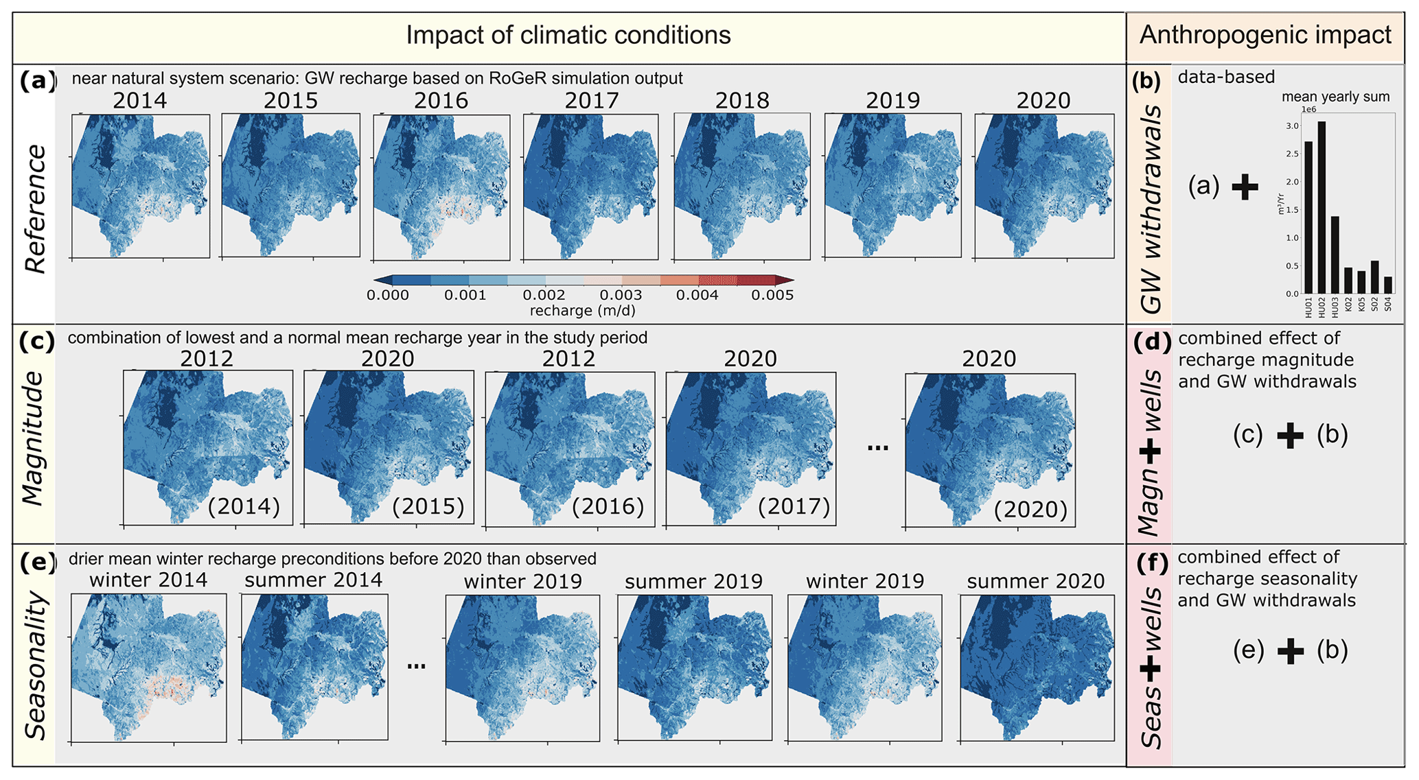
Figure 2 Concept showing all model experiments with the recharge scenarios representing climate stress in the left column, with (a) the reference simulation with real recharge input from 2014–2020, (c) the magnitude stress and (e) the seasonality stress. Anthropogenic impact is in the right column, with (b) expressing the reference with abstractions and (d) and (e) the combined stress of altered recharge and abstractions. For climate impact, the annual mean recharge of the water year or the season is shown. For anthropogenic impact, the mean annual GW withdrawal rates for the period at the wells are shown.

As stress test scenarios, we defined stresses due to the impact of climatic conditions, i.e. by applying altered recharge conditions to the reference model (Fig. 2c and e, left side) and by adding stresses due to the anthropogenic impact in the form of known GW withdrawals (Fig. 2b, d and f, right side) in the valley bottom near the main river. GW recharge is the quantity of water percolating from the surface water system into the GW system and is directly linked to both hydro-meteorological conditions (precipitation and evapotranspiration) and soil properties (infiltration capacity and runoff pathways). According to the RoGeR simulation, the most “normal (average)” water year in terms of groundwater recharge was the year 2012, the lowest annual GW recharge was 2017 and the winter season with the lowest GW recharge was 2019 (Figs. A6 and A7) (a water year starts in November with the summer season starting in May). Synthetic, gridded recharge stress was generated from altering the order of simulated recharge output of the RoGeR model (2009–2022) to create two scenarios: one with changed recharge magnitude (Fig. 2c) and one with changed recharge seasonality (Fig. 2e). Because the dry summer of 2020 was chosen as the main year of analysis, the recharge stress tests focus on changing the recharge conditions preceding 2020. The magnitude scenario focuses on drought stress and therefore replaced the real recharge time series with alternating normal years (2012) and drought years (2020). The seasonality scenario expresses a system change with a tendency for winters to be drier; to simulate this, the driest winter (2019) was repeated again before the summer of 2020. Stress tests of GW water withdrawals are based on real daily abstractions for drinking water that were available for the time period of 2014–2022. The withdrawal stress was added to the reference simulation (for simplicity called “well” scenario) as well as to the magnitude (mag + wells) and seasonal (seas + wells) recharge scenario simulations, allowing a comparison of the system response to altered groundwater recharge, to GW abstractions and to the combination of all stresses.

2.4 Assessment of SW–GW interaction: approach and metrics

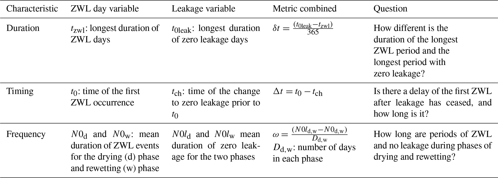
A direct validation of modelled SW–GW interaction is not possible for a number of reasons. None of the model runs includes all human influences on surface water and groundwater in the valley as these have a long history, and quantitative data are unavailable. Therefore there is no simulation that would correspond exactly to the real conditions in the field. Also, exchange rates along the stream cannot be measured continuously in the field. Model grid cells with 100 m resolution will not resolve many smaller stream reach variations that might influence stages and zero flows measured at certain points. Nevertheless, one aim was to test the usefulness of the experimental dataset that exists for the summer of 2020 to build on the insight from a previous experimental study. Therefore the approach is to compare relative patterns and changes of longitudinal and vertical connectivity with specifically developed metrics. For that we were guided by work on the hydrologic regime of non-perennial rivers (Magand et al., 2020; Costigan et al., 2016; Gallart et al., 2012). From an ecohydrological perspective, three (hydrological) aquatic phases (dry, standing, flowing) relate to five (ecological) aquatic states (Meerveld et al., 2020; Datry et al., 2017; Gallart et al., 2017, 2012). The available water level dataset of Herzog et al. (2022) contains derived ZWL occurrences and, thus, the dry phase. The occurrence of ZWL is therefore an indicator for a loss of longitudinal connectivity. Indicators for vertical connectivity are the direction and amount of GW–SW exchange flow (“leakage” in MODFLOW terminology).

Some data prepossessing along with the selection of suitable locations out of the available 20 observational records was necessary to derive ZWL and leakage indicators. For this study, the raw dataset of observed ZWL occurrences (15 min resolution) was converted to ZWL days, respecting a maximum duration (< 24 h) between two ZWL occurrences. In the simulations, negative outliers of simulated stream stages may occur for simulated GW heads far below the surface. We first determined a range of possible zero water level thresholds T for each observational location x within the sum of minimum water level and 5 % (or 1 % depending on the variability) of the mean and the 90 % quantile (Eq. 1) of water levels h at this station.

$$\begin{array}{}\text{(1)}& min\left(h\right)+\mathrm{0.05}\cdot \left({\displaystyle \frac{\mathrm{1}}{n}}\sum _{i=i}^n{h}_i\right)\le T_x\le Q_{\mathrm{90}}\end{array}$$

We then chose the threshold with the smallest difference in the total number of observed and simulated ZWL days. For the locations where ZWL days calibrated this way are comparable with the observations, we assume that the drying phases are well represented by the model and select this subset of “trusted” locations for further metrics and comparisons among the different model runs. The direction (and quantity) of the modelled vertical connectivity of a stream reach can change with time depending on the flow conditions in the stream and the GW head. We assume that the connection between GW and the streambed is lost at first when GW leakage changes to zero. Thus, we extracted direction changes to zero leakage and compare simulated zero leakage and the measured ZWL days. As for ZWL, the definition of zero leakage also requires the use of a location-specific threshold T_leak. We define T_leak as 10 % of the maximum leakage simulated at each location.

In order to analyse the effect of the imposed model stresses, we developed questions regarding vertical connectivity (leakage) and longitudinal connectivity (ZWL). These questions relate to the duration, timing and frequency of the different phases of vertical and longitudinal connectivity (Table 1). For each set of questions, we developed a corresponding metric that allows a quantitative comparison between the model and observations, between reference and stress tests, and among the different stress tests.

Table 1 Metrics for the assessment of connectivity and their underlying questions.

3 Results

3.1 At-site comparison of zero water levels

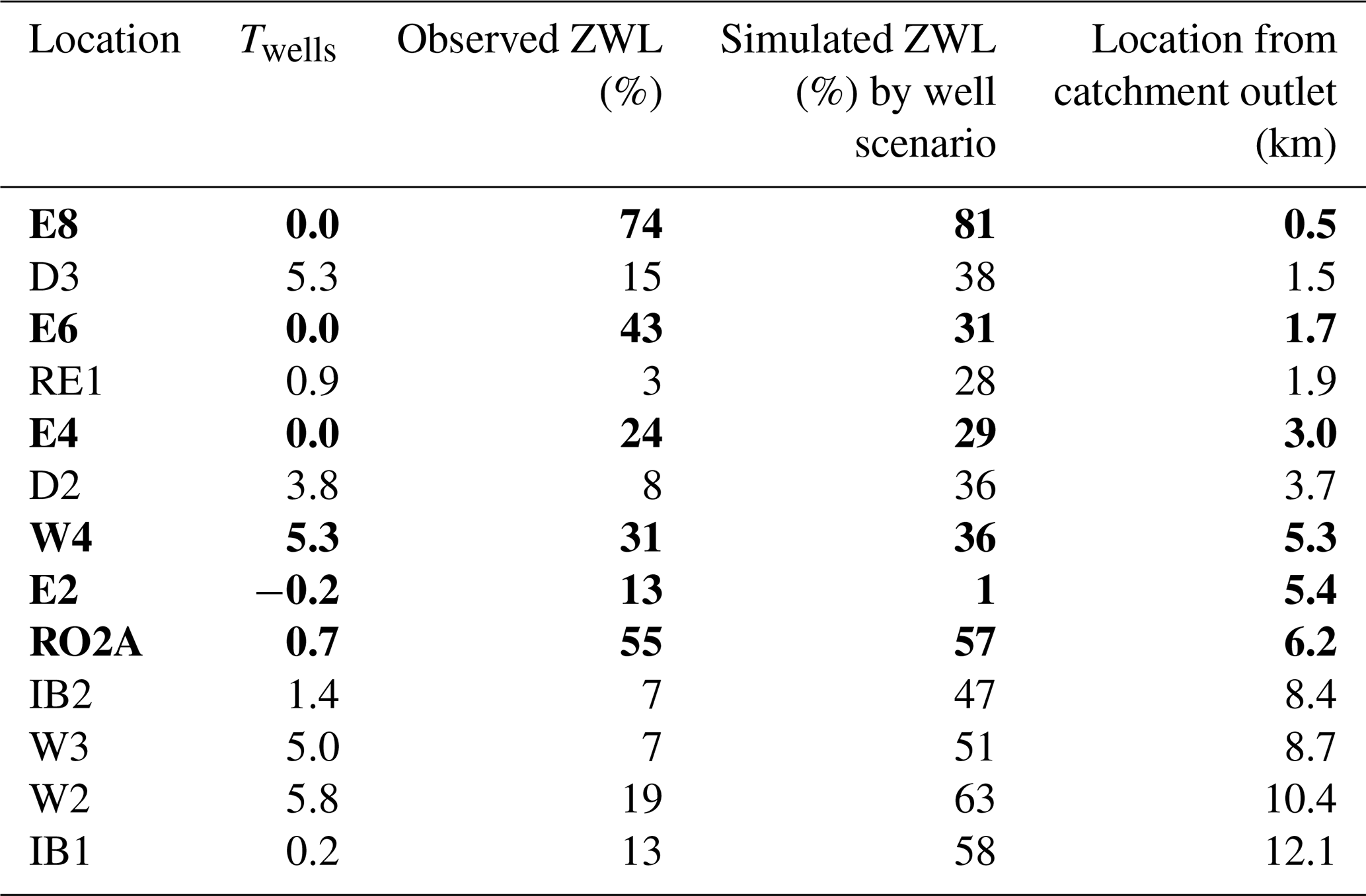
ZWL occurrences were measured at 20 locations in the study area (Herzog et al., 2022). Table 2 shows the ZWL for the well simulation (reference + withdrawals) derived with the help of calibrating the thresholds T. For about 50 % of the locations (E4, W4, RO2A, E6, E8, E2), agreement is good, but for the rest of the locations, differences in ZWL percentage are greater than 15 %. In general, the simulated percentage of ZWL days is higher than for the observations, in particular for locations further upstream, as indicated by the distances from the main gauging station at the downstream outlet of the Dreisam catchment. An exception is the locations E2 and E6. A comparison of mean simulated water levels against observed water levels indicates a general underestimation of water levels in the model despite more heterogeneity in the derived streamflow and an overestimation of mean GW levels (Figs. A2, A1). This disparate bias suggests that the underestimation of water levels is likely due to the streambed parametrization. While the well model simulation should be closest to today's real situation as explained before, it only contains the most important abstractions in the valley. Regarding general relative patterns of ZWL along particular tributaries with three observation locations, the model runs confirm the successively increasing percentage of ZWL from upstream to downstream areas for locations along the Eschbach (E), while the more complex decreasing–increasing–decreasing pattern in the Wagensteigbach is simulated as a consistent decrease. Nevertheless, the two different overall directions are captured by the model run.

Table 2 Derived ZWL day percentages observed and modelled for the study period for two simulations (ordered from upstream to downstream by distance to catchment outlet gauging station, with bold numbers indicating the best correspondence with percentage differences <15% )

3.2 Stress test effects on GW leakage

3.2.1 Spatial distribution of GW leakage in the study area during different GW conditions

The spatial distribution of leakage flow (L) differs for the driest GW conditions (days with highest mean depth to GW) and the wettest GW conditions (days with lowest, simulated mean depth to GW) in the simulation period (Fig. 3). For dry GW conditions the leakage approaches zero, especially in the northern part of the catchment (E tributary) (Fig. 3a and b). In general, the depth to GW is lower in the northeastern part of the catchment. Strong topographic gradients towards the edge of the valley lead to strong hydraulic gradients, which are problematic to represent as an average for one grid cell, and therefore the depth to GW is less reliable in these areas (Fig. A3). Including the abstraction wells in the simulation leads to stronger decrease in leakage in the downstream part of the E tributary (for all stress tests with wells). The recharge scenarios affect the timing of GW drought. The dry GW conditions occur earlier in summer and wet GW conditions earlier in January (at least for the magnitude recharge scenario), but the leakage pattern itself for dry conditions and wet conditions does not differ significantly from reference/near-natural conditions (only if wells are included additionally). For wet GW conditions, the river system is entirely connected to the GW system in the study area as there is almost no place with zero leakage.

The difference in mean leakage (ΔL) of the reference conditions versus stress test conditions shows that the main differences in the downstream part of the catchment are caused by the implementation of wells in the simulation (Fig. 3c). Concerning the magnitude and seasonality recharge scenarios, the ΔL is slightly higher (leakage in the natural system is greater) in the upper part of the E tributary and in the downstream part of the eastern tributaries (towards W and R tributaries). As in Fig. 3a, the effect of wells and modified recharge adds up when both are combined in one stress test. The standard deviation of leakage is highest along the E river, indicating that the variability of leakage is particularly high along this tributary (Fig. 3d). Standard deviation is particularly low at the W and SW borders, where slopes are increasing. However, the abrupt change of the simulated GW head (Fig. A3) suggests that the simulated leakage is highly uncertain here. Nevertheless, the results give a general overview of where in the study area leakage variability and dynamics are particularly strong and more specifically how these changes in leakage are related to physiographic characteristics (such as slopes, topography or whether the location is situated upstream or downstream).

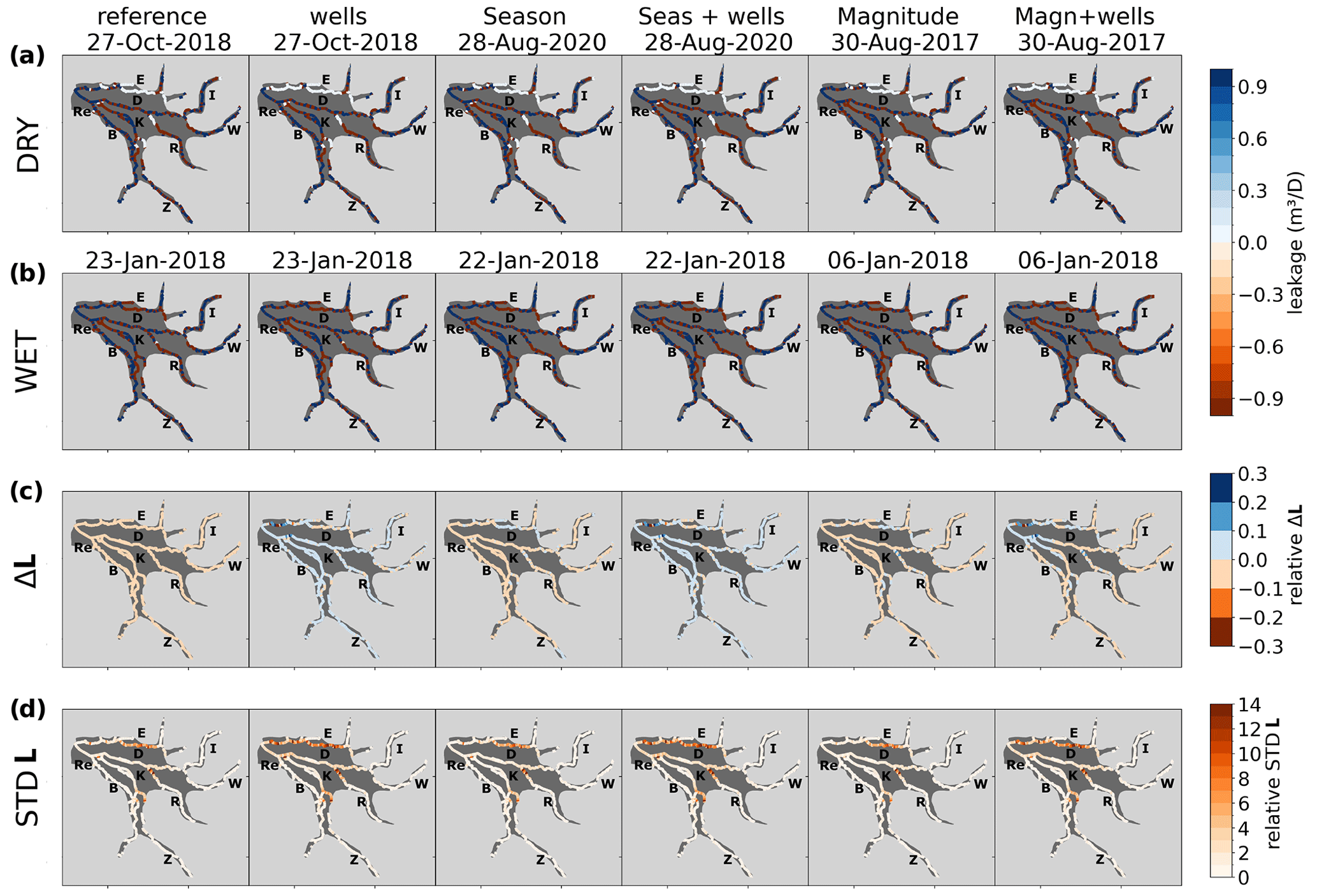
Figure 3 Spatial distribution of leakage in the reference simulation and all stress test simulations, showing (a) wet conditions of mean maximum depth to GW, (b) dry conditions with minimum depth to GW, (c) the relative difference between the stress test simulation and reference simulation, and (d) the relative standard deviation of leakage.

3.2.2 Longitudinal variation of leakage flows

As leakage quantities cannot be validated but depend on simulated stream stage/streamflow, we analyse the longitudinal variation of GW leakage in detail for the different measurement locations in the following. We divided leakage flow by the simulated leakage flow area to obtain specific leakage. For better visualization and comparison, we normalized the leakage flow of 2020, setting the minimum to zero. Minima for the reference simulation and the well scenario are close. Quantities of leakage show strong variations in a longitudinal direction along the riverbed (Fig. 4) and a tendency for decreasing leakage variation with distance from the outlet (IB2, W3, W2, Za1). This pattern however has to be interpreted with caution, particularly due to the overestimation of ZWL days at the stations located far from the outlet. Characteristic of most locations in the main Dreisam river (D3, D2, D1) are losing conditions (from a river perspective). Even though the main gauging station near the outlet (PE) is also located in the main river, it shows gaining conditions. Gaining conditions are otherwise primarily found along the E tributary (E8, E4, E2), except for E6 in the reference simulation. At most locations, there is no profound difference between the reference and the well stress test. The most obvious exceptions are locations in the downstream E tributary (E6, E8 and E4) as well as D3 in the D river.

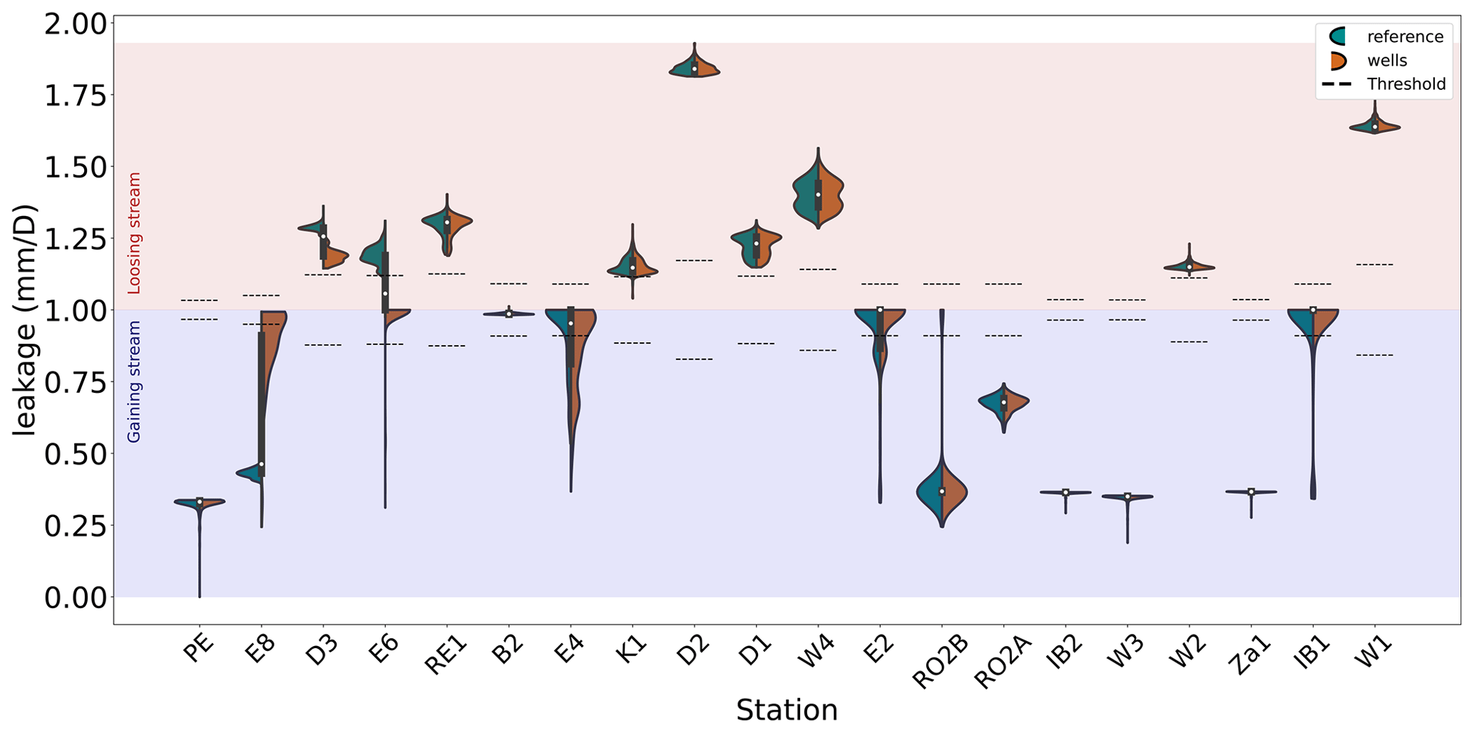
Figure 4 Distribution of normalized specific leakages for the reference scenario and the well scenario for all gauging station locations in 2020. From left to right, the distance from the catchment outlet (station PE) is increasing. Values below 1 (above 1) indicate that the water flow is directed towards the river (the aquifer). Note that thresholds are location-specific, as described in Sect. 2.4.

3.2.3 Comparison of leakage direction changes

In order to understand which stream reaches experience changes from gaining conditions to no connection or losing conditions, we first evaluate the temporal evolution of direction changes at the specific locations for the different stress tests. Three different GW leakage conditions may occur: zero leakage, meaning that there is no exchange between the river and the aquifer; positive leakage (from the perspective of the GW body), meaning that the river experiences losing conditions; and negative leakage, meaning that the river experiences gaining conditions. For normalized leakage, we define zero leakage within a range of $[\mathrm{1}-T_{\mathrm{leak}},\mathrm{1}+T_{\mathrm{leak}}]$, where T_leak is the location-specific threshold (as illustrated by the dashed lines in Fig. 4). For the following analysis, we make a choice of locations based on the occurrence of leakage direction changes first. Note, however, that there are differences in how well ZWL days have been simulated at these locations (Table 2). The characteristics of the temporal evolution of zero leakage and ZWL days form the metrics as described in Sect. 2.4 (Fig. 5). While E8, E4 and E2 experience only direction changes from gaining conditions to zero exchange, E6 experiences direction changes from losing conditions (for natural conditions) to mostly zero exchange (Fig. A5). However, E6 stands out because it is the location closest to the well with the highest abstraction rates, and the flow direction changes differ strongly between stress tests with and without wells. As already noted, the upstream stations along the E tributary experience fewer ZWL days than downstream locations.

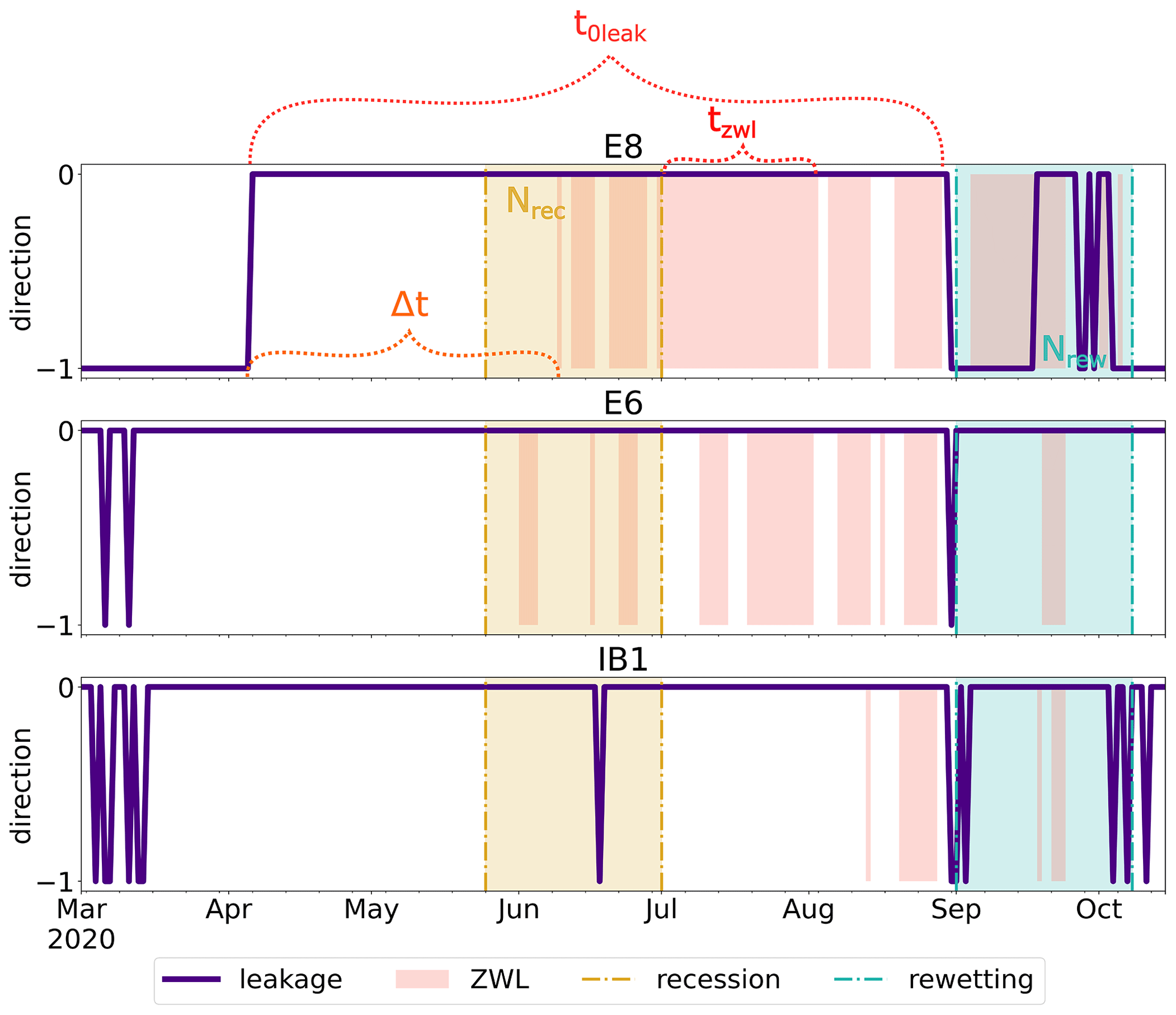
Figure 5 An example of leakage direction changes from gaining conditions (−1) to zero leakage (0) and ZWL days for the well scenario at the measurement locations along the E tributary.

3.3 The relationship of vertical and longitudinal connectivity

For the duration metric δt, values above 0 (below 0) indicate that the duration of the longest zero leakage event t_0leak is greater (smaller) than the duration of the longest zero water level event t_zwl. Mostly, t_0leak is greater than t_zwl (Fig. 6a). For stress tests without wells, the ratio is closer to 0 for E6 and W2. For E8, no zero leakage was simulated in these scenarios. In all stress tests with wells, δt increases, with zero leakage becoming more important at E8 and E6. At E4, δt is more heterogeneous and less influenced by well withdrawals but without a clear response to recharge scenarios either. However, at E2, δt does not vary significantly among scenarios. E2 is also the last station towards the upstream end of the tributary. At IB1, no difference is observed in comparison to the stress tests without wells. δt at W2 and RO2A is more responsive to the recharge stress tests as zero leakage does not occur at these locations in the reference simulation.

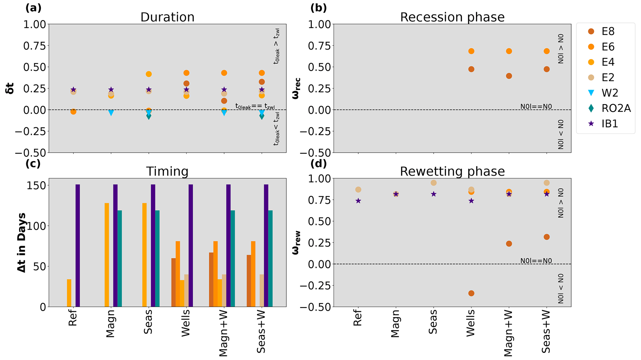
Figure 6 Results of connectivity metrics for the different stress tests at all measurement locations with zero leakage and ZWL days, with (a) duration, (b) frequency during recession phase, (c) timing and (d) frequency during rewetting phase. Dashed lines denote where zero leakage and ZWL days are equally important. For details of the metrics, see Table 1, and for stress test details, see Fig. 2.

The frequency metric ω only differs slightly for the recession and rewetting phases (Fig. 6b and d). For stress tests without wells, almost no zero leakage occurs during the recession and rewetting phase. Thus, it should be noted that the observations do not show ZWL days in the recession phase for some locations. However, at locations such as E8 and E6, where ZWL days occur in the recession phase (Fig. 5), zero leakage already occurs much earlier, and, thus, no ω can be defined. Nevertheless, some differences can be analysed. At E6, ω has the same magnitude for the rewetting and recession phase. At E8, ω is significantly lower, with wells included for the rewetting phase in comparison to the recession phase pointing towards a stronger importance of ZWL days in this phase (as leakage might switch back to gaining conditions earlier). However, the other stress tests with wells show a higher ω during rewetting than during recession. The timing metric, i.e. time delay between first zero leakage and first ZWL day, provides further information about whether ZWL occurs directly in response to zero leakage or not (Fig. 6c). For scenarios without wells, no zero leakage occurred before ZWL in 2020 at all stations except E4 and IB1 in the reference simulation, with Δt being particularly high at IB1. Zero leakage occurs before ZWL at RO2A in the reference and well simulations. In the scenarios with wells, Δt increases for almost all stations (excluding W2). The presence of wells therefore seems to result in a time shift of zero leakage appearing earlier than in the reference simulation and also earlier than ZWL. Interestingly, Δt does not change at E4 for all the stress tests with wells, but it increases for the recharge stress tests. The latter points towards zero leakage occurring earlier under dry recharge conditions. As for δt, Δt at RO2A is only changed by recharge stress tests, but the magnitude of Δt does not change. At W2 no result is found for Δt as there is rarely any zero leakage (Fig. A5).

4 Discussion

4.1 Model evaluation and uncertainties

The application of the complex distributed groundwater model in this study comes with some substantial sources of uncertainty. The model has multiple parameters and processes implemented that can influence the same hydrological variables. Hence, equifinality prevents finding a single “realistic” parametrization. Observational data used for model evaluation are only partially comparable to model output. While data on groundwater heads or surface water levels are point measurements, model outputs integrate flows and processes for the area of the model grid cell. Particularly for high model resolutions and or strong (hydraulic) gradients in one model cell, “correct” model outputs can differ substantially from “correct” observational data taken in the area of that cell. Finally, none of the simulations incorporates all human influences in the stream network and in the groundwater, as noted earlier. As often for complex models such as the model used in this study, computation time hampers an automated formal calibration. Similarly, a sensitivity analysis that might address the parameter uncertainty, ideally based on the full parameter space, so far has not been possible, in part also because if invested, it would also have to include online coupling between the recharge model RoGeR and the MODFLOW model, which again demands resources. Reduced model run times are the main advantage of offline-coupled models (Condon et al., 2021).

As a result of the limitations, differences between observed and simulated ZWL days are substantial at some locations. These differences reflect the simplifications made by the models. Most important to name are the conversion of GW heads from the scale of a grid cell to a river reach unit and the uncertainties in riverbed parametrization. Other studies have illustrated and discussed such difficulties before. Brunner et al. (2010) showed that coarse resolutions of the MODFLOW GW model can lead to underestimation of infiltration in losing streams, which results in a lower GW head and thus also influences streamflow results. Increasing model resolution may reduce this problem (Mehl and Hill, 2010). Strong topographic gradients and coarse resolution do not only impact GW heads but also result in distortion of hydrogeologic properties (Foster et al., 2020; Fleckenstein et al., 2006). This might affect simulated hillslope contributions, which this study did not focus on in great detail. Hillslope contributions that are not correctly represented might explain the poorly modelled ZWL at some of the upstream locations (for example IB1). Additional observations on hillslope connectivity would be necessary to identify where the model misses such inflows into the main tributaries from the headwaters or the hillslopes. In general, future studies may need to assess the influence of spatial resolution on modelled water levels and streamflow (e.g. by decreasing the GW grid cell size) in order to use this model for a quantification of surface water availability. Also, the riverbed parametrization depends on the available raster data, and human structures such as weirs and bridges have not been considered in the parametrization, which may lead to individual affected locations not being represented well. Overall, the spatial discretization of stream reaches likely does not represent the small-scale heterogeneity of streambed. In order to estimate which streambed parameter has the largest influence on the model results, a targeted sensitivity analysis might be helpful. Another option to reduce parametrization errors would be to calibrate hydrodynamic parameters based on hydrodynamic models (Quan et al., 2020) or conceptual models (Meert et al., 2018; Vermuyten et al., 2018) instead of relying on available gridded data. Such additions to the modelling concept were beyond the scope of this study but may present useful extensions in future work.

Model outputs need to be interpreted accordingly, i.e. with these limitations in mind. Simulations at specific locations can be used for relative comparisons but should not directly be compared to real-world observations similar to a validation. The first research question addressed to what degree the model setup would be able to simulate the dynamics or patterns of connectivity and consequentially the riverbed drying in the Dreisam and its tributaries. The question was raised by the experimental zero level data from the dry summer of 2020 that had revealed a high variability in longitudinal connectivity (Herzog et al., 2022). Overall, the model did simulate ZWL days well for locations in the valley bottom, and it distinguished between upstream to downstream increase or decrease in ZWL days in different tributaries. An analysis of longitudinal and vertical connectivity based on the model results allowed us to distinguish between predominantly gaining and losing stream reaches in general to explain these patterns. With the application of stress tests, as is done in this study, the more general and relative system response could be analysed as it is more robust than absolute numeric outputs.

4.2 Response of groundwater–surface water interactions to stress tests

The second research question addressed the response and changes of modelled connectivities in response to the applied stress test scenarios. Despite the uncertainties with respect to simulated system, the model setup provided confidence for the representation of the correct relative responses to changed input or conditions. Following the findings of Hellwig et al. (2021), who found that baseflow reacts on shorter timescales to intensified drought events (especially in fast reacting systems), one would have expected drier recharge preconditions to modify leakage flow. In the stress test simulations, recharge stress mimicking the exacerbation of climatic situations did not respond very strongly, neither for dry nor for wet GW conditions compared to the reference simulation (Fig. 3). Leakage responses were highest for dry GW conditions and the stress tests with direct water abstractions – although with variability among locations. Nevertheless, this suggests that anthropogenic activities exert large influences on GW–SW interaction on such short timescales that may exceed climatic conditions. Locally, this concerns the occurrence of zero leakage in specific parts of the stream network. Therefore, the critical distance to the wells should be further investigated, for example, by means of using stream proximity criteria (Zipper et al., 2019; Li et al., 2022). In our simulations, the well locations and depths were based on observations. However, synthetic stress tests with equally distributed wells and different withdrawal rates could also be envisioned to obtain a general understanding of the impact of water withdrawals. This could help to answer practical questions, such as where GW contributions may buffer the effects of well withdrawals or for the definition of critical withdrawal rates. Critical withdrawal rates could also be investigated, taking seasonality of water withdrawals into account, for example to compare stress tests with more and no water withdrawals in summer.

The stronger impact of well withdrawals on vertical connectivity in comparison to recharge stress may not be valid for longer timescales as GW in particular is a slow-reacting system (Cuthbert et al., 2019). One has to note also that we designed the stress tests to account for current climatic trends of dry recharge years and dry recharge winters to occur more often and not for climatic extremes. We also did not evaluate the effect of longer durations (more than 2 years) of dry recharge conditions, which have been shown to increase the durations of streamflow droughts in rivers from catchments with porous aquifers (Stoelzle et al., 2014). For the two recharge stress scenarios (mag and seas), the interpretation of changes induced by the magnitude scenario is more complex in comparison to the seasonality stress test because the whole recharge sequence was modified.

By evaluating leakage only for the driest and the wettest GW conditions in the study period, we obtain an overview on how leakage differs in the extreme (GW) situation. While this may be particularly relevant for water management, the understanding of how vertical connectivity evolves in response to GW could be improved by an additional event-based analysis (e.g. looking at whole periods of relatively deep (or low) GW heads) or an analysis of the temporal evolution of leakage during changing GW conditions. These synergies between connectivity changes and drought imply furthermore that research on IRES and on drought should not be independent, as elaborated, for example, by Yildirim and Aksoy (2022).

While the influence of recharge stress tests on leakage was low, they did have an impact on the timing of the occurrence of dry GW conditions. With dry winter preconditions in 2020, the driest GW conditions occurred in late August 2020, and with every second year being the driest modelled recharge year between 2009 and 2020, driest GW conditions occurred in late August 2017, as compared to late August 2018 in the reference simulation. On an interannual basis, GW heads were generally lowest at the end of summer, which is in agreement with trends found in other studies based on climate scenarios (Dams et al., 2012). This shift of dry GW conditions due to climatic stress could also lead to a shift in timing of zero leakage in general. However, the timing of dry GW conditions could also be caused by the interplay of different hydrologic variables in specific years, leading to more or less resilience of the GW system to climatic influences. Assessing this further was not the central interest in this study that focused on 2020 due to the available observations. A broadened understanding on vertical connectivity changes due to climatic stress can likely only be achieved through a multi-year analysis of the effects of possible climatic stress tests that are more severe.

4.3 Appraisal of connectivity metrics

The third research question addressed the use of metrics that may help assess vertical and longitudinal connectivities – in models or observations. The metrics as described in Table 1 allow a joint analysis of longitudinal and vertical connectivity that, for example, confirms the impact of water withdrawals in a specific part of the area as in Fig. 3, but they also allow us to demarcate locations that are likely more responsive to climatic (recharge) impacts. The investigation of δt shows that zero leakage persists for longer durations than ZWL for almost all stations (except the ones experiencing very little zero leakage), supporting that ZWL days do not occur independently of zero leakage. δt, Δt and ω along the downstream E tributary stations are influenced by the presence of wells. RO2A and IB1 are most influenced by climatic preconditions, which was shown to have an impact on δt (indicating that zero leakage appears) and Δt (only for RO2A) but not on ω on the other hand. This different behaviour underlines that the relationship of vertical and longitudinal connectivity is very site-specific. W2 and IB1 are both relatively far from the outlet, but IB2 is experiencing a lot and W2 very little zero leakage. These differences can only be expressed looking at multiple temporal characteristics, which highlights the value of the use of such metrics. In this study, zero leakage was mostly found at stations characterized by predominantly gaining conditions (see also Fig. A5). The findings of this study are therefore not necessarily valid for the spatio-temporal relationship between vertical and longitudinal connectivity in losing stream sections. Establishing differences among losing and gaining streams in their connectivity relationship therefore requires more research in different catchment contexts and with larger samples.

Additionally, one also has to be aware of the limits of the metrics due to their definition. First of all, the metrics can only be used for streams experiencing dry spells and zero leakage. The metric for timing could not be calculated if zero leakage does not occur in the same year (stations without bars in Fig. 6c). Considering longer time spans, infinite or very large values would appear for location where the time delay between changes in vertical connectivity and longitudinal connectivity is large. But such large values are difficult to display and imply that there is no link between vertical and longitudinal connectivity changes anyway. Furthermore, the frequency metric is difficult to assess when looking at 1 year only. For a long-term analysis of the evolution of connectivity changes, the frequency metric would serve to compare the recession and rewetting phase in different years. However, this is problematic for analysing intraseasonal differences. The definition of recession and rewetting phase depends on available data (May–November 2020) and the same number of days in each phase but could also be defined differently to actually take into account that each station shows a different drying and rewetting pattern, which does not always happen at the same time during the year. A possibility to adjust the frequency metric to intraseasonal timescales would be to extract the actual recession period at each station based on the hydrograph.

In general, the focus of this study was on understanding the spatio-temporal relationship of leakage flow and ZWL. It could be expanded further, for example, to seasonality if the focus was not only on the summer season. Further metrics might also use leakage quantities (magnitude, rate of change) if sufficient confidence exists in simulated leakage quantities. An analysis of leakage flow quantities will also require more work to obtain the best simulation result.

5 Conclusions

This study presents a model-based approach for assessing the connectivity along the entire stream network and tested metrics on combined longitudinal and vertical connectivity. The Dreisam River valley in southwest Germany that the approach was tested on represents a typical case where recurrent hydrological drought events between 2015 and 2022 have led to interruptions of longitudinal connectivity in the stream network. Employing a numerical groundwater model allowed us to confirm and fill in the knowledge gaps on surface water–groundwater interaction along the river network that had previously been based on a few observations of zero flows. The evaluation of leakage flow for dry and wet GW conditions identifies parts of the catchment where the variability of GW–SW interaction is particularly strong and where GW–SW interaction ceases during dry conditions. This was found for all the model simulations. However, it has to be kept in mind that “natural conditions” with no abstractions and an untrained river system have not existed in this catchment for more than 50 years. Hence, the reference cannot be validated, and the closest integration of human influences only considers a portion of them, i.e. those that are available quantitatively. While confidence was obtained in the model's ability to simulate relative patterns, uncertainties in modelled leakage flows are still high. In order to enhance the soundness of such models, we suggest a broader sensitivity analysis, which includes stress tests, parameter uncertainty and model resolution as a follow-up to our work. However, an analysis of metrics describing the relationship of zero leakage and ZWL (duration, timing and frequency) helped to disentangle the spatio-temporal relationship of zero leakage and ZWL at specific locations. Combined analysis of longitudinal and vertical connectivity is therefore a promising approach. To verify if such metrics are transferable to other contexts, additional case studies in various hydrogeological settings as well as on different spatial scales will be needed. A reference model simulation assumed near-natural conditions. Stress test scenario model runs then imposed either an altered recharge regime or a set of introduced groundwater abstraction wells or both. The stress tests showed that GW withdrawals affect leakage possibly more strongly than the recharge stresses employed. In our study area, well withdrawals influence the intraseasonal relationship of longitudinal and vertical connectivity (duration, timing and frequency) in a way that zero leakage becomes more dominant and, thus, vertical connectivity decreases. Seasonality of the drying may be different for other catchments, which calls for additional studies considering different timescales, in particular seasonal but also annual drying dynamics. Future analysis should also focus on zero flow in addition to ZWL and not only on zero leakage but on all types of leakage directions and on multi-annual datasets. The magnitude of the decrease in vertical connectivity is possibly influenced by the distance to the wells, but in general, our analysis showed that connectivity fluctuations increase and are exacerbated during the recession and rewetting phase in a specific part of the stream network. However, the combined analysis of vertical and longitudinal metrics reveals that the distance from the wells is not the only factor leading to zero leakage. For some locations (particularly upstream ones), climatic preconditions were the primary influencing factor. Overall, this shows the potential of the stress tests to disentangle climatic and human impact. Furthermore, the findings indicate that changes of connectivity patterns in response to different types of stresses might differ depending on the location (upstream or downstream). This could be a starting point for future analysis of such connectivity differences between upstream and downstream locations. Apart from GW withdrawals, other human activities, such as urbanization, soil sealing, land use changes or water withdrawals due to irrigation, can also influence recharge, groundwater heads, and interaction of groundwater and surface water. To assess other factors, model stress test approaches, such as those presented in this study, can be adapted accordingly in the future. For example, the MODFLOW 6 drain package can also be used to implement agricultural drains and other stresses, which potentially modify the GW head. The study introduces a framework for modelling stress tests and metrics for surface water–groundwater interaction that can easily be transferred to similar studies. The application also demonstrates that even if not all influences can be modelled, such studies are useful locally to help inform resilient management of water resources under multiple stresses.

Appendix A

Figure A1 The simulated and observed streamflow and water levels in summer 2020.

Figure A2 The simulated and observed GW heads in summer 2020.

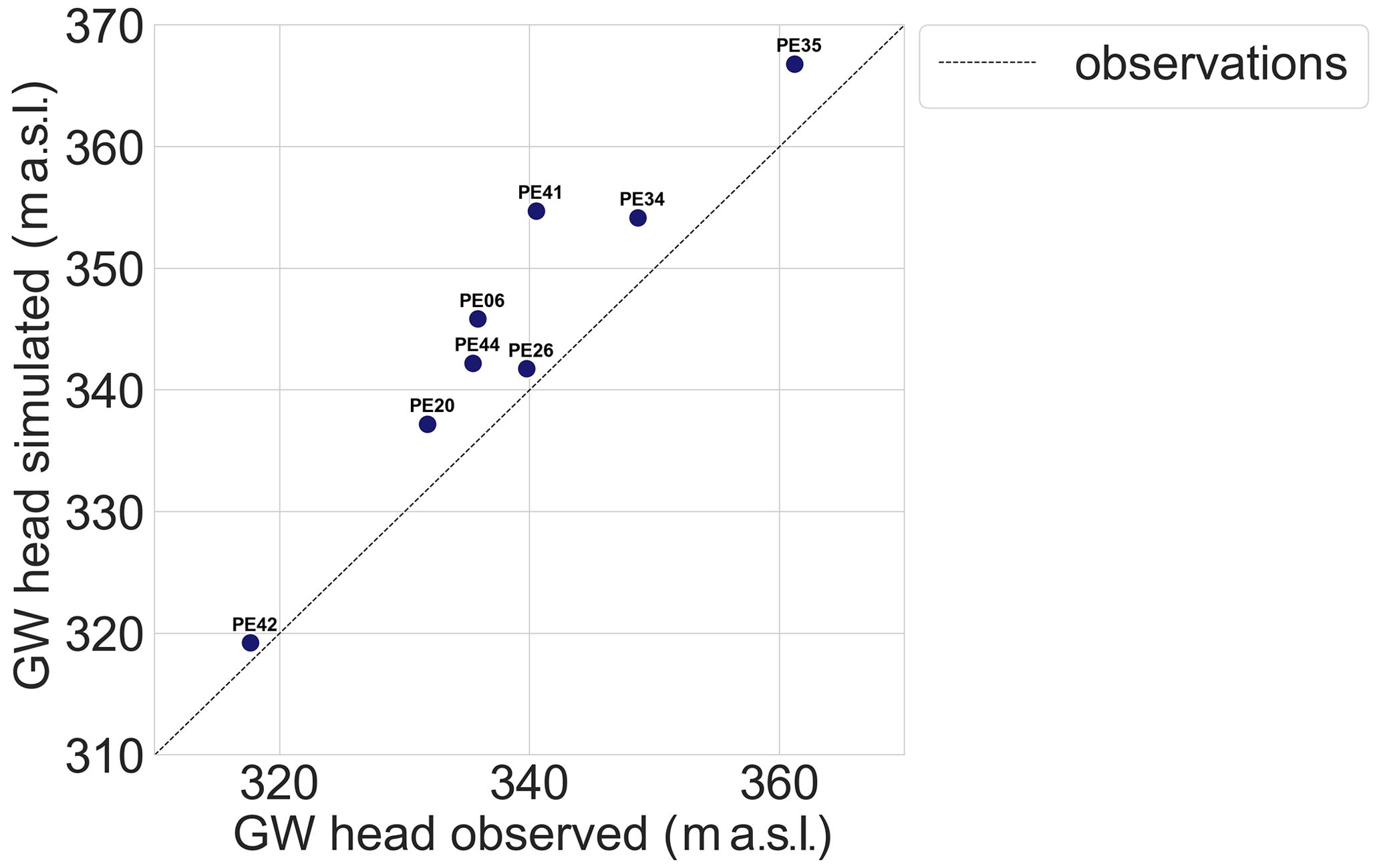
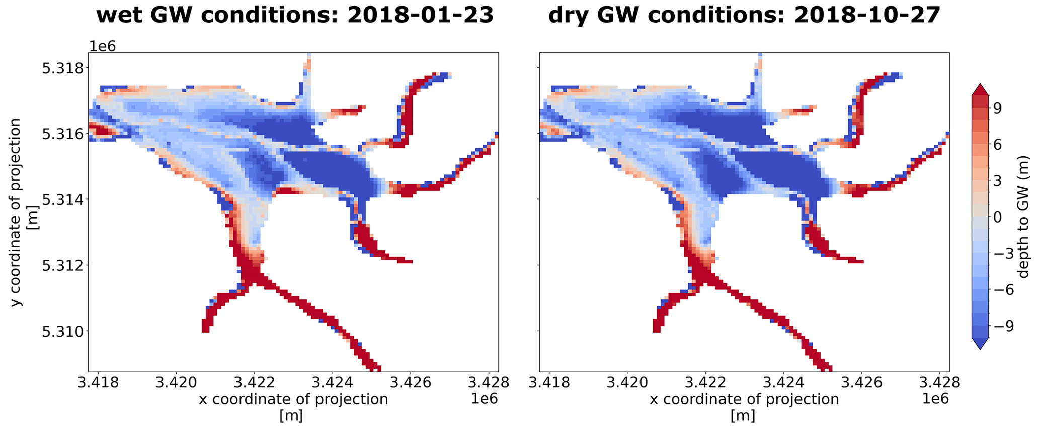
Figure A3 The simulated depth to GW for wettest GW conditions and driest GW conditions in the study period.

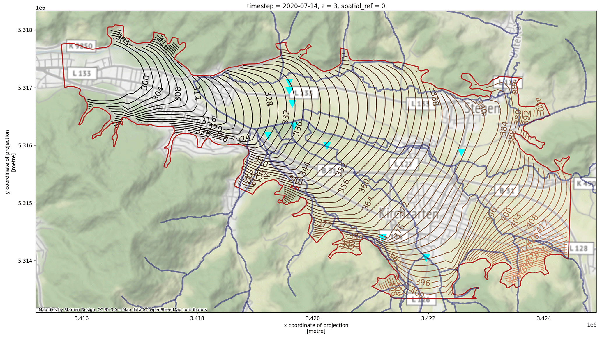
Figure A4 Simulated GW contour lines for the reference simulation for 14 July 2020.

Figure A5 The extracted, normalized direction changes in 2020.

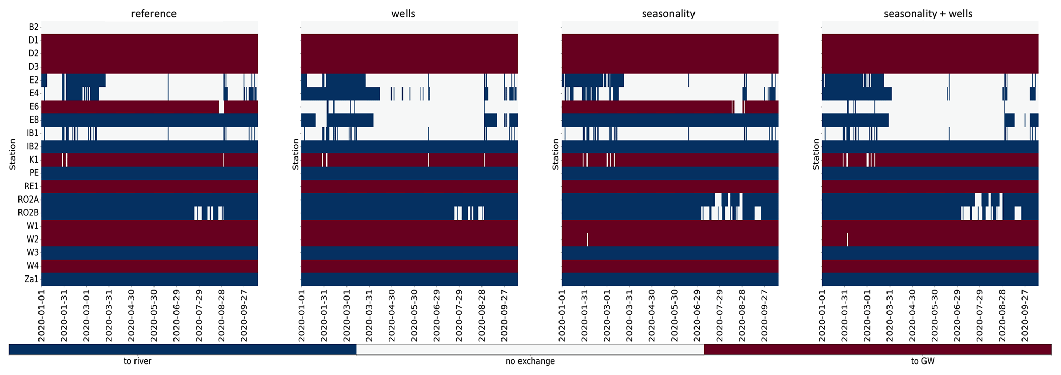
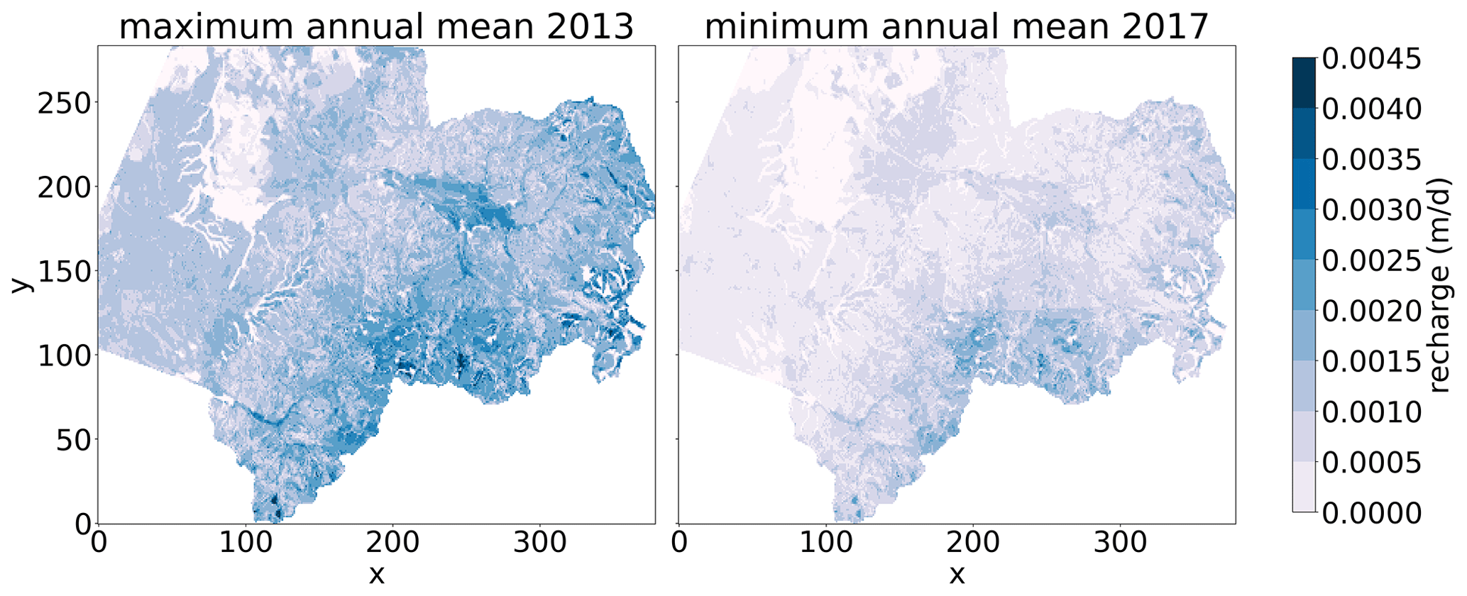
Figure A6 Mean annual minimum and maximum recharge water years for the period between 2009 and 2020 (RoGeR simulations).

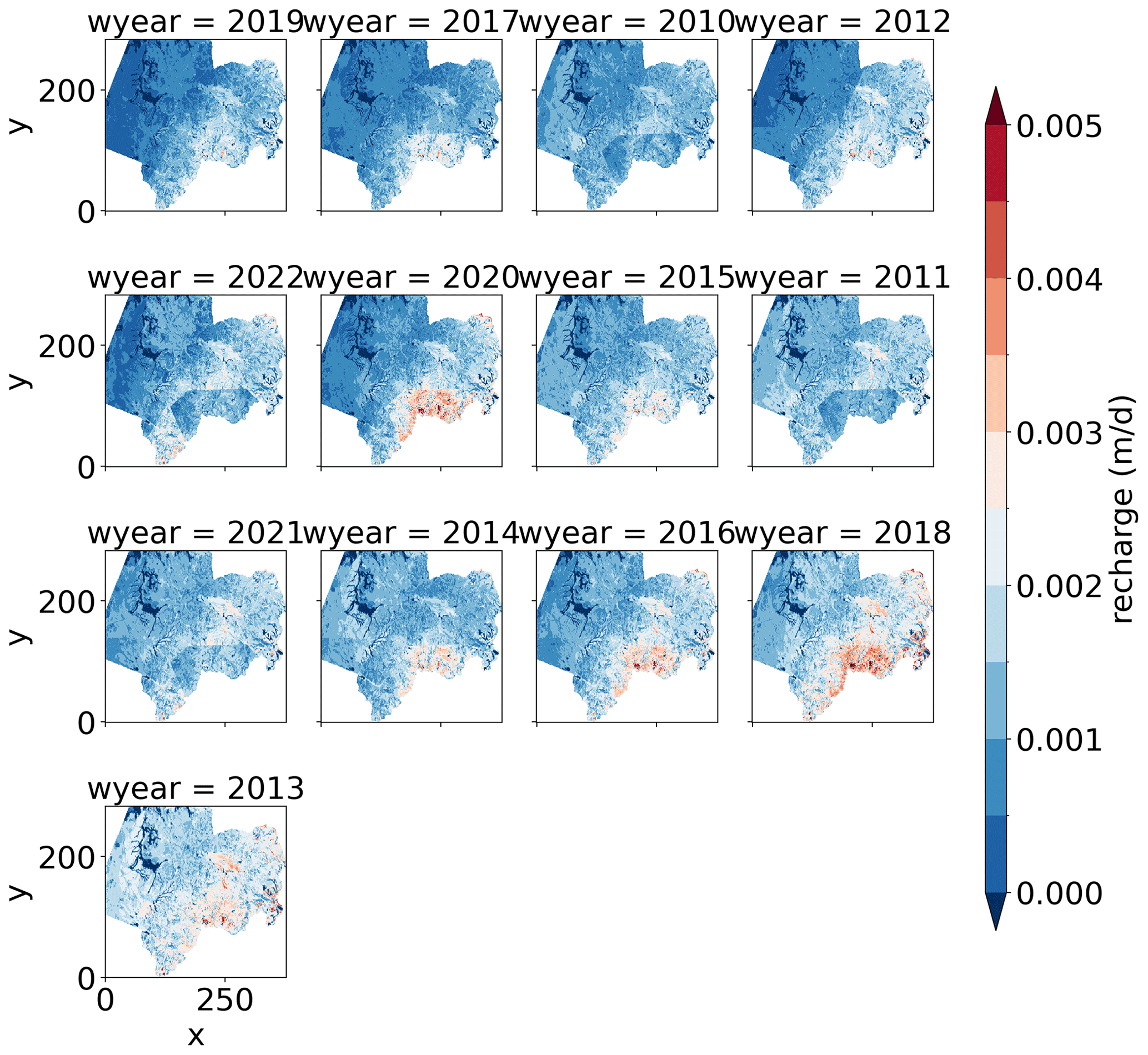
Figure A7 Mean annual recharge for the winter season between 2010 and 2020 (RoGeR simulations).