the Creative Commons Attribution 4.0 License.
the Creative Commons Attribution 4.0 License.
 | 02 Sep 2024
Merging modelled and reported flood impacts in Europe in a combined flood event catalogue for 1950–2020
Dominik Paprotny
Belinda Rhein
Michalis I. Vousdoukas
Paweł Terefenko
Francesco Dottori
Simon Treu
Jakub Śledziowski
Luc Feyen
Heidi Kreibich
Long-term trends in flood losses are regulated by multiple factors including climate variation, demographic dynamics, economic growth, land-use transitions, reservoir construction and flood risk reduction measures. The attribution of those drivers through the use of counterfactual scenarios of hazard, exposure or vulnerability first requires a good representation of historical events, including their location, their intensity and the factual circumstances in which they occurred. Here, we develop a chain of models that is capable of recreating riverine, coastal and compound floods in Europe between 1950 and 2020 that had a potential to cause significant socioeconomic impacts. This factual catalogue of almost 15 000 such events was scrutinized with historical records of flood impacts. We found that at least 10 % of them led to significant socioeconomic impacts (including fatalities) according to available sources. The model chain was able to capture events responsible for 96 % of known impacts contained in the Historical Analysis of Natural Hazards in Europe (HANZE) flood impact database in terms of persons affected and economic losses and for 81 % of fatalities. The dataset enables the study of the drivers of vulnerability and flood adaptation due to a large sample of events with historical impact data. The model chain can be further used to generate counterfactual events, especially those related to climate change and human influence on catchments.
- Article
(9715 KB) - Full-text XML
- BibTeX
- EndNote


Flood risk is constantly evolving and is influenced by a wide array of drivers related to atmospheric, land surface and socioeconomic processes (Merz et al., 2021). Recent decades have been identified as a particularly flood-rich period along European rivers (Blöschl et al., 2020), and increasing sea levels are expected to exacerbate coastal flood risk (Vousdoukas et al., 2017, 2023; Nicholls et al., 2021). At the same time, exposure is growing rapidly (Paprotny et al., 2018b; Andreadis et al., 2022; Rentschler et al., 2023), and mitigation actions are implemented as a reaction to floods (Kreibich et al., 2022). Disentangling the different risk drivers requires considerable modelling effort to reconstruct the factual circumstances surrounding the occurrence of floods and modelling them again under alternative (counterfactual) conditions (Scussolini et al., 2023). Such analyses enable impact attribution, i.e. linking changes in impacts with their likely causes. It can then provide information on the long-term development of risk, which in turn has implications on cost–benefit analyses or risk management planning (Kreibich et al., 2019).
The recent Sixth Assessment Report of the Intergovernmental Panel on Climate Change, in the chapter on Europe (Bednar-Friedl et al., 2022), indicated low confidence in trends in riverine and coastal flood impacts in the past half-century, even if some increase was detected for parts of the continent. The report contained very limited information on attribution, but this gap is being slowly filled by new studies. For example, Sauer et al. (2021) quantified hazard, exposure and vulnerability changes for flood events globally, finding that, for Europe, the increase in flood losses was driven almost entirely by exposure, with a small decline in hazard and vulnerability. Though the time frame of the study was short (1980–2010), it highlighted the role of exposure similarly to Paprotny et al. (2018b), who presented exposure-adjusted losses for 1870–2016 (with consideration of gaps in flood impact reporting), finding no upward trend in economic losses and a strong decline in fatalities. Long-run global data on climatic and socioeconomic drivers under factual and counterfactual scenarios are available from the Inter-Sectoral Model Intercomparison Project, or ISIMIP3a (Frieler et al., 2024), but they mostly have a coarse resolution that is not easily applicable to Europe and have not yet been used for flood impact attribution. Impact attribution of European floods was also carried out with a case-study-based semi-quantitative approach of comparing “paired events”, i.e. floods that have occurred in the same area but some years apart (Kreibich et al., 2023). This approach has an advantage mainly in the context of drawing practical conclusions regarding flood adaptation (Kreibich et al., 2019). Studies that derived projections of future flood risk in Europe have indicated that all three components of risk play an important role in determining changes in the magnitude of impact (Rojas et al., 2013; Vousdoukas et al., 2018; Steinhausen et al., 2022; Schoppa et al., 2024).
Particular effort is needed to reconstruct the intensity and spatial footprint of flood events. For instance, the loss normalization study of Paprotny et al. (2018b) used 100-year riverine and coastal flood hazard maps as proxies for impact zones within subnational regions indicated as affected in the Historical Analysis of Natural Hazards in Europe (HANZE) database (Paprotny et al., 2018a). This approach did not include the effect of climate change, human influence on catchments or simply the variation in the return period of different events. There have been attempts to reconstruct past river floods for North America (Wing et al., 2021) or storm surge footprints globally (Enríquez et al., 2020) but none specifically for Europe. Satellite-derived flood footprints can also be linked to impact records, as in Mester et al. (2023), but such datasets only cover a short time frame and do not resolve the problem of generating a counterfactual hazard scenario.
In this study, we develop a modelling chain to generate a factual flood catalogue for 42 European countries covering the period of 1950–2020, which could further be used to run counterfactual scenarios. We only cover the factual scenarios and focus on deriving the best possible reconstruction of past riverine, coastal and compound floods. The main metric of success of the modelling chain is its ability to correctly derive the time, location and intensity of 2037 actual floods contained in the HANZE flood impact database (Paprotny et al., 2023). We further aim at deriving not only the floods that caused significant socioeconomic impacts, but also those that did not happen despite their hydrological extremity due to existing flood protection as this could later be used to quantify the level of European flood protection.
Thanks to the availability of new high-resolution estimates of past population and economic exposure (Paprotny and Mengel, 2023), we narrow down our catalogue of floods to only those with significant socioeconomic impact potential rather than those which were extreme only from a hydrological perspective. This enables its comparison with historical records of flood impacts and classifying the modelled events in accordance with their real-life consequences (or lack thereof). Finally, the focus is on coastal, compound and slow-onset riverine flooding. Flash flood events occurring in small catchments (i.e. with an upstream area of below 100 km2 in size) are not considered in our analysis due to the insufficient resolution of the riverine flood models available for Europe. Furthermore, we explicitly omit urban floods that result from insufficient storm drainage rather than from channel overflow.
The paper provides a short method overview in Sect. 2.1, which is followed by details on the coastal (Sect. 2.2) and riverine (Sect. 2.3) components of the modelling chain brought together for a final flood catalogue compared with historical records (Sect. 2.4). The validation of the hydrological hazard is provided in the sections that follow (Sects. 2.5 and 3.1), with an overview of risk indicators derived from the catalogue (Sect. 3.2) and, finally, a comparison between modelled and observed flood impacts (Sect. 3.3). The discussion analyses the limitations and uncertainties in both the modelled (Sect. 4.1) and observational data (Sect. 4.2) before drawing conclusions and highlighting possible applications of the flood catalogue (Sect. 5).
2.1 Overview
Simulating riverine and coastal floods requires different modelling approaches. First, we derive extreme river discharges and coastal water levels; we then apply a common approach to produce flood intensity maps, compute damages and spatiotemporally aggregate the results. Compound floods are generated by combining the results of the two strands of modelling work; therefore, we run the coastal model first, and compound floods are considered to be part of the riverine component, drawing on the previous coastal results. The methodology is briefly summarized in Fig. 1.
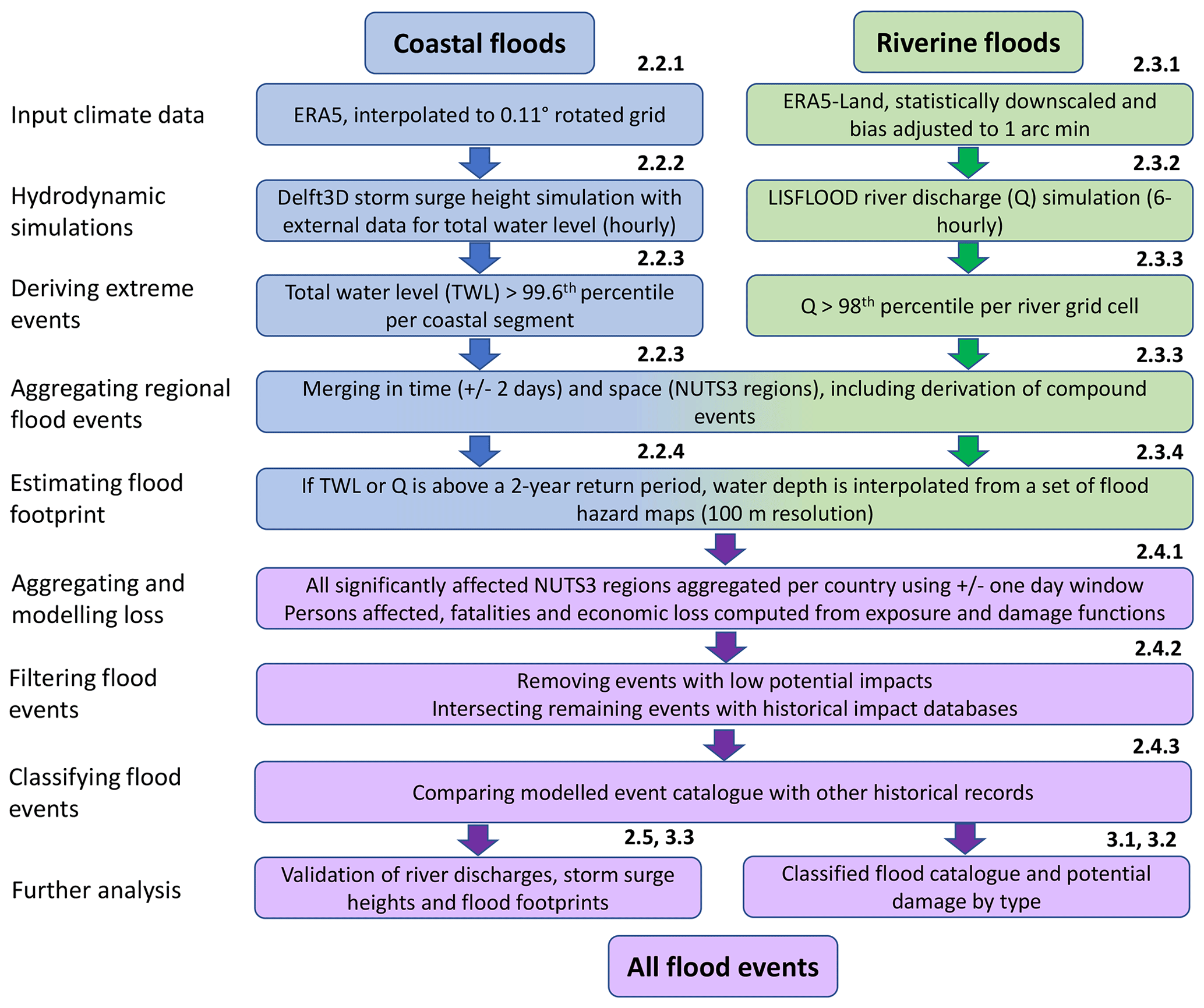
Figure 1Workflow of the methodology, with sections where more information can be found indicated above each box.
In Fig. 1, the spatial aggregation of extreme discharge or water levels using NUTS3 regions is mentioned. This refers to the European Union's (EU) Nomenclature of Territorial Units for Statistics (NUTS). This classification has four levels (0, 1, 2, 3), in which 0 is the national level and 3 is the finest sub-regional division. NUTS3 regions are usually administrative divisions, though at times statistical (analytical) regions are used instead by amalgamating smaller administrative units (Eurostat, 2022). Due to its relevance for determining regional policy, data dissemination and socioeconomic analyses in the EU, we use this classification as our principal unit of analysis. This further enables a direct comparison with the HANZE flood impact catalogue, which contains data on 2037 reported floods in the study area since 1950, including footprints defined at the NUTS3 level (Paprotny et al., 2023). HANZE also includes exposure and other subnational statistics at the same resolution (Paprotny and Mengel, 2023). The generation of a high-resolution boundary map of 1422 NUTS3 regions, as of version 2010, or their equivalents is described in Paprotny and Mengel (2023). We further aggregate flood events at the national level for comparison with reported impacts as this is the typical resolution at which such information is provided. Consequently, the catalogue is not specific for river catchments or sea basins (as in, for example, Diederen et al., 2019) but for countries and their subdivisions.
It should be highlighted that the catalogue represents possible floods without considering structural flood protection measures; hence, they are not included in the potential flood footprint estimates. Due to the very limited information on present or past protection standards, adding estimates of those would potentially create large inaccuracies by filtering out events that happened in history.
2.2 Coastal model
2.2.1 Climate data
We model storm surge heights driven by hourly 10 m wind speeds (u and v component) and surface air pressure, drawing data from the latest ERA5 climate reanalysis (Hersbach et al., 2020). The data were downloaded at a resolution of 0.25° (approximately 28 km at the Equator) and then interpolated using first-order conservative remapping (Jones, 1999) to a 0.11° rotated-pole (12.5 km) grid used in our storm surge model, which in turn is the same as the CORDEX grid used in European climate projections (Jacob et al., 2014). Apart from the interpolation, no further adjustments were made to the data.
2.2.2 Sea level estimation
The principal component of extreme sea levels are storm surges, which we estimate through a continuous simulation in Delft3D. This hydrodynamic model is commonly applied in continental- or global-scale surge modelling (e.g. Vousdoukas et al., 2016a; Ganguli et al., 2020; Muis et al., 2020). The model setup is the same as described in Paprotny et al. (2016, 2019), the difference being that it is forced by wind and atmospheric pressure fields from ERA5 instead of ERA-Interim. We also carried out a calibration using the previous calibration as the starting point by adjusting the sea bottom roughness coefficients for different basins around Europe and comparing the modelled surge heights with tide gauge observations for the years 2011–2019. This recalibration also benefited from much better availability of observational data, which are described in Sect. 2.5, as they are also used to validate the final simulation. Additionally, the time step of the model was reduced to 15 min, with outputs saved hourly, compared to these values being 30 min and 6 h, respectively, in the original version. The model was run from 1 January 1949 to 31 December 2020, with the first year used only as a spin-up. Actual ERA5 data were used in the spin-up phase thanks to recent extension of the dataset to 1940.
As storm surge heights are only one component of extreme sea levels, the hourly total water level (L) is the combination of the following six components:
where S is the hourly storm surge height; T is the hourly tide elevation, computed using the pyTMD package (https://github.com/tsutterley/pyTMD, last access: 20 August 2024) from 34 tidal constituents; W is the hourly wave run-up, assumed to be 20 % of significant wave height (recommended by U.S. Army Corps of Engineers, 2002, and used, for example, in Vousdoukas et al., 2016b); D is the mean dynamic topography, defined as the average sea surface height above geoid for 1993–2012; M is the long-term variation in sea level related to climatic variation (sea level rise, SLR), defined as the average annual difference from the average sea level in year 2000; and G is the glacial isostatic adjustment (GIA) computed from long-term historical rate of change.
Table 1Source of data for computing the hourly total water level. ∗ Coarser global data were used for the northernmost coasts of Europe.
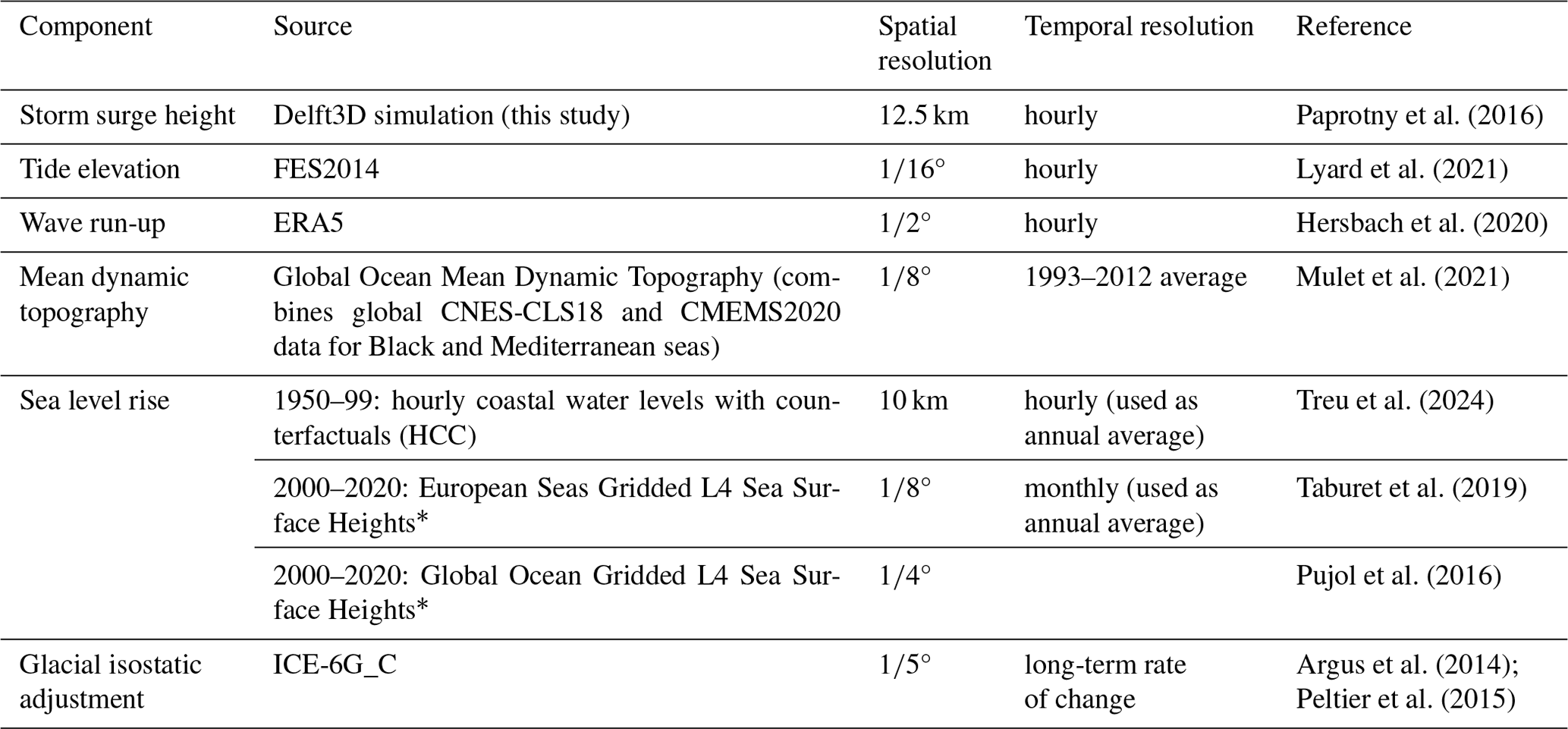
Each component was derived from a different source as summarized in Table 1.
2.2.3 Extracting coastal flood events
As the resolution of each dataset that is used to derive the total water level varies, we assign the nearest grid point of each model to 5884 coastal segments defined in the coastal flood hazard model (Vousdoukas et al., 2016b) using the nearest-neighbour approach. The segments represent no more than 25 km of the coast (if completely straight) but usually about 15 km. They stretch up to 100 km inland, but far less for more complex areas such as deltas, estuaries, fjords or islands. From the detrended (1950–2020) hourly time series, occurrences of water level above the 99.6th percentile were identified and considered potential coastal floods. The detrending was needed as events derived here are used for extreme value analysis (Sect. 2.2.4). The occurrence of water levels below the 99.6th percentile for at least 2 full calendar days separated two events from each other. Such thresholds lead to, on average, about five potential flood events per year. Events were then aggregated according to NUTS3 regional boundaries, again following the principle that the beginning of any segment-level flood event in a NUTS3 region has to occur at least 2 full calendar days after the end of any previous segment-level event in that region.
2.2.4 Deriving coastal flood footprints
For each coastal segment in the dataset, an extreme value analysis was carried out using a generalized Pareto distribution and a peak-over-threshold approach. The analysis was carried out using the MATLAB function fitdist and the maximum likelihood estimation and the 99.6th percentile thresholds from the previous step. This enabled the derivation of extreme sea level scenarios (return periods of 2, 5, 10, 20, 30, 50, 100, 200 and 500 years) for coastal inundation modelling. This was carried out according to a methodology developed by Vousdoukas et al. (2016b). Briefly, the maps were generated using the LISFLOOD-ACC (LFP) model (Bates et al., 2010) that was applied at a 30 m spatial resolution. In terms of digital elevation models (DEMs), we use the recently published GLO-30 DEM (European Space Agency and Sinergise, 2021) after post-processing using global lidar observations to further remove vertical bias, correcting for buildings and vegetation. The description of the GLO-30 post-processing is described in detail in Pronk et al. (2024). The simulations consider gridded hydraulic roughness values derived from land-use maps (Zanaga et al., 2021). LISFLOOD-ACC is applied for each coastal segment, with the model domain extending up to 200 km landward in order to ensure the inclusion of all potentially hydrologically connected areas that may lie inland and away from the coast.
Total water level of each segment-level flood event is linked with the water level used to generate the flood hazard maps for each segment. In this way, it is possible to interpolate water depths from the stack of hazard maps to event-specific extreme sea levels. This is only done if the water levels for an event exceed a flood threshold, defined as the higher of the following two thresholds:
-
total water level with a 2-year return period derived from the generalized Pareto distribution and
-
maximum observed total water level with the storm surge height subtracted.
The first threshold was chosen for consistency with the riverine model as it is akin to the typical definition of a bank-full river discharge. The second threshold was added to avoid overestimating risk in regions (mainly eastern Mediterranean) where storm surge heights are very low but wave run-up contributes significantly to extreme sea level.
Only grid cells with water depths of at least 10 cm were considered inundated for consistency with riverine flood maps. The individual flood maps for each coastal segment were aggregated within a NUTS3-level event. Finally, those NUTS3-level events were only preserved for further analysis if the potential flood zone was at least 100 ha. As further processing is carried out together with the riverine model, we now describe the river component and continue explaining the next steps toward the combined flood catalogue in Sect. 2.4.
2.3 Riverine model
2.3.1 Climate data
We used river discharge from Tilloy et al. (2024) that was modelled using ERA5-Land, which is a downscaled version of ERA5 characterized by a 0.1° (approximately 11 km at the Equator) resolution (Muñoz-Sabater et al., 2021). It was further statistically downscaled and bias-adjusted a to 1′ (arcminute) resolution using ISIMIP3BASD v3.0.0 method developed by Lange (2019, 2022) using European Meteorological Observations (EMO-1) gridded observational data, which are data from a 1′ variant of the EMO-5 dataset developed by Thiemig et al. (2022). Temperature and precipitation at a 6-hourly resolution were used as the primary drivers of the hydrological model, while potential evapotranspiration was computed at a daily resolution using the LISVAP model by van der Knijff (2006). For details on the preparation of the meteorological data, we refer the reader to Tilloy et al. (2024).
2.3.2 River discharge simulation
Tilloy et al. (2024) modelled river discharges a through continuous simulation using the LISFLOOD hydrological model (Burek et al., 2013) implemented in the European Flood Awareness System, or EFAS (Copernicus Emergency Management Service, 2023). Tilloy et al. (2024) used the latest model setup, v5.0 (Choulga et al., 2023), and simulated river discharges with meteorological inputs described in Sect. 2.3.1. The EFAS model was run from 3 January 1950 to 31 December 2020 following the 71-year pre-run. Due to the rapid evolution of socioeconomic conditions in the catchments of Europe, the input socioeconomic maps were changed with the start of every new calendar year of the simulation. The evolving socioeconomic conditions included land use (in six classes), reservoirs (based on the year of construction of each dam) and water demand (in four sectors). For details on the river discharge simulation and its validation, we again refer to Tilloy et al. (2024).
2.3.3 Extracting riverine flood events
From Tilloy et al. (2024), we derived a time series of 6-hourly discharge for 7.5 million grid cells. Due to the availability of flood hazard maps for footprint estimation (Sect. 2.3.4), we extract data only for 282 528 grid cells that have an upstream area of at least 100 km2. Occurrences of discharge above the 98th percentile (on annual basis) were identified and considered potential riverine floods. Occurrence of water levels below the 98th percentile for at least 2 full calendar days separated two events from each other. As in the coastal model (Sect. 2.2.3), those thresholds were intended to produce roughly five potential flood events per year in each grid cell. Events were then aggregated according to NUTS3 regional boundaries, again following the principle that the beginning of any grid-cell-level flood event in a NUTS3 region has to occur at least 2 full calendar days after the end of any previous grid-cell-level event in that region.
2.3.4 Deriving riverine and compound flood footprints
For each grid cell in the dataset, an extreme value analysis was carried out using a generalized Pareto distribution and a peak-over-threshold approach, where the peak discharge was detrended based on annual maximum discharge for 1950–2020. The analysis was carried out using the Python package SciPy and the maximum likelihood estimation and the 98th percentile thresholds from the previous step. In contrast to the coastal model (Sect. 2.2.4), no additional hydrodynamic modelling was carried out in the riverine model. Instead, the flooding processes were represented using the dataset of flood hazard maps developed by Dottori et al. (2022), which are available for a range of return periods, from 10 to 500 years, for grid cells with an upstream area above 500 km2. The maps were generated using the LISFLOOD-ACC (LFP) model (Bates et al., 2010), applied at a 100 m spatial resolution and driven by hydrological simulations from a previous setup of EFAS (Arnal et al., 2019). In this study, given the different resolutions of the LISFLOOD simulations and the flood hazard maps, the two datasets were matched according to the procedure described in Dottori et al. (2022).
To provide coverage for smaller catchments, the flood maps by Paprotny et al. (2017) were applied for grid cells with an upstream area of 100–499 km2. The maps for five scenarios (return periods of 10, 30, 100, 300 and 1000 years) were based on discharges estimated with a Bayesian-network-based model from Paprotny and Morales-Nápoles (2017). The simulations were performed using a one-dimensional “steady-state” hydraulic model, Deltares SOBEK, to obtain water levels along rivers. Those levels were then used to generate water depth maps over a digital elevation model. The maps use the exact same grid as the ones from Dottori et al. (2022). For details on the methodology and validation of the maps, we refer the reader to Paprotny et al. (2017).
Peak river discharge per each grid cell during a given potential river flood event was linked with the scenarios used to generate the flood hazard maps so that the appropriate maps were used to interpolate water depths. If the return period of the peak discharge was below 10 years, water depths were extrapolated using two maps with the lowest return periods. No flooding was assumed if the peak discharge was below the empirical 2-year return period derived from detrended 1950–2020 peak discharges of the extracted flood events. This threshold was typically much lower than the 2-year return period derived with the generalized Pareto distribution. Due to the logarithmic nature of the relationship between river discharge and water level, we used the natural logarithm of discharge as the basis for interpolation. The maps have different extents; therefore, if an area is not flooded in the map with a lower return period, interpolation is calculated between zero depth and water depth of the map with a higher return period.
Only grid cells with water depths of at least 10 cm were considered inundated, as in the maps of Dottori et al. (2022). The individual flood maps for each river grid cell were aggregated within a NUTS3-level event. Finally, those NUTS3-level events were preserved for further analysis only if the potential flood zone was at least 100 ha. At this point, the list of NUTS3-level events was compared against the same list from the coastal model. If a river event in a given NUTS3 region occurred at the same time as a coastal event in the same region, a separate “compound” event was created by merging the flood zones of the coastal and riverine events in that region. The compound events are analysed in addition to the individual coastal and riverine events rather than being their replacements. From here, the processing of the potential flood events follows a common path for all types of events.
2.4 Combined flood catalogue
2.4.1 Aggregating and estimating potential losses per event
Almost 250 000 potential flood events at the level of NUTS3 regions are aggregated for each country. What separates two country-level events consisting of at least one NUTS3 event is 1 full calendar day. Coastal, riverine and compound events are each aggregated separately. Each event is characterized by hydrological parameters, such as inundated area, average water depth, duration and return period. The return period is the geometric average of all river grid cells or coastal segments that contribute to the flooded area.
Potential losses were estimated by multiplying exposure for each 100 m grid cell within each flood footprint with an appropriate loss function. The exposure per grid cell (population and value of fixed assets) was computed with the HANZE v2.0 exposure model (Paprotny and Mengel, 2023), which estimates historical exposure changes using a combination of rule-based and statistical modelling that enabled the downscaling of past demographic and economic trends at subnational level to a high-resolution grid. The model provides annual data for years 2000–2020 and 5-yearly time steps for 1950–2000. Alongside population, the model can generate values of tangible fixed asset stock in euros (constant 2020 prices and exchange rates) in eight sectors (housing, consumer durables, agriculture, forestry, industry, mining, services and infrastructure).
Firstly, fatalities were estimated per each 100 m grid cell by multiplying the population with the death probability determined by water depth. Due to the lack of velocity data or dike breach locations, only such a simplified approach can be used here. We opted for the S-shaped depth–fatality function by Boyd et al. (2010) as presented in Jonkman et al. (2008), which shows a very low chance of death until water depths reach a value of approximately 3 m – that is, as follows:
where FD is the mortality rate and d is the water depth in metres.
The second indicator, people affected, is simply the total population within the flood footprint. Finally, economic losses were estimated using a set of depth–damage functions for different economic sectors. We applied the logarithmic-type functions proposed for Europe by Huizinga et al. (2017) that distinguish between five sectors: agriculture, industry, commercial, infrastructure and residential. The functions were applied to the appropriate sector in the exposure model. It should be noted that whenever “economic losses” are mentioned in this paper, this only refers to direct damage to tangible fixed assets without considering indirect impacts.
2.4.2 Obtaining the final flood catalogue
Estimated flood impacts of each event computed in the previous step were used to further filter the flood event catalogue so only those floods with significant potential for socioeconomic impacts remain. To qualify for the list, the event had to simultaneously exceed two thresholds (Table 2):
-
inundated area above a fixed threshold and
-
at least one of two socioeconomic impact indicators (computed according to Sect. 2.4.1), concerning
-
people potentially affected above fixed threshold or
-
potential economic losses above an event-specific threshold.
-
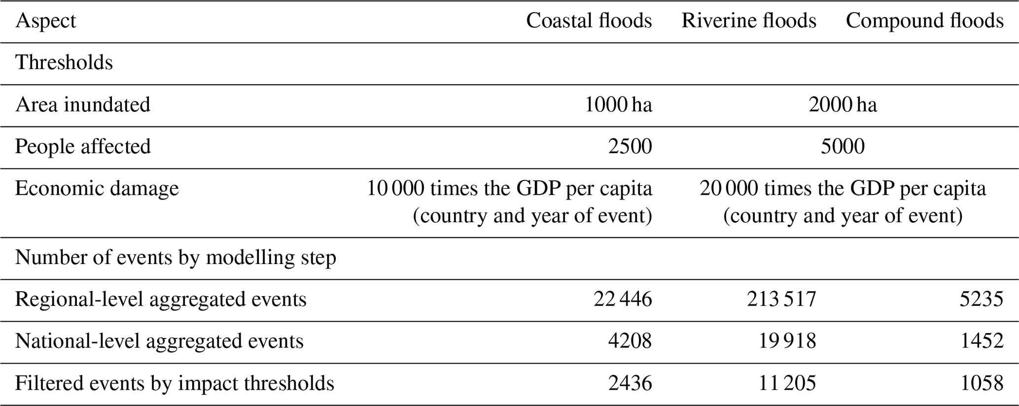
The exact threshold depends on the type of event, and in the case of economic losses, also on the country and year of event, as it was linked to the level of gross domestic product (GDP) per capita (Table 2).
Table 2Thresholds for selecting flood events with the number of filtered events and significant potential impacts.
Thresholds in Table 2 as well as those described earlier in the methodology were selected iteratively based on the following objectives:
-
to maximize the number of modelled events that match observed events from HANZE,
-
to maximize the share of one-to-one relationships between modelled and observed events (as opposed to many-to-one or one-to-many relationships),
-
to minimize the spatial extent of events in terms of affected NUTS3 regions beyond those indicated in HANZE, and
-
to create a list of events that is long enough for statistical analyses and short enough to allow for manual searches through historical records for all events.
To help select the thresholds, observed flood events from the following six datasets were matched per country according to start and end dates:
-
HANZE v2.1 (Paprotny et al., 2023),
-
EM-DAT (Centre for Research on the Epidemiology of Disasters, 2023),
-
European Environment Agency (EEA) flood phenomena (from 1980 only) (European Environment Agency, 2015),
-
Dartmouth Flood Observatory (from 1985 only) (Brakenridge, 2023),
-
Database of Flood Fatalities from the Euro-Mediterranean region (FFEM-DB; from 1980 only) (Papagiannaki et al., 2022), and
-
Recorded Flood Outlines (England only) (Environment Agency, 2023).
In addition, the HANZE dataset was matched with events below the tested thresholds. Following the above objectives results in different potential impact thresholds for coastal and riverine floods. In total, about 43 % of events were filtered out (Table 2).
2.4.3 Comparing modelled and reported events
The modelled flood events of the catalogue were evaluated using gauge records and impact data as well as manual research involving all kinds of documentary sources. At first, English-language papers and local-language flood catalogues providing an overview of the hazard in the country were consulted. National disaster databases were then searched, and the relevant data were extracted. Papers on case studies of disasters were searched for in both English and the local language of the country being researched. A keyword-based search in both English and the local language was performed using a web engine to identify news articles or other online reports mentioning the relevant disasters. In total, 946 major text or data sources were used, 828 of which are listed in the HANZE v2.1 dataset (Paprotny et al., 2023), with the remainder listed together with the data from this study. Based on this information on impacts, each event was categorized into one of the classes listed in Table 3.
Table 3Classification of flood events considering the availability of data sources as well as reported hydrological and socioeconomic impacts. All classes are included in the final flood catalogue.
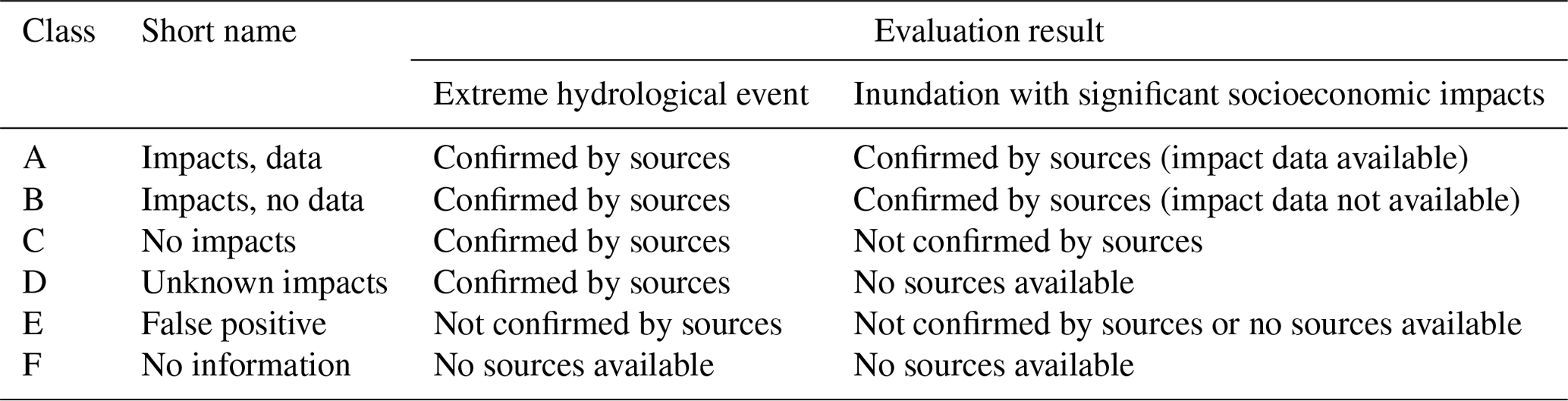
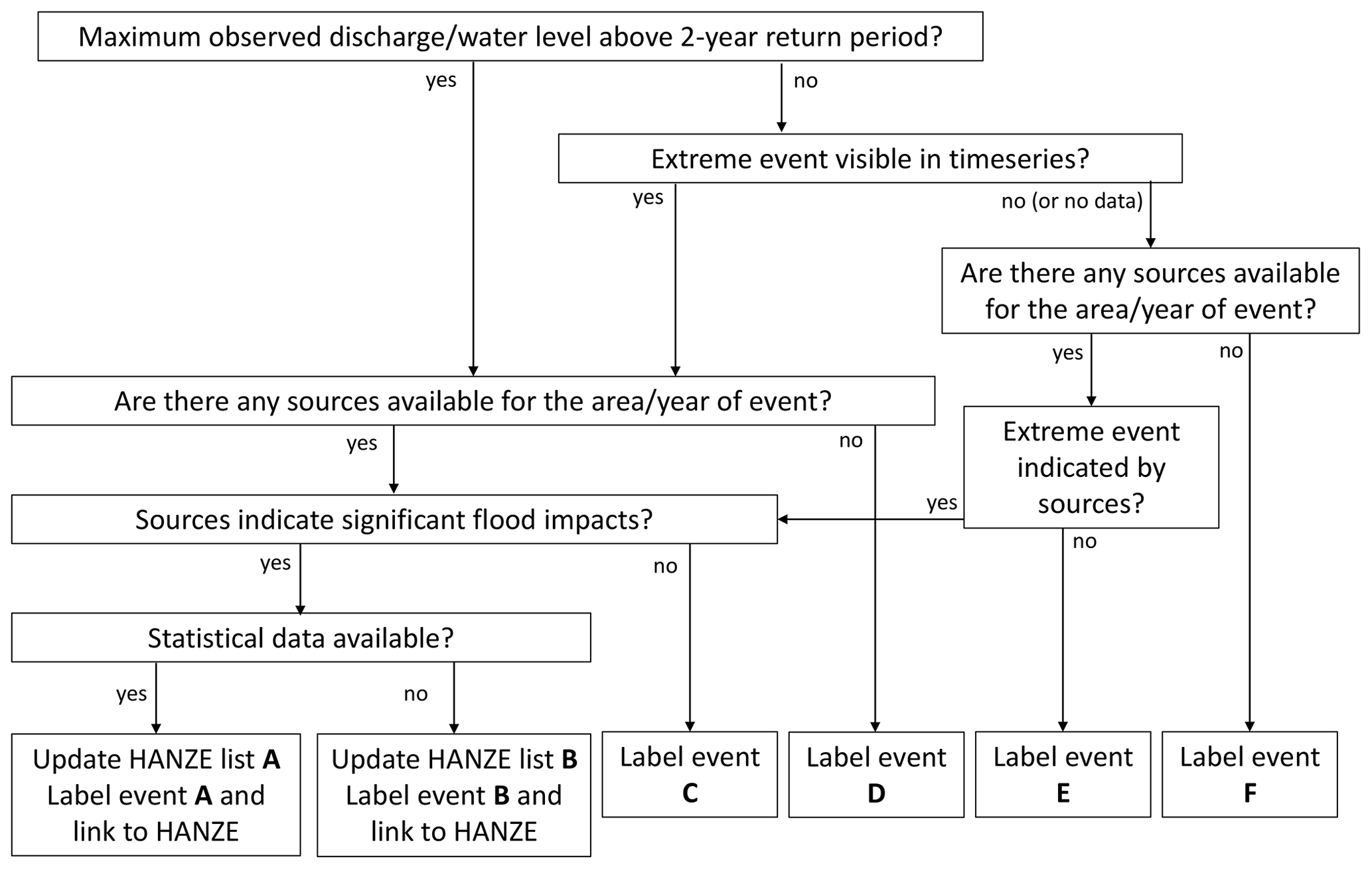
When applying the classification from Table 3, the decision graph from Fig. 2 was used. In general, in the case of complete lack of gauge data or documentary sources, the event was labelled F (“no information”), meaning that no observational data are available and that, therefore, modelled data can be neither confirmed nor rejected. In the case where gauge records were available, the event was first evaluated if the records indicated extreme values. Exceeding a 2-year return period was considered sufficient to confirm that the modelled event was an extreme hydrological event in real life. If the threshold was not exceeded at any of the available gauge stations, the time series was analysed, and the event was considered confirmed to be hydrologically extreme if a flood wave was clearly visible on the dates indicated by the model. If no flood wave was visible, the event was considered a “false positive” (labelled E), i.e. an error in the model that indicates too high a simulated river discharge or sea level. In rare cases, this classification was overridden if documentary sources indicated the occurrence of a flood event. It should be noted that false positives, like all other classes, are maintained in the final flood catalogue so that the users of the data could decide whether to include them in their analyses or not.
For events confirmed to be hydrologically extreme, further analysis concentrated on the occurrence of significant socioeconomic impacts. Significant impacts were defined here in the same way as in the HANZE database (Paprotny et al., 2023) – that is, according to whether they exceed at least one the following thresholds:
-
at least 1000 ha (10 km2) inundated;
-
at least one person killed or missing presumed dead;
-
at least 50 households or 200 people affected, preferably defined as those affected by their homes being inundated by floodwaters or who were evacuated from the inundated area, if the preferred statistic was not available;
-
losses in monetary terms corresponding to at least EUR 1 million in 2020 prices.
In case no further information was available, the event was labelled D (“unknown impacts”). If despite good coverage of sources (e.g. comprehensive local/national flood databases or catalogues), no impacts are mentioned or, in rare cases, direct statement that, for example, a flood emergency did not result in a breach of flood defences, the event was labelled C (“no impacts”). Also, if data on impacts were available, but they did not pass any of the aforementioned thresholds, the event was labelled as no impacts. Events with sufficient information on significant impacts were labelled A (“impacts, data”) and incorporated into the HANZE database. However, if statistical data were not accessible or referred only to a small part of the impacted area, but available descriptions strongly indicated that one of the impact thresholds was likely exceeded, the event was recorded in a separate list of events labelled B (“impacts, no data”). Available historical information was collected for such an event in a database that is a simplified version of HANZE. A detailed description of the data collected in this database, which is made publicly available with this study, is provided in Appendix A1. It should be noted that a match between dates and country with historical events was not enough to label the event A or B. For that, at least one NUTS3 region affected during the event had to be correctly identified by the model.
Additional provisions were made for compound events. If a potential compound flood is indicated in the catalogue but, based on reports and observations, impacts can be attributed only to a coastal flood, the compound event was labelled C (no impacts), the corresponding coastal event A or B and the corresponding riverine event C. The same approach was used if only the riverine driver was responsible for the impacts. Also, if a single-driver event was found to be a false positive (label E), the corresponding compound event was also classified as false positive. In this way, the compound flood definition for events labelled A and B is consistent with the HANZE database, where the interaction of coastal and riverine components is required for a flood to be classified as compound.
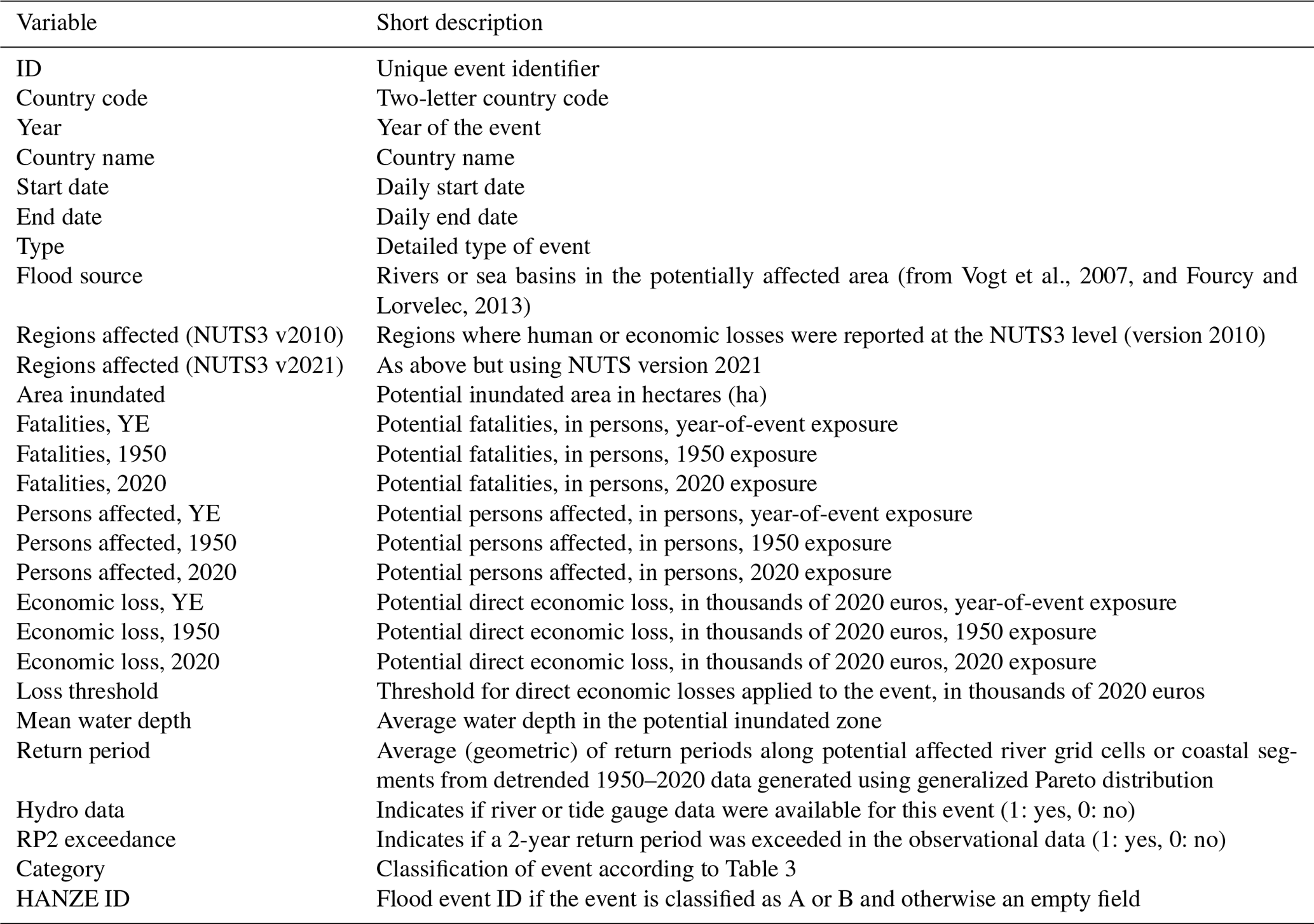
The final flood catalogue consists of two components: (1) a table with all events, indicating their timing, location, potential impacts, hydrological parameters and classification, and (2) the potential flood footprint maps in vector format. The data contained in that table are explained in Appendix A2.
2.5 Validation
The validation of river discharges is presented by Tilloy et al. (2024); however, we used 3442 stations containing daily observations collected for that study for further analysis. The dataset helped us to classify the events in Sect. 2.4.3. Further, we compared extreme discharges observed during riverine and compound events with modelled discharges. Of all station data obtained, 60 % was from the Global Runoff Data Centre and 40 % was from national public datasets of France, Norway, Poland, Spain, Sweden and the United Kingdom. The analysis was limited to 2914 stations with an upstream area of at least 100 km2, which are located in the affected NUTS3 regions according to the model. If the event duration and available gauge series were both at least 30 d, the daily discharge was compared using the Kling–Gupta efficiency, or KGE (Gupta et al., 2009), and Spearman's coefficient of determination (as Pearson's is used in the KGE score). Otherwise, an equal number of days was added before and after the event so that at least 30 observations are used. The maximum daily discharges during the event were also compared.
The validation of the hourly storm surge heights, tide elevations and combined water level was done using 428 tide gauges. Almost all pieces of station data (413) were gathered from the Global Extreme Sea Level Analysis (GESLA) v3 dataset (Haigh et al., 2023), but for better coverage of the eastern Mediterranean Sea, it was complemented by data from seven stations from the POSEIDON system (2024) and, for the southern Baltic Sea, by data from eight stations from the Institute of Meteorology and Water Management – National Research Institute (2023). Apart from validation for all available time series, an event-based validation was done as for river discharges. The default time window for the comparison between modelled and observed data was 7 d unless the event had a longer duration.
Finally, the modelled flood footprints were compared with satellite-derived footprints from the Global Flood Database (GFD; Tellman et al., 2021). The footprints were converted to vector layers, with permanent waterbodies removed from them as per data contained in GFD. Only footprints within NUTS3 regions indicated as affected in the HANZE database were included in the analysis. Population affected within the footprints was derived from HANZE population maps. The flooded area and population affected based on footprints from this study and GFD were compared with reported impacts. Additionally, all flood events in the catalogue with comparative reported impact data were analysed for differences between modelled and reported impacts. Ideally, all modelled impacts should be higher than what was reported, as the intention of the catalogue is to generate potential footprints that do not consider flood protection. Finally, footprints from this study and GFD were compared to derive the hit rate, i.e. the share of the satellite footprints correctly reproduced by the model. This is a similar approach to that used to validate flood hazard maps that are the basis of the modelled footprints (Vousdoukas et al., 2016b; Paprotny et al., 2017; Dottori et al., 2022).
3.1 Flood event catalogue
3.1.1 Modelled impacts by classification
The final catalogue includes 2436 coastal, 11 205 riverine and 1058 compound events with significant potential to have socioeconomic impacts (Fig. 3). This already indicates that a significant proportion of coastal and riverine events might be compound events. The spatial location and time frame of events were matched with at least some gauge observations for 63 % of coastal and 72 % of riverine events. By applying the 2-year return period threshold to observational data, it was possible to immediately confirm that 40 % of coastal and 45 % of riverine events were hydrologically extreme. Further confirmations were obtained through the analysis of gauge time series and documentary records, increasing the confirmation rate to 80 % for coastal, 77 % for riverine and 66 % for compound events. On the other hand, no extreme event was indicated by a gauge or documentary sources for a small part of the catalogue. The false positive ratio (of E events to A–D events) amounts to only 2.2 % (16) for compound, 3.3 % (67) for coastal and 5.2 % (474) for riverine floods.
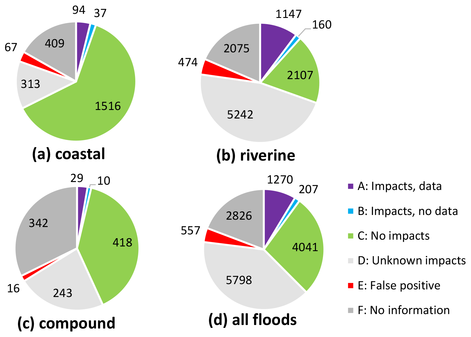
Figure 3Flood events in the catalogue by classification: (a) coastal, (b) riverine and (c) compound. Panel (d) shows totals for all events.
The confirmation of, or at least high confidence in based on available documentary sources, whether the event did or did not result in significant socioeconomic impacts was possible for the majority of coastal and compound events but not for riverine floods. However, the latter occurred by far most frequently, and it was possible to confirm significant socioeconomic impacts for 11.7 % of riverine (1307), 5.4 % of coastal (131) and 3.7 % of compound (39) events (Fig. 3). In some cases, A (impacts, data) events correspond to more than one reported flood in the HANZE database or the events are a combination of A- and B-type (impacts, data and impacts, no data) events. Therefore, the 1270 A and 207 B events actually correspond to 1471 historical floods in HANZE and 237 historical floods without impact data collected in a separate dataset as part of this study (see Appendix A1). This statistic excludes a small number of events that were below the significant impact threshold but indicated a temporal match with the HANZE database. Only 109 such events were identified, of which only two were coastal events and two were compound events. Out of those, only 33 events, all riverine, were spatially matched with HANZE, with a single historical flood in each case. This constitutes only 2 % of matched HANZE events; hence, we can deem the hydrological and socioeconomic thresholds in this study well designed as few HANZE events were missed due to their imposition without creating too many non-impact events. Also, while there were many one-to-many matches between our model and HANZE, largely due to the data-availability rules causing the splitting of some flood events in HANZE, there were only a handful of cases of many-to-one connections.
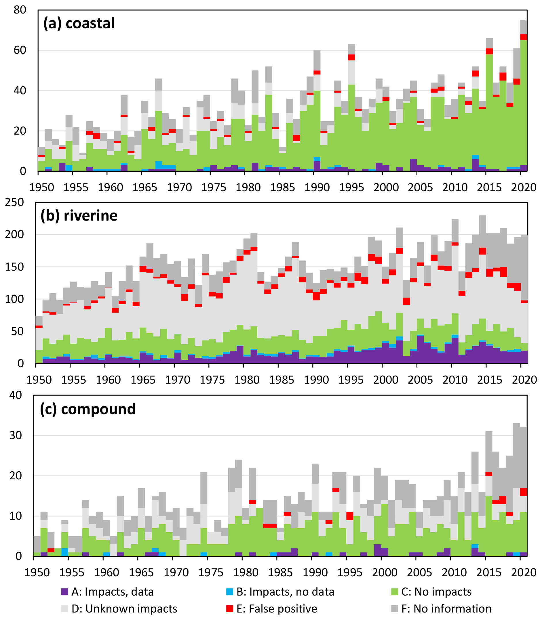
Figure 4Flood events in the catalogue by year and classification: (a) coastal, (b) riverine and (c) compound.
The distribution of events over time (Fig. 4) shows an upward trend, which in the case of A and B events is largely related to better availability of data. There is also better confidence in the non-occurrence of impacts for coastal and compound events in recent decades compared to the beginning of the time series. An increase in F events in the final few years for riverine and compound events is primarily connected with the lower availability of recent river gauge data.
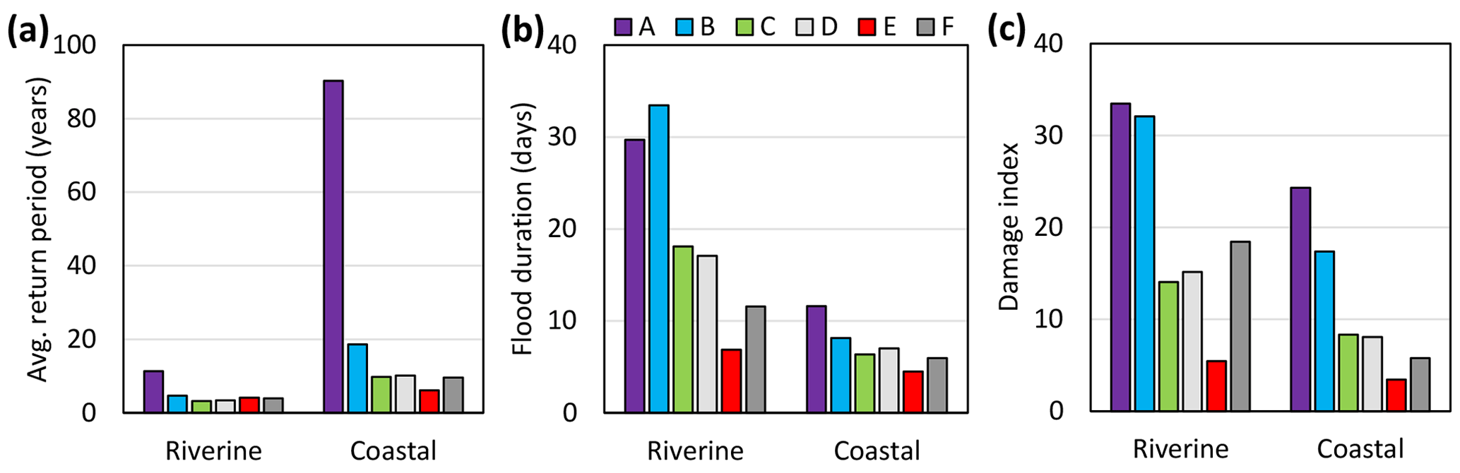
Figure 5Comparison of mean values of selected indicators by main flood type and classification: (a) average return period along affected river or coastal segments, (b) total flood event duration and (c) dimensionless damage index, where 100 equals the highest potential impact of any event in the country during 1950–2020 at constant exposure.
Modelled extremity and impacts of events vary strongly by class (Fig. 5). The return period along affected river and coastal segments is generally much higher for A and B events compared to all others. Indeed, 18 % of coastal and 37 % of riverine events, in which the geometric average of return periods in the affected area was above 25 years, were classified as either A or B. In contrast, when the return period was below 5 years, the values were 2 % and 10 %, respectively. Interestingly, the occurrence of the F class (no information) was only slightly lower for higher return periods. Confirmed impactful events were also longer in duration than other classes, with false positives (E) having the shortest duration. Consequently, the A and B events had, on average, the highest impact potential. In Fig. 5c, the dimensionless damage index is the average of four impact categories (potential area inundated, fatalities, persons affected and economic loss) relative to the maximum impact of any event in the country during 1950–2020 at constant 1950 exposure. False positives had, on average, the lowest impact potential. In all examples, the remaining categories (C: no impacts, D: unknown impacts and F) circled around the average values for all variables analysed in Fig. 5.
3.1.2 Comparison with HANZE reported impacts database
The flood catalogue includes the majority of reported historical floods, with significant socioeconomic impacts since 1950 contained in the HANZE v2.1 database (Paprotny et al., 2023). However, there is a strong difference in the completeness of the catalogue regarding flood type. While about 90 % of coastal, compound and slow-onset riverine floods were modelled, only 55 % of flash floods were captured (Table 4). The latter category, as defined in HANZE, represents short, rapid floods, where the extreme rainfall event triggering the event lasted no more than 24 h, excluding urban floods. As those often occur in small catchments, they are often not captured as the study was limited only to catchments with an upstream area of at least 100 km2.
Table 4Comparison of the number of HANZE events, their footprints and reported impacts with modelled data for 1950–2020. a Only regions classified as compound by the model (regions forming compound events in the HANZE database are not necessarily in the zone directly influenced by both riverine and coastal drivers). b Impact data were not available for all HANZE events.
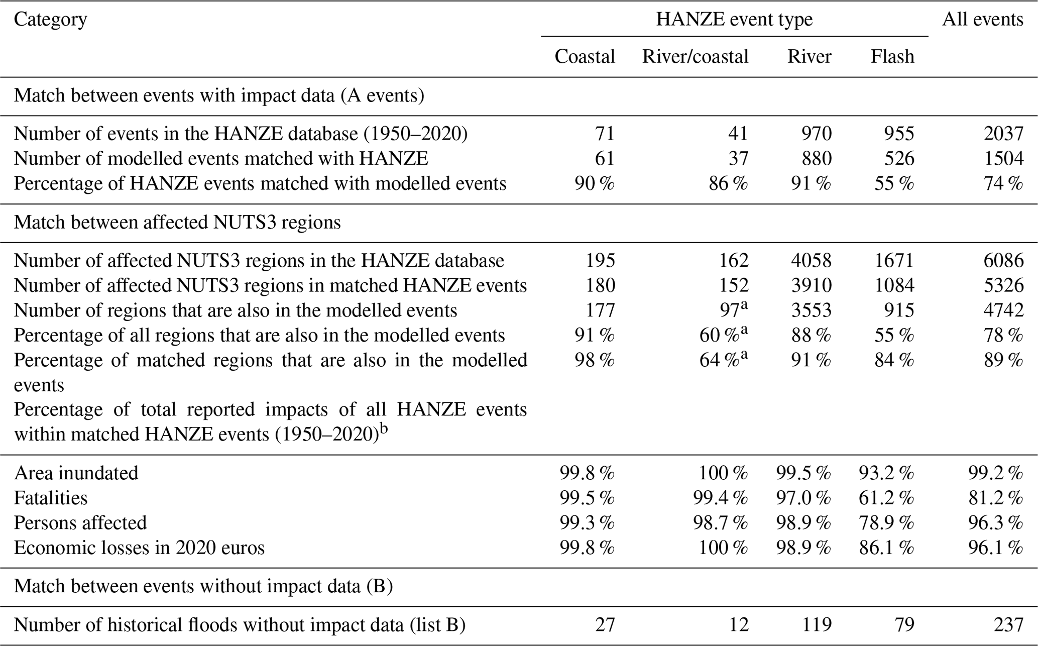
The HANZE database indicates more than 6000 NUTS3-level impacts since 1950. Furthermore, 78 % of those are reproduced by the model (Table 4), which is a slightly higher percentage than the hit rate at event level (74 %). This is largely due to good coverage for slow-onset riverine floods (88 %) compared to flash floods (55 %) when the former affected more regions on average than the latter. For the 1504 events matched by the model, the hit rate of NUTS3 regions for the model is 89 %, which is, again, lower for flash floods (84 %) than for larger riverine events (91 %) and especially coastal floods (98 %). A full list of HANZE events with the information on which of those were captured by the model and which NUTS3 regions were correctly identified is provided together with the dataset in the repository (Paprotny, 2024). In general, the performance of the model is stable over time (Fig. 6), though the share of events correctly identified by the model is lower at the very beginning of the model runs (1950s).
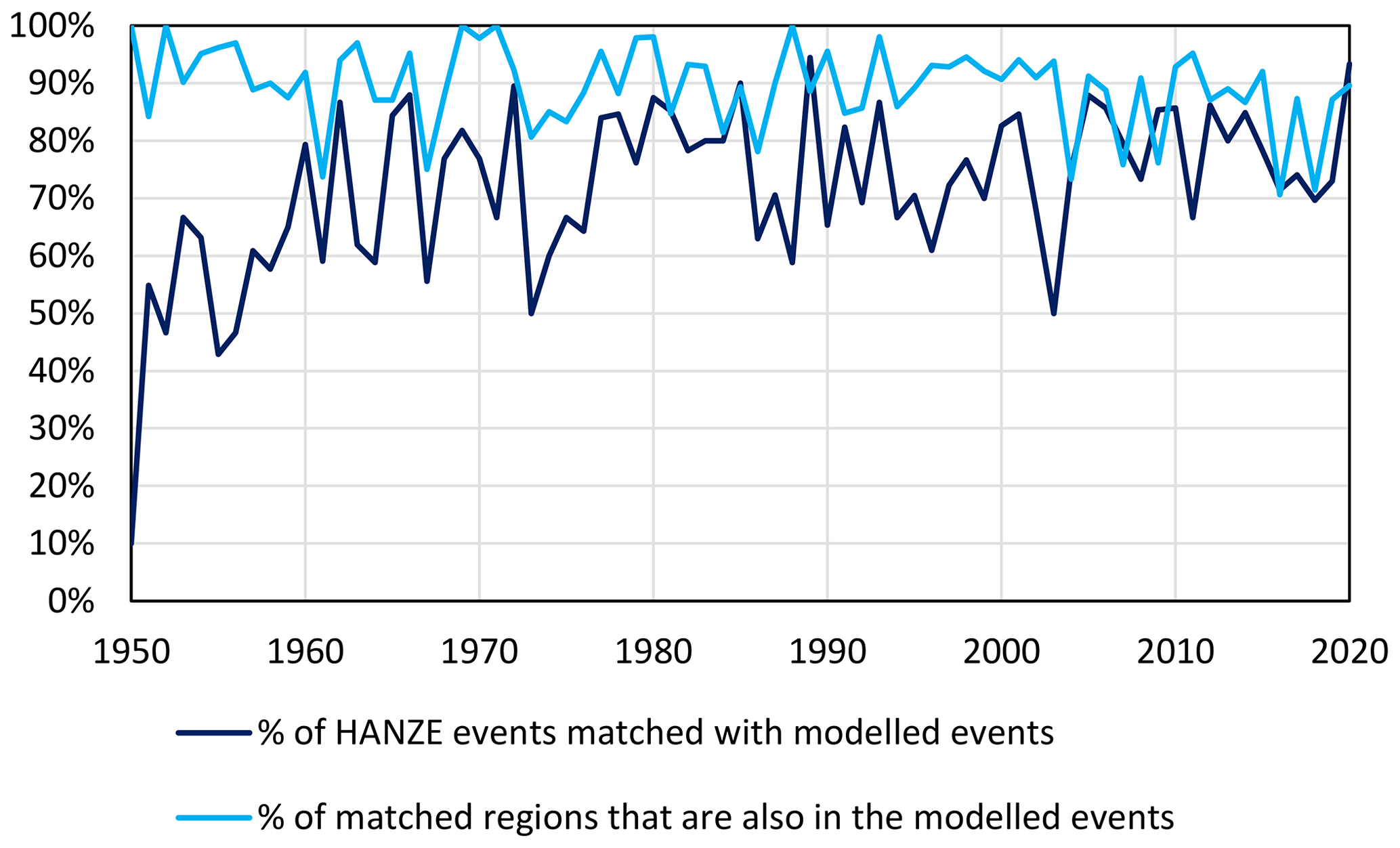
Figure 6Share of HANZE events matched with the model and the share of regions in matched events that is also present in the model.
Analysing the reported impacts in HANZE, even though they are incomplete (except for fatalities), provides further insights. The data in Table 4 show that 97 %–100 % of reported impacts in all four categories for coastal, compound and slow-onset riverine floods were in those historical floods that could also be found in the model. This shows that the model captured almost all large events and that the omissions are mostly minor floods in specific areas where the hazard is apparently not well quantified. For instance, out of 14 omitted coastal and compound floods, 10 are events in Italy occurring mostly before 1964 and affecting 200–500 persons with no more than one fatality (with a single exception of a seven-fatality flood in January 1950). Much lower coverage is again for flash floods as those responsible for 61 % of all fatalities can only be found in the model. For other impact categories, the coverage is better, but historical records are very incomplete in relation to those statistics.
3.2 Modelled potential impacts in the flood catalogue
Without flood protection measures, floods would have large consequences throughout Europe. A simple summation of flood impacts in the catalogue is not informative as it assumes not only no flood protection, but also that population and economic activity move to the frequently affected zone in the first place and then immediately return to previous conditions after each event, even just days after the change. Considering the total number of reported impacts in HANZE v2.1, albeit incomplete, it can be estimated that only about 1 % of potentially inundated area, population and economic assets were actually affected during 1950–2020. The reported flood deaths equal only about 0.01 % of the potential fatalities. Therefore, the potential impacts are merely an intermediate result necessary in the process of estimating flood vulnerability and impact attribution (see Sect. 5). Still, some analysis of the results can be performed as the modelling chain can derive the impact estimates under different exposure scenarios and if we consider it was driven by variable climate conditions.
3.2.1 Temporal changes in potential flood impacts
For all types of events, an increase in the number of potential events and their impacts was recorded (Table 5). Even though the trends are less pronounced under constant exposure scenarios, they are still equivalent to at least 0.3 % of the annual increase in potential coastal flood losses in an average year between 1950 and 2020 in the case of fatalities, 0.5 % in the case of economic loss, and 0.8 % in the case of affected population. For riverine floods, the potential impacts have grown even more, while the strongest increase is indicated for compound floods at a rate of at least 1.9 % yr−1 since 1950. Potential impacts per flood event are rather similar for coastal and riverine events and slightly lower for compound events as the latter category is spatially constrained to regions directly affected by both coastal and riverine drivers.
Table 5Average potential impacts of floods and their trends by flood type and exposure scenario (dynamic year-of-event exposure or fixed at the 1950 or 2020 level). The impacts of compound events mostly overlap with those of coastal and riverine; therefore, they should not be added together. Economic losses are in constant 2020 prices and exchange rates. Note that n/a represents not applicable.
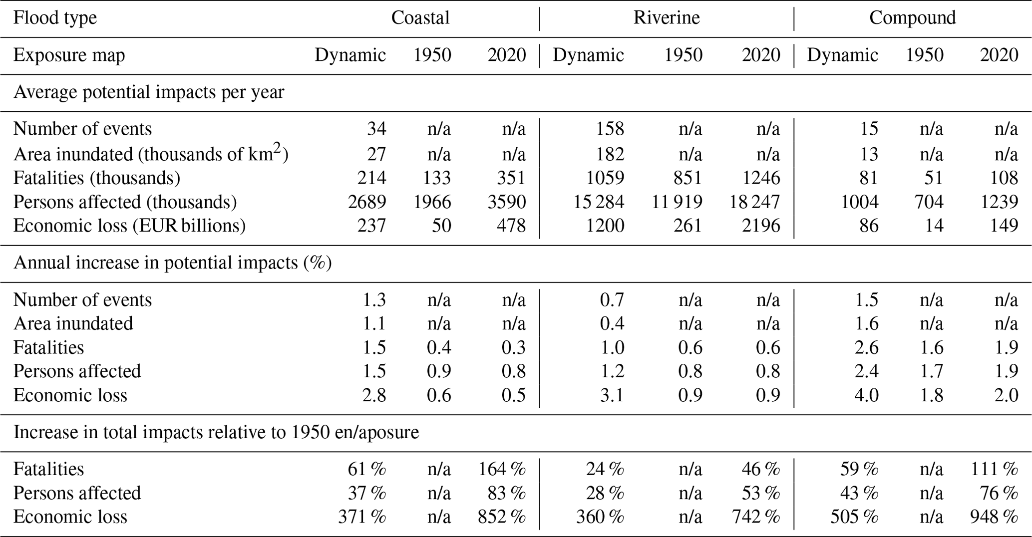
Demographic and economic growth since 1950 has substantially increased potential losses. Presently, the exposure of population to riverine floods is more than 50 % higher than if the population had not increased and nearly twice as high for coastal and compound events. Potential impacts relative to the total population in the study area increase more strongly than in the constant-exposure scenario, indicating stronger population growth in areas prone to coastal and compound flooding relative to areas not at risk. However, only a marginal increase in areas at risk of riverine floods was observed relative to areas not prone to this type of flood.
An enormous increase in gross domestic product (GDP) per capita (2 % yr−1 in the study area) and associated growth in the stock of fixed assets resulted in a 5- to 6-fold increase in potential losses relative to 1950 and an 8- to 10-fold increase in 2020. As the asset growth was higher than GDP, potential economic losses relative to GDP also increased between 1950 and 2020. In contrast to population growth, asset growth in flood-prone areas was only marginally higher or even lower in the case of riverine events than in areas not at risk of flooding.
3.2.2 Spatial distribution of potential flood impacts
Coastal and compound flood potential is highly concentrated in just a few countries (Fig. 7). Though these estimates do not include the effect of flood protection, the top five countries by coastal flood potential are also most prominently featured in the HANZE database in terms of historical coastal flood impacts: the Netherlands, the United Kingdom, Germany, France and Italy. The same group, with the addition of Ireland, also have the most significant compound flood potential. On the other hand, numerous potential coastal and compound floods are present in the catalogue for Greece, but only one historical example for that country could be found in HANZE (a compound flood in 1968 that affected Crete).
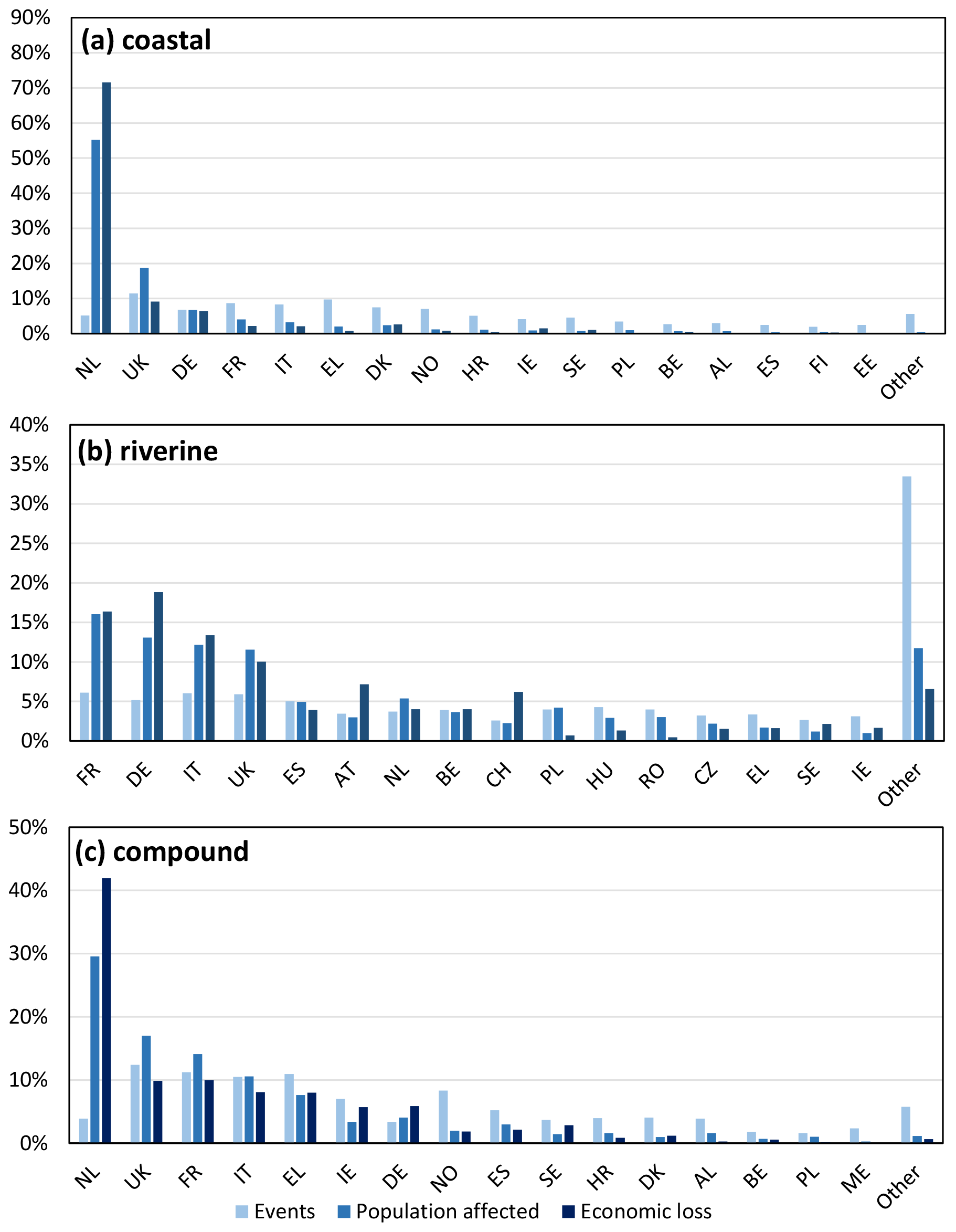
Figure 7Flood events in the catalogue by country and potential impacts given as a percentage of all events: (a) coastal, (b) riverine and (c) compound. Population affected and economic loss is at a constant 2020 exposure level.
In total, the flood catalogue includes coastal floods in 25 countries and compound floods in 24. Slovenia also has no events on the compound flood list as none of the compound events was able to pass the higher socioeconomic thresholds for riverine and compound events. Bosnia and Herzegovina and Montenegro are the only countries on the compound flood list that are not present on the coastal flood list due to the limited risk along their short coastlines. Bulgaria is the only country with access to the sea that is not included in the coastal flood catalogue as no event exceeded the socioeconomic thresholds. One historical case of coastal flooding in Bulgaria (in 1999) was recorded in HANZE.
Riverine flood potential is more evenly distributed in space. All countries highlighted in Fig. 7b have numerous examples of historical damaging floods in HANZE, with the exception of the Netherlands, where historical cases are limited to four floods recorded in the 1990s. In total, 37 out of 42 countries in the study area had at least some potential flood events. Some small countries had no riverine or compound floods in the catalogue as they have no river section with an upstream area bigger than 100 km2.
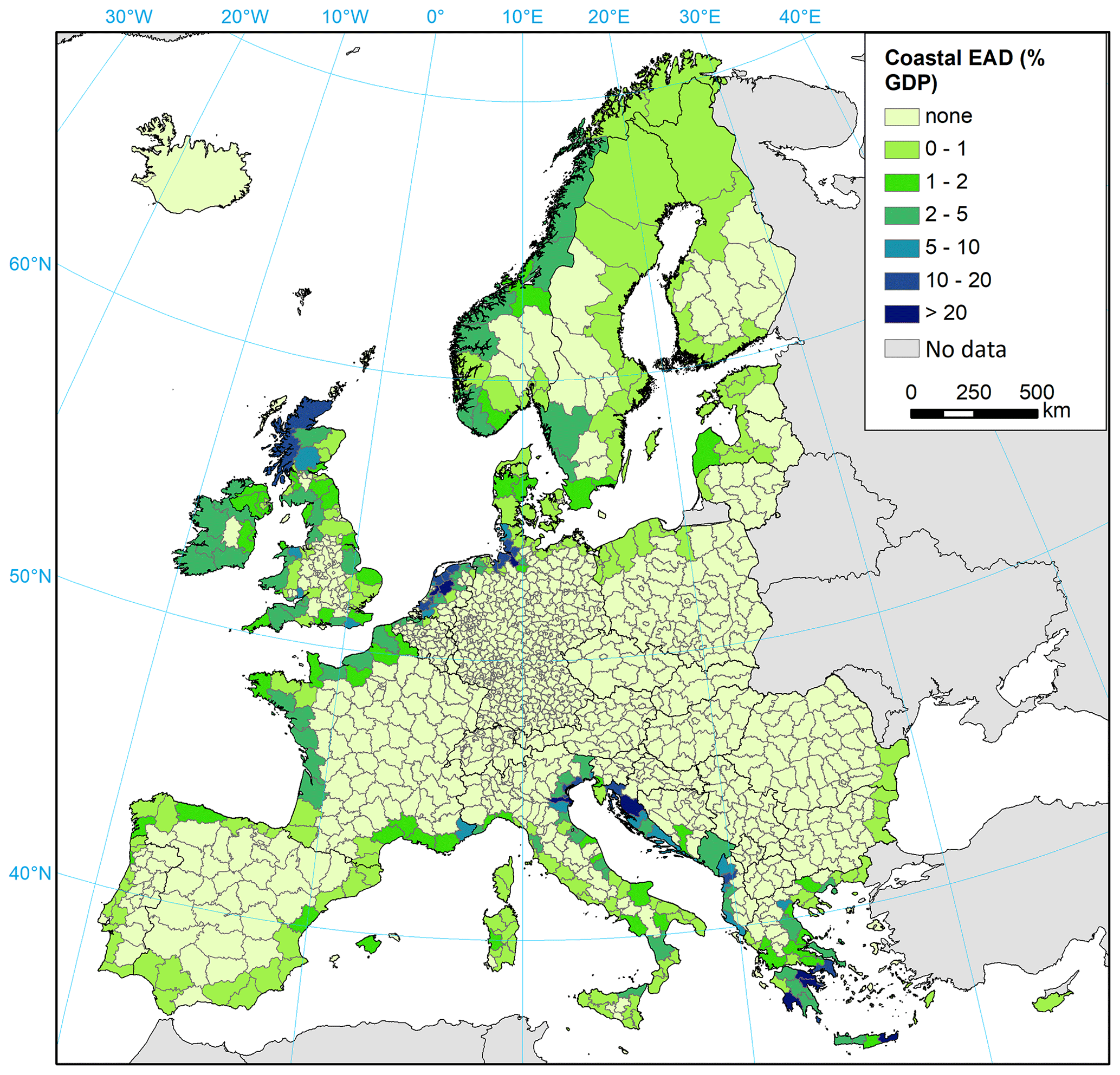
Figure 8Potential expected annual economic damage (EAD) of coastal floods given as a percentage of the GDP for 1950–2020 at a constant 2020 exposure level per NUTS3 region. Potential impacts per region include all events above the 100 ha flooded area threshold per NUTS3 region, including those that do not pass the socioeconomic impact thresholds.
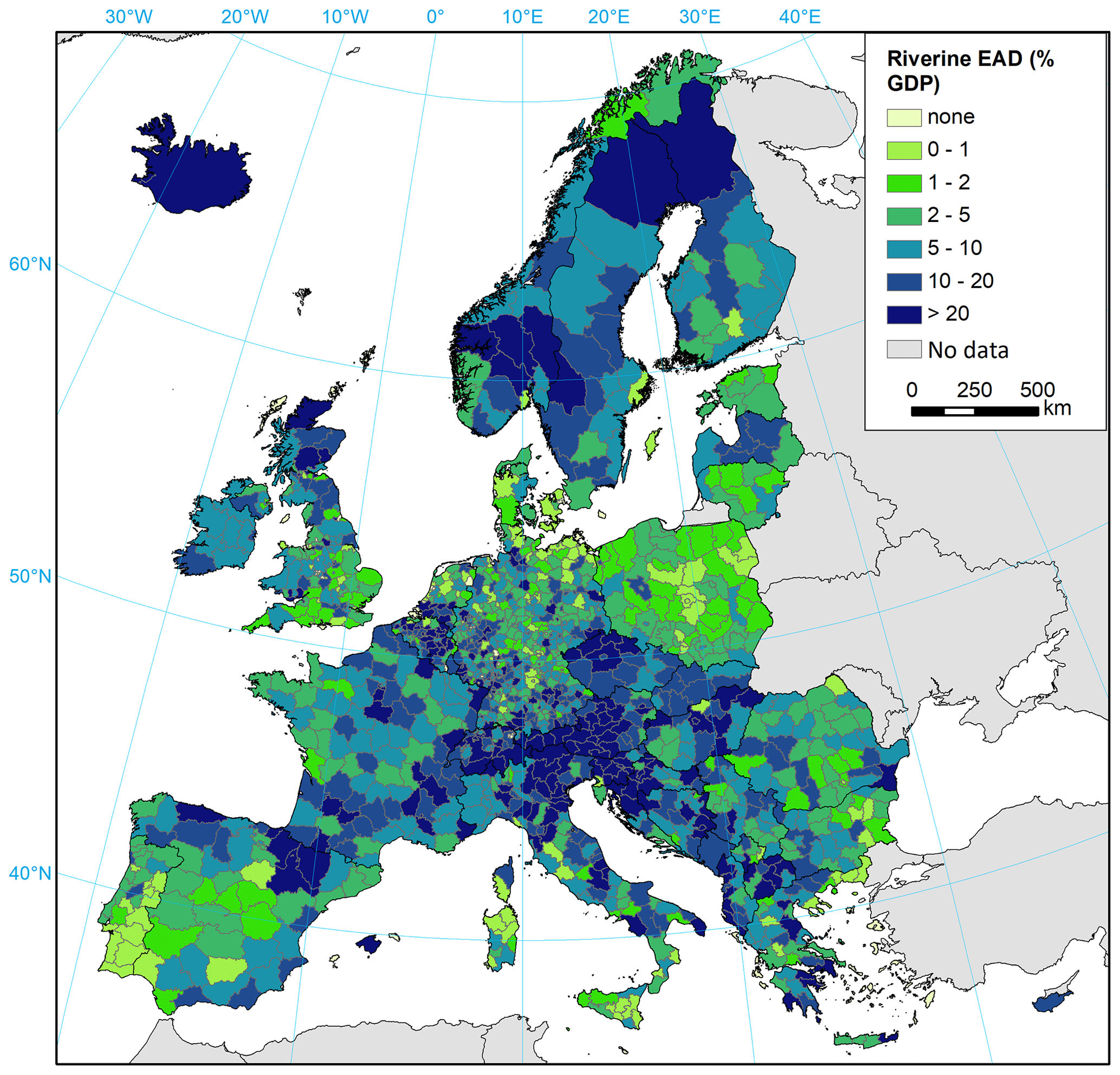
Figure 9Potential expected annual economic damage of riverine floods given as a percentage of the GDP for 1950–2020 at a constant 2020 exposure level per NUTS3 region. Potential impacts per region include all events above the 100 ha flooded area threshold per NUTS3 region, including those that do not pass the socioeconomic impact thresholds.
A variety of indicators can be derived at the level of NUTS3 regions. Here we present one example, potential economic damages normalized to the 2020 exposure level, which is relative to the 2020 gross domestic product (GDP). Along most of the European coast, potential damages resulting from storm surges are limited (Fig. 8), with the risk concentrated along the North Sea, Adriatic Sea and Aegean Sea. Locations of the most significant past coastal floods stand out (the Netherlands, German Bight and Venice). Riverine damage potential is much higher (Fig. 9) and concentrated around main European mountain ranges (Alps, Carpathians, Pyrenees and Dinaric Alps) as well as Scandinavia and the British Isles. Risk is noticeably lower along the North European Plain, southwestern Iberian Peninsula and southern Great Britain. However, it must be stressed that the data represent only damage potential without considering flood protection or other forms of adaptation.
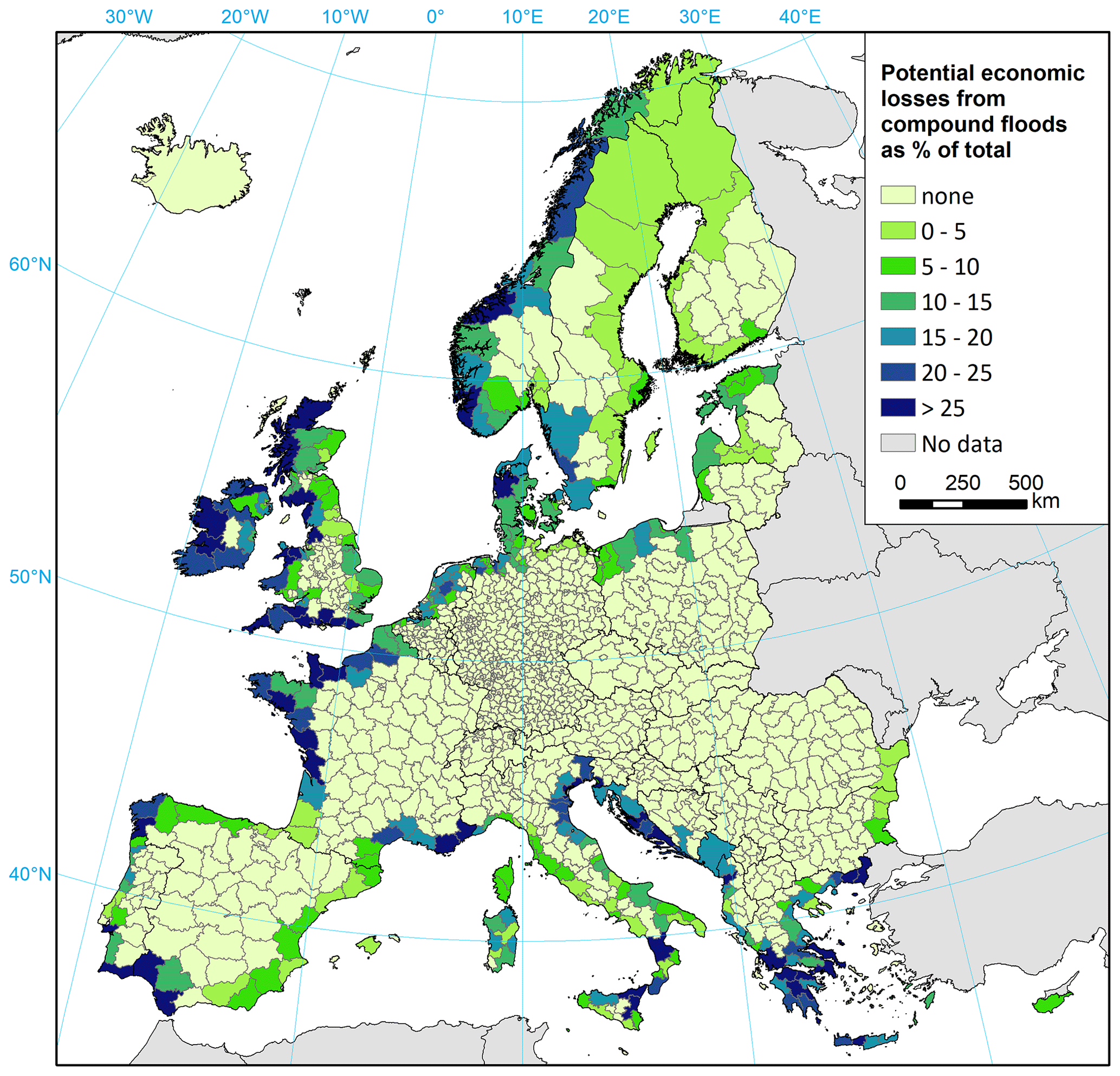
Figure 10Share of compound floods is total potential economic losses for 1950–2020 at a constant 2020 exposure level per NUTS3 region. Potential impacts per region include all events above the 100 ha flooded area threshold per NUTS3 region, including those that do not pass the socioeconomic impact thresholds. Individual riverine and coastal events that contribute to compound events were excluded to compute this metric.
In some parts of Europe, the possibility of the co-occurrence of coastal and riverine floods could have large implications on risk. Figure 10 maps the share of compound flood potential at the regional level relative to the total. For each NUTS3 region, we derived a list of all flood events with a potential inundated area of 100 ha in size – that is, before aggregation and application of socioeconomic thresholds – and then removed the riverine and coastal events that overlapped with compound events. This way, it was possible to avoid double counting and to sum together the remaining flood events. The results (Fig. 10) show that compound potential is very unevenly distributed across Europe. In northern and eastern coasts of the Adriatic Sea; Greece; Ireland; western and southern coasts of Great Britain; and certain parts of France, Italy, Spain and Norway, compound events could potentially contribute 20 %–25 % or even more of all economic losses from flooding. In all aforementioned countries, there are known examples of damaging floods that are contained in the HANZE database.
3.3 Validation
3.3.1 Extreme river discharges
At least one river discharge station with adequate data length was available for 7742 events (63 % of the total), and nearly 292 000 time series were identified within the NUTS3 regions potentially affected by those events. Most of the data are available for events that occurred in the United Kingdom, Poland, Spain, Sweden, Germany, France, and Norway. The R2 between modelled and observed peak discharge for all event time series, standardized according to the reported upstream area, is 0.45. However, the relative discharges are of more interest of this study, and modelled peak discharges corrected for difference in average annual discharges have an R2 of 0.63. The time series of the daily discharge during the events is good (0.5–0.75) or very good (0.75–1) for 59 % of all station–event combinations in terms of Spearman's R2 and for 30 % in terms of the KGE score. On the other hand, poor (0–0.2) or very poor (< 0) performance was recorded for 18 % and 41 % of stations, respectively. There is relatively little difference in performance depending on the classification of events, except for far worse results for events classified as false positives (E). Here, a poor or very poor score was recorded for 83 % of station–event combinations, compared to 37 % for HANZE flood events (A). Performance also varies strongly by location (Fig. 11), with, for example, Germany, Ireland, Austria, Belgium and Slovakia recording much higher shares of good or very good station performance (above 40 %) than, for example, Poland, Spain, Sweden and Portugal (less than 25 %).
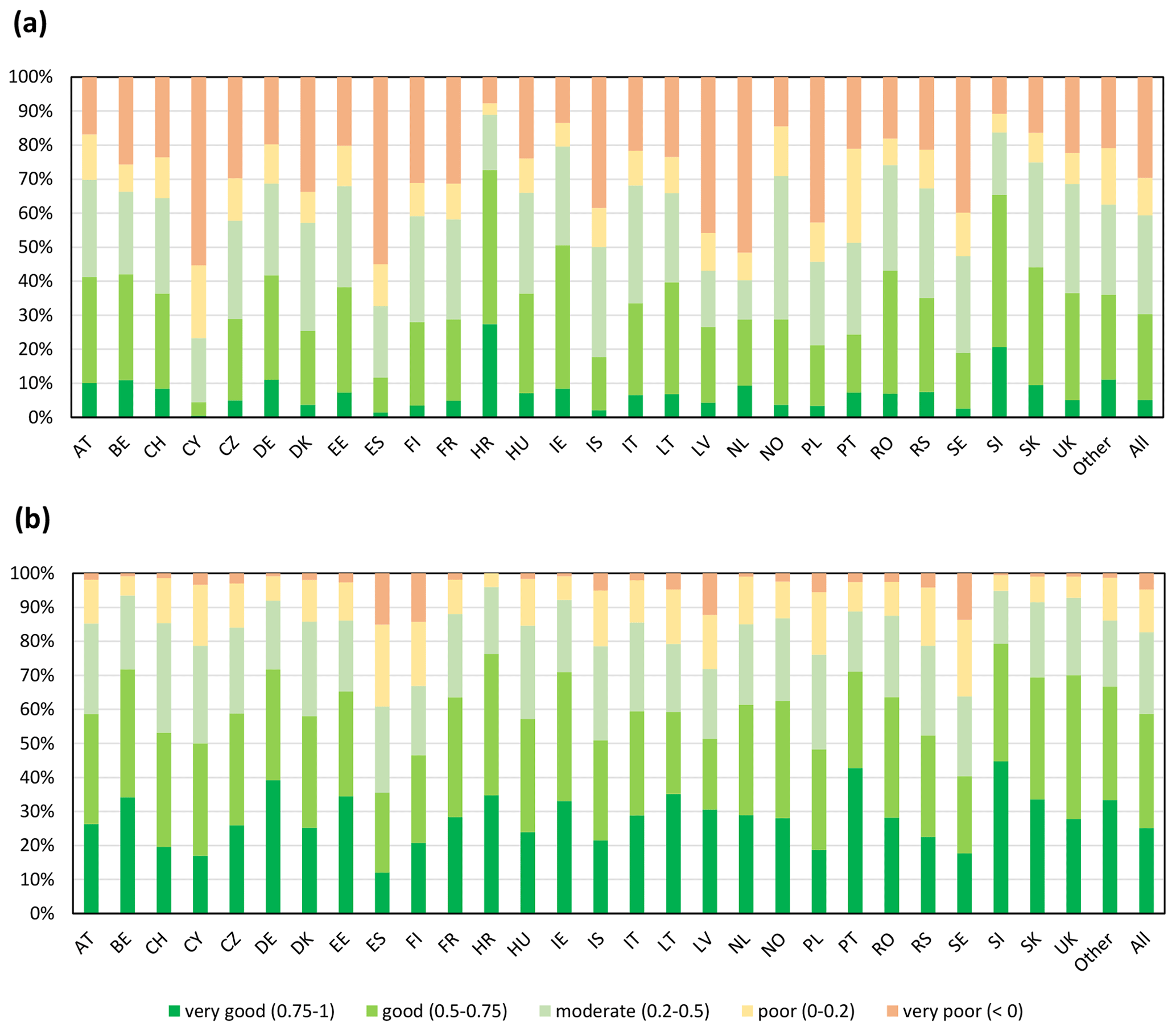
Figure 11Comparison of daily river discharge during flood events in the catalogue for a 30 d window centred around the dates of the event. Abbreviations are NUTS level 0 country codes. The graph shows the percentage of all stations per country by performance class: (a) KGE score and (b) Spearman's coefficient of determination.
3.3.2 Extreme sea levels
At least one tide gauge with an adequate data length was available for 1363 events (56 % of the total), and a total of 8102 time series were identified within the NUTS3 regions potentially affected by those events. Most of the data are available for events that occurred in the United Kingdom, Denmark, Norway, the Netherlands, France, Sweden and Germany. The overall results are compared using several metrics in Table 6. Overall, the maximum sea levels observed during the various potential coastal floods were well reproduced, with the main source of inaccuracies being storm surge heights. Further, 80 % of modelled time series spanning the duration of the events indicated a good or very good R2 when compared with observations. For tides and total water level, such performance was measured for 93 %–94 % of stations. The best performance of the storm surge model was recorded for North and Baltic seas (Fig. 12), with far lower performance for the eastern Mediterranean Sea. However, potential flood events and observational data are both relatively scarce in the latter region, which also had the lowest scores for reproducing tides and combined sea level. As in the case of riverine events, there is little variation between events by classification, though historical HANZE events (A) had slightly higher scores for the combined sea level and storm surge heights than all other classes. This could be, to some extent, the result of the difference in the geographical distribution of events.
Table 6Comparison between maximum hourly sea level and its components during flood events in the catalogue for a 7 d window centred around the dates of the event.
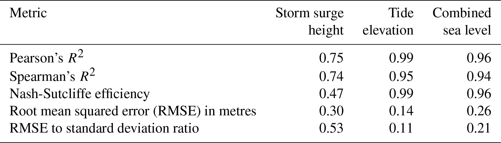
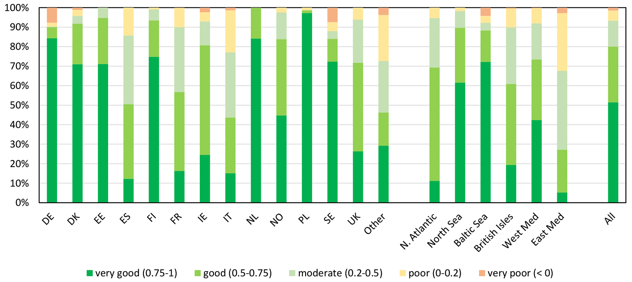
Figure 12Comparison between maximum hourly storm surge height during flood events in the catalogue for a 7 d window centred around the dates of the event. The graph shows the percentage of all stations per country that have different values of Pearson's R2. Abbreviations on the left side of the graph are NUTS level 0 country codes. On the right side of the graph, stations are grouped by main European sea regions (N. Atlantic: exposed north Atlantic Ocean coasts – mostly France and Spain; North Sea: includes Norwegian coasts; Baltic Sea: includes Danish straits; British Isles: coasts of Great Britain and Ireland; West Med and East Med: western and eastern Mediterranean Sea, respectively).
3.3.3 Comparison of flood footprints
The comparison of modelled potential flood impacts with impacts based on satellite-derived flood footprints and actual impacts recorded in the HANZE database highlights the challenge of correctly recreating past floods (Table 7). For exactly half of the 20 floods for which a satellite-derived footprint is available, our modelled population affected was closer to reported population affected than estimates based on satellite-derived flood footprints and vice versa. In most cases, satellite-derived footprints severely underestimated the extent of the flooding, with the exception of floods in the United Kingdom, where they indicated many times higher affected population numbers than the actual impact reported. In all cases, the modelled area and persons affected were higher than the actual impact, as was the intention of the catalogue, modelled without flood protection. However, there is a very close match in persons affected during the August 2002 flood in Czechia and Germany. In the whole catalogue, the area affected was higher than reported in 83 % of cases where the actual impact was reported in HANZE (i.e. 256 out of 307), fatalities were higher in 98 % of cases (1473 out of 1496), population affected was higher in 89 % of cases (686 out of 773) and economic loss was higher in 89 % of cases (675 out of 755).
Table 7Comparison of modelled potential flood zone with satellite-derived footprints from the Global Flood Database (Tellman et al., 2021) and reported impacts from HANZE (Paprotny et al., 2023) for several European floods for 2002–2015. The area flooded is given in square kilometres. ∗ Percentage of the satellite flood footprint reproduced by the modelled flood footprint of this study.
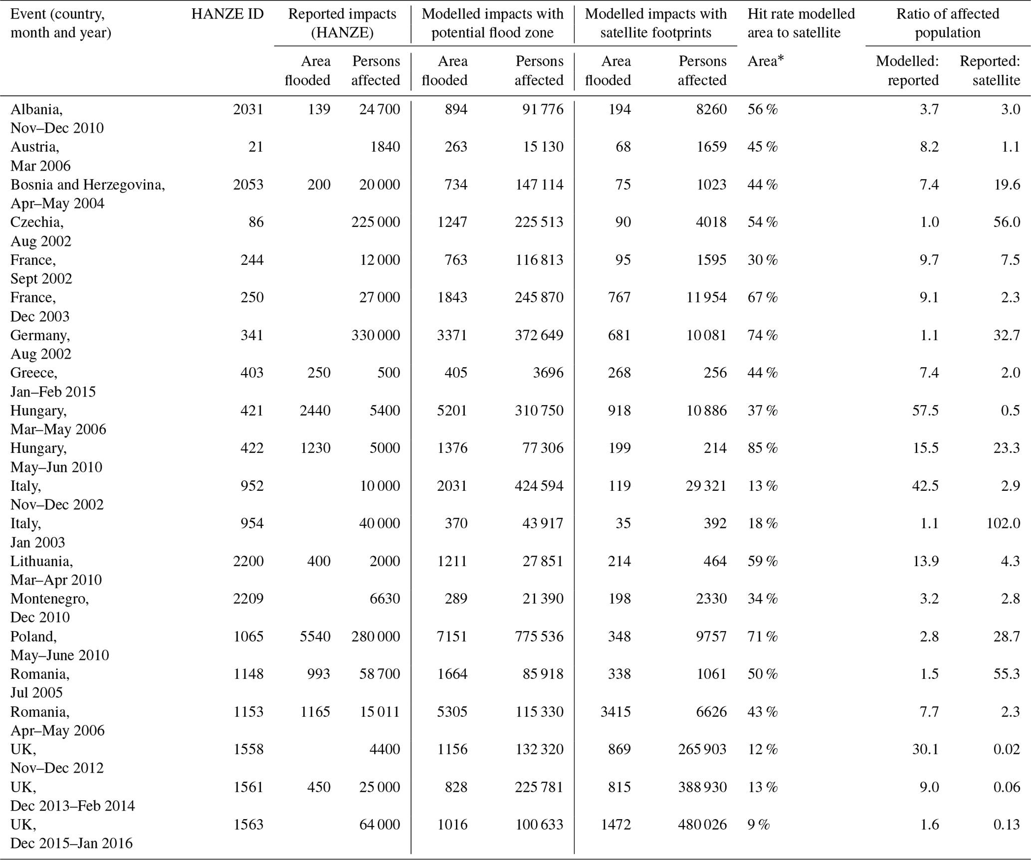
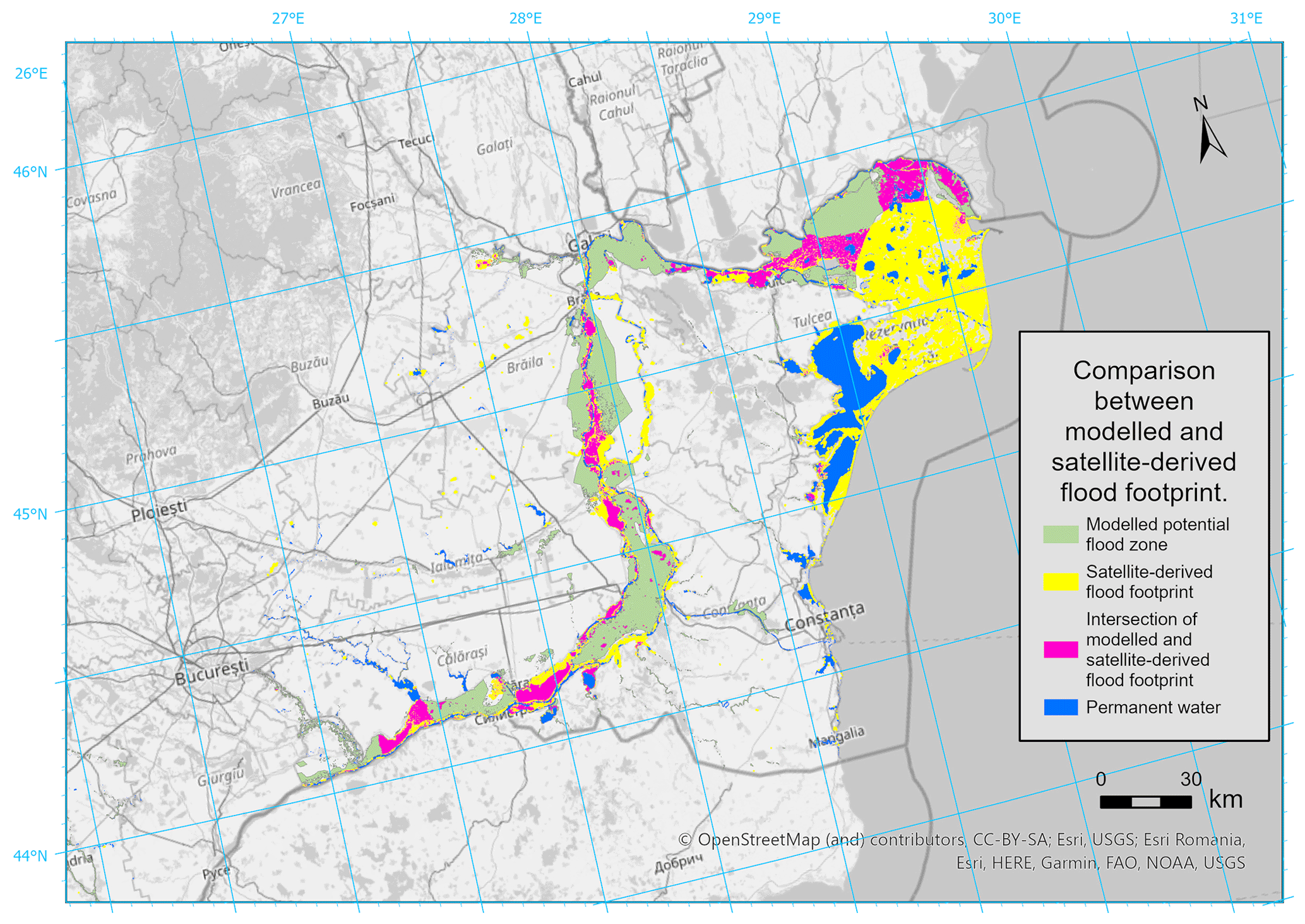
Figure 13Example comparison between modelled and satellite-derived flood footprint of the 2006 event in Romania. © OpenStreetMap contributors 2024. Distributed under the Open Data Commons Open Database License (ODbL) v1.0.
A direct comparison between modelled and satellite footprints (Fig. 13) has shown that the hit rate, i.e. the share of the satellite footprints correctly reproduced by the model, varied between 30 % and 85 %, except for events in Italy and the United Kingdom, where it was only 9 %–18 %. However, the satellite footprints also performed very poorly against reported losses for those floods. Some additional flood events were analysed but were not included in Table 7 as the satellite footprints showed virtually no population affected, which is in high contrast to actual impacts. Such a situation occurred, for example, for the summer floods in the United Kingdom in 2007 that flooded homes of about 192 000 people (HANZE database number 1546), almost none of which could be reproduced with satellite flood footprints.
4.1 Uncertainties and limitations of the models and modelled data
The elaborate modelling chain that involves both riverine and coastal processes is subject to multiple cascading limitations and uncertainties. The starting point of the simulations are input climate data derived from global reanalyses. Though ERA5 and ERA5-Land are state-of-the-art reanalysis products, they still encounter problems of inhomogeneities, gaps or errors in observational data, model biases, and limitations in representing precipitation extremes in particular (Hersbach et al., 2020; Muñoz-Sabater et al., 2021). In the case of the riverine model, bias-adjustment and downscaling were carried out, but it is also only statistical transformation that depends on the quality of high-resolution observations as well (see Sect. 4.2).
Validation results in Sect. 3.1 indicate mostly good performance of the models in reconstructing past extreme discharges and sea levels but not in all areas. Some regions are more challenging to model than others – for example, due to a complex topography or shoreline or strong anthropogenic influence on the water cycle (especially through reservoirs). Not all types of floods or processes that drive them could be represented. Most noticeably, the resolution of the riverine model is inadequate for capturing smaller flash floods as the hydrological model has a spatial resolution of 1′ driven by climate data that were downscaled twice (first from ERA5 to ERA5-Land and then using the ISIMIP3BASD method) and a temporal resolution of 6 h. Additionally, flood hazard maps used to generate the footprints only covered catchments with an upstream area of at least 100 km2. Consequently, 91 % of slow-onset riverine floods, but only 55 % of flash floods, from HANZE were reproduced. Urban floods are not represented at all (also in the HANZE dataset).
Further, no flood defences are represented in the model, which is this way by design, as information on this aspect is scarce, especially in the temporal dimension. At the same time, a flood that was historically prevented by existing defences might not have been prevented under counterfactual conditions. We also hypothesize that flood protection levels are driven to some extent by flood risk and flood occurrence (Sect. 4.2). The use of flood hazard maps for a defined set of scenarios enables the generation of flood footprints without carrying out a computationally infeasible continuous hydrodynamic simulation over a period of 71 years. However, the maps assume a specific hydrograph which is not necessarily valid for all floods with the same peak discharge. Further, the three sets of maps (including two sets for different catchment sizes) are methodologically different and were created for diverse sets of scenarios. Although the coastal maps were rerun specifically for this study based on the results of the extreme sea level modelling, the riverine maps are from previous studies. Their application is problematic in some locations due to inconsistencies in river network delineation between the European Flood Awareness System (EFAS) and the hazard maps. The accuracy of the riverine flood hazard maps is also variable depending on the region and the probability of occurrence (see Paprotny et al., 2017, and Dottori et al., 2022, for details).
Compound floods are represented by merging riverine and coastal flood zones, which neglects the possible interaction between the storm surge and river discharge that could generate higher water levels than is possible for individual drivers. Additionally, not all coastal processes are included in the model, such as interaction between tide and storm surges or influence of SLR on tide elevations. Wave run-up is only approximated by taking one-fifth of offshore significant wave height as more precise estimates would require a very detailed model of the nearshore. Finally, long-term land motion is limited to GIA due to a lack of detailed data on the subject.
4.2 Uncertainties and limitations of the observations and documentary sources
The results are influenced by not only the accuracy of models, but also that of the observations. Our river discharge simulations are driven by reanalysis data that were downscaled and bias-adjusted using interpolated meteorological observations, the accuracy of which strongly depends on the density of point meteorological data. As shown in Thiemig et al. (2022), precipitation during extreme events in the EMO dataset can at times significantly diverge from other reported measurements. Though our meteorological input data are still driven primarily by ERA5, the reanalysis itself is influenced by the availability of meteorological data, which is very inhomogeneous in time (Hersbach et al., 2020). This might be the reason for the noticeably lower performance of our model in reproducing flood events in the 1950s.
Model calibration and validation as well as classification of the flood event catalogue are affected by the availability of tide and river gauges (Sect. 3.1.1 and 3.1.2). The data are unevenly distributed, with most data available for northern Europe, in particular the Nordic countries and the British Isles. On the other hand, very limited data were available for Italy, Greece and Balkan countries. It is further uneven in time, with both the 1950s and the last few years until 2020 having lower coverage than the 1990s and 2000s in particular. Identification of events as false positives (E) is also potentially problematic as in large NUTS3 regions the only available observations could be outside the impact zone of the event, hence incorrectly suggesting that the model generated a “bogus” event. Satellite-derived footprints were used to compare the modelled flood footprints but themselves often widely diverged from reported impacts. The hit rate between satellite and model data varied significantly between individual events, similar to what was observed in a reconstruction of recent European coastal floods by Le Gal et al. (2023).
Similarly, documentary sources on socioeconomic impacts of floods are highly uneven in quality between countries. For instance, while there are comprehensive databases and flood catalogues accessible, for example, for France, Italy, Norway, Portugal, Spain, Switzerland or even some Balkan countries, the scattering of information makes it very laborious to collect data for other countries – for example, Austria, Germany and the United Kingdom. Many compilations of flood impacts only cover the recent 2 decades, while older flood catalogues published in the 1980s or 1990s often have no newer follow-ups. This strongly affects the frequency of C (no impacts) events relative to D (impacts unknown). Thanks to extensive research contained in the HANZE database, this has less of an effect on the detection of A (impacts, data) and B (impacts, no data) events. Still, uncertainty surrounds the designation of flood events as having “significant” socioeconomic impacts. The thresholds defined in HANZE are somewhat arbitrary, though they are based on the experience of collecting more than 2500 records in the dataset. In the case of smaller events, their classification is uncertain if the data are incomplete or not very accurate. This is potentially problematic for B events, where, at times, no quantitative data at all are available, and the classification was based only on the description of impacts. Finally, NUTS3 regions, the principal socioeconomic unit of observation here and in HANZE, vary in size in terms of both area and population. It might be slightly easier for floods in large regions to exceed a regional-scale threshold for a minimum flood area in the model and to be considered affected in HANZE, where regional-scale impact thresholds are also applied when detailed damage data are available.
This study is the largest attempt to reconstruct past flood losses in Europe and makes an advance toward the full decomposition of drivers of historical flood losses. We created a flood catalogue for Europe that contain 14 699 events with significant socioeconomic impact potential. It covers riverine, coastal and compound events over a period of 71 years and considers the evolving human impact on catchments, climate change and growing exposure. However, it should be highlighted that the damage estimates provided in the catalogue exclude the influence of flood defences and spatial and temporal variation in vulnerability levels.
The catalogue includes 1504 out of 2037 damaging floods since 1950 that are included in HANZE dataset (Paprotny et al., 2023), including about 90 % of coastal, compound and slow-onset riverine floods and 55 % of flash floods. The coverage of reported impacts of those events is 81 %–99 % depending on the exact measure. The performance of the model is relatively stable over time, though it is slightly worse for the 1950s.
The flood catalogue was primarily devised as the baseline (factual) reconstruction of past floods in Europe. However, it can also be directly used for multiple applications. The immediate follow-up to this analysis will be modelling changes in flood preparedness in Europe during the past 70 years, including flood protection standards and relative losses (Paprotny et al., 2024). The modelling chain can be further used with counterfactual climate inputs. Methods such as ATTRIbuting Climate Impacts (ATTRICI; Mengel et al., 2021) enable the removal of the global warming effect from all variables required to model riverine discharges. Additional counterfactual simulations are possible to quantify the human influence on catchments, in particular through the construction of reservoirs (Boulange et al., 2021). Methods such as transformed-stationary extreme value analysis (Mentaschi et al., 2016) can be used to detrend storm surge heights as well as remove the long-term sea level rise. Together with HANZE historical exposure maps (Paprotny and Mengel, 2023), counterfactual scenarios for all components of risk would be achieved. This would provide the first comprehensive impact attribution of European flood losses and generate an important reference dataset for pan-European flood risk assessments.
A1 Contents of list B of historical floods
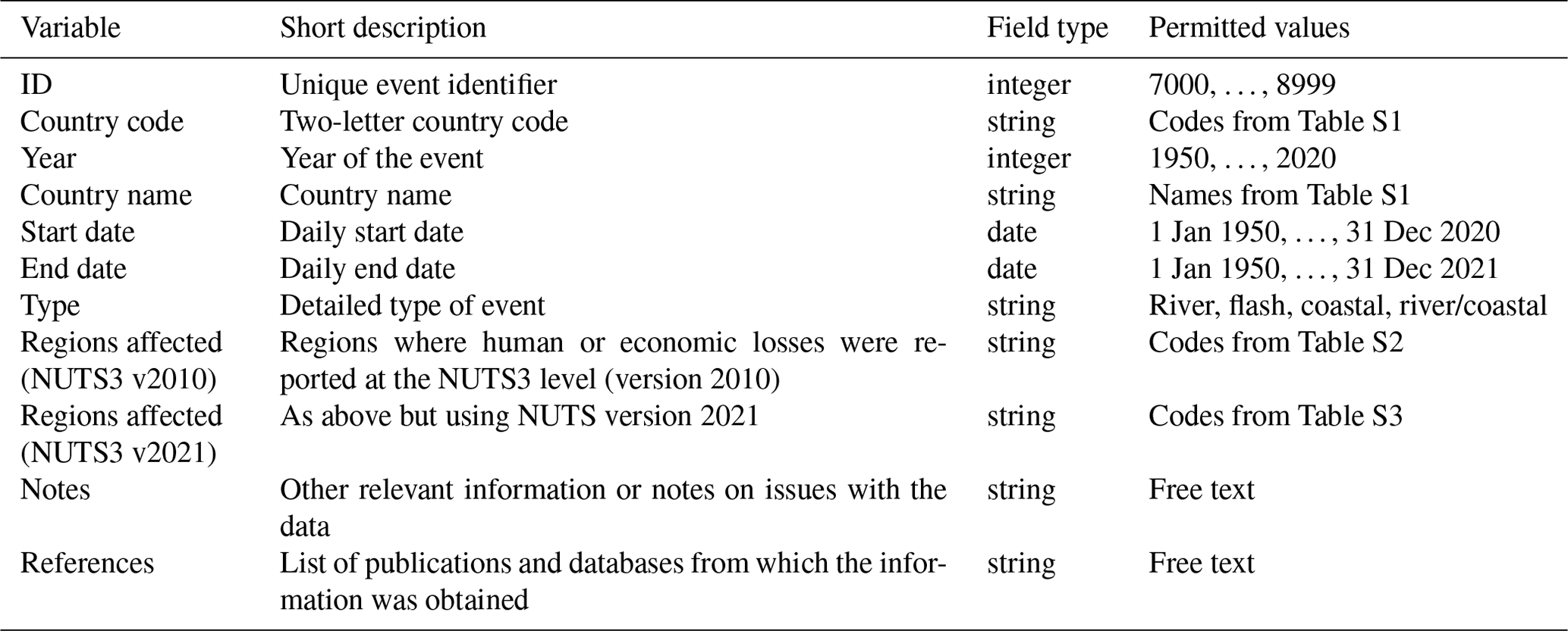
The format of the database of events in list B follows the format of the HANZE database (Paprotny et al., 2023), with a reduced number of fields as events were confined to list B specifically due to a lack of relevant data (primarily flood impact statistics). Most fields have strictly defined permitted values, except “Notes”, which includes an explanation of why impacts should be considered significant (using partial available data or descriptive indicators), and “Data sources”, which lists all cited references. The latter is often the same as used in the HANZE database; therefore, only publications specific to list B are included in the full bibliographic details provided with the event file. For detailed discussion about the contents of each field, we refer the reader to Paprotny et al. (2023).
Table A1Summary of fields recorded in list B of floods. Tables S1–S3 are available on Zenodo at https://doi.org/10.5281/zenodo.11259233 (Paprotny, 2024c).
A2 Contents of the modelled flood event catalogue
Table A2Summary of fields recorded in the modelled flood event catalogue.
A3 Availability of data and models
Table A3Availability of input and output data and models from the study. Models are indicated in italics.
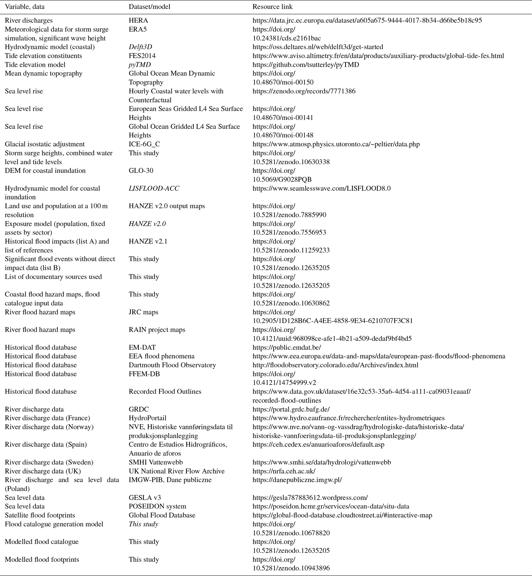
All links were accessed on 20 August 2024.
The main code for generating the flood catalogue is available on Zenodo (https://doi.org/10.5281/zenodo.10678820, Paprotny, 2024b). More links to other models and code are provided in Appendix A3.
Numerous public datasets and models were used in the study, the results of which are also publicly available. Details on where to find each dataset and model are provided in Appendix A3. The flood event catalogue is publicly available for download (https://doi.org/10.5281/zenodo.12635205, Paprotny, 2024a) with additional data (https://doi.org/10.5281/zenodo.10630338, Paprotny, 2024d; https://doi.org/10.5281/zenodo.10630862, Paprotny, 2024e; https://doi.org/10.5281/zenodo.10943896, Paprotny, 2024f), and also can be viewed, filtered, and analysed on the HANZE website (https://naturalhazards.eu/, NaturalHazards, 2024).
DP developed the concept, implemented the methods, collected and processed most of the data, and acquired funding. BR collected part of the historical impact data and performed part of the flood event classification. MIV computed coastal flood hazard maps. PT and JS performed the comparison based on satellite-derived flood footprints and created the online visualization of the study. FD and ST contributed datasets and methods for the riverine and coastal simulations, respectively. LF and HK helped to develop the concept and methods. All authors wrote the paper.
The contact author has declared that none of the authors has any competing interests.
Publisher's note: Copernicus Publications remains neutral with regard to jurisdictional claims made in the text, published maps, institutional affiliations, or any other geographical representation in this paper. While Copernicus Publications makes every effort to include appropriate place names, the final responsibility lies with the authors.
This article is part of the special issue “Methodological innovations for the analysis and management of compound risk and multi-risk, including climate-related and geophysical hazards (NHESS/ESD/ESSD/GC/HESS inter-journal SI)”. It is not associated with a conference.
We would like to thank the referees, Oliver Wing and Helena Garcia, for their useful comments.
This research has been supported by the German Research Foundation (DFG) through project “Decomposition of flood losses by environmental and economic drivers” (FloodDrivers) (grant no. 449175973).
The article processing charges for this open-access publication were covered by the Potsdam Institute for Climate Impact Research (PIK).
This paper was edited by Anais Couasnon and reviewed by Oliver Wing and Helena Garcia.
Andreadis, K. M., Wing, O. E., Colven, E., Gleason, C. J., Bates, P. D., and Brown, C. M.: Urbanizing the floodplain: Global changes of imperviousness in flood-prone areas, Environ. Res. Lett., 17, 104024, https://doi.org/10.1088/1748-9326/ac9197, 2022.
Argus, D. F., Peltier, W. R., Drummond, R., and Moore, A. W.: The Antarctica component of postglacial rebound model ICE-6G_C (VM5a) based upon GPS positioning, exposure age dating of ice thicknesses, and relative sea level histories, Geophys. J. Int., 198, 537–563, https://doi.org/10.1093/gji/ggu140, 2014.
Arnal, L., Asp, S.-S., Baugh, C., de Roo, A., Disperati, J., Dottori, F., Garcia, R., Garcia Padilla, M., Gelati, E., Gomes, G., Kalas, M., Krzeminski, B., Latini, M., Lorini, V., Mazzetti, C.,Mikulickova, M., Muraro, D., Prudhomme, C., Rauthe-Schöch, A., Rehfeldt, K., Salamon, P., Schweim, C., Skoien, J. O., Smith, P., Sprokkereef, E., Thiemig, V., Wetterhall, F., and Ziese, M.: EFAS upgrade for the extended model domain – technical documentation, Publications Office of the European Union, Luxembourg, https://doi.org/10.2760/806324, 2019.
Bates, P. D., Horritt, M. S., and Fewtrell, T. J.: A simple inertial formulation of the shallow water equations for efficient two-dimensional flood inundation modelling, J. Hydrol., 387, 33–45, https://doi.org/10.1016/j.jhydrol.2010.03.027, 2010.
Bednar-Friedl, B., Biesbroek, R., Schmidt, D. N., Alexander, P., Børsheim, K. Y., Carnicer, J., Georgopoulou, E., Haasnoot, M., Le Cozannet, G., Lionello, P., Lipka, O., Möllmann, C., Muccione, V., Mustonen, T., Piepenburg, D., and Whitmarsh, L.: Europe, Climate Change 2022: Impacts, Adaptation and Vulnerability, Contribution of Working Group II to the Sixth Assessment Report of the Intergovernmental Panel on Climate Change, Cambridge University Press, Cambridge, UK and New York, NY, USA, 1817–1927, https://doi.org/10.1017/9781009325844.015, 2022.
Blöschl, G., Kiss, A., Viglione, A., Barriendos, M., Böhm, O., Brázdil, R., Coeur, D., Demarée, G., Llasat, M. C., Macdonald, N., Retsö, D., Roald, L., Schmocker-Fackel, P., Amorim, I., Belinová, M., Benito, G., Bertolin, C., Camuffo, D., Cornel, D., Doctor, R., Elleder, L., Enzi, S., Garcia, J. C., Glaser, R., Hall, J., Haslinger, K., Hofstätter, M., Komma, J., Limanówka, D., Lun, D., Panin, A., Parajka, J., Petric, H., Rodrigo, F. S., Rohr, C., Schönbein, J., Schulte, L., Silva, L. P., Toonen, W., Valent, P., Waser, J., and Wetter, O.: Current flood-rich period is exceptional compared to the past 500 years in Europe, Nature, 583, 560–566, https://doi.org/10.1038/s41586-020-2478-3, 2020.
Boulange, J., Hanasaki, N., Yamazaki, D., and Pokhrel, Y.: Role of dams in reducing global flood exposure under climate change, Nat. Commun., 12, 417, https://doi.org/10.1038/s41467-020-20704-0, 2021.
Boyd, E., Levitan, M., and van Heerden, I.: Improvements in Flood Fatality Estimation Techniques Based on Flood Depths, in: Wind Storm and Storm Surge Mitigation, edited by: Uddin, N., American Society of Civil Engineers, Reston, Virginia, USA, 126–139, https://doi.org/10.1061/9780784410813.ch11, 2010.
Brakenridge, G. R.: Global Active Archive of Large Flood Events. Dartmouth Flood Observatory, University of Colorado, http://floodobservatory.colorado.edu/Archives/index.html (last access: 26 October 2023), 2023.
Burek, P., van der Knijff, J., and De Roo, A.: LISFLOOD – Distributed Water Balance and Flood Simulation Model - Revised User Manual 2013, Publications Office of the European Union, Luxembourg, https://doi.org/10.2788/24982, 2013.
Centre for Research on the Epidemiology of Disasters: EM-DAT, CRED/UCLouvain, Brussels, Belgium, https://www.emdat.be/ (last access: 26 October 2023), 2023.
Choulga, M., Moschini, F., Mazzetti, C., Grimaldi, S., Disperati, J., Beck, H., Salamon, P., and Prudhomme, C.: Technical note: Surface fields for global environmental modelling, EGUsphere [preprint], https://doi.org/10.5194/egusphere-2023-1306, 2023.
Copernicus Emergency Management Service: European Flood Awareness System (EFAS) version 5.0, https://confluence.ecmwf.int/display/CEMS/European+Flood+Awareness+System (last access: 8 November 2023), 2023.
Diederen, D., Liu, Y., Gouldby, B., Diermanse, F., and Vorogushyn, S.: Stochastic generation of spatially coherent river discharge peaks for continental event-based flood risk assessment, Nat. Hazards Earth Syst. Sci., 19, 1041–1053, https://doi.org/10.5194/nhess-19-1041-2019, 2019.
Dottori, F., Alfieri, L., Bianchi, A., Skoien, J., and Salamon, P.: A new dataset of river flood hazard maps for Europe and the Mediterranean Basin, Earth Syst. Sci. Data, 14, 1549–1569, https://doi.org/10.5194/essd-14-1549-2022, 2022.
Gupta, H. V., Kling, H., Yilmaz, K. K., and Martinez, G. F.: Decomposition of the mean squared error and NSE performance criteria: Implications for improving hydrological modelling, J. Hydrol., 377, 80–91, https://doi.org/10.1016/j.jhydrol.2009.08.003, 2009.
Enríquez, A. R., Wahl, T., Marcos, M., and Haigh, I. D.: Spatial footprints of storm surges along the global coastlines, J. Geophys. Res.-Oceans, 125, e2020JC016367, https://doi.org/10.1029/2020JC016367, 2020.
Environment Agency: Recorded Flood Outlines, data.gov.uk, https://www.data.gov.uk/dataset/16e32c53-35a6-4d54-a111-ca09031eaaaf/recorded-flood-outlines (last access: 31 October 2023), 2023.
European Environment Agency: Flood phenomena, EEA, https://www.eea.europa.eu/data-and-maps/data/european-past-floods/flood-phenomena (last access: 26 October 2023), 2015.
European Space Agency and Sinergise: Copernicus Global Digital Elevation Model, OpenTopography [data set], https://doi.org/10.5069/G9028PQB, 2021.
Eurostat: Statistical regions in the European Union and partner countries NUTS and statistical regions 2021 – re-edition 2022, Publications Office of the European Union, Luxembourg, https://doi.org/10.2785/321792, 2022.
Fourcy, D. and Lorvelec, O.: A new digital map of limits of oceans and seas consistent with high-resolution global shorelines, J. Coastal Res., 29, 471–477, https://doi.org/10.2112/JCOASTRES-D-12-00079.1, 2013.
Frieler, K., Volkholz, J., Lange, S., Schewe, J., Mengel, M., del Rocío Rivas López, M., Otto, C., Reyer, C. P. O., Karger, D. N., Malle, J. T., Treu, S., Menz, C., Blanchard, J. L., Harrison, C. S., Petrik, C. M., Eddy, T. D., Ortega-Cisneros, K., Novaglio, C., Rousseau, Y., Watson, R. A., Stock, C., Liu, X., Heneghan, R., Tittensor, D., Maury, O., Büchner, M., Vogt, T., Wang, T., Sun, F., Sauer, I. J., Koch, J., Vanderkelen, I., Jägermeyr, J., Müller, C., Rabin, S., Klar, J., Vega del Valle, I. D., Lasslop, G., Chadburn, S., Burke, E., Gallego-Sala, A., Smith, N., Chang, J., Hantson, S., Burton, C., Gädeke, A., Li, F., Gosling, S. N., Müller Schmied, H., Hattermann, F., Wang, J., Yao, F., Hickler, T., Marcé, R., Pierson, D., Thiery, W., Mercado-Bettín, D., Ladwig, R., Ayala-Zamora, A. I., Forrest, M., and Bechtold, M.: Scenario setup and forcing data for impact model evaluation and impact attribution within the third round of the Inter-Sectoral Impact Model Intercomparison Project (ISIMIP3a), Geosci. Model Dev., 17, 1–51, https://doi.org/10.5194/gmd-17-1-2024, 2024.
Ganguli, P., Paprotny, D., Hasan, M., Güntner, A., and Merz, B.: Projected changes in compound flood hazard from riverine and coastal floods in Northwestern Europe, Earths Future, 8, e2020EF001752, https://doi.org/10.1029/2020EF001752, 2020.
Haigh, I. D., Marcos, M., Talke, S. A., Woodworth, P. L., Hunter, J. R., and Hague, B. S.: GESLA Version 3: A major update to the global higher-frequency sea-level dataset, Geosci. Data J., 10, 293–314, https://doi.org/10.1002/gdj3.174, 2023.
Hersbach, H., Bell, B., Berrisford, P., Hirahara, S., Horányi, A., Muñoz-Sabater, J., Nicolas, J., Peubey, C., Radu, R., Schepers, D., Simmons, A., Soci, C., Abdalla, S., Abellan, X., Balsamo, G., Bechtold, P., Biavati, G., Bidlot, J., Bonavita, M., De Chiara, G., Dahlgren, P., Dee, D., Diamantakis, M., Dragani, R., Flemming, J., Forbes, R., Fuentes, M., Geer, A., Haimberger, L., Healy, S., Hogan, R. J., Hólm, E., Janisková, M., Keeley, S., Laloyaux, P., Lopez, P., Lupu, C., Radnoti, G., de Rosnay, P., Rozum, I., Vamborg, F., Villaume, S., and Thépaut, J.-N.: The ERA5 global reanalysis, Q. J. Roy. Meteor. Soc., 146, 1999–2049, https://doi.org/10.1002/qj.3803, 2020.
Huizinga, J., de Moel, H., and Szewczyk, W.: Global flood depth-damage functions. Methodology and the database with guidelines, Publications Office of the European Union, Luxembourg, https://doi.org/10.2760/16510, 2017.
Institute of Meteorology and Water Management – National Research Institute: Dane publiczne, IMGW-PIB, https://danepubliczne.imgw.pl/ (last access: 11 November 2023), 2023.
Jacob, D., Petersen, J., Eggert, B., Alias, A., Christensen, O. B., Bouwer, L. M., Braun, A., Colette, A., Déqué, M., Georgievski, G., Georgopoulou, E., Gobiet, A., Menut, L., Nikulin, G., Haensler, A., Hempelmann, N., Jones, C., Keuler, K., Kovats, S., Kröner, N., Kotlarski, S., Kriegsmann, A., Martin, E., van Meijgaard, E., Moseley, C., Pfeifer, S., Preuschmann, S., Radermacher, C., Radtke, K., Rechid, D., Rounsevell, M., Samuelsson, P., Somot, S., Soussana, J.-F., Teichmann, C., Valentini, R., Vautard, R., Weber, B., and Yiou, P.: EURO-CORDEX: new high-resolution climate change projections for European impact research, Reg. Environ. Change, 14, 563–578, https://doi.org/10.1007/s10113-013-0499-2, 2014.
Jones, P. W.: First- and Second-Order Conservative Remapping Schemes for Grids in Spherical Coordinates, Mon. Weather Rev., 127, 2204–2210, https://doi.org/10.1175/1520-0493(1999)127<2204:FASOCR>2.0.CO;2, 1999.
Jonkman, S. N., Vrijling, J. K., and Vrouwenvelder, A. C. W. M.: Methods for the estimation of loss of life due to floods: a literature review and a proposal for a new method, Nat. Hazards, 46, 353–389, https://doi.org/10.1007/s11069-008-9227-5, 2008.
Klein Goldewijk, K., Beusen, A., Doelman, J., and Stehfest, E.: Anthropogenic land use estimates for the Holocene – HYDE 3.2, Earth Syst. Sci. Data, 9, 927–953, https://doi.org/10.5194/essd-9-927-2017, 2017.
Kreibich, H., Blauhut, V., Aerts, J. C. J. H., Bouwer, L. M., Van Lanen, H. A. J., Mejia, A., Mens, M., and Van Loon, A. F.: How to improve attribution of changes in drought and flood impacts, Hydrolog. Sci. J., 64, 1–18, https://doi.org/10.1080/02626667.2018.1558367, 2019.
Kreibich, H., Van Loon, A. F., Schröter, K., Ward, P. J., Mazzoleni, M., Sairam, N., Abeshu, G. W., Agafonova, S., AghaKouchak, A., Aksoy, H., Alvarez-Garreton, C., Aznar, B., Balkhi, L., Barendrecht, M. H., Biancamaria, S., Bos-Burgering, L., Bradley, C., Budiyono, Y., Buytaert, W., Capewell, L., Carlson, H., Cavus, Y., Couasnon, A., Coxon, G., Daliakopoulos, I., de Ruiter, M. C., Delus, C., Erfurt, M., Esposito, G., François, D., Frappart, F., Freer, J., Frolova, N., Gain, A. K., Grillakis, M., Grima, J. O., Guzmán, D. A., Huning, L. S., Ionita, M., Kharlamov, M., Khoi, D. N., Kieboom, N., Kireeva, M., Koutroulis, A., Lavado-Casimiro, W., Li, H., Llasat, M. C., Macdonald, D., Mård, J., Mathew-Richards, H., McKenzie, A., Mejia, A., Mendiondo, E. M., Mens, M., Mobini, S., Mohor, G. S., Nagavciuc, V., Ngo-Duc, T., Nguyen, H. T. T., Nhi, P. T. T., Petrucci, O., Quan, N. H., Quintana-Seguí, P., Razavi, S., Ridolfi, E., Riegel, J., Sadik, M. S., Savelli, E., Sazonov, A., Sharma, S., Sörensen, J., Souza, F. A. A., Stahl, K., Steinhausen, M., Stoelzle, M., Szalińska, W., Tang, Q., Tian, F., Tokarczyk, T., Tovar, C., Tran, T. V. T., Van Huijgevoort, M. H. J., van Vliet, M. T. H., Vorogushyn, S., Wagener, T., Wang, Y., Wendt, D. E., Wickham, E., Yang, L., Zambrano-Bigiarini, M., Blöschl, G., and Di Baldassarre, G.: The challenge of unprecedented floods and droughts in risk management, Nature, 608, 80–86, https://doi.org/10.1038/s41586-022-04917-5, 2022.
Kreibich, H., Schröter, K., Di Baldassarre, G., Van Loon, A. F., Mazzoleni, M., Abeshu, G. W., Agafonova, S., AghaKouchak, A., Aksoy, H., Alvarez-Garreton, C., Aznar, B., Balkhi, L., Barendrecht, M. H., Biancamaria, S., Bos-Burgering, L., Bradley, C., Budiyono, Y., Buytaert, W., Capewell, L., Carlson, H., Cavus, Y., Couasnon, A., Coxon, G., Daliakopoulos, I., de Ruiter, M. C., Delus, C., Erfurt, M., Esposito, G., François, D., Frappart, F., Freer, J., Frolova, N., Gain, A. K., Grillakis, M., Grima, J. O., Guzmán, D. A., Huning, L. S., Ionita, M., Kharlamov, M., Khoi, D. N., Kieboom, N., Kireeva, M., Koutroulis, A., Lavado-Casimiro, W., Li, H.-Y., LLasat, M. C., Macdonald, D., Mård, J., Mathew-Richards, H., McKenzie, A., Mejia, A., Mendiondo, E. M., Mens, M., Mobini, S., Mohor, G. S., Nagavciuc, V., Ngo-Duc, T., Nguyen, H. T. T., Nhi, P. T. T., Petrucci, O., Quan, N. H., Quintana-Seguí, P., Razavi, S., Ridolfi, E., Riegel, J., Sadik, M. S., Sairam, N., Savelli, E., Sazonov, A., Sharma, S., Sörensen, J., Souza, F. A. A., Stahl, K., Steinhausen, M., Stoelzle, M., Szalińska, W., Tang, Q., Tian, F., Tokarczyk, T., Tovar, C., Tran, T. V. T., van Huijgevoort, M. H. J., van Vliet, M. T. H., Vorogushyn, S., Wagener, T., Wang, Y., Wendt, D. E., Wickham, E., Yang, L., Zambrano-Bigiarini, M., and Ward, P. J.: Panta Rhei benchmark dataset: socio-hydrological data of paired events of floods and droughts, Earth Syst. Sci. Data, 15, 2009–2023, https://doi.org/10.5194/essd-15-2009-2023, 2023.
Lange, S.: Trend-preserving bias adjustment and statistical downscaling with ISIMIP3BASD (v1.0), Geosci. Model Dev., 12, 3055–3070, https://doi.org/10.5194/gmd-12-3055-2019, 2019.
Lange, S.: ISIMIP3BASD (3.0.0), Zenodo [code], https://doi.org/10.5281/zenodo.6501284, 2022.
Le Gal, M., Fernández-Montblanc, T., Duo, E., Montes Perez, J., Cabrita, P., Souto Ceccon, P., Gastal, V., Ciavola, P., and Armaroli, C.: A new European coastal flood database for low–medium intensity events, Nat. Hazards Earth Syst. Sci., 23, 3585–3602, https://doi.org/10.5194/nhess-23-3585-2023, 2023.
Lyard, F. H., Allain, D. J., Cancet, M., Carrère, L., and Picot, N.: FES2014 global ocean tide atlas: design and performance, Ocean Sci., 17, 615–649, https://doi.org/10.5194/os-17-615-2021, 2021.
Mengel, M., Treu, S., Lange, S., and Frieler, K.: ATTRICI v1.1 – counterfactual climate for impact attribution, Geosci. Model Dev., 14, 5269–5284, https://doi.org/10.5194/gmd-14-5269-2021, 2021.
Mentaschi, L., Vousdoukas, M., Voukouvalas, E., Sartini, L., Feyen, L., Besio, G., and Alfieri, L.: The transformed-stationary approach: a generic and simplified methodology for non-stationary extreme value analysis, Hydrol. Earth Syst. Sci., 20, 3527–3547, https://doi.org/10.5194/hess-20-3527-2016, 2016.
Merz, B., Blöschl, G., Vorogushyn, S., Dottori, F., Aerts, J. C., Bates, P., Bertola, M., Kemter, M., Kreibich, H., and Lall, U.: Causes, impacts and patterns of disastrous river floods, Nature Reviews Earth & Environment, 2, 592–609, https://doi.org/10.1038/s43017-021-00195-3, 2021.
Mester, B., Frieler, K., and Schewe, J.: Human displacements, fatalities, and economic damages linked to remotely observed floods, Sci. Data, 10, 482, https://doi.org/10.1038/s41597-023-02376-9, 2023.
Muis, S., Apecechea, M. I., Dullaart, J., de Lima Rego, J., Madsen, K. S., Su, J., Yan, K., and Verlaan, M.: A High-resolution global dataset of extreme sea levels, tides, and storm surges, including future projections, Front. Mar. Sci., 7, 263, https://doi.org/10.3389/fmars.2020.00263, 2020.
Mulet, S., Rio, M.-H., Etienne, H., Artana, C., Cancet, M., Dibarboure, G., Feng, H., Husson, R., Picot, N., Provost, C., and Strub, P. T.: The new CNES-CLS18 global mean dynamic topography, Ocean Sci., 17, 789–808, https://doi.org/10.5194/os-17-789-2021, 2021.
Muñoz-Sabater, J., Dutra, E., Agustí-Panareda, A., Albergel, C., Arduini, G., Balsamo, G., Boussetta, S., Choulga, M., Harrigan, S., Hersbach, H., Martens, B., Miralles, D. G., Piles, M., Rodríguez-Fernández, N. J., Zsoter, E., Buontempo, C., and Thépaut, J.-N.: ERA5-Land: a state-of-the-art global reanalysis dataset for land applications, Earth Syst. Sci. Data, 13, 4349–4383, https://doi.org/10.5194/essd-13-4349-2021, 2021.
NaturalHazards: HANZE – Historical Analysis of Natural Hazards in Europe, https://naturalhazards.eu/, last access: 20 August 2024.
Nicholls, R. J., Lincke, D., Hinkel, J., Brown, S., Vafeidis, A. T., Meyssignac, B., Hanson, S. E., Merkens, J. L., and Fang, J.: A global analysis of subsidence, relative sea-level change and coastal flood exposure, Nat. Clim. Change, 11, 338–342, https://doi.org/10.1038/s41558-021-00993-z, 2021.
Papagiannaki, K., Petrucci, O., Diakakis, M., Kotroni, V., Aceto, L., Bianchi, C., Brázdil, R., Gelabert, M. G., Inbar, M., Kahraman, A., Kılıç, Ö., Krahn, A., Kreibich, H., Llasat, M. C., Llasat-Botija, M., Macdonald, N., de Brito, M. M., Mercuri, M., Pereira, S., Řehoř, J., Geli, J. R., Salvati, P., Vinet, F., and Zêzere, J. L.: Developing a large-scale dataset of flood fatalities for territories in the Euro-Mediterranean region, FFEM-DB, Sci. Data, 9, 166, https://doi.org/10.1038/s41597-022-01273-x, 2022.
Paprotny, D.: HANZE catalogue of modelled and historical floods in Europe, 1950–2020 (v1.2), Zenodo [data set], https://doi.org/10.5281/zenodo.12635205, 2024a.
Paprotny, D.: HANZE v2.2 flood impact model, Zenodo [code], https://doi.org/10.5281/zenodo.10678820, 2024b.
Paprotny, D: HANZE database of historical flood impacts in Europe, 1870–2020 (v2.1.2), Zenodo [data set], https://doi.org/10.5281/zenodo.11259233, 2024c.
Paprotny, D.: Coastal sea level and its components for Europe, 1950–2020, Zenodo [data set], https://doi.org/10.5281/zenodo.10630338, 2024d.
Paprotny, D.: HANZE v2.2 flood impact model input data, Zenodo [data set], https://doi.org/10.5281/zenodo.10630862, 2024e.
Paprotny, D.: HANZE catalogue of modelled flood footprints in Europe, 1950–2020, Zenodo [data set], https://doi.org/10.5281/zenodo.10943896, 2024f.
Paprotny, D. and Mengel, M.: Population, land use and economic exposure estimates for Europe at 100 m resolution from 1870 to 2020, Sci. Data, 10, 372, https://doi.org/10.1038/s41597-023-02282-0, 2023.
Paprotny, D. and Morales-Nápoles, O.: Estimating extreme river discharges in Europe through a Bayesian network, Hydrol. Earth Syst. Sci., 21, 2615–2636, https://doi.org/10.5194/hess-21-2615-2017, 2017.
Paprotny, D., Morales Nápoles, O., and Nikulin, G.: Extreme sea levels under present and future climate: a pan-European database, E3S Web of Conferences, 7, 02001, https://doi.org/10.1051/e3sconf/20160702001, 2016.
Paprotny, D., Morales-Nápoles, O., and Jonkman, S. N.: Efficient pan-European river flood hazard modelling through a combination of statistical and physical models, Nat. Hazards Earth Syst. Sci., 17, 1267–1283, https://doi.org/10.5194/nhess-17-1267-2017, 2017.
Paprotny, D., Morales-Nápoles, O., and Jonkman, S. N.: HANZE: a pan-European database of exposure to natural hazards and damaging historical floods since 1870, Earth Syst. Sci. Data, 10, 565–581, https://doi.org/10.5194/essd-10-565-2018, 2018a.
Paprotny, D., Sebastian, A., Morales Nápoles, O., and Jonkman, S. N.: Trends in flood losses in Europe over the past 150 years, Nat. Commun., 9, 1985, https://doi.org/10.1038/s41467-018-04253-1, 2018b.
Paprotny, D., Morales Nápoles, O., Vousdoukas, M. I., Jonkman, S. N., and Nikulin, G.: Accuracy of pan-European coastal flood mapping, J. Flood Risk Manag., 12, e12459, https://doi.org/10.1111/jfr3.12459, 2019.
Paprotny, D., Terefenko, P., and Śledziowski, J.: An improved database of flood impacts in Europe, 1870–2020: HANZE v2.1, Earth Syst. Sci. Data Discuss. [preprint], https://doi.org/10.5194/essd-2023-321, in review, 2023.
Paprotny D., 't Hart C. M. P., and Morales-Napoles O.: Evolution of flood protection levels and flood vulnerability in Europe since 1950 estimated with vine-copula models, Research Square [preprint], https://doi.org/10.21203/rs.3.rs-4213746/v1, in review, 2024.
Peltier, W. R., Argus, D. F., and Drummond, R.: Space geodesy constrains ice-age terminal deglaciation: The global ICE-6G_C (VM5a) model, J. Geophys. Res.-Sol. Ea., 120, 450–487, https://doi.org/10.1002/2014JB011176, 2015.
POSEIDON system: Monitoring, forecasting and information system for the Greek seas, https://poseidon.hcmr.gr/, last access: 16 January 2024.
Pronk, M., Hooijer, A., Eilander, D., Haag, A., de Jong, T., Vousdoukas, M., Vernimmen, R., Ledoux, H., and Eleveld, M.: DeltaDTM: A global coastal digital terrain model, Sci. Data, 11, 273, https://doi.org/10.1038/s41597-024-03091-9, 2024.
Pujol, M.-I., Faugère, Y., Taburet, G., Dupuy, S., Pelloquin, C., Ablain, M., and Picot, N.: DUACS DT2014: the new multi-mission altimeter data set reprocessed over 20 years, Ocean Sci., 12, 1067–1090, https://doi.org/10.5194/os-12-1067-2016, 2016.
Rentschler, J., Avner, P., Marconcini, M., Su, R., Strano, E., Vousdoukas, M., and Hallegatte, S.: Global evidence of rapid urban growth in flood zones since 1985, Nature, 622, 87–92, https://doi.org/10.1038/s41586-023-06468-9, 2023.
Rojas, R., Feyen, L., and Watkiss, P.: Climate change and river floods in the European Union: Socio-economic consequences and the costs and benefits of adaptation, Global Environ. Change, 23, 1737–1751. https://doi.org/10.1016/j.gloenvcha.2013.08.006, 2013.
Sauer, I., Reese, R., Otto, C., Geiger, T., Willner, S., Guillod, B. P., Bresch, D. N., and Frieler, K.: Climate signals in river flood damages emerge under sound regional disaggregation, Nat. Commun., 12, 2128, https://doi.org/10.1038/s41467-021-22153-9, 2021.
Schoppa, L., Barendrecht, M. H., Paprotny, D., Sairam, D., Sieg, T., and Kreibich, H.: Projecting Flood Risk Dynamics for Effective Long-term Adaptation, Earths Future, 12, e2022EF003258, https://doi.org/10.1029/2022EF003258, 2024.
Scussolini, P., Luu, L. N., Philip, S. Y., Berghuijs, W. R., Eilander, D., Aerts, J. C. J. H., Kew, S. F., van Oldenborgh, G. J., Toonen, W. H. J., Volkholz, J., and Coumou, D.: Challenges in the attribution of river flood events, WIREs Climate Change, e874. https://doi.org/10.1002/wcc.874, 2023.
Steinhausen, M., Paprotny, D., Dottori, F., Sairam, N., Mentaschi, L., Alfieri, L., Lüdtke, S., Kreibich, H., and Schröter K.: Drivers of future fluvial flood risk change for residential buildings in Europe, Global Environ. Chang., 76, 102559, https://doi.org/10.1016/j.gloenvcha.2022.102559, 2022.
Taburet, G., Sanchez-Roman, A., Ballarotta, M., Pujol, M.-I., Legeais, J.-F., Fournier, F., Faugere, Y., and Dibarboure, G.: DUACS DT2018: 25 years of reprocessed sea level altimetry products, Ocean Sci., 15, 1207–1224, https://doi.org/10.5194/os-15-1207-2019, 2019.
Tellman, B., Sullivan, J. A., Kuhn, C., Kettner, A. J., Doyle, C. S., Brakenridge, G. R., Erickson, T. A., and Slayback, D. A.: Satellite imaging reveals increased proportion of population exposed to floods, Nature, 596, 80–86, https://doi.org/10.1038/s41586-021-03695-w, 2021.
Thiemig, V., Gomes, G. N., Skøien, J. O., Ziese, M., Rauthe-Schöch, A., Rustemeier, E., Rehfeldt, K., Walawender, J. P., Kolbe, C., Pichon, D., Schweim, C., and Salamon, P.: EMO-5: a high-resolution multi-variable gridded meteorological dataset for Europe, Earth Syst. Sci. Data, 14, 3249–3272, https://doi.org/10.5194/essd-14-3249-2022, 2022.
Tilloy, A., Paprotny, D., Grimaldi, S., Gomes, G., Bianchi, A., Lange, S., Beck, H., and Feyen, L.: HERA: a high-resolution pan-European hydrological reanalysis (1950–2020), Earth Syst. Sci. Data Discuss. [preprint], https://doi.org/10.5194/essd-2024-41, in review, 2024.
Treu, S., Muis, S., Dangendorf, S., Wahl, T., Oelsmann, J., Heinicke, S., Frieler, K., and Mengel, M.: Reconstruction of hourly coastal water levels and counterfactuals without sea level rise for impact attribution, Earth Syst. Sci. Data, 16, 1121–1136, https://doi.org/10.5194/essd-16-1121-2024, 2024.
U.S. Army Corps of Engineers: Coastal Engineering Manual, EM 1110-2-1100, Department of the Army, Washington, DC, https://www.publications.usace.army.mil/USACE-Publications/Engineer-Manuals/u43544q/636F617374616C20656E67696E656572696E67206D616E75616C/ (last access: 20 August 2024), 2002.
van der Knijff, J.: LISVAP– Evaporation Pre-Processor for the LISFLOOD Water Balance and Flood Simulation Model, User Manual, Office for Official Publications of the European Communities, Luxembourg, https://doi.org/10.2788/26160, 2006.
Vogt, J. V., Soille, P., De Jager, A., Rimaviciute, E., Mehl, W., Foisneau, S., Bodis, K., Dusart, J., Paracchini, M., Haastrup, P., and Bamps, C.: A pan-European River and Catchment Database, Publications Office of the European Union, Luxembourg, https://doi.org/10.2788/35907, 2007.
Vousdoukas, M. I., Voukouvalas, E., Annunziato, A., Giardino, A., and Feyen, L.: Projections of extreme storm surge levels along Europe, Clim. Dynam., 47, 3171–3190, https://doi.org/10.1007/s00382-016-3019-5, 2016a.
Vousdoukas, M. I., Voukouvalas, E., Mentaschi, L., Dottori, F., Giardino, A., Bouziotas, D., Bianchi, A., Salamon, P., and Feyen, L.: Developments in large-scale coastal flood hazard mapping, Nat. Hazards Earth Syst. Sci., 16, 1841–1853, https://doi.org/10.5194/nhess-16-1841-2016, 2016b.
Vousdoukas, M. I., Mentaschi, L., Voukouvalas, E., Verlaan, M., and Feyen, L.: Extreme Sea levels on the rise along Europe's coasts, Earths Future, 5, 304–323, https://doi.org/10.1002/2016ef000505, 2017.
Vousdoukas, M. I., Mentaschi, L., Voukouvalas, E., Bianchi, A., Dottori, F., and Feyen, L.: Climatic and socioeconomic controls of future coastal flood risk in Europe, Nat. Clim. Change, 8, 776–780, https://doi.org/10.1038/s41558-018-0260-4, 2018.
Vousdoukas, M. I., Athanasiou, P., Giardino, A., Mentaschi, L., Stocchino, A., Koop, R. E., Menéndez, P., Beck, M. W., Ranasinghe, R., and Feyen, L.: Small Island Developing States under threat by rising seas even in a 1.5 °C warming world, Nat. Sustain., 6, 1552–1564, https://doi.org/10.1038/s41893-023-01230-5, 2023.
Wada, Y., Flörke, M., Hanasaki, N., Eisner, S., Fischer, G., Tramberend, S., Satoh, Y., van Vliet, M. T. H., Yillia, P., Ringler, C., Burek, P., and Wiberg, D.: Modeling global water use for the 21st century: the Water Futures and Solutions (WFaS) initiative and its approaches, Geosci. Model Dev., 9, 175–222, https://doi.org/10.5194/gmd-9-175-2016, 2016.
Wing, O. E. J., Smith, A. M., Marston, M. L., Porter, J. R., Amodeo, M. F., Sampson, C. C., and Bates, P. D.: Simulating historical flood events at the continental scale: observational validation of a large-scale hydrodynamic model, Nat. Hazards Earth Syst. Sci., 21, 559–575, https://doi.org/10.5194/nhess-21-559-2021, 2021.
Zanaga, D., Van De Kerchove, R., De Keersmaecker, W., Souverijns, N., Brockmann, C., Quast, R., Wevers, J., Grosu, A., Paccini, A., Vergnaud, S., Cartus, O., Santoro, M., Fritz, S., Georgieva, I., Lesiv, M., Carter, S., Herold, M., Li, Linlin, Tsendbazar, N. E., Ramoino, F., and Arino, O.: ESA WorldCover 10 m 2020 v100, Zenodo [data set], https://doi.org/10.5281/zenodo.5571936, 2021.