Robust multi-objective optimization under multiple uncertainties using the CM-ROPAR approach: case study of water resources allocation in the Huaihe River basin

Water resources managers need to make decisions in a constantly changing environment because the data relating to water resources are uncertain and imprecise. The Robust Optimization and Probabilistic Analysis of Robustness (ROPAR) algorithm is a well-suited tool for dealing with uncertainty. Still, the failure to consider multiple uncertainties and multi-objective robustness hinders the application of the ROPAR algorithm to practical problems. This paper proposes a robust optimization and robustness probabilistic analysis method that considers numerous uncertainties and multi-objective robustness for robust water resources allocation under uncertainty. The copula function is introduced for analyzing the probabilities of different scenarios. The robustness with respect to the two objective functions is analyzed separately, and the Pareto frontier of robustness is generated. The relationship between the robustness with respect to the two objective functions is used to evaluate water resources management strategies. Use of the method is illustrated in a case study of water resources allocation in the Huaihe River basin. The results demonstrate that the method opens a possibility for water managers to make more informed uncertainty-aware decisions.

1 Introduction

Water is a natural resource necessary for human survival (Chen et al., 2017) but also a driving force for social and economic development (Dong and Xu, 2019). Due to the increasing population and rapid growth of the economy, a contradiction between the supply and demand of water resources is becoming more acute, water quality problems are becoming more prominent, and water resources have gradually become a bottleneck for socio-economic development (Zhuang et al., 2018). This phenomenon is particularly evident in rapidly urbanizing and vital agricultural and industrial production watersheds (Yang et al., 2017). In this category of watersheds, agricultural production and industrial production pose a massive challenge to water resources management (WRM) due to accelerated urbanization and rapid socio-economic development (Sun et al., 2019). River basin managers must consider water sources in an integrated manner and decide how to allocate water resources between different water-using sectors and cities within the basin (Xiong et al., 2020).

Multi-objective optimization (MOO) is an effective method for improving water resources allocation (WRA) schemes (Lu et al., 2017; Abdulbaki et al., 2017). MOO can provide decision-makers with WRA options based on their preferences for objectives, which makes it a well-suited decision-making method for WRM. Ashofteh et al. (2013) constructed a bottom-line-based multi-objective optimization model to calculate WRA schemes. Habibi Davijani et al. (2016) presented a multi-objective optimal allocation model of water resources in arid areas based on maximum socioeconomic benefits. However, WRM is not only a multi-stage and multi-objective problem but also a complex problem involving uncertainties and risk management (Yu and Lu, 2018). WRM departments often need to face decision challenges under uncertain conditions (Hassanzadeh et al., 2016; Ren et al., 2019). Climate change and human activities have led to an increase in uncertainties in rainfall and water demand in the basin and hence to uncertainty in managing water resources systems (Jin et al., 2020; Ma et al., 2020; Zhu et al., 2019). Uncertain factors may lead to a risk of water shortage in the basin, so the existing WRA schemes may not be longer applicable (Keath and Brown, 2009). Therefore, it is important to study WRA under uncertainty.

Previously, several methods were introduced to analyze uncertainty in WRM. Scenario building and analysis is regarded as an effective method for considering possible future events and analyzing future uncertainties (Zeng et al., 2019). The fuzzy logic theory is one of the methods to deal with uncertainty, which describes uncertainty by fuzzifying the decision variables (Nikoo et al., 2013). Two-stage stochastic programming (TSP) is also an available planning method in optimization under uncertainty (Li et al., 2020). However, these approaches do not explicitly evaluate the robustness of the WRA options, although they take into account the uncertainties in WRA.

Robust multi-objective optimization (RMOO) is an effective method for forming robust WRA schemes. In relation to water, RMOO was actively applied in the field of water supply system (Kapelan et al., 2005, 2006). In the last decade, RMOO has been gradually applied to other areas of WRM. Yazdi et al. (2015) and Kang and Lansey (2013) applied robust optimization to design wastewater pipes by considering uncertainties such as climate change, urbanization, and population change. Marchi et al. (2016) formed stormwater harvesting schemes under variable climate conditions using RMOO. It should be pointed out, however, that in the mentioned approaches the robustness is often “hidden” in the objective function or constraints, and then a common MOO problem is solved that forms a single Pareto front. This is indeed an effective method to create a solution set which in a certain sense is robust. However, this approach does not explicitly show the relationship between the solution and the uncertainty variables, which prevents the decision-maker from clearly understanding the impact of uncertainty, which can influence their decision. To respond to this limitation, the Robust Optimization and Probabilistic Analysis of Robustness (ROPAR) procedure was developed; it was first presented in Solomatine (2012). The method will generate multiple Pareto fronts, each corresponding to a sample of uncertain variables so that the statistical characteristics of the uncertainty of the solution can be analyzed. ROPAR has been applied in the design of urban stormwater drainage pipes (Solomatine and Marquez-Calvo, 2019) and for water quality management in water distribution (Marquez Calvo et al., 2019; Quintiliani et al., 2019).

To the best of our knowledge, the presented versions of the ROPAR methodology have the following limitations:

1. The ROPAR method has not been applied to the field of WRA.

2. The ROPAR method only considers a single source of uncertainty: if there are two sources, then the joint probability of these sources needs to be considered.

3. The ROPAR method only analyzes the variability of one objective under conditions where the other objective function level is fixed.

4. Although the ROPAR method can provide decision-makers with a robust solution under certain conditions, it does not take into account the relationship between the two objective functions.

Based on the above analysis, although the ROPAR method has proven to be suitable for dealing with uncertainty, it still needs improvement. In this study, we propose the Copula Multi-objective Robust Optimization and Probabilistic Analysis of Robustness (CM-ROPAR) procedure under multiple uncertainties for WRA. The proposed new procedure of the ROPAR family considers the joint probability distribution of uncertainties (in this case, inflows) and enables decision-makers to check the robustness of the two objective functions separately.

The text is structured as follows. First, Sect. 2 presents the methodology of the paper. It mainly includes the method of the copula function, the method of the CM-ROPAR algorithm, the definition of robustness, and the construction of the water resources allocation model. Then, Sect. 3 introduces the overview of the study area. Then, Sect. 4 introduces the application examples of the CM-ROPAR algorithm; this paper is an example of water resources allocation in the Huaihe River basin. Finally, the last section introduces the conclusions of the paper.

2 Methodology

2.1 Method of the copula function

Sklar (1959) proposed copula theory in 1959, in which he decomposed an N-dimensional joint distribution function (JDF) into a copula function and N marginal distribution functions (MDFs), which are not required to be the same distribution for N variables and can be used to describe the correlation between arbitrary variables. Nelsen et al. (2008) discussed the basic properties and some of the main applications of copula functions in 1999. The copula function is the function that connects the JDFs with their respective MDFs. Copula functions can be expressed as

$$\begin{array}{}\text{(1)}& C_{\mathit{\theta }}\left({\mathit{u}}_{\mathrm{1}},{\mathit{u}}_{\mathrm{2}}\mathrm{\dots }{\mathit{u}}_n\right)=C_{\mathit{\theta }}\left[F_{\mathrm{1}}\left({\mathit{x}}_{\mathrm{1}}\right),F_{\mathrm{2}}\left({\mathit{x}}_{\mathrm{2}}\right)\mathrm{\dots }{F}_n\left({\mathit{x}}_n\right)\right],\end{array}$$

where x₁, x₂ … x_n are random vectors, u₁=F₁(x₁), ${\mathit{u}}_{\mathrm{2}}=F_{\mathrm{2}}\left({\mathit{x}}_{\mathrm{2}}\right)\mathrm{\dots }{\mathit{u}}_n=F_n\left({\mathit{x}}_n\right)$ are the MDFs of the random vectors, and θ is the parameter or the parameter vector of copula function.

The basic copula functions are mainly classified into Archimedean, elliptic, and quadratic types. Among them, Archimedean copula functions have been widely applied in the field of hydrology (Salvadori et al., 2007). The Archimedean copula multidimensional joint distribution models are the following:

1. the G–H copula joint distribution model,

   $$\begin{array}{}\text{(2)}& \begin{array}{rl}{C}_{\mathit{\theta }}\left({\mathit{u}}_{\mathrm{1}},{\mathit{u}}_{\mathrm{2}}\mathrm{\cdots }{\mathit{u}}_n\right)=& \exp \left[-{\left(\sum _{i=\mathrm{1}}^n{\left(-\ln {\mathit{u}}_i\right)}^{\mathit{\theta }}\right)}^{\frac{\mathrm{1}}{\mathit{\theta }}}\right]\\ & (\mathit{\theta }>\mathrm{1});\end{array}\end{array}$$

2. the Clayton copula joint distribution model,

   $$\begin{array}{}\text{(3)}& \begin{array}{rl}{C}_{\mathit{\theta }}\left({\mathit{u}}_{\mathrm{1}},{\mathit{u}}_{\mathrm{2}}\mathrm{\cdots }{\mathit{u}}_n\right)=& {\left[\mathrm{1}+\sum _{i=\mathrm{1}}^n\left({\mathit{u}}_i^{-\mathit{\theta }}-\mathrm{1}\right)\right]}^{-\frac{\mathrm{1}}{\mathit{\theta }}}\\ & (\mathit{\theta }\in [-\mathrm{1},\mathrm{\infty })\backslash \mathit{\{}\mathrm{0}\mathit{\left\}}\right);\end{array}\end{array}$$

3. the Frank copula joint distribution model,

   $$\begin{array}{}\text{(4)}& \begin{array}{rl}{C}_{\mathit{\theta }}\left({\mathit{u}}_{\mathrm{1}},{\mathit{u}}_{\mathrm{2}}\mathrm{\cdots }{\mathit{u}}_n\right)=& -{\displaystyle \frac{\mathrm{1}}{\mathit{\theta }}}\ln \left[\mathrm{1}+{\displaystyle \frac{\prod _{i=\mathrm{1}}^n\left(e^{-\mathit{\theta }{\mathit{u}}_{\mathrm{1}}}-\mathrm{1}\right)}{{\left(e^{-\mathit{\theta }}-\mathrm{1}\right)}^{n-\mathrm{1}}}}\right]\\ & (\mathit{\theta }\in R\backslash \mathit{\{}\mathrm{0}\mathit{\left\}}\right).\end{array}\end{array}$$

In a river basin, there may be different drought or wet conditions between different intervals of inflow, so the probability of drought and wet encounters between different intervals of inflow needs to be investigated. According to the analysis in Sect. 2.1, it is known that the copula function can be used to construct the multivariate joint distribution function. Therefore, this paper adopts copula function theory to construct the joint distribution and analyze the drought and wet encounter probability. The steps of copula-function-based wet–dry encounter analysis are as follows:

1. Fit and select the MDF. The widely applied probability distribution functions are mainly Pearson type-3 distribution (P-III), T distribution, and normal distribution, etc. The MDF can be fitted by the maximum likelihood estimation (MLE) method, and the goodness-of-fit test can be performed using the Kolmogorov–Smirnov test (K–S test) and the root mean square error value (RMSE value).

2. Fit and select the copula distribution function. Based on the MDF fitted in the first step, construct the copula function and select the fitted copula function by the Akaike information criterion (AIC) and the Bayesian information criterion (BIC).

3. Calculate the probability of dry and wet encounters between different interval inflows.

2.2 The CM-ROPAR method

A basic flowchart of the CM-ROPAR algorithm is shown in Fig. 1. Firstly, the multi-objective optimization problem is defined, and the uncertainty variables are clarified; secondly, the copula function is used to analyze the relationship between the two sources of uncertainty; and finally, through sampling and multi-objective optimization calculations, the robustness of each solution is identified, and the one with the most comprehensive robustness is selected.

Figure 1 Flowchart of CM-ROPAR.

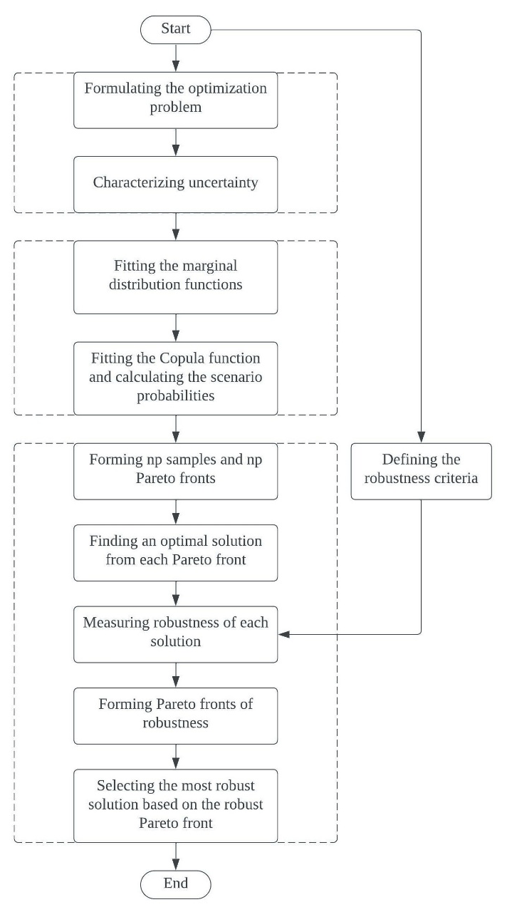
The specific process of optimal water allocation under runoff uncertainty based on the CM-ROPAR algorithm is as follows:

• Part 1 – analyzing the wet–dry encounters.

  1. Analyze the inflow wet and dry encounters. If the basin has k inflows, then there are 3^k wet–dry scenarios. For example, suppose there is one inflow in the upper and one in the middle reach of the basin. In that case, there are nine scenarios: wet–medium, wet–wet, medium–wet, medium–medium, medium–dry, dry–wet, dry–medium, and dry–dry.

  2. Choose a scenario from 1 to 3^k.

• Part 2 – sampling inflow.

  • 3.

    Based on the recorded annual inflow data Q, it is assumed that Q is not a definite value but that

    $$\begin{array}{}\text{(5)}& {\displaystyle }& {\displaystyle }Q=i_{\mathrm{uncertainty}}\cdot Q\text{(6)}& {\displaystyle }& {\displaystyle }{i}_{\mathrm{uncertainty}}\sim N\left(\mathit{\mu },{\mathit{\sigma }}^{\mathrm{2}}\right),\end{array}$$

    where i_uncertainty follows a normal distribution.

  • 4.

    For i=1 … np, sample the inflow.

  • 5.

    Sample u (inflow). As mentioned before, the uncertainty variable is obtained from the normal distribution N(μ,σ²). Assuming that the uncertainty variable follows N(1,0.0025), this represents a 99.74 % probability of the uncertainty variable falling within the interval [0.85, 1.15] and the inflow sample falling within the interval [$\mathrm{0.85}\cdot Q,\mathrm{1.15}\cdot Q$].

• Part 3 – forming the optimal solution set through np Pareto fronts.

  • 7.

    Select an ideal solution (IS) in each Pareto front F_r based on the distance to the origin point, forming the optimal solution set (set S).

• Part 4 – evaluate the robustness of each solution.

  • 8.

    Select a solution s_i (i=1 … np) from the solution set S.

  • 9.

    Put the inflow case u_r (r=1 … np) into s_i, and calculate P_r(u_rs_i) and WD_r(u_rs_i), respectively, to form 1200 values of P_r and WD_r (r=1 … np).

  • 10.

    Select the robustness evaluation criteria, RC1, RC2, RC3, and RC4.

  • 11.

    For each s_i (i=1 … np), calculate RC1, RC2, RC3, RC4, and SRI (system robustness indicator) corresponding to P_r and WD_r, respectively. Plot the corresponding graphs, and find the Pareto front of each graph.

  • 12.

    Find the solution with the highest robustness.

2.3 Defining the robustness criteria

According to the general definition of robustness, four common robustness criteria (RC) were used in this study (Beyer and Sendhoff, 2007). These must be minimized to achieve the maximum robustness of the solution, so the lower the criteria, the higher the robustness.

For the four RC, two MOO are implicitly defined, and optimization can be named the “two-layer multi-objective optimization of robustness criteria” (TL-MOORC). It is worth noting that TL-MOORC differs from the problem's MOO. A one-layer MOORC is a solution that may not be minimized at all four RC simultaneously. This problem can be solved by aggregating the four RC into one, for example, using a linear weighted combination. The second layer of MOORC is that for the two objective functions of a solution, the RC for both objective functions may not be minimized at the same time. Therefore, a trade-off must be made between the RC for the two objective functions.

The first of the RC is the expected value of each objective function, denoted as RC1. It reflects the fact that we want to find a solution that is good on average across all uncertainties and can be represented by

$$\begin{array}{}\text{(7)}& \mathrm{RC}\mathrm{1}\left(s\right)=\underset{N(s,u)}{\int }f(s,u)p\left(u\right)\mathrm{d}u,\end{array}$$

where p(u) is the probability density function of the uncertain variable u; it is the neighborhood of the solution s.

The second of the RC is the “worst case” (or “minimax” case), denoted as RC2. This robustness criterion is related to robustness because we want to find a solution s such that the value of each objective function in the worst case is the minimum possible. It can be presented as follows:

$$\begin{array}{}\text{(8)}& \mathrm{RC}\mathrm{2}\left(s\right)=\min \left(\right(f(s,u)\left)\right).\end{array}$$

The third of the RC is the standard deviation of each objective function, denoted as RC3. RC3 is related to the robustness of each objective function because we want to find a solution s such that the value of the objective function would not vary too much due to uncertainty. It can be expressed as follows:

$$\begin{array}{}\text{(9)}& \mathrm{RC}\mathrm{3}\left(s\right)=\sqrt{\underset{N(s,u)}{\int }\left(f\right(s,u)-f(u\left){)}^{\mathrm{2}}p\right(u)\mathrm{d}u}.\end{array}$$

The fourth of the RC is the “probabilistic threshold”, denoted as RC4. We want to find a solution s that minimizes the probability that the objective function is higher than the threshold of interest q. This criterion is usually associated with the reliability of the system. It can be expressed as follows:

$$\begin{array}{}\text{(10)}& \mathrm{RC}\mathrm{4}\left(s\right)=\mathrm{Pr}\left(f\right(s,u)>q\mathrm{|}s).\end{array}$$

In order to evaluate the integrated robustness of the water resources allocation scheme, the weighted sum of the four normalized RC (NRC_i) in this study was used as the integrated robustness criteria. In this study, we consider the four RC to be of equal importance, so all four indicators are given a weight of $\frac{\mathrm{1}}{\mathrm{4}}$.

$$\begin{array}{}\text{(11)}& \mathrm{SRI}={\displaystyle \frac{\mathrm{1}}{\mathrm{4}}}\mathrm{NRC}\mathrm{1}+{\displaystyle \frac{\mathrm{1}}{\mathrm{4}}}\mathrm{NRC}\mathrm{2}+{\displaystyle \frac{\mathrm{1}}{\mathrm{4}}}\mathrm{NRC}\mathrm{3}+{\displaystyle \frac{\mathrm{1}}{\mathrm{4}}}\mathrm{NRC}\mathrm{4}.\end{array}$$

(Of course, other methods of aggregation can be considered as well.)

2.4 Construction of the WRA model

2.4.1 Objective function

1. The availability of water for all sectors is an important social goal, so it is important to calculate the water deficit (WD):

   $$\begin{array}{}\text{(12)}& \min f_{\mathrm{1}}\left(Q\right)=\sum _{j=\mathrm{1}}^J\sum _{k=\mathrm{1}}^K{\left({\displaystyle \frac{D_{jk}-\sum _{t=\mathrm{1}}^T\sum _{i=\mathrm{1}}^I{Q}_{ijkt}}{D_{jk}}}\right)}^{\mathrm{2}},\end{array}$$

   where D_jk denotes the water demand of the water consumption department k of the city j, and Q_ijkt is the water supply quantity of the water source i to the water consumption department k of the city j in the period t.

2. As an ecological goal, pollution (P) is calculated as follows:

   $$\begin{array}{}\text{(13)}& \min f_{\mathrm{2}}\left(Q\right)=\sum _{j=\mathrm{1}}^J\sum _{k=\mathrm{1}}^K{d}_{jk}{p}_{jk}\sum _{i=\mathrm{1}}^I\sum _{t=\mathrm{1}}^T{Q}_{ijkt},\end{array}$$

   where d_jk denotes the representative pollutant discharge per unit of wastewater of the water department k of the calculation unit j (t m⁻³), and p_jk represents the sewage discharge coefficient of the water consumption department of the calculation unit. Q_ijkt is the water supply quantity of the water source i to the water consumption department k of the calculation unit j in the period t.

2.4.2 Constraints

1. The water demand constraint is calculated by

   $$\begin{array}{}\text{(14)}& \sum _{i=\mathrm{1}}^I\sum _{t=\mathrm{1}}^T{Q}_{ijkt}\le D_{jk}.\end{array}$$

2. The water supply capacity constraint is calculated by

   $$\begin{array}{}\text{(15)}& \sum _{k=\mathrm{1}}^K\sum _{j=\mathrm{1}}^J\sum _{t=\mathrm{1}}^T{Q}_{ijkt}\le U_i.\end{array}$$

3. The water resources constraint is calculated by

   $$\begin{array}{}\text{(16)}& \sum _{j=\mathrm{1}}^J\sum _{k=\mathrm{1}}^K{Q}_{ijk}\le {\mathrm{WR}}_i.\end{array}$$

3 Study area overview

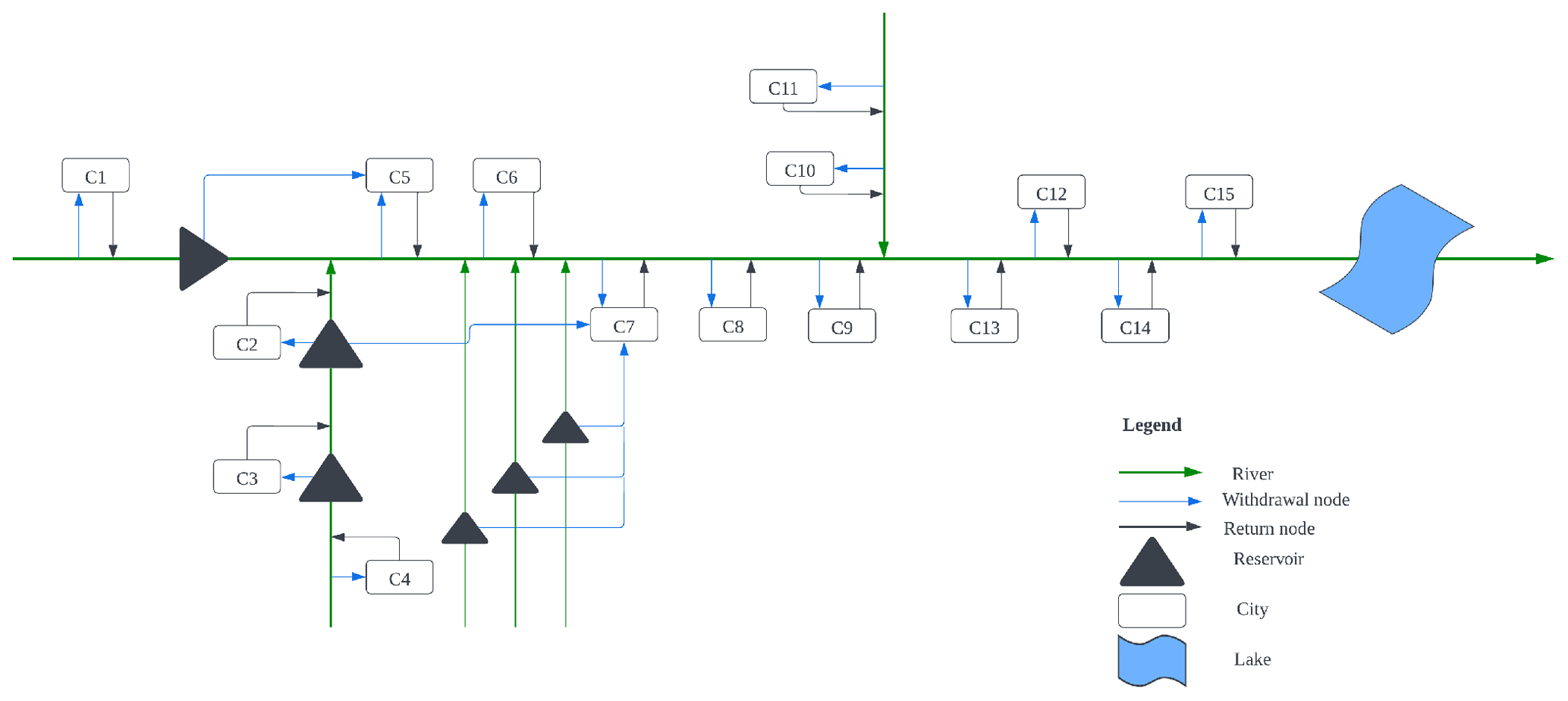
The Huaihe River basin is located in the eastern part of China, and as shown in Fig. 2, the midstream and upstream flow through 15 cities of Henan Province and Anhui Province. This is an important agricultural and industrial production base in China (Xu et al., 2019). As shown in Fig. 3, the inflow of the Huaihe River basin varies significantly between different years and between different regions, and the water demand is uneven among cities. In this study, water demand is calculated using the quota method commonly used in the field of water resources. In addition, due to the discharge of pollutants, the contradiction between supply and demand of water resources in the middle and upper reaches of the Huaihe River basin has become increasingly strong. Therefore, it is meaningful to study the optimal allocation of water resources and propose a robust water resources allocation scheme based on the wet–dry encounters in the Huaihe River basin.

Figure 2 Overview of watershed water supply.

Figure 3 Water demand proportion and inflow historical data.

4 Results and discussion

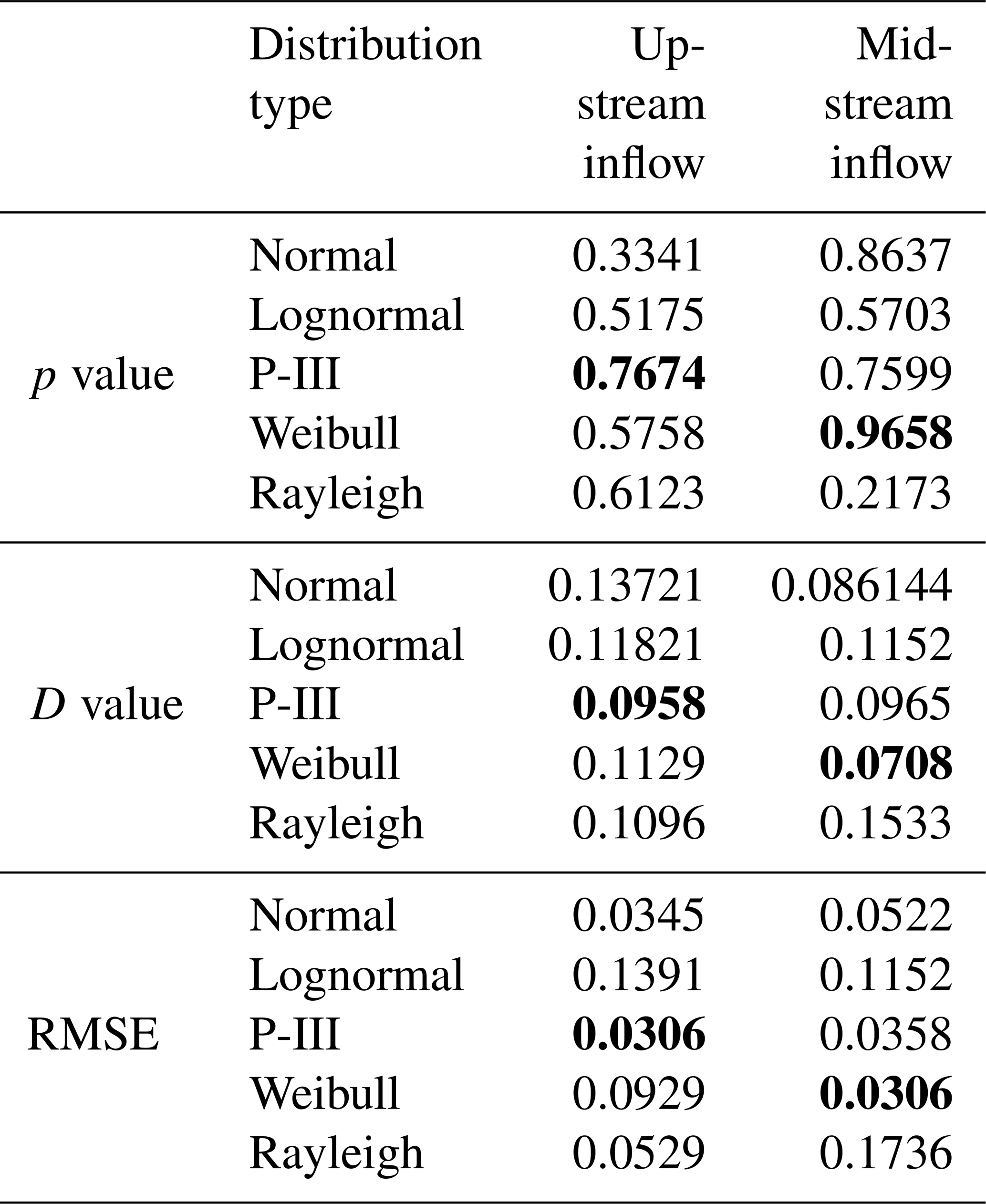
4.1 Identification of marginal distribution functions

According to the first part (step 1–2) of the CM-ROPAR process, we need to construct the joint probability distributions for the upstream and midstream inflow and generate nine inflow scenarios via the copula function. Therefore, before constructing the JDF, we need to construct the MDF for the upstream and midstream inflows, respectively. As shown in Table 1, based on the K–S test results and RMSE value, we found that the best-fitting distributions for the upstream and midstream were the Weibull and P-III distributions, respectively.

Table 1 MDF goodness-of-fit test results. Bold values indicate the distribution function with the best fit for this metric.

4.2 Analysis of upstream and midstream dry and wet encounters

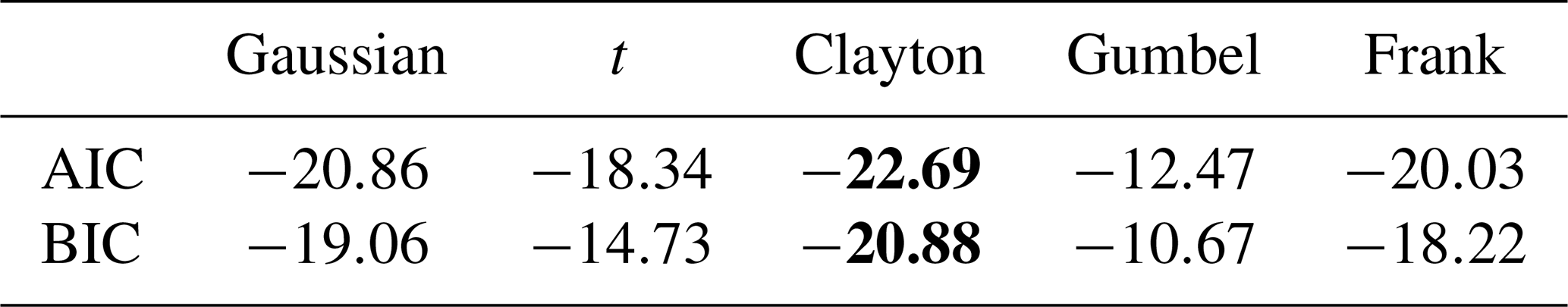
The optimal copula function is selected by comparing the Akaike information criterion (AIC) and the Bayesian information criterion (BIC) values shown in Table 2. It can be concluded that the joint distribution function of the upper and middle reaches of the Huaihe River basin is consistent with the joint distribution of the Clayton copula function.

Table 2 AIC and BIC values for copula functions. Bold values indicate the distribution function with the best fit for this metric. t denotes the t distribution.

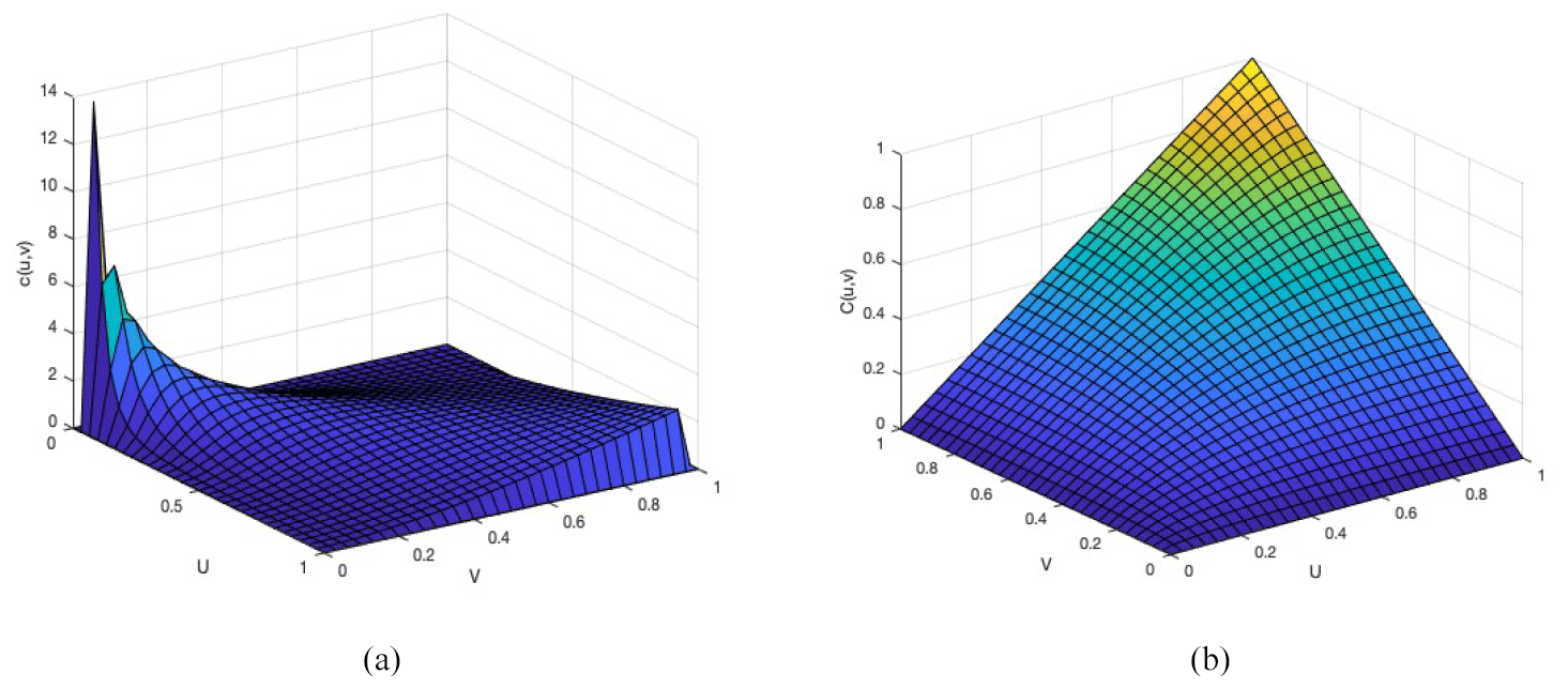
Substituting the multi-year annual inflow for the upper and middle reaches of the Huaihe River basin into the Clayton copula function, respectively, the following results were obtained.

As shown in Fig. 4, the joint distribution of the annual incoming water in the upper and middle reaches of the Huaihe River basin has symmetry. In addition, the joint distribution of annual water in the upper and middle reaches has a tail correlation, which indicates a higher probability of simultaneous wetness or drought in the upper and middle reaches.

Figure 4 Clayton copula function.

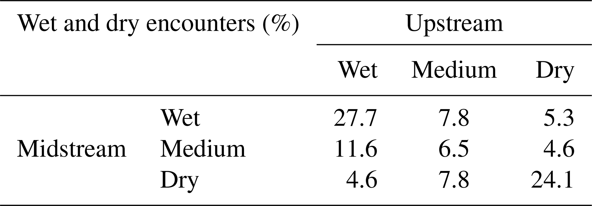
As shown in Table 3, the probability of drought–wetness synchronization in the upper and middle reaches of the Huaihe River basin is 58.3 %, while the probability of asynchrony is 41.7 %. The former is 16.6 % higher than the latter, indicating that the upper and middle reaches are less able to complement each other. The joint distribution has a maximum probability of 27.7 % that the upstream and midstream are both wet, and the risk of water scarcity is minimal under this scenario. The joint distribution has the second-highest probability of both upstream and midstream reaches being dry at 24.1 %, with the highest risk of water scarcity under this scenario.

Table 3 The probabilities of nine scenarios.

4.3 Considering solutions for the uncertainty of inflow through CM-ROPAR

In this study the situation when the upper and middle reaches are both wet is regarded as a case study. For deterministic optimization, we opted for the NSGA-II algorithm, which is widely used and has good historical performance (Reed et al., 2013). Inflow uncertainty is modeled by sampling 1200 inflows, as shown in Fig. 5. In this study, the NSGA-II algorithm is used for multi-objective function solving. For algorithm parameterization, the population size is 100, generation is 1000, the cross rate is 0.9, and the mutation rate is 0.2.

Figure 5 Inflow samples.

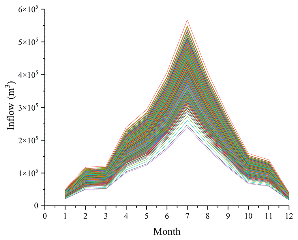
Figure 6a shows that 1200 Pareto fronts were calculated for each sampled inflow, through steps 3–6 of CM-ROPAR. Figure 6b shows 1200 ideal solutions s, selected based on their distance to the ideal solution (step 7 of CM-ROPAR).

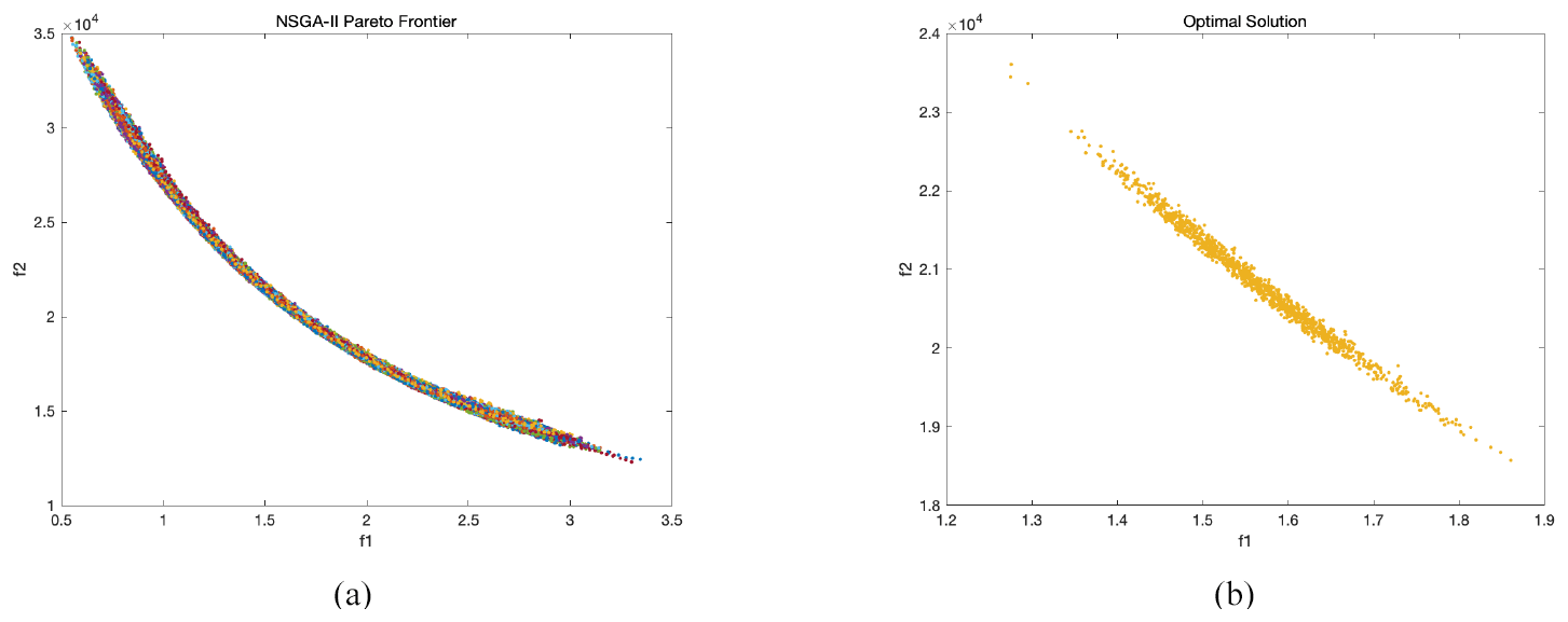
Figure 6 (a) 1200 Pareto fronts (f1, water deficit, and f2, pollution) and (b) 1200 ideal solutions (f1, water deficit, and f2, pollution) selected based on their distance to the ideal solution.

4.4 Assessing robustness of the solutions found by CM-ROPAR

Four robustness criteria are calculated for each solution s in the solution set S. Given the solution s to be evaluated, it is necessary to calculate $\mathrm{WD}(s,{\mathrm{IF}}_{\mathrm{r}})(r=\mathrm{1}\mathrm{\dots }np)$ and $P(s,{\mathrm{IF}}_{\mathrm{r}})(r=\mathrm{1}\mathrm{\dots }np)$ in order to calculate the four robustness criteria, where IF_r is the rth sample of inflow. r depends on the number of samples; in this study, 1200 samples were taken, so np is 1200.

As shown in Table 4 and Fig. 7, RC1, RC2, RC3, RC4, and SRI for WD and P can be calculated for each solution in S, and the solutions corresponding to the smallest value in each RC_i and the solutions corresponding to the smallest value in SRI can be identified, respectively. In addition, we also feed 1200 samples to the deterministic solution and calculate RC1, RC2, RC3, RC4, and SRI for WD and P.

Table 4 Optimal solution numbers for different robustness criteria.

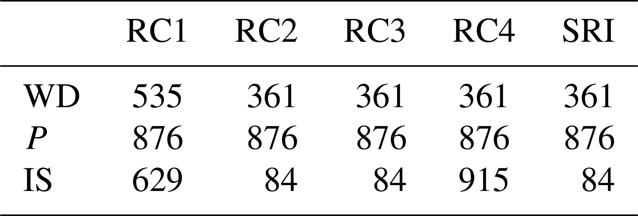
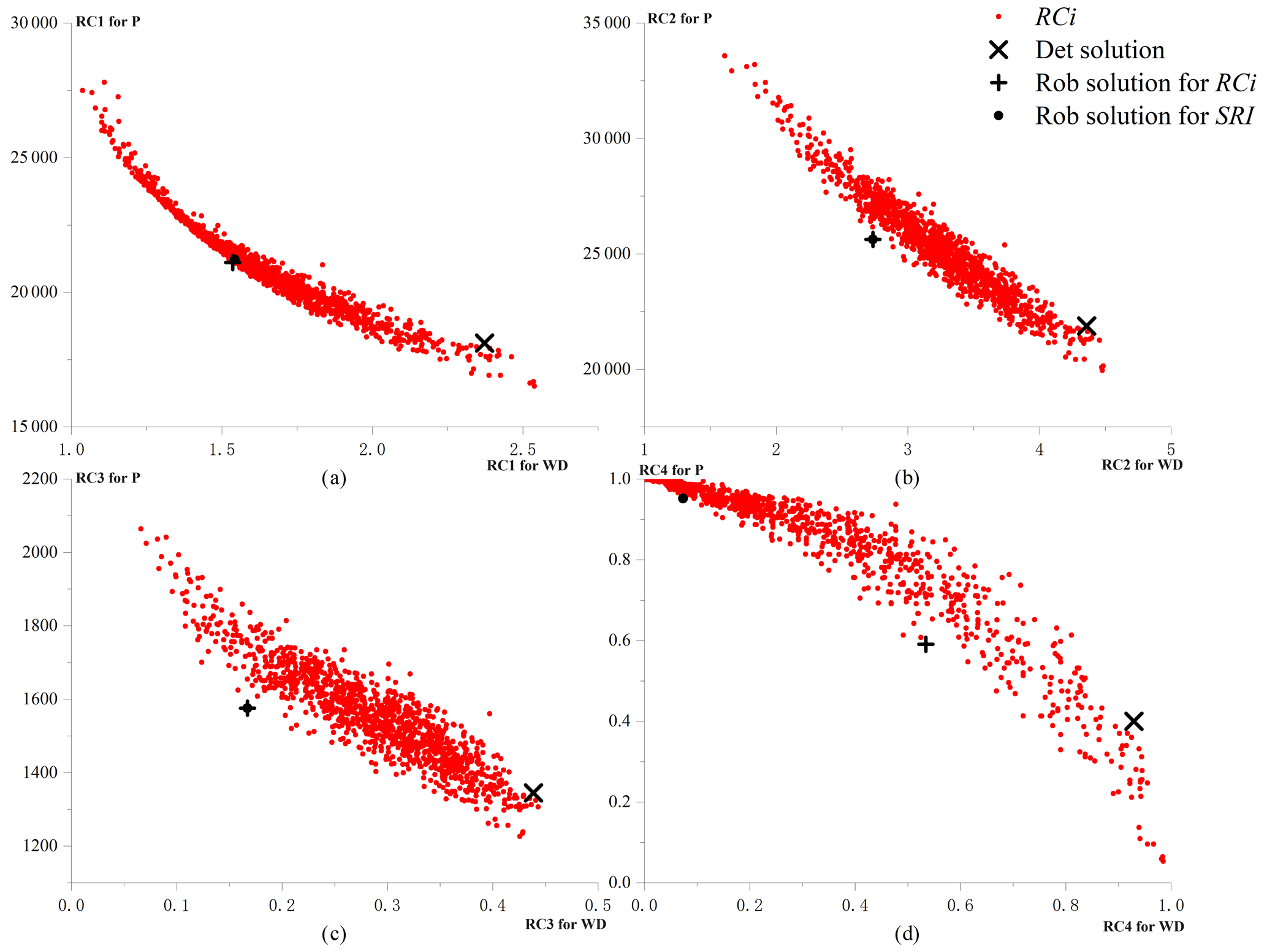
Figure 7 Performance of the robustness of solutions. (a) RC1, (b) RC2, (c) RC3, and (d) RC4 robust model solutions (red dots); deterministic model solution (black cross); solution closest to origin for RC_i (black plus symbol); and solution closest to origin for SRI (black dot). The horizontal axis represents the performance of the robustness for WD. The vertical axis represents the robustness performance for P.

Figure 7 shows the performance of 1200 robust model solutions (red dots) and one deterministic model solution (black ×), for the four robustness criteria. From Fig. 7, four Pareto fronts can also be found, which indicate the competitive relationship between water deficit and pollution emissions for each robustness criterion dimension. As shown in Fig. 7a, we can observe an interesting phenomenon that the left-most extreme solution (red dot) has the smallest robustness index RC1 for water deficit but the highest robustness index RC1 for pollution; the right-most extreme solution (red dot) has the largest robustness index RC1 for water deficit but the smallest robustness index RC1 for pollution. Similarly, this phenomenon can be also observed for the robustness criteria RC2, RC3, and RC4. More importantly, as shown in Table 4, the extreme solutions and the solutions closest to the origin point may differ for different robustness criteria. Specifically, for RC1, solution no. 535 is the most robust for water deficit, and solution no. 876 is the most robust for pollution; for RC2, RC3, and RC4, the most robust solution for water deficit is solution no. 361, and the most robust solution for pollution is solution no. 876.

Because there are many non-inferior solutions in the Pareto frontier, decision-makers must choose among them. Decision-makers need not only to choose among the non-inferior solutions but also to evaluate the trade-off between different robustness criteria or to choose the best one by combining the criteria. This study takes the distance to the origin as the basis for such a choice. As shown in Table 4, for RC1, RC2, RC3, and RC4, the closest points to the origin are solution no. 629, solution no. 84, and solution no. 915, respectively.

4.5 Comparing solutions found by deterministic and robust approaches

To see a more general relationship between the 1201 solutions (i.e., 1200 from the robust optimization solution and 1 from the deterministic optimization solution), the performance of each solution for water deficit and pollution for each of the four robustness criteria (sorted from smallest to largest) is plotted in Figs. 8 and 9.

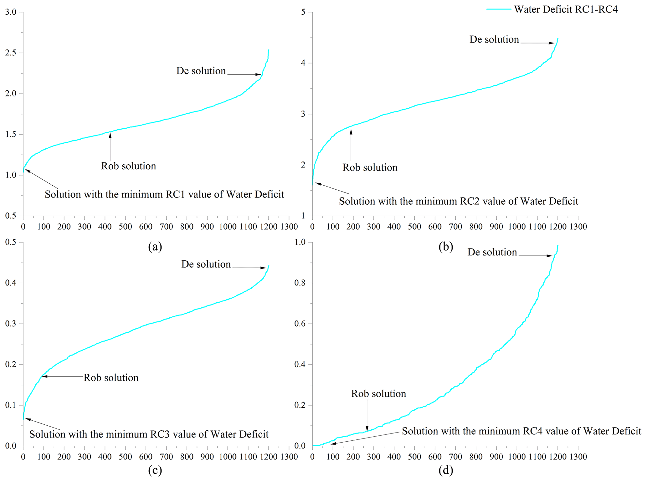
Figure 8 Robustness of water deficit for (a) RC1, (b) RC2, (c) RC3, and (d) RC4. The horizontal coordinate represents the number of solutions, and the vertical coordinate represents the robustness of the solution.

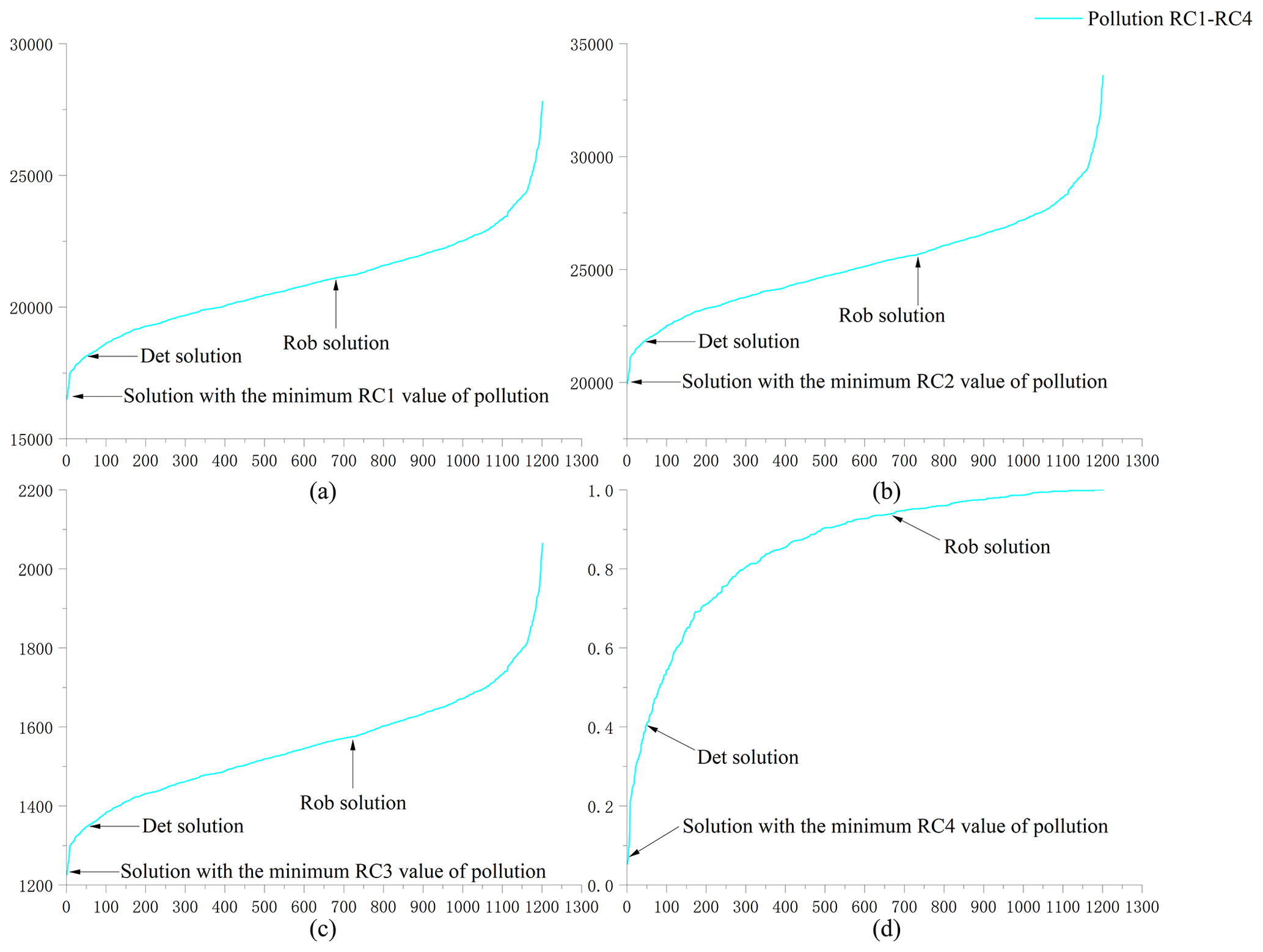
Figure 9 Robustness of pollution for (a) RC1, (b) RC2, (c) RC3, and (d) RC4. The horizontal coordinate represents the number of solutions, and the vertical coordinate represents the robustness of the solution.

As shown in Fig. 8, for water scarcity, the robust solution performed significantly better than the deterministic solution. Specifically, for the four robustness criteria, the robust solution outperforms 63.1 %, 85.6 %, 92.7 %, and 77.7 % of the solutions, respectively, while the deterministic solution outperforms only approximately 1 % of the solutions. To analyze the robust and deterministic solutions more accurately and intuitively, this study applied the ratio of $\mathrm{RC}\left(\mathrm{Det}\right)/\mathrm{RC}\left(\mathrm{Rob}\right)$ to compare the robustness of the two solutions. The ratios of $\mathrm{RC}\left(\mathrm{Det}\right)/\mathrm{RC}\left(\mathrm{Rob}\right)$ are 1.53, 1.59, 2.62, and 12.67 in the four robustness criteria dimensions. This means that, regarding water deficit, the deterministic model solution may lead to 53 %, 59 %, 162 %, and 1167 % more variability in the four robustness criteria dimensions.

However, as shown in Fig. 9, the deterministic solution slightly outperforms the robust solution for pollution. Specifically, for the four robustness criteria, the deterministic solution outperforms 96 % of the solutions, respectively, while the robust solution outperforms about 40 % of the solutions. Similarly, we compare the two solutions by the ratio of $\mathrm{RC}\left(\mathrm{Rob}\right)/\mathrm{RC}\left(\mathrm{Det}\right)$. We find that the $\mathrm{RC}\left(\mathrm{Rob}\right)/\mathrm{RC}\left(\mathrm{Det}\right)$ ratio is about 1.17 for RC1 to RC3 and 2.37 for RC4. This means that, in terms of pollution, the robust solution may lead to 17 % more variability for RC1 to RC3 and 137 % more variability for RC4.

In order to analyze the comprehensive performance of each solution, rather than just the robustness of a single objective, this study reflects the comprehensive implementation of each solution in terms of the distance from the solution to the origin. As shown in Fig. 10, the comprehensive performance of the robust solution for RC1 to RC4 is significantly better than that of the deterministic model solution. Specifically, the robust solution outperforms 90.3 % and 62.2 % of the solutions in RC1 and RC4, respectively, and outperforms all solutions in RC2 and RC3, while the deterministic solution performs exceptionally poorly in all four robustness criteria. According to the ratio of $\mathrm{Dis}\left(\mathrm{Rob}\right)/\mathrm{Dis}\left(\mathrm{Det}\right)$, we find that the robust solution is 16.8 %, 19.8 %, 39.2 %, and 7.3 % more robust than the deterministic solution in the four robustness dimensions, respectively.

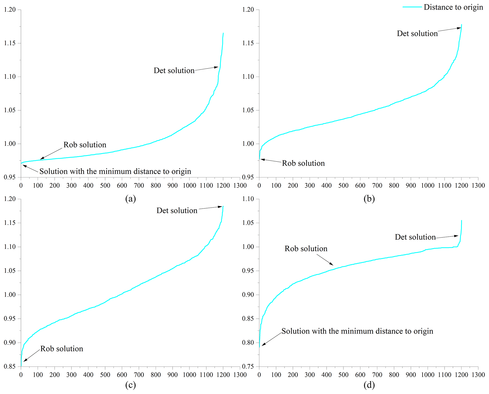
Figure 10 Comprehensive robustness for four indicators, (a) RC1, (b) RC2, (c) RC3, and (d) RC4. The horizontal coordinate represents the number of solutions, and the vertical coordinate represents the robustness of the solution.

As shown in Fig. 11, for water scarcity, the integrated criteria of the robust solution are clustered at approximately 0.5 and are significantly more robust than the deterministic solution; for pollution, the integrated index of the robust solution is significantly higher than that of the deterministic solution, but the span of the integrated index of the two solutions is similar, so the robustness of the deterministic solution is slightly better than that of the robust solution.

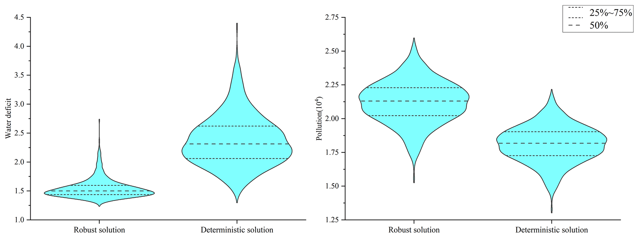
Figure 11 The integrated robustness index distribution of the robust and deterministic solution.

Similarly, as shown in Fig. 12, there is also a Pareto front for the composite robustness criteria. For water deficit, the robustness of the robust solution is better than the deterministic solution; for pollution, the robustness of the deterministic solution is better than the robust solution. Specifically, for water deficit, the robust solution outperforms 85.3 % of the solutions, while the deterministic solution outperforms only about 1 % of the solutions; for pollution, the deterministic solution outperforms 96 % of the solutions, while the robust solution outperforms only 39.6 % of the solutions. According to the ratio of $\mathrm{SRI}\left(\mathrm{Rob}\right)/\mathrm{SRI}\left(\mathrm{Det}\right)$, the deterministic solution is about 130 % more uncertain than the robust solution for water deficit; for pollution, the robust solution is about 37.7 % more variable than the deterministic solution. The distance of each solution to the origin can reflect the comprehensive performance of the robustness of each solution. For the robustness composite index, the ratio of $\mathrm{Dis}\left(\mathrm{Rob}\right)/\mathrm{Dis}\left(\mathrm{Det}\right)$ is 0.655, which means that the composite robustness of the robust solution is 52.6 % higher than the robustness of the deterministic solution.

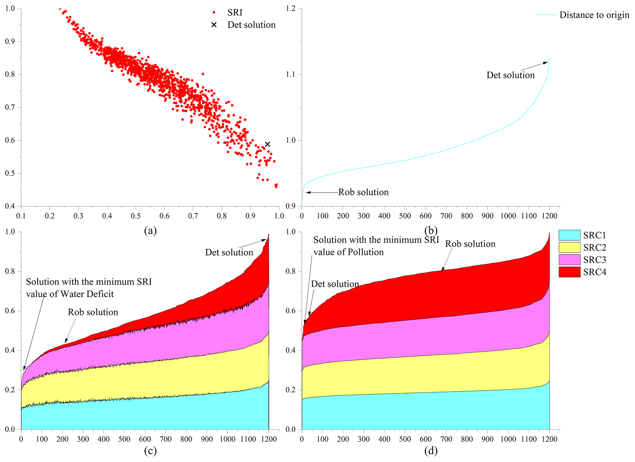
Figure 12 Comprehensive robustness criteria performance. (a) Performance of comprehensive robustness criterion. (b) Comprehensive robustness of robust solutions and deterministic solution. (c, d) Comprehensive robustness criteria for water deficit and pollution.

For the robustness composite, the robust solution outperforms all the solutions, while the deterministic model solution outperforms only about 3.2 % of the solutions. Comparing the distance to the origin of the robust solution and the deterministic solution, we find that the robustness of the robust solution improves by 27.8 % over the deterministic solution.

4.6 Analysis of specific water resources allocation schemes

First, as shown in Fig. 13, we analyzed the proportion of water supply for each city. We find that the water supply share for the scheme most robust to water deficit rates is significantly higher than that for the scheme with the most robust pollutant emissions. This is because an increase in water supply leads to an increase in pollutant emissions, which in turn leads to a decrease in the robustness of pollutant emissions. For specific cities, the least robust allocation scheme for water deficit reduces the water supply in City 3, City 7, City 10, City 12, and City 15 compared to the most robust allocation scheme for pollutant emissions. Interestingly, these cities have the most water demand in the basin (as shown in Fig. 3). Therefore, basin managers can increase the water supply to these cities if they need to improve the water deficit robustness of the water resources allocation scheme.

Figure 13 Specific water resources allocation schemes.

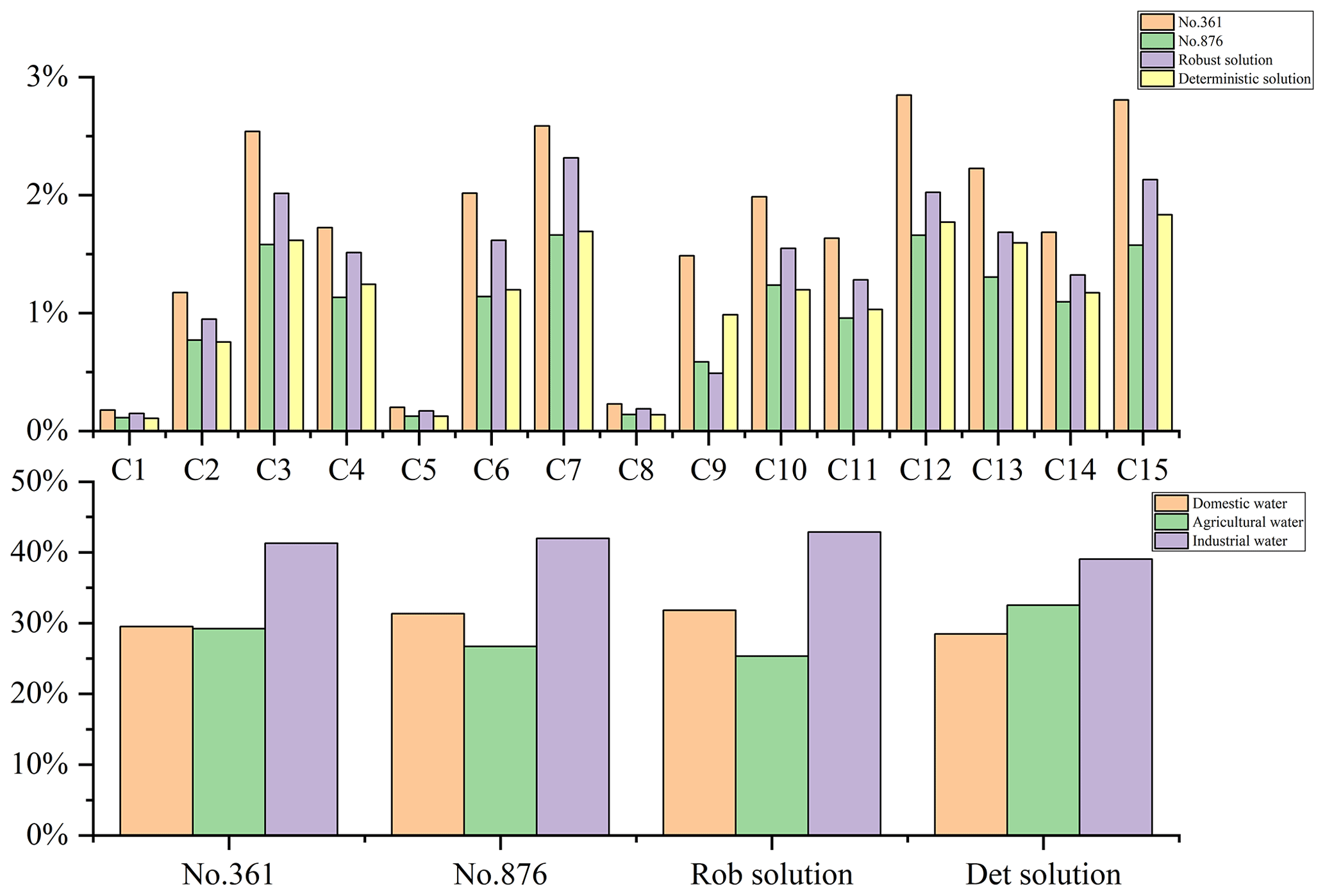
Then we analyze specifically the distribution of water resources between sectors. An interesting phenomenon is observed. As shown in Fig. 13, although the scenario with the best robustness in terms of pollutant emissions has a lower water supply than the scenario with the best robustness in terms of water deficit, the reduction is mainly in the agricultural sector. Water for domestic and industrial production did not change much. The reason for this may be that agricultural water use causes more pollution and may create more uncertainty. Therefore, now watershed managers hope that improving the robustness of pollutant discharge can reduce water supply to the agricultural sector.

5 Conclusion

In this study, we propose a multi-objective robustness analysis method considering multiple uncertainties (CM-ROPAR approach) based on the robust optimization method for uncertainty perception (ROPAR approach). To verify the superiority and practicality of the CM-ROPAR approach, four robustness criteria are selected, and we compare the robust solution calculated by the method with the optimal solution of the deterministic model. In the studied case, there is a competitive relationship between the robustness of the two objective functions, which can form a Pareto frontier. For the water deficit rate, the robust solution outperforms the deterministic solution by 53 %, 59 %, 162 %, and 1167 % for the four robustness criteria, respectively; for the pollutant emission, the deterministic solution outperforms the robust solution by only 17 % for RC1–RC3 and outperforms the robust solution by 137 % for RC4. For the composite robustness, the robust solution outperforms the deterministic solution by 52.6 %; CM-ROPAR finds a more robust solution.

The CM-ROPAR approach shows how uncertainty is handled, to be able to analyze how uncertainty is transmitted to the Pareto frontier and to perform the corresponding probabilistic analysis. The novelty of the new method compared to existing ROPAR methods is reflected in two aspects. First, the ROPAR method only considers uncertainty at a single point. In contrast, the CM-ROPAR method considers multiple uncertainties through the joint probability distribution of two points, which is closer to the actual situation and more general. Second, the new method analyzes the robustness of two objective functions of the solution instead of fixing one objective function to analyze the robustness of the other objective function. The CM-ROPAR method is more comprehensive and can identify the robustness of both objective functions, giving decision-makers more information for decision-making.

One of the limitations of this study is that the CM-ROPAR approach is applicable to problems with two uncertainties and two objective functions; however, there are more uncertainties and more objective functions (e.g., the uncertainty of inflow between multiple tributaries) in water allocation. In future research, we will focus on more complex objective functions and multi-objective optimization problems with at least three objective functions.