Drainage assessment of irrigation districts: on the precision and accuracy of four parsimonious models

In semi-arid irrigated environments, agricultural drainage is at the heart of three agro-environmental issues: it is an indicator of water productivity, it is the main control to prevent soil salinization and waterlogging problems, and it is related to the health of downstream ecosystems. Crop water balance models combined with subsurface models can estimate drainage quantities and dynamics at various spatial scales. However, such models' precision (capacity of a model to fit the observed drainage using site-specific calibration) and accuracy (capacity of a model to approximate observed drainage using default input parameters) have not yet been assessed in irrigated areas. To fill the gap, this study evaluates four parsimonious drainage models based on the combination of two surface models (RU and SAMIR) and two subsurface models (Reservoir and SIDRA) with varying complexity levels: RU-Reservoir, RU-SIDRA, SAMIR-Reservoir, and SAMIR-SIDRA. All models were applied over two sub-basins of the Algerri–Balaguer irrigation district, northeastern Spain, equipped with surface and subsurface drains driving the drained water to general outlets where the discharge is continuously monitored. Results show that RU-Reservoir is the most precise (average KGE (Q^0.5) of 0.87), followed by SAMIR-Reservoir (average KGE (Q^0.5) of 0.79). However, SAMIR-Reservoir is the most accurate model for providing rough drainage estimates using the default input parameters provided in the literature.

1 Introduction

In the context of ongoing global changes, semi-arid irrigated areas, in particular, face multiple challenges. First, agricultural water productivity is a critical issue in regions where water resources are under increasing pressure (FAO, 2021). Second, one-third of the world's irrigated land is affected by the soil salinization issue, which is likely to bring a significant loss in terms of arable lands (Singh et al., 2019). Third, non-point pollution is another issue in irrigated areas, with return flows that may contain high concentrations of nutrients (García-Garizábal and Causapé, 2010) and/or pesticides (Abdi et al., 2021).

Agricultural drainage is at the heart of the above three challenges (water productivity, soil salinization, and non-point pollution). More than 20 % of the total irrigated lands in the world are equipped with drainage systems, including open ditches or buried drains (Schultz et al., 2007). Drainage systems are generally installed to prevent waterlogging during heavy rainfall (through a sudden rise in the water table), to facilitate salt leaching (particularly when the irrigation water has high salt concentrations), and to maintain a low water table to avoid salt accumulation by capillary rise in the root zone (particularly when the groundwater has high salt concentrations). Moreover, the drained water quantity and quality are strong indicators of agricultural water productivity and the possible impact of nitrates, salts, and pesticide concentration on downstream ecosystems (Blann et al., 2009).

Measuring drainage discharge is an effective way of monitoring the quantity and quality of drainage to help address the three challenges mentioned above. However, the proportion of drained irrigation districts equipped with such instruments is very low. In this context, estimating the drained water in irrigated areas, including those not instrumented, is of major importance. Some work has been done in this regard over rainfed areas, focusing on modeling the quantity and quality of the drained water discharged (e.g., Negm et al., 2017) or on developing drainage scenarios that integrate changes in agricultural practices (e.g., Tournebize et al., 2004) or in climatic conditions (e.g., Golmohammadi et al., 2020; Jeantet et al., 2022). However, only a few studies have dealt with the quantitative estimation of drainage in semi-arid irrigated areas. At the field scale, Ale et al. (2013) compared the ability of the physically based DRAINMOD (Skaggs et al., 2012) and ADAPT (Gowda et al., 2012) models to simulate monthly drainage in a drip-irrigated plot in the US. The determination coefficient between simulated and observed drainage was 0.90 and 0.85 for ADAPT and DRAINMOD, respectively, for data obtained over 7 years. More recently, Feng et al. (2021) simulated the daily drainage with the physically based Hydrus-2D model in a furrow-irrigated plot and obtained a Nash–Sutcliffe model efficiency coefficient (NSE) value of 0.91 and 0.94 for the calibration and validation years, respectively. At a larger spatial scale, Cavero et al. (2012) simulated the monthly drainage of three Mediterranean irrigated catchments (mainly surface irrigation) located in Spain, Algeria, and Turkey, ranging from 4000 to 10 000 ha. They used the crop water balance model APEX (Gassman et al., 2010) coupled with DRAINMOD over 2 hydrological years and obtained root-mean-square deviation (RMSD) values ranging from 3.4 to 25.3 mm per month. On a much larger scale, Wen et al. (2020) simulated the monthly drainage over 19 sub-basins in a 1.2×10⁶ ha irrigation district in northern China using an empirical approach based on water table observations. The results showed a mixed performance with an average NSE of 0.64 and a standard deviation of 0.21 for the 2-year calibration period and an average NSE of 0.34 and a standard deviation of 0.44 for the 2-year validation period. In the same irrigation district, Chang et al. (2021) simulated the annual drainage discharge under different management scenarios using the semi-empirical SahysMod model (Oosterbaan et al., 2005).

Although the literature on agricultural drainage is still limited for semi-arid irrigated areas, there are many scientific papers on drainage estimation in humid regions where waterlogging problems are common. The vast majority of them use physically based models such as DRAINMOD (Moursi et al., 2022; Muma et al, 2017), RZWQM2 (Ma et al., 2012; Xian et al., 2017; Jiang et al. 2020), MACRO (Larsbo et al., 2005; Jarvis and Larsbo, 2012), SWAP (van Dam et al., 2008), HydroGeoSphere (De Schepper et al., 2015), and FLUSH (Turunen et al., 2013; Nousiainen et al., 2015). Generally, these models are implemented at the plot scale and represent the intermediate processes (e.g., macropore infiltration, deep seepage, water redistribution in the soil profile, rooting distribution, lateral flows) involved in drainage at a daily or hourly time step. They rely on a lot of information for model parameterization, implying detailed knowledge of the studied site and potentially numerous parameters to calibrate. For example, Ma et al. (2012) recommend that, for the RZWQM2 model, there be an independent measurement for 11 parameters and a calibration for 11 others out of a total of 24 parameters (with the 2 remaining ones being taken from the literature). In fields where intensive measurement campaigns have been conducted, these models can simulate the observed drainage well at hourly, daily, weekly, or monthly scales. However, the application of such models to poorly monitored basins remains limited due to the need for site-specific calibration (using drainage measurements) to set their relatively numerous input parameters.

Henine et al. (2022) proposed a simple semi-empirical drainage model, RU-SIDRA, to generalize a drainage model for various agricultural conditions. It combines a surface model (RU) to simulate the daily recharge and a subsurface model (SIDRA) (Lesaffre and Zimmer, 1988; Bouarfa and Zimmer, 2000) to convert the simulated recharge into daily drainage discharge. RU is a water balance model based on a simplified version of the FAO-56 method (Allen et al., 1998) and relies only on a single sensitive parameter. SIDRA is based on the resolution of a semi-analytical formula derived from the Boussinesq physical equation (Boussinesq, 1904), leading to two main sensitive parameters. The robustness of RU-SIDRA was evaluated by Jeantet et al. (2021) on 22 non-irrigated French fields and sub-basins over 200 hydrological years. It was found that RU-SIDRA performs as well as physically based models in reproducing daily drainage and is as robust as the latter from one hydrological year to another. However, Jeantet et al. (2021) emphasized a limitation of RU-SIDRA associated with the empirical nature of the RU model. Indeed, in RU, the start of drainage, occurring in autumn in the non-irrigated sites studied by Jeantet al. (2021), is not systematically well reproduced from year to year. This is potentially due to its poor representation of the processes governing the variations in the soil water stock (e.g., root growth or evapotranspiration). Over irrigated areas, this difficulty is expected to be further exacerbated by the impact of summer crops. In addition, as with the physically based models described previously, RU-SIDRA also relies on a site-specific calibration step using rarely available observed drainage data.

Finding the right balance between the simplicity required for a drainage model to be easily applicable over large areas and the complexity needed to ensure sufficient realism in terms of intermediate processes and, hence, the robustness of drainage estimates in time remains challenging. In this context, this study seeks to address the following questions:

• Can parsimonious models with different degrees of complexity precisely reproduce the daily drainage in a semi-arid irrigated context with site-specific calibration?

• Can such models with default calibration (with parameter values provided in the literature) reproduce drainage quantities and dynamics, even roughly?

In this context, we evaluated the precision and accuracy of several parsimonious models based on the RU-SIDRA formalism. By precision and accuracy, we mean the capacity of each model to predict the drainage after site-specific calibration (using drainage measurements) and by setting the model input parameters to the default values found in the literature (without using drainage measurements), respectively. Precision evaluation aims to investigate the models' strengths and weaknesses by calibrating and validating them over the same period. The accuracy evaluation aims to determine (i) whether it is possible to estimate drainage when no in situ drainage data are available for calibration (which is the case for most irrigation districts), i.e., under non-optimal calibration conditions, and (ii) which of the models evaluated performs best under these conditions.

To cover a range of modeling complexities, we investigate the SAMIR model (Simonneaux et al., 2009) as an alternative to the RU model. SAMIR is more complex than RU as it simulates more processes (e.g., root growth, vegetation development, evaporation, vegetation cover, specific crop water needs, and stress resistance) while remaining parsimonious, with only two parameters integrating most of the sensitivity for the recharge simulation (Laluet et al., 2023). We also investigate the Reservoir model as an alternative to the SIDRA model. Reservoir is a fully empirical model driven by a single parameter. It is a simplified version of a module recently incorporated in the SASER (SAfran-Surfex-Eaudysee-Rapid) hydrological model (Quintana-Seguí et al., 2017; Vergnes and Habets, 2018; David et al., 2011) by Cenobio-Cruz et al. (2023), who showed its ability to satisfactorily reproduce the low flows (groundwater discharge) observed at 53 hydrological stations in France and Spain.

The combination of both recharge (RU and SAMIR) models and both subsurface (Reservoir and SIDRA) models generates four drainage models in the following order of increasing complexity: RU-Reservoir (two main parameters), RU-SIDRA (three main parameters), SAMIR-Reservoir (three main parameters), and SAMIR-SIDRA (four main parameters). In this study, the precision and accuracy evaluations of the four drainage models are carried out in two sub-basins of the Algerri–Balaguer irrigation district located in the Ebro basin in the northeast of Spain. These two sub-basins are instrumented with flow meters that continuously measure the daily drainage discharge into the main drains.

2 Material and methods

The overall methodology to assess both the precision and accuracy of RU-Reservoir, RU-SIDRA, SAMIR-Reservoir, and SAMIR-SIDRA is presented in the flowchart of Fig. 1. First, the study site and data used are presented (Sect. 2.1), followed by a description of the four models (Sect. 2.2). The following sections describe the site-specific calibration strategy used for evaluating the precision of the models (Sect. 2.3), the selection of input parameter ranges used for evaluating the accuracy of the models (Sect. 2.4), and their complexity of use (Sect. 2.5).

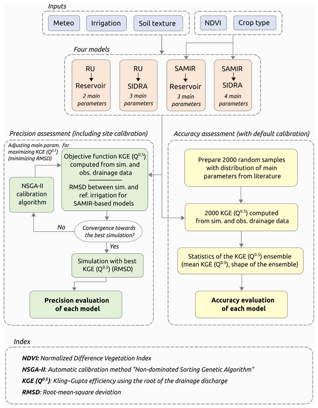
Figure 1 Flowchart of the proposed methodology for precision and accuracy evaluation of the drainage simulated by four parsimonious models with different levels of complexity.

2.1 Study area and data

2.1.1 Study area

The Algerri–Balaguer (AB) irrigation district is located in northeastern Spain, 20 km north of Lleida. It is characterized by a semi-arid continental Mediterranean climate with an average annual reference evapotranspiration (ET₀) of 1027 mm and precipitation of 380 mm (2000–2021). AB has an area of 8100 ha of cropland with mainly corn, barley, wheat, fruit trees, and alfalfa. A total of 6800 ha is equipped for irrigation with sprinklers for annual crops and drip systems for fruit trees. An overview of the AB area is shown in Fig. 2. For an extensive description of the irrigation district in terms of soil, geology, crops, irrigation, and drainage system, the reader is referred to Altés et al. (2022).

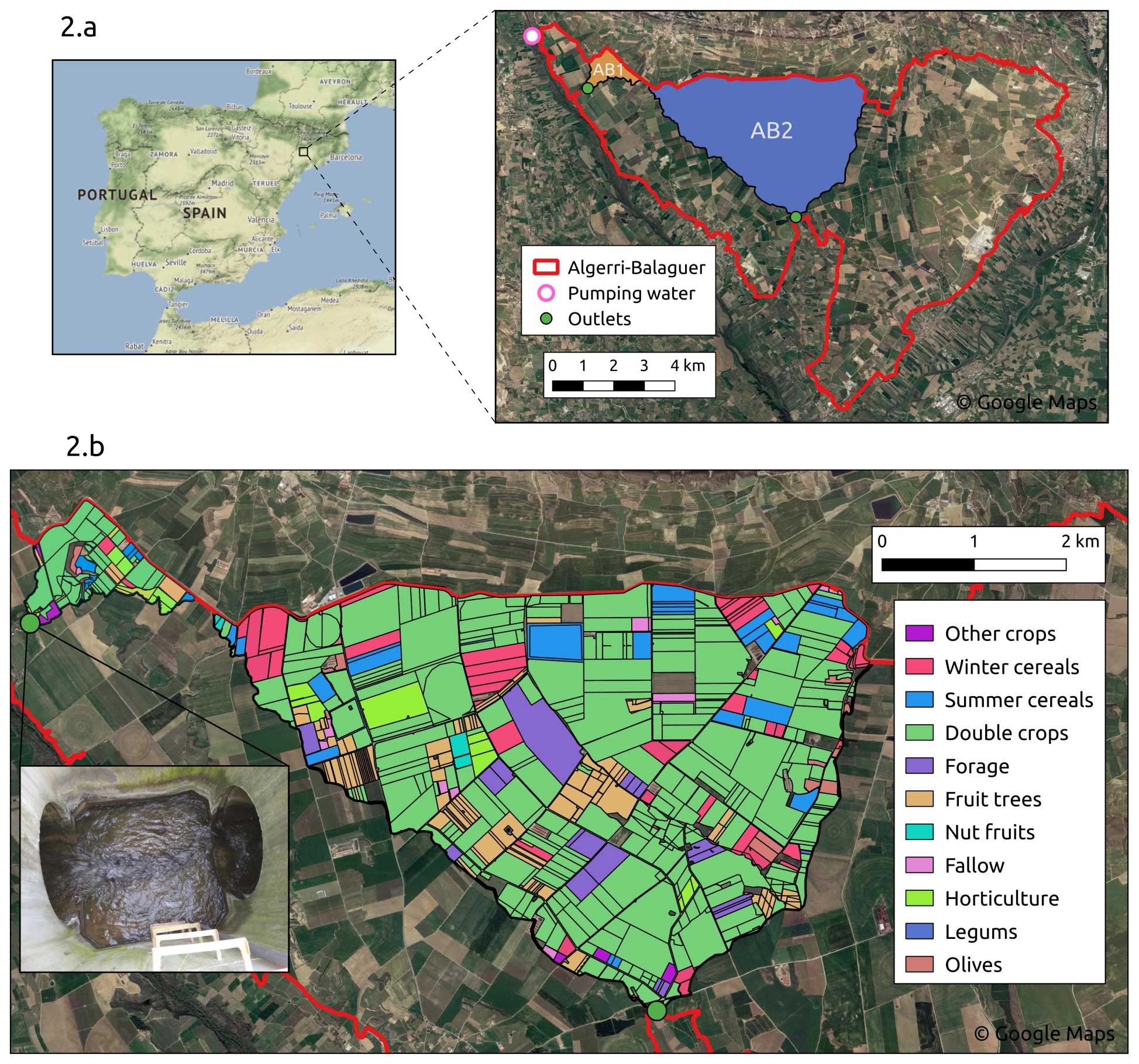
Figure 2 The AB irrigation district with the two monitored sub-basins, AB1 and AB2, and their outlets, as well as the location of the pumping station for irrigation (coordinates: 41.829° N, 0.579° E; WGS84) (a). Zoom on the two sub-basins with their land use for the year 2021 and a picture of the inside the AB1 outlet, where water level is measured before being converted into drainage discharge (b).

In 1998, modernization works were carried out in the AB district, including flattening the land for plot consolidation and installing irrigation systems and a drainage network. The drainage network consists of surface (open ditches) and subsurface (buried pipes) drains (Altés et al., 2022). Field drains (underground perforated plastic pipes) are connected to collectors (underground concrete pipes larger than field drains). These collectors, in turn, are connected to main drains (either larger underground concrete pipes or open ditches). The main drains ultimately convey the water to general outlets (green dots in Fig. 2). During irrigation implementation, the collectors and the main drains were installed in the first few years. Since then, field drains have been installed progressively at the initiative of each farmer according to their needs. We have no precise information on the surface that has been equipped with field drains or on their spacing. From field observations, we know that the surface drains were dug at a depth of approximately 2 m, as were the main drains.

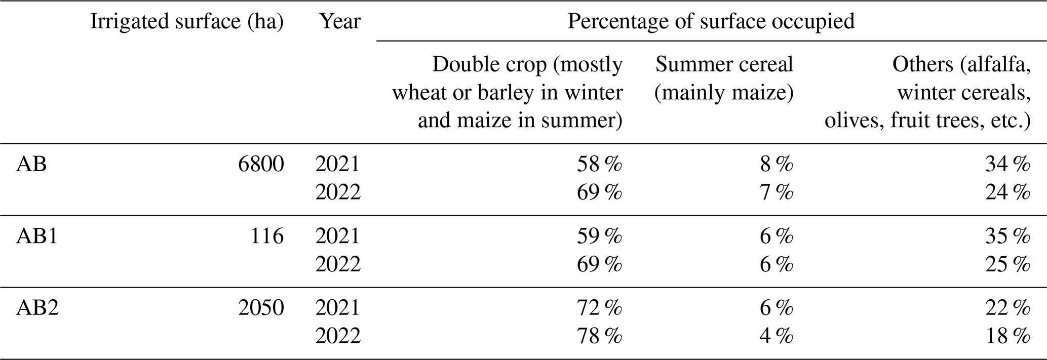
Two of these main drains have been equipped with CTD-10 sensors (Meter Group Inc., Pullman, WA, USA) that continuously measure the water level. They collect drainage water from areas of 116 and 2050 ha each, forming two sub-basins, AB1 and AB2 (see Fig. 2). These areas correspond to the topographic basins formed by the main drains at the CTD-10 sensor locations and were computed using the QGIS software with a 2 m resolution DEM provided by the Cartographic and Geological Institute of Catalonia. Table 1 shows, for AB, AB1, and AB2, the area and percentages of the main crop types. Figure 2b shows the land cover of AB1 and AB2 for 2021.

Table 1 Irrigated surfaces of AB, AB1, and AB2 and the percentage of surface area occupied by their different crop types in 2021 and 2022.

2.1.2 Description of the data used in this study

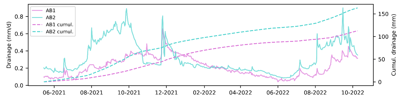
The water levels measured in the AB1 and AB2 outlets are obtained hourly and are converted into daily discharge using the Manning–Strickler equation and the knowledge of the main drain hydraulic characteristics (Altés et al., 2022). The available drainage data used herein cover the period from February 2021 to October 2022 (21 months) for AB1 and from May 2021 to October 2022 (18 months) for AB2. The observed drainage at AB1 was 29 mm in 2021 and 26 mm in 2022, while it was 61 mm in 2021 and 46 mm in 2022 at AB2. Figure 3 shows daily drainage data for AB1 and AB2 for the period May 2021 to October 2022.

The irrigation data consist of the daily flow of water pumped from a river next to the AB district (see Fig. 2), which is the only supply for the irrigation network. They are provided by the Automatic Hydrological Information System of the Ebro Basin (SAIH). Pumping flow data are aggregated to the weekly scale to consider the potential delay of several days between pumping and application in the field. A total of 5.8 % of the volume is removed to account for evaporation loss and leakage based on a comparison between the water pumped from the river and irrigation data from water meters (Olivera-Guerra et al., 2023).

Soil texture is obtained from the 250 m resolution SoilGrids product (Hengl et al., 2017; Poggio et al., 2021). It is relatively uniform over the AB area and corresponds to a silty clay loam soil (Jahn et al., 2006).

Meteorological data are obtained from five stations belonging to the Catalan Meteorological Station Network. Two are located within the AB district, and the three others are located around the area at a maximum distance of 5 km. The mean and standard deviation of the instantaneous measurements of precipitation and ET₀ made by the five stations are very low. Therefore, the spatial average of precipitation and ET₀ measurements is used as forcing at the scale of the AB sub-basins.

Figure 3 Bottom: daily drainage data of AB1 and AB2 from May 2021 to October 2022.

2.2 Description of the four models

The four models evaluated herein result from the combination of two water balance models (RU and SAMIR) and two drainage discharge models (Reservoir and SIDRA). Their main characteristics are listed in Table 2.

Table 2 Description of the four models used.

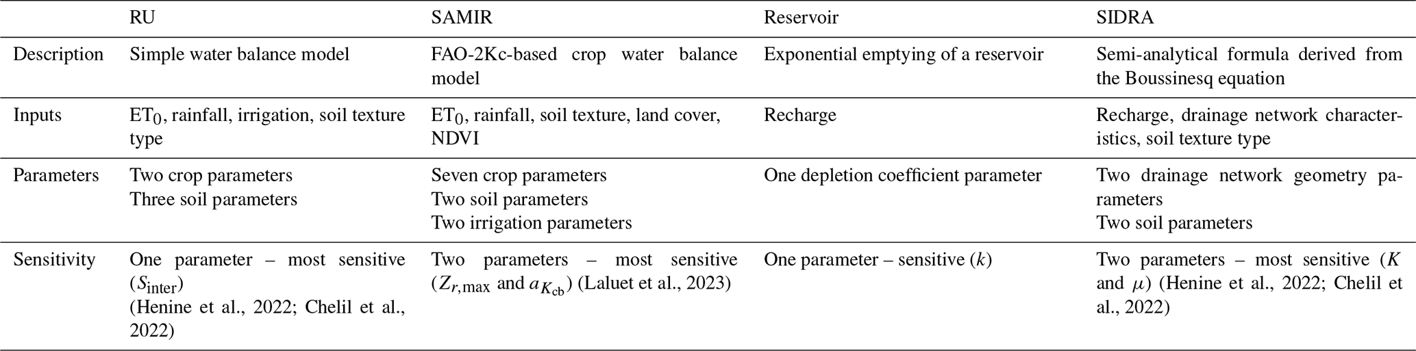
2.2.1 SAMIR

The SAMIR model (Simonneaux et al., 2009) is a FAO-56 double-crop coefficient-based model (FAO-2Kc) (Allen et al., 1998) designed to simulate the crop water balance components for daily ET estimation and crop water requirements by considering the plant and soil water status. It uses (i) meteorological forcing variables to calculate ET₀ (calculated using the Penman–Monteith equation); (ii) precipitation; (iii) crop and soil parameters to calculate soil reservoir properties, as well as plant and soil resistance to water stress; and (iv) normalized difference vegetation index (NDVI) to drive plant development, obtained from the Sentinel-2 satellites with a resolution of 10 m and a revisit time of 5 d.

The daily water balance equation simulated with SAMIR is as follows:

$$\begin{array}{}\text{(1)}& {D_{\mathrm{r}}}_t={D_{\mathrm{r}}}_{t-\mathrm{1}}+{\mathrm{ET}}_t-P_t-I_t+R_t,\end{array}$$

where D_r is the root zone depletion, ET is the actual evapotranspiration, P is the precipitation, I is the irrigation, and R is the underground recharge. Every term is expressed in millimeters for the day t (and t−1 for D_r). ET is estimated by multiplying two crop coefficients to ET₀ as follows:

$$\begin{array}{}\text{(2)}& {\mathrm{ET}}_t=\left({K_{\mathrm{cb}}}_t\cdot K_{\mathrm{s},t}+K_{\mathrm{e},t}\cdot K_{\mathrm{r},t}\right)\cdot {\mathrm{ET}}_{{\mathrm{0}}_t},\end{array}$$

where ET₀ ⋅ K_cb ⋅ K_s is the water transpired by plants (T, mm), and ET₀ ⋅ K_e ⋅ K_r is the soil evaporation (E, mm). K_cb (–) is the basal crop coefficient governing the potential crop transpiration. It is estimated from a linear relationship with NDVI. K_s (–) is the water stress coefficient reducing the potential transpiration, K_e (–) is the potential soil evaporation coefficient, and K_r (–) is the evaporation reduction coefficient.

K_r is calculated with a pedotransfer function using clay and sand fractions that were derived and evaluated over a variety of sites (Lehmann et al., 2018; Merlin et al., 2016) and recently implemented into SAMIR by Amazirh et al. (2021).

K_s is calculated based on the daily computation of the water balance in the root zone layer as follows:

$$\begin{array}{}\text{(3)}& K_{\mathrm{s},t}={\displaystyle \frac{{\mathrm{TAW}}_t-D_{\mathrm{r},t}}{{\mathrm{TAW}}_t\left(\mathrm{1}-p\right)}},\end{array}$$

where D_r is calculated from the daily water balance according to Eq. (1), TAW (mm) is the maximum available water in the root zone, and p (–) is the fraction of TAW that a crop can extract without facing water stress. Allen et al. (1998) suggest that p controls the water depth threshold below which irrigation should be triggered to avoid crop water stress by keeping D_r smaller than TAW ⋅ p (and thus keeping K_s equal to 1). TAW is estimated as follows:

$$\begin{array}{}\text{(4)}& {\mathrm{TAW}}_t=\left({\mathrm{SM}}_{\mathrm{FC}}-{\mathrm{SM}}_{\mathrm{WP}}\right)\cdot Z_{r,t},\end{array}$$

where SM_FC (m³ m⁻³) is the soil moisture at field capacity, and SM_WP (m³ m⁻³) is the soil moisture at the wilting point, both derived from the soil texture by applying the pedotransfer function proposed by Román-Dobarco et al. (2019). Z_r (mm) is the rooting depth that varies between a minimum value (set to 100 mm for annual crops) and a crop-dependent maximum value (reached at the maximum NDVI of the simulated field).

A spatialized version of SAMIR at the plot scale was recently developed and is used in this study to simulate recharge at AB1 and AB2. More details on the methodology behind this spatialization can be found in Olivera-Guerra et al. (2023).

To simulate plot-scale irrigation using SAMIR, we used the method proposed by Olivera-Guerra et al. (2023), which consists of inverting two time-varying SAMIR irrigation parameters from the irrigation data measured at the pumping station. By applying the inverted parameters to each irrigated field and aggregating the resulting simulations over the entire AB district, the simulated irrigation volumes and timing were close to those measured at the pumping station (RMSD < 0.70 mm d⁻¹ on average for six irrigation seasons). The values of the SAMIR irrigation parameters found by Olivera-Guerra et al. (2023) for the AB district were used herein for 2021 and 2022. The plot-scale irrigations simulated by SAMIR are then averaged for AB1 and AB2 to be used as forcing in the RU model (as RU is not spatialized).

2.2.2 RU

RU is a water balance model designed to simulate the recharge of the water table. It is one of the components of the RU-SIDRA model introduced by Henine et al. (2022). In contrast to SAMIR, RU has not been designed to precisely reproduce ET by simulating plant phenology or processes related to evaporation. Its purpose is to reproduce the correct amount of recharge to be converted into drainage with the SIDRA model. While a detailed description of the model can be found in Henine et al. (2022), with its evaluation being found in Jeantet et al. (2021), only a general overview is provided here.

RU uses as input precipitation, irrigation, ET₀, and soil texture type (for default parameter values). It comprises a module simulating the net infiltration (P_net, mm) and a soil reservoir module transforming P_net into recharge R.

P_net is calculated as follows:

$$\begin{array}{}\text{(5)}& P_{{\mathrm{net}}_t}=P_t+I_t-{\mathrm{CET}}_t,\end{array}$$

with CET (mm) being the corrected ET, which is computed using

$$\begin{array}{}\text{(6)}& {\mathrm{CET}}_t=\left\{\begin{array}{l}{\mathrm{ET}}_{{\mathrm{0}}_t}\cdot e^{-\frac{S_{\mathrm{RFU}}-S_t}{S_t}}\mathrm{if}{S}_t<S_{\mathrm{RFU}}\\ {\mathrm{ET}}_{{\mathrm{0}}_t}\mathrm{if}{S}_t\ge S_{\mathrm{RFU}}\end{array},\right.\end{array}$$

where S_t (mm) is the current water level in the soil reservoir on day t and S_RFU (mm) is a water level threshold triggering the plant water stress limiting ET₀. S_RFU is 0.4 ⋅ S_inter, with S_inter (mm) being a threshold in the soil reservoir that triggers recharge, analogously to SM_FC in SAMIR.

The soil reservoir module is designed to simulate recharge (R) depending on the three stages related to the amount of water in the soil reservoir (S):

$$\begin{array}{}\text{(7)}& {\displaystyle }\mathrm{Stage}\mathrm{1}:S_t<S_{\mathrm{inter}};R_t=\mathrm{0},\text{(8)}& {\displaystyle }\mathrm{Stage}\mathrm{2}:S_t\in \left[S_{\mathrm{inter}};S_{\max }\right];R_t=\mathit{\beta }\cdot P_{{\mathrm{net}}_t},\end{array}$$

with S_max (mm) being the water level below which recharge occurs with a reduction coefficient β (–), calculated using

$$\begin{array}{}\text{(9)}& S_{\max }=S_{\mathrm{inter}}+S_{\mathrm{IDS}},\end{array}$$

where S_IDS (mm) is the intense drainage season reservoir level, reached during the season period where drainage is most important due to large amounts of precipitation and/or irrigation (Jeantet et al., 2021). During this time, the level of the reservoir is higher than that of S_inter. Henine et al. (2022) and Chelil et al. (2022) found that S_IDS and β are not significantly sensitive. Based on the values used in Jeantet et al. (2021), S_IDS was set to 20 mm, and β was set to 0.33.

$$\begin{array}{}\text{(10)}& \mathrm{Stage}\mathrm{3}:S_t>S_{\max };R_t=P_{{\mathrm{net}}_t}\end{array}$$

Note that RU is not spatialized, implying that a single simulation is performed for AB1 and AB2 separately with average forcings and parameters.

2.2.3 SIDRA

SIDRA is a physically based model designed to calculate the drainage flow of a drained plot or sub-basin. It is based on the resolution of a semi-analytical formula derived from the Boussinesq equation, which leads to Eqs. (11) and (12). For a complete description of SIDRA, readers are referred to Tournebize et al. (2004), Henine et al. (2022), and Zimmer et al. (2023).

First, the water table level variation under the influence of recharge (R) and drainage is computed as follows:

$$\begin{array}{}\text{(11)}& {\displaystyle \frac{d{h}_t}{d_t}}={\displaystyle \frac{R_t-K\frac{h_t^{\mathrm{2}}}{L^{\mathrm{2}}}}{C\mathit{\mu }}};h_{t+\mathrm{1}}=h_t+{\displaystyle \frac{d{h}_t}{d_t}},\end{array}$$

where h is the water table at the midpoint between drains (m), K is the horizontal hydraulic conductivity (m d⁻¹), μ is the drainable porosity (m³ m⁻³), and C is a water table shape factor (–) equal to 0.904; h is bounded between 0 and 1.5 (the average drain depth assumed at AB). Equation (11) is based on the assumption that the water table is flat, which is consistent with the flat topography of the AB district. The drainage of the water table into buried pipes or open drains, leading to drainage flow Q, is calculated as follows:

$$\begin{array}{}\text{(12)}& Q_t=AK{\displaystyle \frac{h^{\mathrm{2}}}{L^{\mathrm{2}}}}+\left(\mathrm{1}-A\right)\cdot R_t,\end{array}$$

where L is half of the drain spacing (m), and A is a water table shape factor (–) equal to 0.896. As we do not have precise information on the location of the field drains and the proportion of the surface equipped with them at AB, L can be either calibrated with drainage data or set to a value frequently found in the literature (generally between 3 and 12 m; Jeantet et al., 2021).

Boussinesq's equation assumes that buried pipes and open drains rest on an impermeable layer, meaning that the entire water table could be drained after a given period without rain or irrigation. The hydrogeological configuration of the AB district, with the presence of a shallow impervious layer, allows us to assume that this condition is respected.

SIDRA is not spatialized; therefore, when combined with SAMIR (which is spatialized, unlike RU), it uses the average daily recharge from all the simulated plots of AB1 and AB2 as input.

2.2.4 Reservoir

Reservoir (Cenobio-Cruz et al., 2023) is a conceptual model designed to reproduce the delay between the recharge and the water table draining into a river, buried pipes, or open drains. The idea of this model is that a reservoir filled by recharge is drained according to a linear relationship between the water level Z (mm) and a depletion coefficient ω (–). It can be expressed as follows:

$$\begin{array}{}\text{(13)}& Q_t=Z_t\cdot \mathit{\omega }.\end{array}$$

Cenobio-Cruz et al. (2023) incorporated a reservoir size parameter to simulate overflow and to generate quick flows. We decided not to include this parameter to make the Reservoir model as simple as possible.

2.2.5 Initialization of the state variables

The four models, RU-Reservoir, RU-SIDRA, SAMIR-Reservoir, and SAMIR-SIDRA, require initialization of their state variables. These variables were initialized with a 12-month spin-up simulation using data from 2020. SAMIR initializes the depletion parameters of the soil and surface reservoirs, RU initializes the water level in the soil reservoir, SIDRA initializes the water table level, and Reservoir initializes the water level in the conceptual reservoir.

2.2.6 Sensitivity of model parameters

Laluet et al. (2023) conducted an extensive sensitivity analysis of ET and recharge simulated by SAMIR over various agro-pedoclimatic conditions. Two of the nine parameters were found to dominate the model sensitivity: $a_{K_{\mathrm{cb}}}$ governs the relationship between NDVI and K_cb (related to T demand), and Z_r,max is the maximum rooting depth that governs the size of the root zone reservoir.

Henine et al. (2022) and Chelil et al. (2022) analyzed the sensitivity of the RU-SIDRA parameters for drainage simulation on two different plots. They both showed that, for the RU model, the S_inter parameter controls most of the model sensitivity and that, for SIDRA, this is the case with K and μ.

2.3 Strategy for evaluating the models' precision

2.3.1 Calibration strategy

We remind the readers that precision means a model's ability to approximate the observed drainage data as closely as possible using site-specific calibration (using drainage measurements). The most sensitive parameters of the four models were calibrated using an automatic calibration algorithm. Since we do not have information on half of the drain spacing on AB, we calibrated the L parameter, bringing the number of parameters to be calibrated for RU-SIDRA to four and the number to be calibrated for SAMIR-Reservoir to five. Indeed, although Chelil et al. (2022) showed that L is not very sensitive when it varies between 3.5 and 6 m, its uncertainty within the AB district is large enough for it to be significantly sensitive. The other less sensitive parameters are fixed at the default values given in the literature. To analyze the variability of the parameters from one hydrological year to the next, we split the data into 12 months named the “2021 period” and a period with the remaining months (9 months for AB1, 6 months for AB2) called the “2022 period”. Analysis of the variability of the values of the calibrated parameters between the two periods provides information on the predictive capacity of the models. If the values are close from one period to another, this suggests that the model robustness is high. If they are not, this indicates a low level of robustness.

The calibration method used is the multi-objective non-dominated sorting genetic algorithm (NSGA-II) (Deb et al., 2002). For the case of SAMIR, which simulates both irrigation and recharge, we use a multi-objective method to ensure that the calibration of $a_{K_{\mathrm{cb}}}$ and Z_r,max parameters does not significantly modify the simulated irrigation. Therefore, for both SAMIR-Reservoir and SAMIR-SIDRA, drainage and irrigation are optimized together, whereas, for both RU-Reservoir and RU-SIDRA, only drainage is optimized (an averaged irrigation is given as forcing in this case as RU cannot simulate irrigation). NSGA-II is one of the most widely used multi-objective algorithms. It implements a fast, non-dominant sorting approach to discriminate solutions based on dominance and Pareto optimality. It provides a set of optimal non-dominated solutions (set of parameters), allowing the user to choose the best solution according to their priorities. In the SAMIR case, the best solution would be the one that simulates the most precise drainage, provided that it simulates irrigation consistently with the observed data at the pumping station. Readers are referred to Deb et al. (2002), Bekele and Nicklow (2007), and Shafii and De Smedt (2009) for a detailed description of the algorithm.

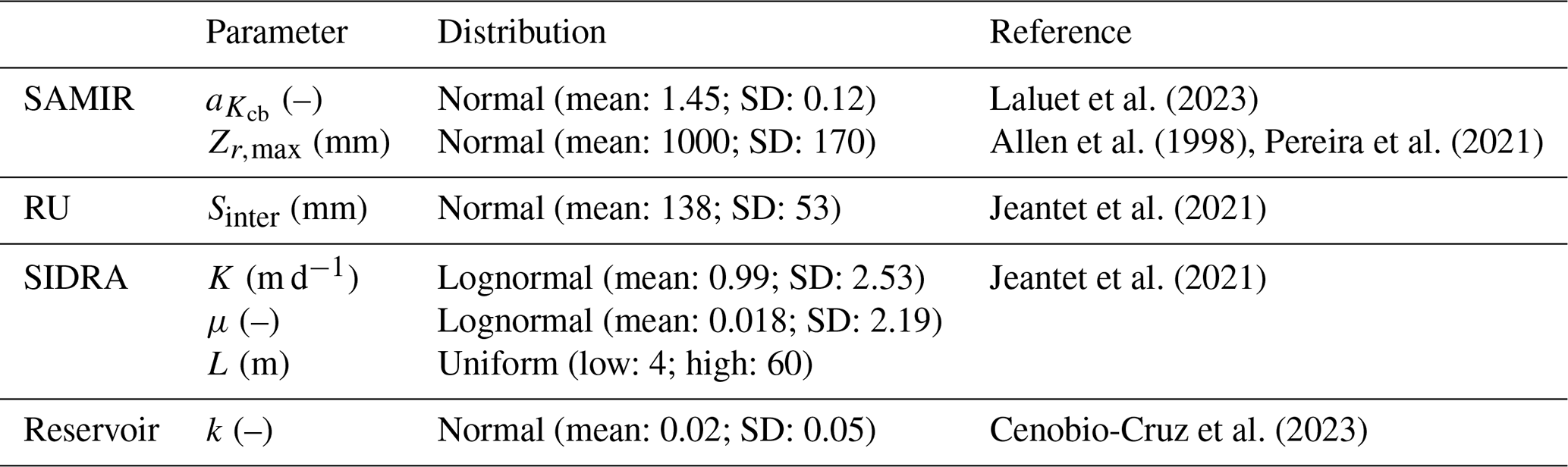
2.3.2 Parameter distribution for calibration

NSGA-II requires a distribution provided by the user for each calibrated parameter. The distribution and references used in this study are provided in Table 3.

The distribution of $a_{K_{\mathrm{cb}}}$ of the SAMIR model is based on Laluet et al. (2023a), who obtained $a_{K_{\mathrm{cb}}}$ values for 37 agricultural seasons (mainly maize and wheat, being widely present in the AB district) from the linear relationship K_cb $=a_{K_{\mathrm{cb}}}\cdot$ NDVI $+b_{K_{\mathrm{cb}}}$. Knowing the value of NDVI in bare soil (where K_cb is zero) and at full vegetation (where K_cb is equal to K_cb,max), $a_{K_{\mathrm{cb}}}$ and $b_{K_{\mathrm{cb}}}$ can be inferred.

The distribution of Z_r,max is derived from tables provided by Allen et al. (1998) and Pereira et al. (2021). This study uses the mean and standard deviation of Z_r,max for maize, being the most present and irrigated crop type at AB1 and AB2.

The distribution of S_inter of the RU model is taken from Jeantet et al. (2021), who calibrated this parameter based on drainage discharge in situ data from 22 drained French sites.

The distribution of K and μ of the SIDRA model is also based on Jeantet et al. (2021), who derived the mean and standard deviation of these parameters from field measurements performed on 15 silty soils in France, with similar soil textures to those of AB1 and AB2. Half of the drain spacing parameter L distribution was chosen to be wide (uniform distribution between 4 and 60 m), taking into consideration that some plots are not drained at AB1 and AB2. As a comparison, Chelil et al. (2022) used a uniform distribution between 3.5 and 6 m for fully drained sites.

The distribution of the ω parameter of the Reservoir model is derived from Cenobio-Cruz et al. (2023), who calibrated this parameter based on discharge flow data of about 25 catchments in northern Spain.

2.3.3 Metrics used for calibration and validation

For drainage calibration, the Kling–Gupta efficiency (KGE) (Gupta et al., 2009) is used:

$$\begin{array}{}\text{(14)}& \mathrm{KGE}=\mathrm{1}-\sqrt{{\left(r-\mathrm{1}\right)}^{\mathrm{2}}+{\left(\mathit{\alpha }-\mathrm{1}\right)}^{\mathrm{2}}+{\left(\mathit{\delta }-\mathrm{1}\right)}^{\mathrm{2}}},\end{array}$$

where r is the Pearson's correlation coefficient, α is the bias component, and δ is the ratio of the discharge variance.

$$\begin{array}{}\text{(15)}& \mathit{\alpha }={\displaystyle \frac{m_{\mathrm{s}}}{m_{\mathrm{o}}}}\mathrm{and}\mathit{\delta }={\displaystyle \frac{{\mathit{\sigma }}_s}{{\mathit{\sigma }}_o}}\end{array}$$

In the above, m and σ are the mean and standard deviation, respectively. Subscripts s and o represent the simulated and observed flow, respectively.

Since the KGE tends to place more weight on high flows (Santos et al., 2018), we used KGE (Q^0.5). KGE (Q^0.5) is the KGE calculated from the square roots of simulated and observed drainage, allowing the weights between high and low flows to be more balanced. Following Jeantet et al. (2021), we consider simulations to be “excellent” when KGE (Q^0.5) is larger than 0.8, “very good” when it is larger than 0.7, “good” when it is larger than 0.6, “acceptable” when it is between 0.5 and 0.6, and “unsatisfactory” when it is below 0.5. Furthermore, to get a reference in mind, a KGE of −0.41 is equivalent to having a simulation performance equal to the average of the observed data (Knoben et al., 2019).

The RMSD objective function is used for irrigation calibration:

$$\begin{array}{}\text{(16)}& \mathrm{RMSD}=\sqrt{{\displaystyle \frac{{\sum }_{i=\mathrm{1}}^j({\widehat{y}}_i-y_i{)}^{\mathrm{2}}}{j}}},\end{array}$$

where j is the number of days in the simulated time series, i is 1 d of the time series, ${\widehat{y}}_i$ is the simulated time series, and y_i is the reference time series. We consider irrigation to be well simulated when the RMSD calculated between the irrigation measured at the pumping station and the one simulated by SAMIR for all the plots in AB is below 0.70 mm d⁻¹. This value corresponds to the average RMSD found from 2017 to 2021 by Olivera-Guerra et al. (2023).

2.4 Strategy for evaluating the models' accuracy

Complementarily to the evaluation of the models' precision, this study also aims to assess the accuracy of the four models. We remind the readers that, by accuracy, we mean the ability of a model to approximate the observed data as closely as possible by relying only on default values given by the literature for its main parameters, i.e., without any site-specific calibration step.

To this end, for each of the four models, 2000 sets of their most sensitive parameters are generated randomly using a Monte Carlo sampling with the distributions presented in Table 3, except for half of the drain spacing L. Indeed, for the accuracy evaluation, we consider a situation where we have no information on the geometry of the drainage network and therefore on L. In this hypothetical situation, we do not know if a portion of the surface is not drained, potentially resulting in high L values. Therefore, we use a value of 6 m for the accuracy evaluation, which is a value frequently found in the literature (Jeantet et al., 2021). In addition, to focus only on the drainage accuracy evaluation, the irrigation obtained with SAMIR during the precision evaluation step is injected into SAMIR as a forcing. The KGE (Q^0.5) obtained with a simulation performed with average default parameters is calculated, and the ensemble generated by the 2000 Monte Carlo simulations is analyzed.

Table 3 Distributions of the main parameters calibrated with the NSGA-II algorithm to evaluate the models' precision and associated references.

2.5 Complexity of models' calibration

The models involving SAMIR are more complex to calibrate than those involving RU. This is due, in particular, to the fact that (i) SAMIR-based models involve input data that are not always readily available at the required fine resolution (in particular, land use maps), and (ii) SAMIR is spatialized and therefore requires more computing resources (several hours of computation for 2000 simulations based on the AB district with 8 GB RAM and four CPUs running in parallel). The RU-based models are simpler to calibrate than the SAMIR-based ones because RU requires only meteorological data as input, and they are not spatialized and demand fewer computing resources (a few minutes to run 2000 simulations on the AB district with the same computing configuration).

The two subsurface models are simple and require few computing resources. SIDRA-based models are slightly more complex to calibrate than Reservoir-based models as they require two drainage network characteristic parameters (half of the drain spacing and depth of drains) as input. However, they are not the most sensitive parameters in the SIDRA model (Henine et al., 2022; Chelil et al., 2022).

We see a gradient in terms of the level of complexity and expertise required to calibrate the models, namely from SAMIR-SIDRA to RU-Reservoir. The four models are coded in Python, as is the NSGA-II calibration algorithm provided by the Python package spotpy.

3 Results and discussion

3.1 Precision evaluation

This section will first give a quick overview of the irrigation simulated by SAMIR and used as a forcing by RU. The precision of the drainage simulated by each model is then presented. Finally, we will explain why the model precision differs between the four models, and we will provide some recommendations and perspectives.

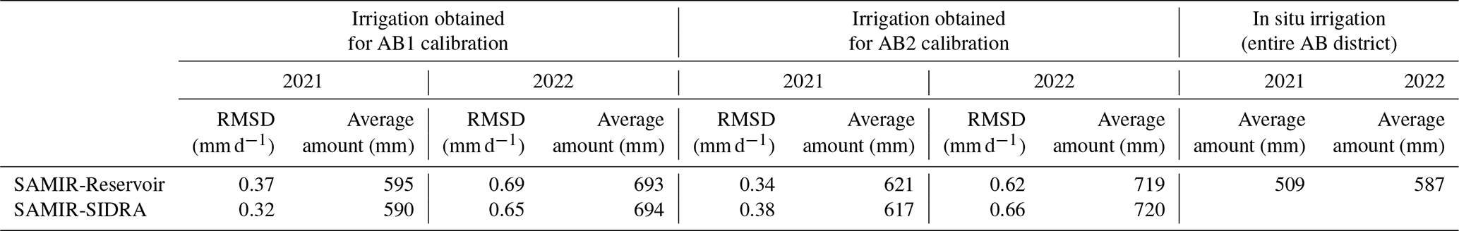
3.1.1 Irrigation simulated by SAMIR

Table 4 shows, for SAMIR-Reservoir and SAMIR-SIDRA, the RMSD obtained between the simulated and observed irrigation at the pumping station over all the irrigated plots of AB resulting from the NSGA-II multi-objective calibration performed for AB1 and AB2. The average RMSD obtained is 0.35 mm d⁻¹ for 2021 and 0.66 mm d⁻¹ for 2022, in line with the quality criteria defined previously (< 0.70 mm d⁻¹). The average amount of irrigation simulated for the AB1 sub-basin is 592 mm for the period from May to October 2021 and 693 mm for the period from May to October 2022. For AB2, it is 619 mm in 2021 and 720 mm in 2022. These amounts are fully consistent given the amounts of irrigation measured at the pumping station and the proportions of surface used for double crops and summer cereals in each AB1 and AB2 sub-basin compared to those in the entire AB district (see Table 2).

Table 4 RMSD between daily simulated and observed irrigation, seasonal (between May and October for each year) cumulated simulated irrigation obtained with site-calibrated SAMIR-Reservoir and site-calibrated SAMIR-SIDRA separately, and seasonal in situ irrigation over the whole AB district (including non-irrigated plots).

3.1.2 Which model is more precise?

Figures 4 and 5 compare the simulated and observed drainage for the AB1 and AB2 sub-basins, respectively, and for the 2021 and 2022 periods. Table 5 shows that, among the 16 combinations of model–sub-basin–period, nine have KGE (Q^0.5) values considered to be excellent, four are very good, two are good, and one is acceptable; there is no unsatisfactory simulation. RU-Reservoir stands out as the most precise model (mean KGE (Q^0.5) = 0.87), followed by SAMIR-Reservoir (0.79), RU-SIDRA (0.76), and SAMIR-SIDRA (0.68). From these results, two highlights stand out:

• i.

  The models based on Reservoir are more precise in terms of drainage simulations than those based on SIDRA. This is particularly true for the AB1 sub-basin.

• ii.

  The models based on RU are more precise in terms of drainage simulations than those based on SAMIR.

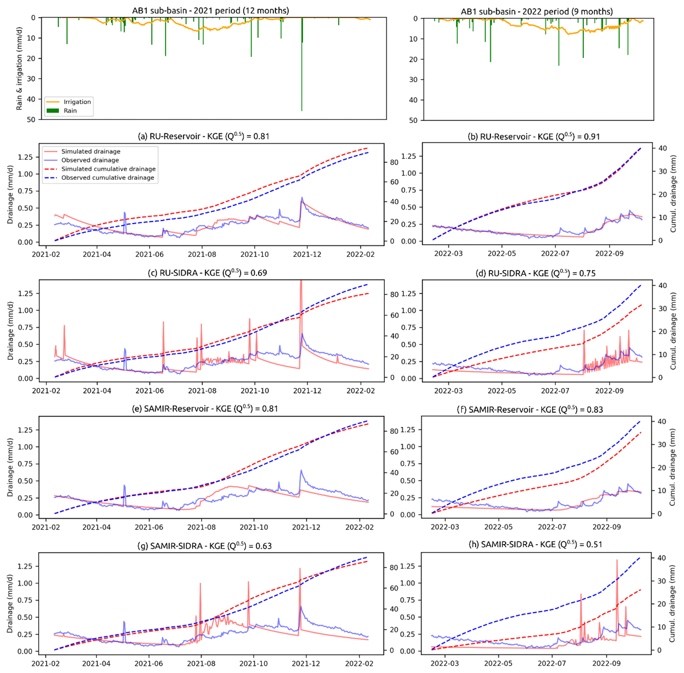
Figure 4 Daily and cumulated drainage of the AB1 sub-basin simulated by the four site-calibrated models for 2021 (left) and 2022 (right) periods. Plots at the top show the observed precipitation and the simulated irrigation.

Figure 5 Same as Fig. 4 but for AB2 sub-basin.

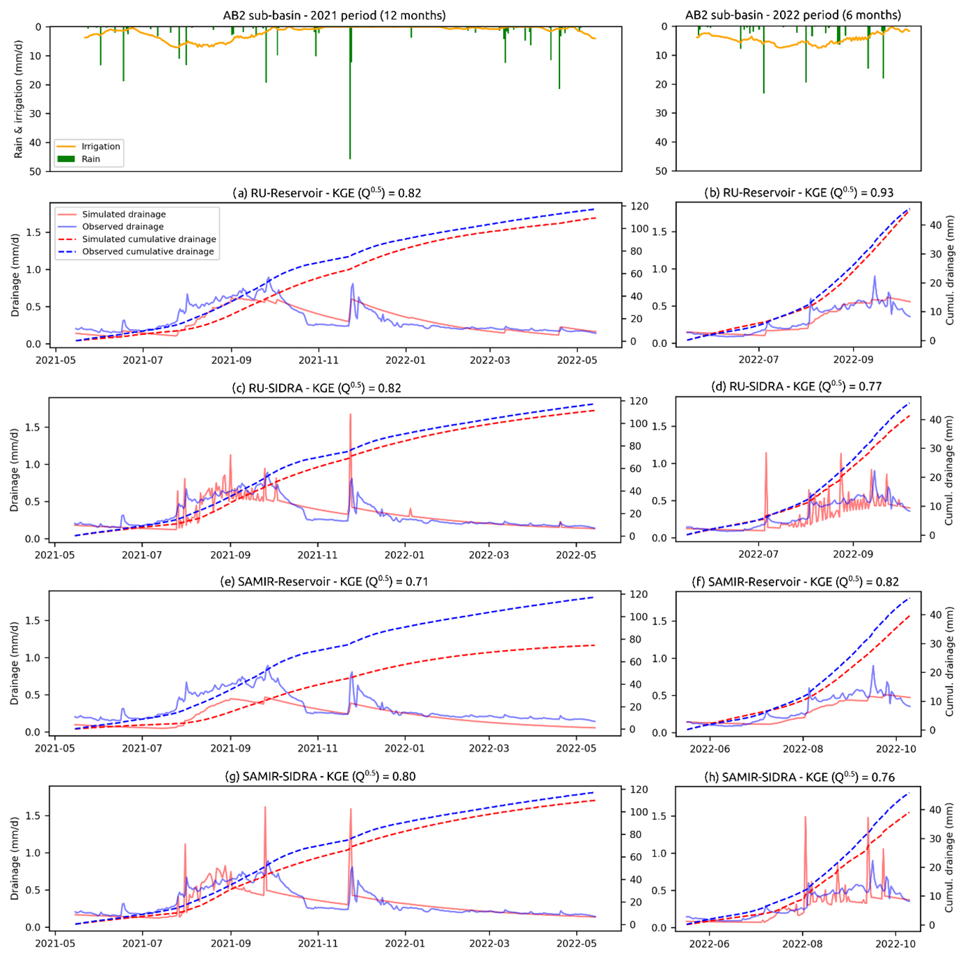
Table 5 KGE (Q^0.5) obtained with NSGA-II calibration for the AB1 and AB2 sub-basins, the four models, and both study periods. Values above 0.8 are considered to be excellent, values between 0.7 and 0.8 are considered to be very good, values between 0.6 and 0.7 are considered to be good, and values between 0.5 and 0.6 are considered to be acceptable.

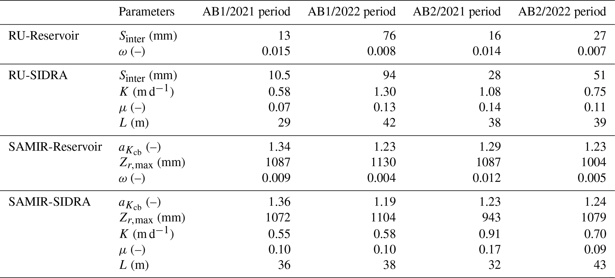
Table 6 Parameter values obtained with NSGA-II calibration for the AB1 and AB2 sub-basins, the four models, and both study periods.

3.1.3 Why are Reservoir-based models more precise?

The differences in the formalism of Reservoir and SIDRA and the low responsiveness of the AB1 and AB2 hydrosystems explain the better performance of the site-calibrated RU-Reservoir and SAMIR-Reservoir models. Indeed, SIDRA was designed to simulate flow peaks followed by relatively steep recession curves. In contrast, Reservoir does not simulate peaks and generates flow according to a depletion coefficient ω that can be very low. However, the measured drainage dynamics for AB1 and AB2 are representative of hydrosystems showing low responsiveness. This can be seen in Figs. 4 and 5, where the 40 mm rainfall in December 2021 generates a peak of less than 1 mm d⁻¹ for both sub-basins, followed by a smooth recession curve with a discharge that never reaches 0 during the hydrological year. In comparison, the data used by Jeantet et al. (2021) from 22 French experimental sites, accounting for nearly 200 hydrological years, show winter peaks exceeding 20 mm d⁻¹ in most of the studied years, followed by steep recession curves where 0 flow is reached in a few weeks. Therefore, the Reservoir model is favored by the low responsiveness of the AB1 and AB2 hydrosystems, especially for AB1. The SIDRA model shows a better precision for AB2 than AB1 because AB2 is more responsive, with larger amounts of discharge. In addition, the values of the Reservoir depletion coefficient ω are low at our sites (0.009 on average) compared to those obtained by Cenobio-Cruz et al. (2023) (0.02 on average), which again reflects the relatively low responsiveness of the studied area.

The soil does not explain this low responsiveness since the mean calibrated values of K and μ (0.81 m d⁻¹ and 0.11 m³ m⁻³, respectively; see Table 6) are consistent with the order of magnitude found in Jeantet et al. (2021) for a similar soil type (K from 0.1 to 1.8 m d⁻¹ and μ from 0.05 to 0.08 m³ m⁻³). The explanation seems to lie in the fact that the surfaces of AB1 and AB2 are not fully equipped with field drains. The transfer time from the recharge location to the main drain would be longer on non-equipped plots. The values of the calibrated half of the drain spacing L support this assumption, with an average of 37 m (see Table 6), being a value that could represent an average between low L values for plots equipped with field drains and high L values for plots that are not equipped with field drains.

3.1.4 Why are RU-based models more precise?

To understand the better performance of the site-calibrated RU-Reservoir and RU-SIDRA models in comparison with SAMIR-Reservoir and SAMIR-SIDRA, respectively, it is again necessary to look at the differences in formalism between RU and SAMIR. Indeed, RU, unlike SAMIR, has a stage during which a reduction factor β of 0.33 is applied to the recharge (Eq. 8; this stage is triggered by the water level in the soil reservoir). In AB1 and AB2, this stage is triggered particularly during the irrigation season and results in the spread of recharge amounts. This benefits RU-SIDRA, which, owing to the lower recharge events simulated by RU, generates lower peaks, consistent with the drainage observations. This process is well illustrated in Fig. 4d, where RU-SIDRA simulates numerous small peaks during the irrigation period, allowing better matching of the observations. In contrast, in Fig. 4h, SAMIR-SIDRA simulates larger and fewer peaks.

Furthermore, the S_inter values of RU obtained through calibration are very low (17 mm on average for the 2021 period and 61 mm for the 2022 period; see Table 5) compared with those obtained by Jeantet et al. (2021) (138 mm on average). This is because the RU-based models are not spatialized and use average irrigation derived from the irrigation simulated by SAMIR, whether for intensely irrigated corn plots generating a lot of recharge or for non-irrigated plots generating no recharge. RU-based models simulate less recharge by simulating an average plot using average irrigation. To compensate for this, the NSGA-II optimization algorithm finds low S_inter values to reduce the reservoir size and, therefore, the ET, which in turn increases the recharge. This explains the low S_inter values retrieved over AB1 and AB2.

3.1.5 Variability of calibrated parameter values between the two periods analyzed

We can see from Table 6 that the calibrated values of most parameters vary between the two periods for a given sub-basin. These variations indicate a lack of predictive capacity of the models, at least between the two periods analyzed (using the parameter values obtained from calibration based on the first period, the models fail to predict the second period). We believe this is due to the semi-empirical nature of the models. Indeed, parameter values vary between the two periods to compensate for the fact that physical processes (e.g., lateral subsurface flows, root growth, evapotranspiration) are either too empirically simulated or neglected.

3.1.6 Recommendations and perspectives

Based on the results obtained over AB by the four models with varying complexity levels, we recommend using RU-Reservoir when drainage data are available for calibration. The simplest model can reproduce the drainage observed at the AB1 and AB2 outlets fairly well. The RU-Reservoir model efficiently combines the performance of RU (allowing a better temporal distribution of recharge than SAMIR) and Reservoir (offering drainage simulations with relatively low responsive dynamics), which fits perfectly with the present study. However, if a study concerns a more responsive hydrosystem with larger peaks and steeper recession curves, we recommend using RU-SIDRA. Indeed, for the AB2 sub-basin, which is slightly more responsive than AB1, RU-SIDRA shows, during the 2021 period (Fig. 5c), a precision comparable to that of RU-Reservoir (Fig. 5a). This leads us to assume that RU-SIDRA could be more appropriate than RU-Reservoir for even more responsive hydrosystems.

To support the strength of these recommendations and to ensure that the models can be ultimately used as decision support tools with confidence, we believe it is necessary to improve the robustness of the models by better simulating certain physical processes (e.g., lateral subsurface flows, root growth, evapotranspiration). Indeed, the variability of calibrated parameter values between the two periods indicates their limited robustness.

Since RU is not spatialized and has a very simple formalism, the models based on it are more straightforward to run and require fewer resources than those based on SAMIR. However, they do not consider the spatial heterogeneity in irrigation generally encountered in irrigated sub-basins, resulting in calibrated Sinter values that are too low to simulate enough recharge. Spatialization of the RU-based models with irrigation data for each plot would lead to higher calibrated S_inter values that are more consistent with those proposed in Jeantet et al. (2021). However, unlike SAMIR, RU cannot simulate irrigation, and its spatialization would require plot-scale irrigation data that are rarely available.

In some cases, SAMIR shows a relatively low KGE (Q^0.5) and difficulties reproducing the right amount of drainage (see Figs. 4d, h, and 5e). Modifying the SAMIR formalism by taking inspiration from RU and adding a stage related to the soil water availability in which recharge is limited by a factor β could help improve the precision of SAMIR-SIDRA and SAMIR-Reservoir.

3.2 Accuracy evaluation

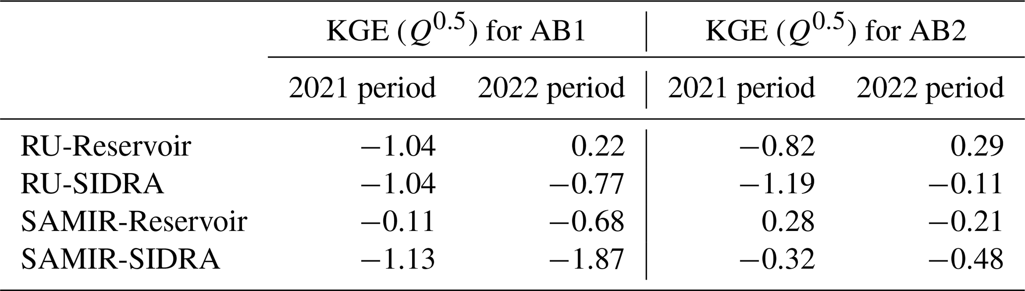
Figures 6 and 7 show, for each of the 16 model–sub-basin–period combinations, the drainage simulated by using the mean values of the default parameters as input (red line) and the 2000 model runs from randomly generated input parameter sets within pre-defined distributions provided by the literature (gray lines). Table 7 summarizes the KGE (Q^0.5) obtained with the average default parameters. It indicates that all 16 cases present unsatisfactory KGE (Q^0.5) values (below 0.5). Moreover, nine cases show KGE (Q^0.5) values lower than −0.41, the value corresponding to the KGE obtained with the temporal average of the observed data.

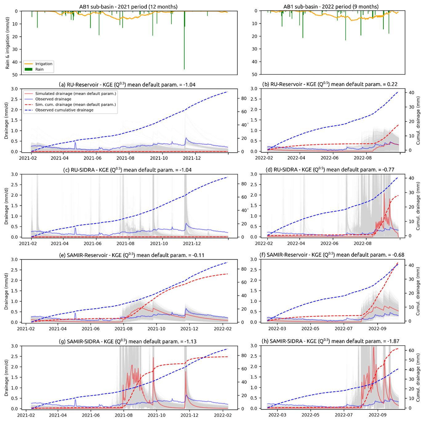
Figure 6 Daily drainage of the AB1 sub-basin simulated using average default parameters of the four models separately (red line) and the drainage value ensemble obtained by running each model 2000 times using randomly generated input parameter sets within pre-defined distributions (gray lines).

Figure 7 Same as Fig. 6 but for the AB2 sub-basin.

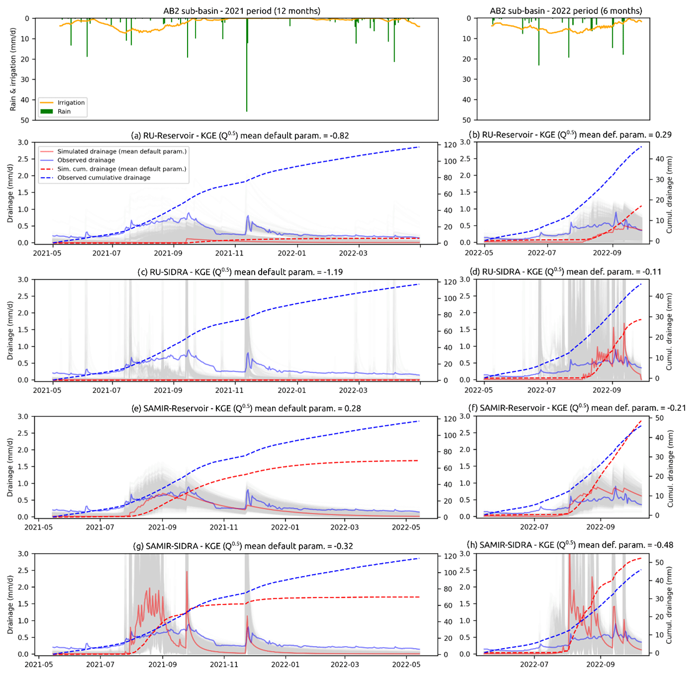
RU-Reservoir shows relatively satisfactory KGE (Q^0.5) for 2022 (0.22 for AB1 and 0.29 for AB2). However, when looking at the drainage dynamics and amounts illustrated in Figs. 6b and 7b, it appears that these performances are due to the nature of the objective function KGE (Q^0.5), giving significant importance to low flows. SAMIR-Reservoir shows a relatively good KGE (Q^0.5) for AB2 for 2022 (0.29). Furthermore, the timing and quantities that SAMIR-Reservoir simulated for AB1 for both periods of 2021 and 2022, as well as for AB2 for the 2021 period, are more consistent than those simulated by the other three models.

Table 7 KGE (Q^0.5) values obtained with average default values of model parameters for the AB1 and AB2 sub-basins, the four models, and the two study periods separately.

3.2.1 Accuracy of RU-Reservoir and RU-SIDRA

Figures 6a and c and 7a and c show that the RU-based models do not simulate any discharge for the 2021 period with the average default parameters (red lines). This is related to the fact that, in a context where RU is not spatialized while irrigation is spatially heterogeneous, the optimal S_inter value to generate sufficient recharge is lower than in the literature (optimal S_inter values are shown in Table 5). The S_inter values taken from the literature for the accuracy evaluation are then too high to simulate enough recharge. This implies that, without calibration with drainage data, models based on RU are only effective in contexts where irrigation practices are homogeneous, e.g., on sites under monoculture. Note that, for the 2022 period, the RU-based models simulate more drainage than in 2021 because the irrigation amounts applied by farmers in 2022 (587 mm between May and October 2022, on average, over the AB district) are significantly larger than in 2021 (509 mm between May and October 2021).

3.2.2 Accuracy of SAMIR-SIDRA

Figures 6 and 7 show that, with average default parameter values, the SAMIR-based models simulate the drainage dynamics with some consistency with the irrigation season and the rain events for both the 2021 and 2022 periods. However, SAMIR-SIDRA shows lower performance than SAMIR-Reservoir. Several factors may explain this result. First, although they are physical parameters, the values of the SIDRA parameters K and μ found in the literature do not necessarily correspond to their optimal values for a given site. Second, SIDRA is more appropriate for more responsive hydrosystems than AB1 and AB2. Finally, the lack of information regarding half of the drain spacing L in the AB district led us to set it at 6 m, whereas, when calibrated based on AB1 and AB2, this parameter is, on average, 37 m (average value considering the plots that are not equipped with field drains). This lower L value results in a high reactivity in terms of the simulated drainage.

3.2.3 Accuracy of SAMIR-Reservoir

Figures 6e and f and 7e and f show that the drainage simulated by SAMIR-Reservoir with average default parameter values is more consistent with the observed drainage than the other three models. It also presents less variability within the ensemble of 2000 simulations. Figure 7e shows that SAMIR-Reservoir simulates the drainage dynamics and quantities particularly well for the AB2 sub-basin during the 2021 period. SAMIR-Reservoir tends to overestimate the drainage when the discharge is lower for AB1 during the 2021 and 2022 periods and for AB2 during the 2022 periods. The fact that SAMIR-Reservoir shows higher accuracy than the more complex models using SIDRA is an interesting result since it shows that the descriptive complexity of the models may not be useful for predictive purposes. One reason for this is the difficulty of linking SIDRA soil parameters to physically measurable soil properties.

The SAMIR-Reservoir accuracy varies spatially between AB1 and AB2 and temporally between 2021 and 2022. These differences reflect the semi-empirical nature of the SAMIR and Reservoir models. Indeed, they can be attributed to the impact of unrepresented processes (e.g., lateral flows) or the misrepresentation of ET and recharge processes in unusual situations (e.g., 2022 drought and heatwaves). SAMIR, especially, fully neglects the lateral flow. Such subsurface flows may come from outside sub-basin boundaries and contribute significantly to the sub-basin discharge measured at the outlet, depending on the hydrometeorological conditions encountered in a given year. Note that representing subsurface lateral flows would be challenging, especially to estimate them accurately across system boundaries. Furthermore, this would require more complex models than those tested in this study, as well as additional data (e.g., piezometric), which are currently not available in the study area.

3.2.4 Recommendations and perspectives

Due to the semi-empirical nature of the four models investigated in this study, it is difficult to reproduce the drainage discharge with default parameters from the literature. A limitation of RU-based models is their lack of spatialization, leading to the use of an average irrigation in forcing, while the irrigation of AB1 and AB2 sub-basins is spatially heterogeneous. This results in RU not having enough irrigation to generate a correct recharge with the S_inter values suggested in the literature (being too high). One way to overcome this would be to spatialize RU with irrigation data at each plot, but these data are rarely available.

SAMIR-Reservoir offers a certain consistency with the observed data and could provide an approximate idea of the drainage dynamics and amounts occurring in an ungauged irrigated sub-catchment. Figures 6e and f and 7e and f show that the 2000 simulations obtained with SAMIR-Reservoir are less dispersed than for the other three models, suggesting a greater robustness. For decision support, we therefore recommend the use of SAMIR-Reservoir. However, its accuracy should be further evaluated based on other sites and could be improved (i) by modeling lacking physical processes and (ii) by investigating a link between the depletion coefficient parameter ω and the soil texture or the characteristics of the drainage network.

4 Summary and conclusion

Estimating the drainage in semi-arid irrigation conditions is essential to prevent soil salinization issues and to assess the water productivity and the irrigation impact on downstream ecosystems. A few studies have used physically based models to simulate drainage in an irrigated context. However, these models have many parameters requiring extensive data that are rarely available. In this paper, we thus assessed the capacity of four parsimonious semi-empirical models to simulate drainage at the scale of two sub-basins of the AB district in northeastern Spain. The four models are built from the combination of two surface models (RU and SAMIR) and two subsurface models (Reservoir and SIDRA) with varying complexity levels: RU-Reservoir (two main parameters), RU-SIDRA (three main parameters), SAMIR-Reservoir (three main parameters), and SAMIR-SIDRA (four main parameters). SAMIR is based on the FAO-56 ET and crop water balance formulations relying on two main sensitive parameters, while RU is a simplified version of the FAO-56, relying on a single sensitive parameter only. SIDRA solves the Boussinesq equation from two main sensitive parameters, while Reservoir is an empirical drainage model based only on a single depletion parameter.

The precision of the four models, i.e., their ability to reproduce observed drainage data with a site-specific calibration, was first evaluated. An optimal calibration approach was implemented for each model and each sub-basin using the multi-objective genetic algorithm NSGA-II. The comparison between the drainage simulated by site-specific calibrated models and observations indicates that RU-Reservoir presents a better precision, followed closely by SAMIR-Reservoir. This is explained by the fact that the Reservoir model is well suited to representing the low responsiveness of both studied sub-basins and that the RU model manages better in artificially spreading out the recharge events during the irrigation period than the SAMIR model. In addition, the calibrated parameter values vary between the two periods analyzed for a given sub-basin. This indicates that the models have limited predictive capacities (robustness). It is therefore necessary to identify the processes that are poorly simulated or not simulated at all, such as lateral subsurface flows, root growth, and evapotranspiration, and to better take them into account in the models.

Complex models, with many processes being simulated and many parameters to calibrate, are likely to simulate drainage more precisely than simple models when calibrated based on observed data. However, when no data are available for calibration, the most complex models are also the most prone to uncertainty (Puy et al., 2022). Moreover, drainage observations required for site-specific calibration are rarely available. Therefore, the accuracy of the four models was also evaluated. By accuracy, we mean the ability of the four models to reproduce the observed drainage using default parameter values provided by the literature. The comparison between the drainage simulated by default-calibrated models and observations indicates that SAMIR-Reservoir is the only model among the four tested that is capable of giving a rough estimate of the drainage dynamics and amounts from default parameters.

However, it was found that the accuracy of SAMIR-Reservoir is quite variable from one sub-basin to another and from one hydrological year to another. Therefore, calibration strategies are still needed to reduce uncertainties in SAMIR-Reservoir drainage estimates in sub-basins with contrasting conditions. In addition, better constraining the value of the Reservoir's depletion coefficient ω, especially by seeking a link with soil texture or with the characteristics of the drainage network, should be investigated in future studies to improve the accuracy of SAMIR-Reservoir.

Furthermore, our study took place in an irrigation district where the water use is known and accurately monitored through the pumping data. Such irrigation data are rarely available in practice, and no model can predict drainage accurately based on inaccurate irrigation forcing, regardless of the model calibration issue. Hence, it is crucial to develop tools to retrieve the irrigation practices, notably at the integrated spatial scales of sub-basin or irrigation districts. To this end, many recent works seek to assimilate satellite products of soil moisture or ET in crop water balance models at a range of scales (e.g., Ouaadi et al., 2021; Massari et al., 2021; Dari et al., 2023; Olivera-Guerra et al., 2020). The coupling of such remote sensing approaches with surface and subsurface models is likely to improve the predictive capabilities of drainage in irrigated areas.