Regionalization of GR4J model parameters for river flow prediction in Paraná, Brazil

Regionalization methods dependent on hydrological models comprise techniques for transferring calibrated parameters in instrumented watersheds (donor basins) to non-instrumented watersheds (target basins). There is a lack of flow regionalization studies in regions with humid subtropical and hot temperate climates, and one of the main novelties of this research is to assess the regionalization of low flows in Paraná in the south of Brazil. In addition to filling this gap, this research presents innovative artificial-intelligence techniques for transferring parameters from hydrological models. This study aims to evaluate regionalization methods for transferring GR4J parameters and predicting river flow in catchments from the south of Brazil. We created a dataset for the state of Paraná with daily hydrological time series (precipitation, evapotranspiration, and river flow) and watershed physiographic and climatological indices for 126 catchments. Rigorous quality-controlling techniques were applied to recover data from 1979 to 2020. The regionalization methods compared in this study are based on simple spatial proximity, physiographic–climatic similarity, and regression by random forest techniques. Direct regression of Q₉₅ was calculated using random forest techniques and compared with indirect methods, i.e. using regionalization of GR4J parameters. A set of 100 basins was used to train the regionalization models, and another 26 catchments (pseudo-non-instrumented) were used to evaluate and compare the performance of regionalizations. The GR4J model showed acceptable performances for the sample of 126 catchments, with 65 % of watersheds presenting a log-transformed Nash–Sutcliffe coefficient greater than 0.70 during the validation period. According to the evaluation carried out for the sample of 26 basins, regionalization based on physiographic–climatic similarity was shown to be the most robust method for the prediction of daily and Q₉₅ reference flow in basins from the state of Paraná. When increasing the number of donor basins, the method based on spatial proximity has comparable performance to the method based on physiographic–climatic similarity. Based on the physiographic–climatic characteristics of the basins, it was possible to classify six distinct groups of watersheds in Paraná. Each group shows similarities in forest cover, urban area, number of days with more than 150 mm of precipitation, and average duration of consecutive dry days. Although the physiographic–climatic similarity method obtained the best performance, the use of machine learning algorithms to regionalize the model parameters had good performance using climatic and physiographic indices as inputs. This research represents a proof of concept that basins without flow monitoring can have a good approximation of streamflow if physiographic–climatic information is provided.

1 Introduction

According to Razavi and Coulibaly (2013), regionalization methods dependent on rainfall–runoff models comprise techniques for transferring calibrated parameters in instrumented basins (donor basins) to non-instrumented basins (target basins). The study carried out by Arsenault et al. (2019) presents three techniques based on physical similarity, spatial proximity, and regression to estimate the parameters of three different hydrological models, with the purpose of predicting flows in watersheds that do not have monitoring. Although many advances have been made in this area of hydrology, there are still uncertainties in methods for estimating flows in ungauged basins (Guo et al., 2020). Part of this is due to the uniqueness of each region across the globe, which concerns not only the uniqueness of each location but also the issue of availability of information (e.g. descriptive characteristics of basins and availability of hydrometeorological data). Additionally, hydrological systems are dependent on temporal and spatial scales with interactions between climate, vegetation, topography, and soil (Blöschl et al., 2013; Hrachowitz et al., 2013) that make the task of estimating hydrological information in basins with little or no data challenging.

The watersheds analysed in this research belong to the southern region of Brazil, with an area of approximately 199 315 km². The hydrography of Paraná is composed mainly of the Iguazu River, Paraná River, Paranapanema River, Tibagi River, Ivaí River, and Piquiri River. The study of low flows and droughts is critical in the context of water availability in Brazil; river dams and reservoirs are used for power generation (70 % of Brazilian energy sector), to provide drinking water for the population, to irrigate crops, and to distribute water for industrial use (Carneiro et al., 2020). The Paraná basin, a major hydroelectricity-producing region with 32 % (60 million people) of Brazil's population, experienced very severe drought in 2000 and 2014, compromising the water supply for 11 million people in São Paulo (Melo et al., 2016). The state of Paraná faced one of the worst droughts in its history between 2020 and 2021 (Cunha et al., 2019; Juliani et al., 2020). There are few studies of flow regionalization in the south of Brazil (Kaviski et al., 2002; Bazzo and Almeida, 2016); at the same time, the hydrological measurements and field work in the area are declining (Burt and McDonnell, 2015; Melo et al., 2020). Our work brings novel contributions for watersheds with similar climate and geography; also, it provides more information for governmental planning and management.

In order to reveal research gaps and how our study goes beyond the existing literature, we highlight the following points: (i) the need to better understand regionalization techniques in a subtropical climate, which has very distinct and specific runoff generation mechanisms; (ii) a proof of concept that basins without flow monitoring can have a good approximation of streamflow if other physiographic–climatic indices are provided; and (iii) the fact that machine learning algorithms perform better with physiographic–climatic indices as inputs.

The aim of this article is to improve the methodology for transferring parameters of the GR4J model calibrated in instrumented watersheds to predict daily flows in basins with little or no hydrological information. The performance of different regionalization methods are verified in Paraná basins that have a history of hydrometeorological data records. Other objectives are the following: (i) build a hydrological database for the state of Paraná, Brazil (the database consists of daily flow, precipitation, and evapotranspiration time series and catchment-related descriptive indices); (ii) develop and improve methods for transferring GR4J calibrated parameters through regionalization techniques based on spatial distance, physiographic–climatic similarity, and non-linear regression; and (iii) compare regionalization methods and random forest techniques to estimate the Q₉₅ reference flow.

2 Data for state of Paraná

The study area was delimited based on the hydrographic network of the state of Paraná, Brazil, which is available at Instituto Água e Terra (IAT) (IAT, 2020), and on a rectangular polygon demarcated between latitudes of 22°15^′36^′′ and 26°54^′00^′′ S and longitudes of 48°00^′00^′′ and 54°42^′00^′′ W. Therefore, the study area includes the state of Paraná and extends into parts of the states of Santa Catarina and São Paulo, not completely covering the Paranapanema and Paraná river basins (Fig. 1).

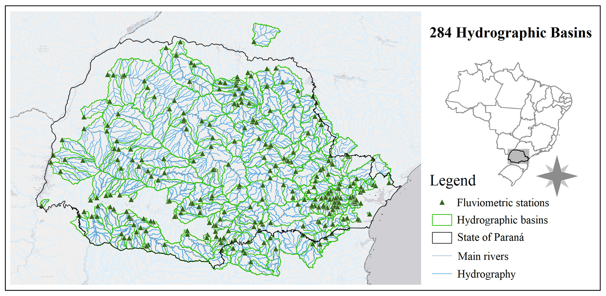
Figure 1 River flow stations and watershed delineation.

Time series of hydrometeorological observations were obtained at Agência Nacional de Águas e Saneamento Básico (ANA) via HidroWEB Portal, Instituto Nacional de Meteorologia (INMET), Sistema de Tecnologia e Monitoramento Ambiental do Paraná (Simepar), Água e Terra Institute (IAT), and Instituto de Desenvolvimento Rural do Paraná (IAPAR-EMATER).

Although there are datasets at a national level, such as CAMELS-BR (Chagas et al., 2020) and CABra (Almagro et al., 2021), the authors decided to construct a new dataset based on the hydrographic network of the state of Paraná. This network has a consistent topology and codification; its hierarchization was proposed by Otto Pfafstetter (Pfafstetter, 1989) and allows the extraction of information upstream and downstream of each river section (Sousa et al., 2009).

2.1 Precipitation time series

The Llabrés-Brustenga et al. (2019) quality control method was used to evaluate daily rainfall data series from 1389 stations, which are shown in Fig. 2. The method can be divided into four steps. First, stations coordinates, the period of operation, and the percentage of available data are checked. In the second stage, data that are not physically possible are identified and discarded, such as negative precipitation values and extreme events greater than 300 mm.

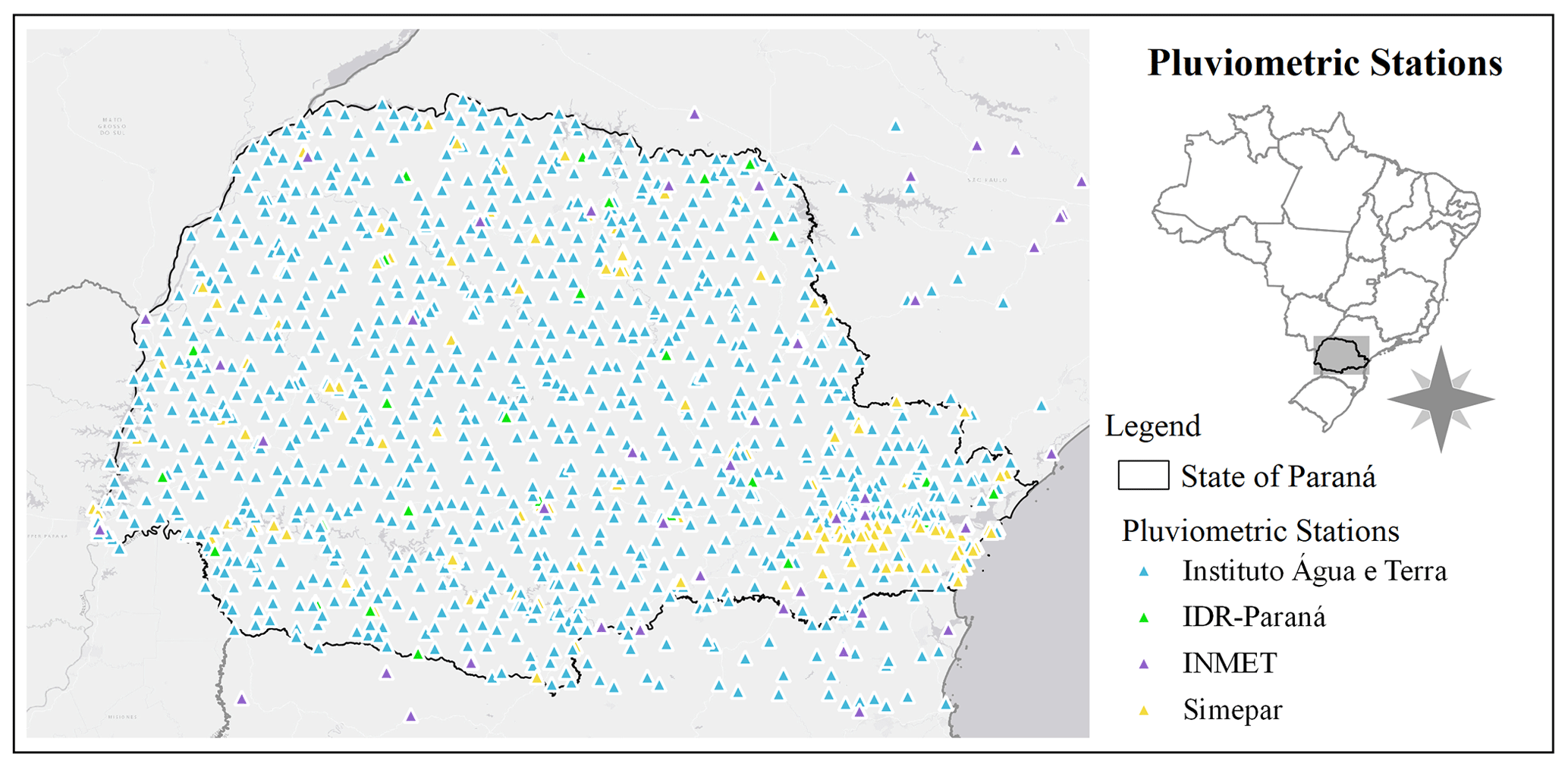
Figure 2 Location of pluviometric stations.

The third stage consists of analysing the historical series of each station individually. For each year, a quality index is calculated, which depends on five factors, namely (i) the percentage of data available in each year of the series; (ii) the distribution of failures throughout the year, for which the penalty becomes greater for a series that has long continuous periods of failures; (iii) the probability that the series is formed by possible failures that have been padded with zeros, which penalizes the series that have monthly cumulative data equal to zero, indicating that “false zeros” are possible; (iv) the probability of systematic accumulation of two or more days of the week, which penalizes the station if a day of the week with a tendency for less rain than other days of the week is detected at the station; and (v) the probability that the series contains outliers. The quality index can range from 0 % to 100 %. Values equal to 100 % indicate absolute quality; values above 80 % are considered to be acceptable; and for values below 50 %, the quality is considered to be very low.

The verification process between what was recorded at the station to be analysed (candidate station) and at neighbouring stations (auxiliary stations) is carried out in the fourth stage, also known as the relative quality control. At this stage, there are two indices that are relevant to the classification of daily values for the candidate post, which can be labelled as valid, “V”; doubtful, “D”; invalid, “N”; or insufficient information, “I”. The records identified as having insufficient information denote that there are fewer than two auxiliary stations in the region and in the same period to be properly evaluated. The first index, called the representativeness index, verifies the daily values for each station pair, candidate–auxiliary; this index considers the distance between stations, the altitude difference, and the correlation with measured data. A maximum distance of up to 50 km was defined between candidate and auxiliaries stations. The second index is used to analyse the monthly cumulative data. From the Simepar stations, maximum limits of monthly accumulation were established and were applied to evaluate the historical series of each candidate station.

Validated daily data were spatialized on a 1 km × 1 km grid using space–time kriging, where precipitation values were estimated on a daily scale using weighted averages between neighbourhood data. Then, a second spatialization method was applied to the most recent precipitation history. The method presented by Calvetti et al. (2017) was used to estimate precipitation spatially within the area of interest, where the Poisson equation was used to combine radar and satellite data with the records observed by telemetry precipitation stations. Finally, average rainfall was measured using the arithmetic mean of the grid points located within the drainage area of each watershed.

2.2 River flow data and delineation of watersheds

We constructed the river flow dataset in two ways: (i) by directly obtaining river flow time series, where observed water levels were previously transformed into flow by the agency responsible for operating the station, and (ii) by time series of water levels which still had not been transformed into flow; therefore, when available, the station's rating curves were obtained, and then the quota was transformed into flow. We have considered it to be acceptable to use stations with at least 5 years of river flow records for the application of regionalization methods. Time series from stations downstream of flow regularization (dams and reservoirs) were discarded or considered partially in the periods prior to the dams' construction.

Conventional stations were obtained from the IAT and HidroWEB Portal databases. Although both banks preserve information from stations of different operators, it was accepted that information coming from the IAT bank would have priority over the ones from the HidroWEB Portal. The inventory provided by the technician responsible for the IAT informs us that there are 413 river flow stations in the study area with time series greater than 5 years. From the ANA metadata catalogue, only 15 different stations with at least 5 years of river flow records were identified. The telemetric series of 83 IAT stations and 57 Simepar stations were obtained from the Simepar database.

Locations of the stations were checked through the manual procedure of hydro-referencing using the hydrographic network of the IAT. Finally, a quality control was carried out, in which non-consistent data were disregarded, such as sudden ruler changes clearly altering the base flow, series with large gaps alternating with short measurement periods, low-precision measurements, or measurements that presented constant values for long periods. In the end, a total of 284 river flow stations were obtained, with observations ranging from 1926 to 2020, as shown on the map in Fig. 1.

2.3 Potential evapotranspiration

The FAO Penman–Monteith (Allen et al., 1998) equation was used to estimate potential evapotranspiration (ET). This method requires time series of air temperature, air relative humidity, wind speed, and solar radiation, which were obtained through Simepar telemetric stations with records ranging from 1997 to 2020. ET was based on long-term average daily values, which means the same potential evapotranspiration series was repeated every year for each station. Subsequently, the punctual information was spatialized using a method of regression followed by interpolation, also known as regression kriging or a hybrid method of interpolation (Hengl et al., 2007).

2.4 Catchment descriptors

Table A1 in the Appendix shows catchment descriptor statistics (mean, standard deviation, quartiles, minimum and maximum) for the 126 basins of the Paraná dataset. It has 39 descriptive indices divided into four categories: physiographic, climatological, land use or land cover, and soil type. Quantitative indices were used to describe the landscape, relief, climate, topology of the hydrography, land use, and soil type of the watershed. Physiographic indices were obtained for each geographic location and for the topography of the drainage networks for the selected basins. From the hydrographic network, areas and drainage sections were obtained, which were used as a basis for calculating the indices described in Table A1. A digital elevation model (DEM) with a resolution of 30 m from NASA's Shuttle Radar Topography Mission (SRTM) was used to estimate slopes and altitudes. Land use and land cover maps for the year 2019, provided by MapBiomas (Souza et al., 2020), were used for calculating the fractions of area that each class occupies in the basins and to determine the dominant class. The soil map was obtained from Embrapa (2020) for the state of Paraná, with a scale of 1:250 000.

The curve number (CN) method developed by Soil Conservation Service (1972) relates soil and land use and land cover information to classify the region based on its storm water retention potential. The ANA metadata catalogue was used to estimate the CN in Paraná basins. Average precipitation series and potential evapotranspiration estimates, which were previously determined for each watershed, were used to calculate the indices related to precipitation and potential evapotranspiration. Furthermore, Barbieri et al. (2017) provided atlases of the state of Paraná with monthly average temperatures and average solar radiation for each season of the year. The atlases were produced based on measurements from the INMET, Simepar, and Instituto de Desenvolvimento Rural do Paraná (IDR-Paraná) stations during the period of 2006 to 2016. This information was used to compute average indices in basins located within the state, and for the catchments on borders or in other states, the average values of the nearest watershed were adopted.

2.5 Watershed selection

The watershed selection consists of 126 river basins that have at least 15 years of flow data between 1979 and 2020, with each year counted having a maximum of 10 % of gaps. In addition, it was preferred that the historical series also had more recent data, which extended beyond the year 2010, and were limited to homogeneous historical series that passed the Pettitt test (Pettitt, 1979). The non-parametric Pettitt test was calculated using the library pyHomogeneity in Python; it is able to indicate the year in which a sudden change in the temporal trend occurred. The selected 126 watersheds are depicted in Fig. 3. Figure A1 shows the availability of data over the years; darker green indicates a greater amount of data being available in that year.

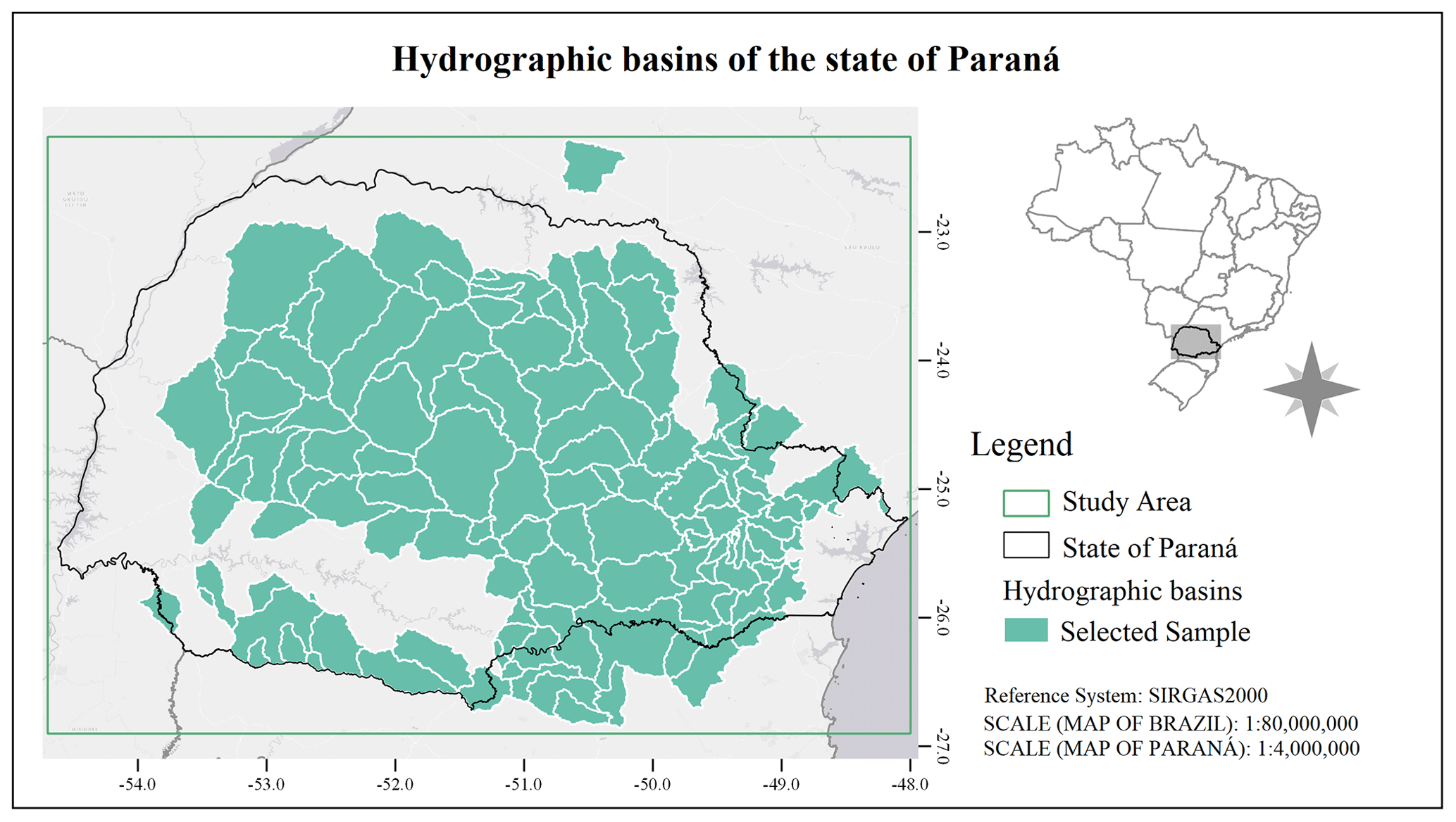
Figure 3 Location of selected watersheds in the state of Paraná.

3 Methods

The application of the physiographic–climatic similarity method implicitly considers two assumptions. The first assumption is that, if there is similarity between basins, there are similar hydrological responses. The second assumption is that the similarity between sets of calibrated parameters of the hydrological model between two or more river basins may reflect the similarity in terms of their behaviour in relation to the transformation of rainfall into flow (Oudin et al., 2008, 2010; Parajka et al., 2005; Blöschl et al., 2013). Spatial proximity assumes that neighbouring basins have similarities in climate, soil type, land use and cover, slope, altitude, and other characteristics (Arsenault et al., 2019). Non-linear regression models seek to equate the relationship between dependent variables (e.g. hydrological model parameters) with different independent variables (e.g. descriptive characteristics; He et al., 2011).

After the dataset construction, calibration and validation of the GR4J model was performed in all basins. The hydrological model, GR4J (Génie Rural à 4 paramètres Journalier), proposed by Perrin et al. (2003), has been implemented in different countries, such as France (Oudin et al., 2008, 2010), Australia (Pagano et al., 2010), Brazil (Neto et al., 2021), South Korea (Shin and Kim, 2016), Mexico (Arsenault et al., 2019), and Russia (Ayzel et al., 2019). This parsimonious model has been showing promising results and stands out due to its dependence on only a few parameters and its use of two meteorological forcing variables on a daily scale; these variables are the total precipitation and potential evapotranspiration averaged at the basin scale, requiring historical series of observed flows for the adjustment of its four parameters. Three regionalization methods of the GR4J constants were tested; they are based on (i) physiographic–climatic similarity, (ii) simple spatial proximity, and (iii) non-linear regression. Estimates of Q₉₅ flow using a machine learning algorithm based on the dataset were also compared with data. All these methods are explained in next subsections.

3.1 Calibration and validation of the hydrological model

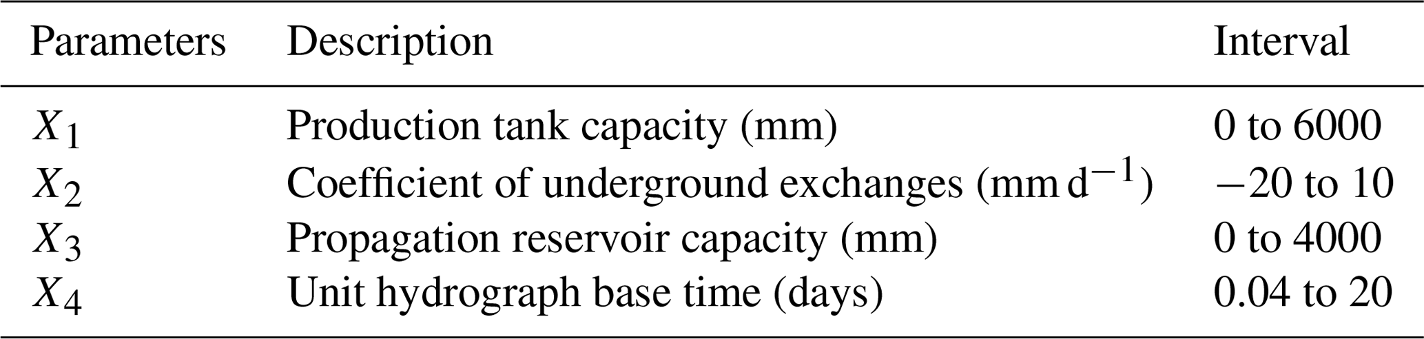
GR4J model parameters are obtained through calibration, a process of making simulated flow be as close as possible to observed flow. Table 1 summarizes the minimum and maximum values used for searching each constant of the model.

Table 1 Descriptions and ranges for GR4J model parameters.

The simulation period was divided into three parts: warm-up, calibration, and validation. The first 5 years of the simulation were used as a warm-up to eliminate the uncertainties in the initial conditions (Daggupati et al., 2015). The calibration and validation periods were defined as 70 % and 30 %, respectively, of the remaining time series after the warm-up.

The differential evolution (DE) optimization method was used for GR4J calibration. This method was initially proposed by Storn and Price (1997) and is part of SciPy library in Python. DE is used in optimization problems that use a single objective function, as in our case. According to Krause et al. (2005) and Muleta (2012), the use of the Nash–Sutcliffe logarithmic coefficient (logNSE) as an objective function is more influenced by low flows; therefore, this metric can be used to evaluate the performance of minimum-flow predictions. The logNSE can range from −∞ (poor fit) to 1.0 (perfect fit) and is calculated as follows:

$$\begin{array}{}\text{(1)}& \log \mathrm{NSE}=\mathrm{1}-{\displaystyle \frac{\sum _{i=\mathrm{1}}^N{\left(\ln \left(Q_i^{\mathrm{sim}}+\mathrm{0.001}\right)-\ln \left(Q_i^{\mathrm{obs}}+\mathrm{0.001}\right)\right)}^{\mathrm{2}}}{\sum _{i=\mathrm{1}}^N{\left(\ln \left(Q_i^{\mathrm{obs}}+\mathrm{0.001}\right)-{\stackrel{\mathrm{‾}}{Q}}_{\ln }^{\mathrm{obs}}\right)}^{\mathrm{2}}}},\end{array}$$

where $Q_i^{\mathrm{sim}}$ and $Q_i^{\mathrm{obs}}$ correspond to simulated and observed flow on day i, respectively. The average term ${\stackrel{\mathrm{‾}}{Q}}_{\ln }^{\mathrm{obs}}$ is calculated by ${\stackrel{\mathrm{‾}}{Q}}_{\ln }^{\mathrm{obs}}=\frac{\mathrm{1}}{N}\sum _{i=\mathrm{1}}^N\ln (Q_i^{\mathrm{obs}}+\mathrm{0.001})$.

Other metrics used to evaluate the performance of regionalization methods are the Pearson correlation coefficient (R); the Nash–Sutcliffe coefficient (NSE); and the Nash–Sutcliffe square root coefficient (sqrtNSE), where flow is transformed by the square root.

3.2 Regionalization methods

In this work, classical regionalization techniques based on physiographic–climatic similarity, simple spatial proximity, and non-linear regression were used. Regionalization based on physiographic–climatic similarity starts by identifying and grouping the watersheds that have the greatest physical, climatic, and geographic similarities. The purpose of clustering is to identify homogeneous regions based on descriptive indexes. Regionalization based on simple spatial proximity considers the fact that the study region is homogeneous and, therefore, that nearby basins are similar based on climate, relief, vegetation, landscape, and soil type. Although both assume that physical similarities can be closely correlated with hydrological responses, if the region is heterogeneous, regionalization based on physiographic–climatic similarity transfers information between basins that are not necessarily geographically neighbours. A second assumption to be considered is that the similarity between parameters from two or more river basins may reflect on the similarity of their behaviour in relation to the transformation of rainfall into flow (Oudin et al., 2008, 2010; Parajka et al., 2005; Blöschl et al., 2013). On the other hand, regression methods consider the fact that hydrological model parameters may be related to some physical processes that occur in watersheds and, consequently, are associated with some descriptive characteristics (Arsenault et al., 2019). In this way, it is possible to build a regression model for each parameter of the model.

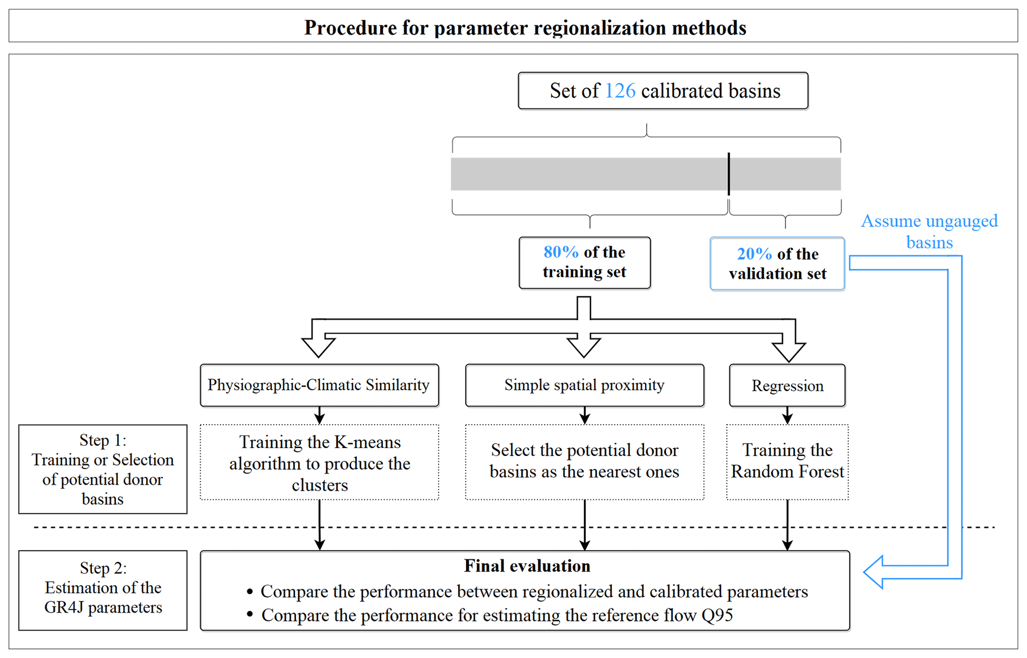
The diagram in Fig. 4 briefly summarizes the application of regionalization methods in this work. After calibrating the GR4J model for each of the 126 river basins, catchments were randomly divided into training and validation sets, with 80 % of the initial sample basins comprising the training set and 20 % forming the validation set.

The training set is formed by river basins considered to be possible donors of GR4J parameters and which were also used to train and build regionalization models. Basins of the validation set are considered to be pseudo non-instrumentalized (indicated by the blue arrow in the diagram of Fig. 4), even if it is known that these catchments have hydro-meteorological data and were calibrated. Each of the regionalization methods consists basically of different methodologies for selecting donor basins for transferring the parameters of the GR4J model to target basins.

Figure 4 Diagram summarizing the regionalization methods.

3.2.1 Physiographic–climatic similarity

When applying methods of predictions in ungauged basins (PUBs), we must take into account the uniqueness of each region across the globe and all the available information in each dataset. Bearing in mind the uniqueness of each location, possible basin descriptors were carefully chosen so that they would synthesize different characteristics of river basins and would be capable of transmitting the diversity between catchments within the same sample. Thus, the following descriptors were initially selected: basin area, length of main river, altitude and average basin slope, latitude of the basin centroid, daily averages of precipitation and potential evapotranspiration, aridity index, average number of days with extreme precipitation events and fraction of area covered by forest, and agriculture and urbanization.

Descriptors were normalized so that the mean and standard deviation corresponded to 0 and 1, respectively. This procedure ensures that different variables share the same scale without significant loss of information and, thus, allows categories with different magnitudes to be compared equally. Then, characteristics that showed variability, i.e. that described the set of watersheds as being heterogeneous, were selected.

Table A1 shows the descriptive statistics adopted; it reveals that Paraná basins have diverse areas, main-river lengths, and average altitudes. On the other hand, the fraction of urban area showed little variation; despite this, it was preferable to keep this descriptor since urban infrastructure, as well as other anthropogenic activities, can seriously disturb the processes of the hydrological cycle.

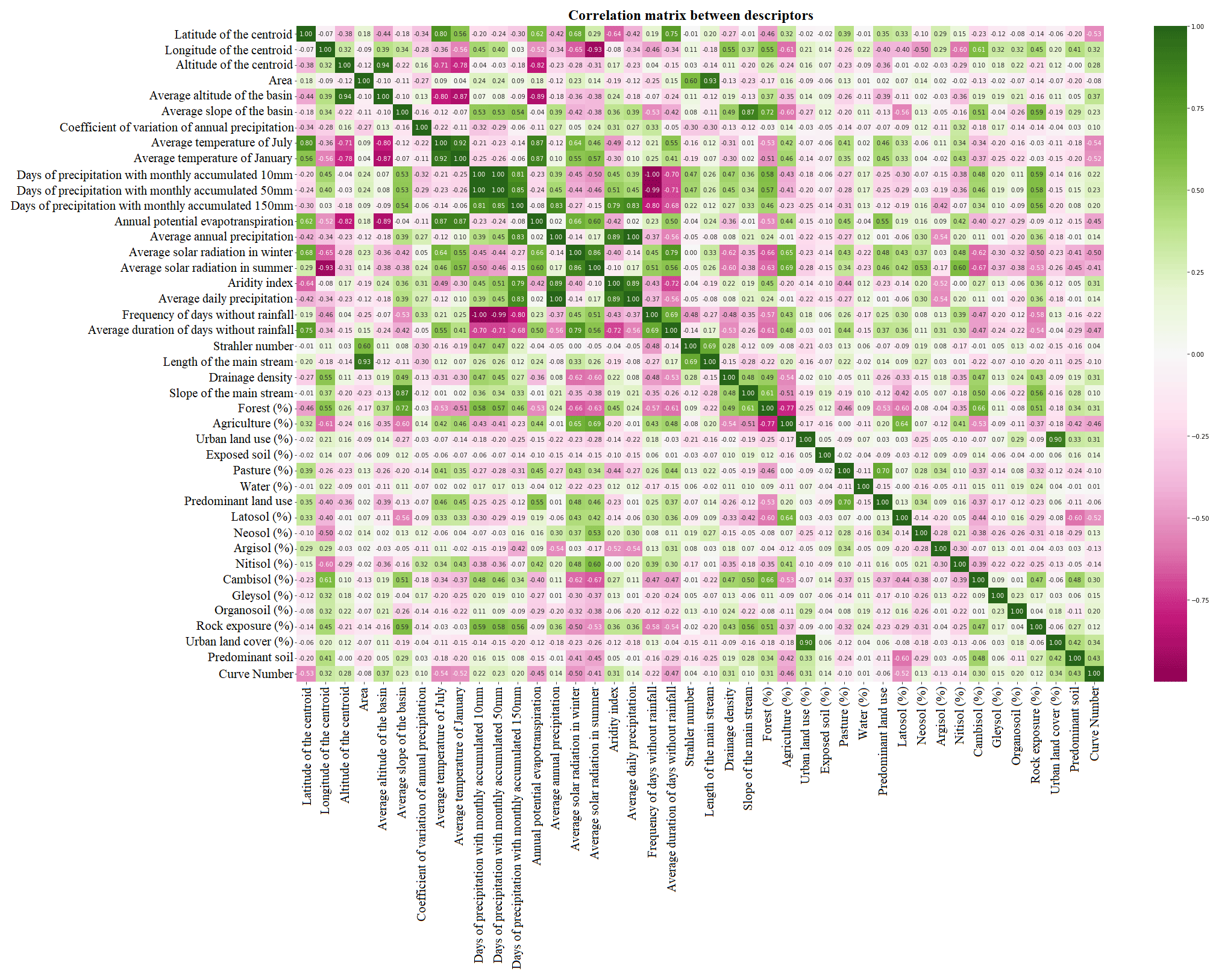
High multicollinearity between the descriptors can lead clustering algorithms to make wrong decisions during the formation of groups (Boutsidis et al., 2014). Therefore, two analyses were performed to identify the correlation between descriptors. First, the Pearson correlation (R) between each pair of descriptors was calculated. Second, the variance inflation factor (VIF) was determined to measure the degree of multicollinearity between descriptors. VIF ranges from 1 (when there is no multicollinearity) to infinity (when there is perfect multicollinearity); the threshold used in this work was below 5. Correlations between descriptors can be seen in Fig. B1. High correlations, with R values above 0.70, were found between the following pairs of descriptors: aridity index and days of monthly accumulated precipitation above 150 mm, average duration of days without rain and latitude of basin centroid, average slope of the basin and fraction of forest, fraction of agricultural area and fraction of forest, and annual potential evapotranspiration and average altitude of the basin. To reduce the dimensionality of data, the following descriptors were selected: area, forest fraction, urban area fraction, average duration of extreme events with high precipitation (days of monthly accumulated precipitation above 150 mm), and average duration of days without rain.

The Euclidean distance (dist), calculated using Eq. (2) below, is a metric that can express similarities (small distances) or differences (large distances) between n attributes of two basins (a and b) in an n-dimensional space of attributes (Viviroli et al., 2009).

$$\begin{array}{}\text{(2)}& {\displaystyle }\mathrm{dist}(a,b)=\sqrt{\sum _{k=\mathrm{1}}^n{\left[{\mathrm{atrib}}_k\left(a\right)-{\mathrm{atrib}}_k\left(b\right)\right]}^{\mathrm{2}}}\end{array}$$

Clusters were produced using the K-means method, which was implemented using the scikit-learn package. The application of the K-means algorithm involves the following: first, define the number of K groups; second, for each group, initialize a centroid randomly within the range of each category; third, assign each point to the centroid that has the smallest Euclidean distance with respect to the point; four, compute a new location of K centroids based on the average of all points assigned to it. The iterative process from the third to the fourth step is repeated until there are no more changes in the centroids (Wilks, 2011).

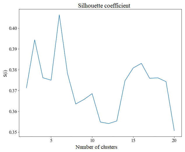
The value of K directly affects how groups will be formed. Increasing the number K leads to more groups, but consequently, each group will have fewer members (which brings homogeneity but does not guarantee representativeness). On the other hand, creating fewer groups generates groups with more members (which does not allow proper identification of the different groups). Two ways to evaluate if the appropriate number of clusters resulting from the agglomeration method is using the silhouette coefficient (Si) and the elbow method.

According to Rousseeuw (1987), the silhouette coefficient (Si) consists of calculating the average Euclidean distance (a_p) of a point p, with all points belonging to the same group. Then, the average distance (b_p) of the point p with respect to all the points belonging to the nearest neighbouring group is calculated. Thus, the coefficient can be determined using the following equation:

$$\begin{array}{}\text{(3)}& \mathrm{Si}={\displaystyle \frac{b_{\mathrm{p}}-a_{\mathrm{p}}}{\max \left(b_{\mathrm{p}},a_{\mathrm{p}}\right)}}.\end{array}$$

Si can vary between $[-\mathrm{1},\mathrm{1}]$, and the closer to 1 it is, the more distant the point p is from the neighbouring group. Values close to 0 indicate that the point p is close to the limit that divides both groups, and measurements close to −1 indicate that the point p may have been associated with the wrong group.

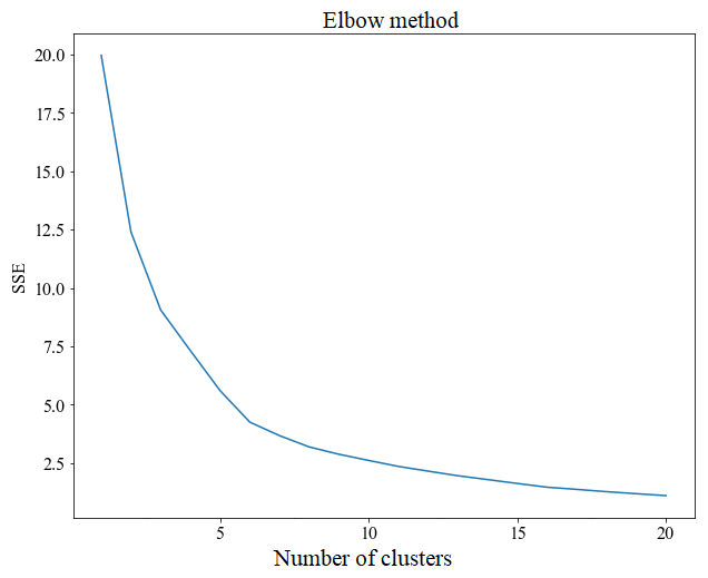
The elbow method is a graphical tool for evaluating an optimal number of clusters. This technique involves calculating an agglomeration coefficient; in this work, the criterion used was the sum of the squared distances of each sample (x_i) and the respective centroid (μ_j) of the grouping that the sample is part of, which can be expressed as the sum of squared errors (SSE):

$$\begin{array}{}\text{(4)}& \mathrm{SSE}=\sum _{i=\mathrm{1}}^n{\left(x_i-{\mathit{\mu }}_j\right)}^{\mathrm{2}}.\end{array}$$

As number of clusters grows, distances between samples and their respective centroids decrease. However, the number of groups and the clustering coefficient are expected to be small. Thus, from a graph with the agglomeration coefficient on the y axis and the number of groups on the x axis, it is possible to identify the point at which there is a sharp flattening or a rapid drop in this coefficient, suggesting an optimal number of clusters (Ketchen Junior and Shook, 1996).

3.2.2 Simple spatial proximity

The distance between two points – in this case, the centroids of target and donor basins – that have known latitudes and longitudes can be calculated using the Haversine distance, D_H:

$$\begin{array}{}\text{(5)}& \begin{array}{rl}{D}_{\mathrm{H}}=& \mathrm{2}r\arcsin \\ & \left[\sqrt{{\sin }^{\mathrm{2}}\left({\displaystyle \frac{x_{\mathrm{1}}-x_{\mathrm{2}}}{\mathrm{2}}}\right)+\cos \left(x_{\mathrm{1}}\right)\cos \left(x_{\mathrm{2}}\right){\sin }^{\mathrm{2}}\left({\displaystyle \frac{y_{\mathrm{1}}-y_{\mathrm{2}}}{\mathrm{2}}}\right)}\right],\end{array}\end{array}$$

where D_H refers to the distance in kilometres; r is the average radius of the Earth (approximately 6371 km); and x and y are, respectively, the latitudes and longitudes of points 1 and 2.

3.2.3 Regression

Multiple regression models, whether linear or non-linear, seek to find the best relationship between a dependent variable and independent variables; this is done by finding the minimum error given a target. In our case, the GR4J model parameters are dependent variables which will be calculated based on descriptive characteristics of the basins (independent variables). The non-linear regression method of random forests (Breiman, 2001), which was chosen for this work, is able to perform well when dealing with large datasets and is able to distribute weights for the independent variables according to their degree of importance. Thus, two types of regression methods were constructed: random forest I and random forest II.

Random forest I used 1000 decision trees and was trained using basin descriptors. For this technique, it is necessary to produce a regression model independently for each parameter (X₁, X₂, X₃, and X₄); however, the parameters of a hydrological model generally present dependent relationships among themselves and sometimes cannot be observed independently. Thus, a second method, defined as random forest (RF) II, included the calibrated parameters of training basins as descriptors. The second method followed the following steps: (i) a correlation analysis between GR4J parameters was performed, and, thus, an ordered list of parameters from highest to lowest correlation index was created, and (ii) a first regression was done for the parameter with the lowest correlation index – in this case, only the descriptive characteristics were used to train the model. Then, regression was performed for the parameter with the second lowest correlation index; here, we used descriptive characteristics and the previous parameter that had the lowest correlation index. This process was followed until all the parameters had their regressions.

3.3 Q₉₅ flow estimate

Instituto Água e Terra (IAT), the environmental agency responsible for legal permissions for the use of water resources in the state of Paraná, uses the river flow with 95 % permanence (Q₉₅) as a reference flow rate for permission licenses for water use (AGUASPARANÁ, 2010). We have proposed estimating Q₉₅ flow through regression techniques based on basin information and, thus, comparing it with Q₉₅ flow calculated using regionalized simulated flows. The construction of permanence curves involved (i) ordering the flows Q in ascending order for N days; (ii) assigning to each ordered flow Q_m the corresponding ranking order m; (iii) computing the frequency or probability of the ordered flows Q_m to be equalled or surpassed (P(Q≥Q_m)), which can be calculated using the Weibull plot position shown in the following equation (Pugliese et al., 2014):

$$\begin{array}{}\text{(6)}& P\left(Q\ge Q_m\right)=\mathrm{1}-{\displaystyle \frac{m}{N+\mathrm{1}}}.\end{array}$$

After obtaining Q₉₅ reference flows for the training set, a transformation of units (from m³ s⁻¹ to L s⁻¹ km⁻²) was performed, ensuring that the variable is not dependent on basin area. Then, another random forest regression method was trained and evaluated for the test set. This RF used 1000 decision trees and watershed descriptors that presented weights greater than 0.01.

As terminology may sound ambiguous, here, it is important to distinguish the training and test (or validation) sets used throughout this work. There are warm-up, calibration, and validation periods for river flow simulation, and there are also training and validation sets for machine learning performance evaluation. The 126 basins were divided into training and validation sets for regionalization evaluation. Also, for estimating GR4J parameters and Q₉₅ reference flows, additional training and test (or validation) sets were created for applying random forest regressions.

4 Results

4.1 Performance of the GR4J model

The GR4J model showed acceptable performances for the sample of 126 watersheds, as shown in Fig. 5, with about 65 % of Paraná watersheds presenting logNSE equal to or greater than 0.70 during the validation period. Basins located close to the Paraná coastline reached a lower efficiency when compared to other regions. Some river basins presented superior performances in the validation period when compared to the calibration period; however, inverse situations also occur. These phenomena may be associated with changes or improvements in measurement techniques, as well as being influenced by changes in land use and land cover.

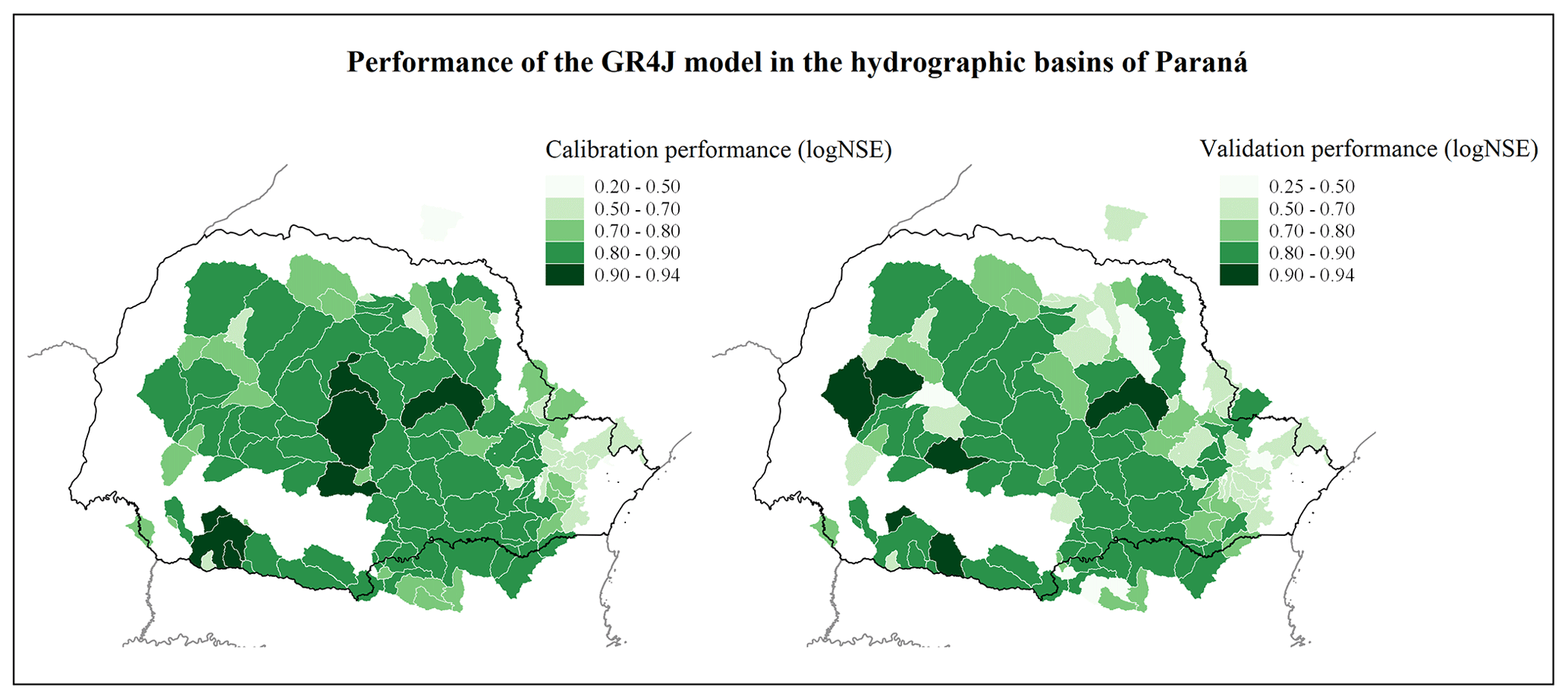
Figure 5 Performance of GR4J model during calibration and validation periods.

4.2 Performance of regionalization methods

The results of each regionalization method are described below.

4.2.1 Physiographic–climatic similarity

The regionalization method by physiographic–climatic similarity starts with defining the number K of clusters used to group the basins. The elbow method indicated that K=6 was appropriate, which is the point of abrupt slope change or curve flattening in Fig. 6. Accordingly, the silhouette coefficient (Si) was higher when the number of clusters K was equal to 6, as shown in Fig. 7. After defining K, we used 80 % of the 126 watersheds for training the K-means algorithm, which was used to group similar watersheds. The remaining 20 % were used to test and evaluate the clusters formed.

Figure 6 Elbow method for training set basins with K ranging from 1 to 20.

Figure 7 Silhouette coefficients for training set basins with K ranging from 1 to 20.

The geospatial distribution of watersheds and clusters formed by the K-means algorithm can be seen in Fig. 8 for basins in the training set (Fig. 8a) and validation set (Fig. 8b). Watershed location per group in the training set was similar to the basin spatial distribution in the validation set. Additionally, geographically close basins do not always belong to the same formed group.

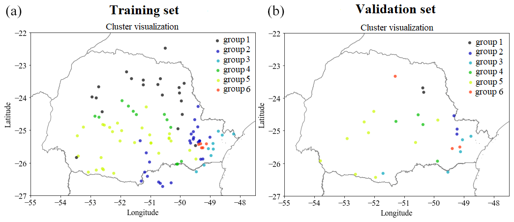
Figure 8 Clusters produced by the K-mean method for the 100 training basins (a) and 26 validation basins (b).

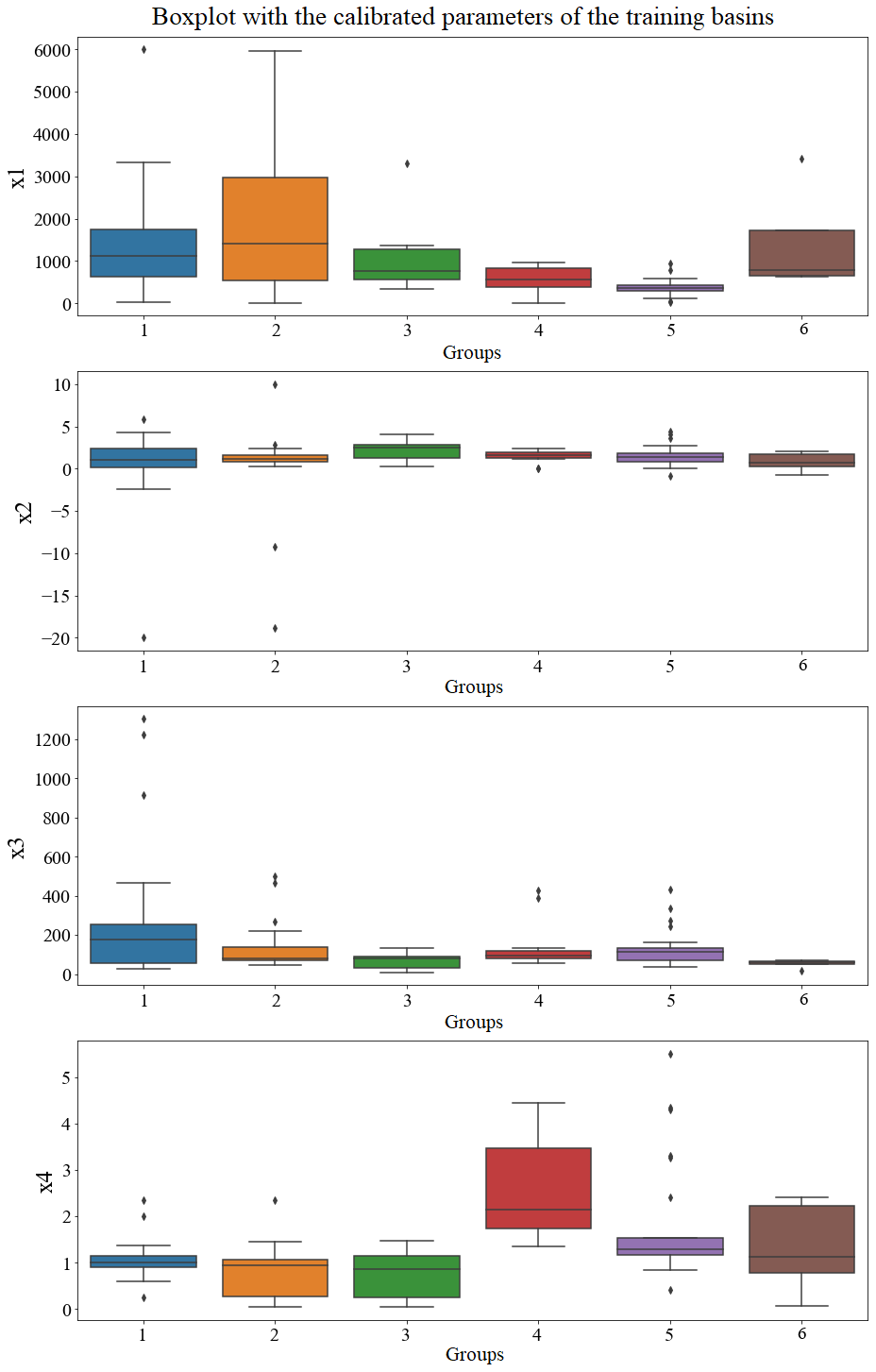
Descriptor distributions for each group in the training set are shown in boxplots in Fig. 9. Group 4 contains basins with the largest drainage areas, located in the second and third plateaus in the centre of the state of Paraná. Group 5 contains basins that have smaller drainage areas when compared to group 4, but these end up sharing similar characteristics to catchments in group 4. Groups 2 and 3 have a higher percentage of forests, but group 3 has a greater tendency to have more rainfall, smaller areas, and shorter periods of consecutive dry days. On the other hand, group 1 stands out for containing the basins that have the longest average duration of consecutive dry days. Finally, group 6 stands out from the others because it contains basins with the highest percentages of urban area and, therefore, may be more influenced by anthropogenic activities. Although the descriptors point to heterogeneities between the formed groups, it is still possible to see overlaps, mainly in relation to the calibrated parameters of the GR4J model, as shown in Fig. 10.

Figure 9 Basin descriptor distributions for training set clusters.

Figure 10 GR4J parameter distribution for basins in training set groups.

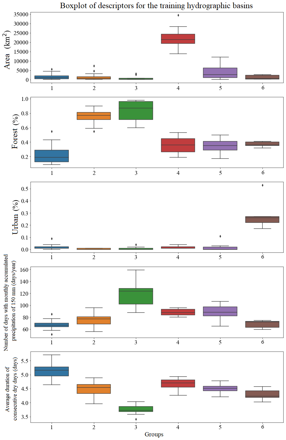
Basins from group 2, which are located on both the first and second plateaus of the state of Paraná, are similar in size to the basins of group 1 but have a higher percentage of forest as a distinct characteristic. Basins of group 3 are found mainly in the Paraná coastal region, near Serra do Mar, a long system of mountain ranges and escarpments, where orographic rain is more likely to occur. Group 5, which is present in greater quantity, contains hydrographic basins located in all plateaus of the state.

Looking at parameter distributions (Fig. 10) from a process perspective, we can find some relations with the catchment descriptor distributions (Fig. 9). Parameter X₁ represents the runoff-producing capacity of the watershed reservoir. Our result shows that group 2, which has a higher percentage of forests, also has the highest X₁ median and spread. This can support the hypothesis that more forest may improve the catchment capacity for generating runoff. Parameter X₄ represents the base time of the instantaneous unit hydrograph. The boxplots show that larger basins (group 4) have higher X₄ parameters; i.e. bigger watershed areas may increase the base time of a hydrograph. Parameter X₃ represents the propagation reservoir capacity. Our results show that group 6, which has more urban areas, also has the smaller X₃ parameter. This reflects the effect of city impermeabilization in terms of the flow propagation capacity; i.e. after a precipitation event, the watersheds with more urban area have a smaller propagation capacity or a fast response in terms of the flow peak.

4.2.2 Simple spatial proximity

The simple spatial proximity regionalization method considers the fact that the region near the basin of interest is homogeneous and that it therefore has hydrological similarity. Assuming this hypothesis to be true, we have used the Haversine distance between pairs of receiving basins (pseudo-non-monitored) and donor basins (instrumented basins) to transfer parameters from the GR4J model. In both methods, namely physiographic–climatic similarity and simple spatial proximity, the receiving basins are all catchments within the validation set, and the possible parameter donor basins are those from the training set that reached logNSE equal to or greater than 0.70 during the validation period.

We have allowed more than one donor basin to transfer the GR4J parameters to target basins. When there is more than one donor catchment, the four parameters of each donor basin were used to estimate flow in the pseudo-non-instrumented target basin. Once the flows were simulated with the donor basin parameters, the averages of modelled flows were calculated and used for the target basin.

We compared the ability of both methods (spatial proximity and physiographic–climatic similarity) to generate good results in parameter regionalization. For this, we varied the number of donor catchments from 1 to 10 and evaluated the median logNSE of the receiving-catchment river flow simulations in the validation period. The analysis to identify the number of donor basins, shown in Fig. 11, indicates that the similarity method presented a maximum median logNSE for a total of one basin, and the proximity method presented better results using seven basins as donors.

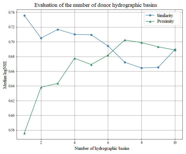
Figure 11 Evaluating the optimal number of donor basins based on logNSE medians during the validation period of receiving-basin simulations. The green and blue lines represent spatial proximity and physiographic–climatic similarity regionalization methods, respectively.

4.2.3 Regression of GR4J parameters

To train the random forest regression model, known information about the watersheds in the training set was used, namely the descriptive characteristics (independent variables) and the calibrated parameters of the GR4J model (dependent variable). The descriptive characteristics that the random forest pointed out to be most relevant were the slope of the main river and the average slope of the basin for parameter X₁, the average altitude and the average radiation in winter for parameter X₂, the average radiation in winter for parameter X₃, and the fraction of Gleissol for parameter X₄. These reinforce that machine learning algorithms perform better with physiographic–climatic indices as inputs.

4.3 Q₉₅ flow estimation

In order to compare the performance of estimating the Q₉₅ reference flow between direct (regression) and indirect (regionalization of parameters) techniques, the regression method of random forest, which was named random forest Q₉₅, was applied to directly regionalize Q₉₅ flow.

The construction of the random forest Q₉₅ regression model used known information about the watersheds in the training set, namely the watershed descriptor (independent variables) and the Q₉₅ (in L s⁻¹ km⁻²), estimated from the observed historical series (dependent variable). The most relevant characteristics identified by the random forest Q₉₅ method were days of precipitation with monthly accumulation of 150 mm, basin centroid longitude, basin average slope, pasture fraction, and forest fraction. Q₉₅ was calculated, for both observed and simulated flows, using calibration and validation periods. Thus, at least 15 years of fluviometric records were used to estimate the reference flow.

Correlations between observed Q₉₅ flows and those predicted by calibration and regionalization methods were calculated. Regionalizations with the highest performances were obtained by the physiographic–climatic similarity method, with a correlation (R) of 0.973, and then the random forest Q₉₅ method, with a correlation of 0.965. Q₉₅ flows predicted by calibration of the GR4J model had a correlation of 0.9956, the regionalization method based on proximity had a correlation of 0.9386, and the random forest method reached a correlation equal to 0.9392.

5 Discussion

In dry periods, the flows of rivers in Paraná are sustained basically by two mechanisms: baseflow and groundwater recharge. Even in periods with no precipitation, there can be movements of water from underground aquifers and saturated soil layers into surface waterbodies, such as rivers, lakes, or wetlands. All basins studied in this research drain into the Paraná River, beneath which there resides the Guarani aquifer, one of the largest sandstone aquifers in the world (Hirata and Foster, 2021). Karst terrains are also widespread throughout the Paraná basin, with the Açungui karst and non-carbonate karsts being the most important ones (Auler and Farrant, 1996; Vestena and Kobiyama, 2007). The Açungui carbonate karst is characterized by large areas of horizontally bedded limestones and dolomites, which form extensive regions of little or no relief and are drained by low-gradient rivers (Auler and Farrant, 1996). Interbasin groundwater flow may also play an important role in the water balance during dry periods in karst catchments (Vestena and Kobiyama, 2007).

Bartiko et al. (2019) identified that the rainfall season occurs in the months of December, January, and February in the south of Brazil. The basins under study in the state of Paraná are in a region of climatic transition, with reasonably well-distributed rainfall throughout the year. The region's seasonality is generally divided between the 6 months centred around summer, from October to March, which correspond to the wet period, and the remaining months, from April to September, which correspond to the dry period. However, the occurrence of cold fronts, low-pressure areas, and instability systems during the Brazilian winter can provoke large floods – even though this is the dry period – and interrupt the recession process of the hydrographs.

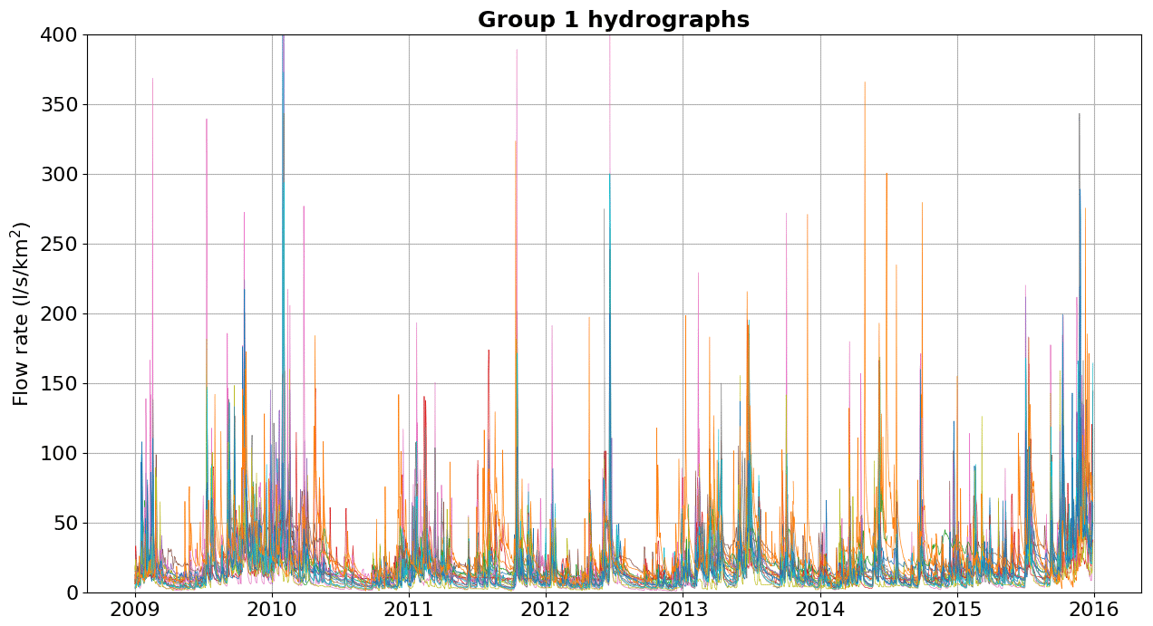
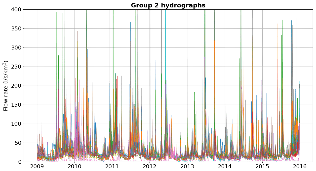
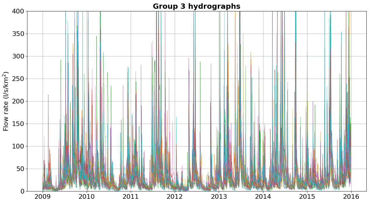
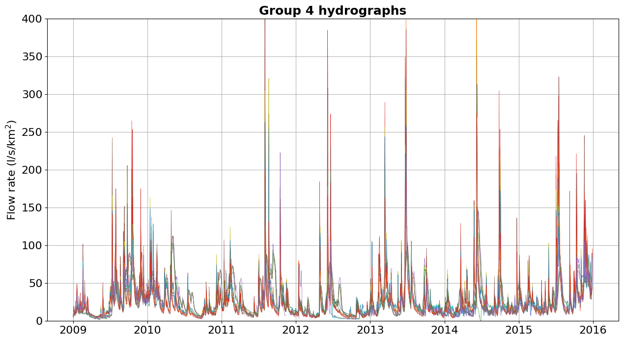
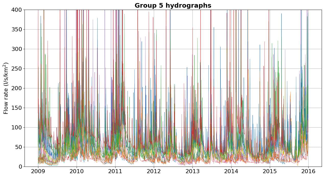
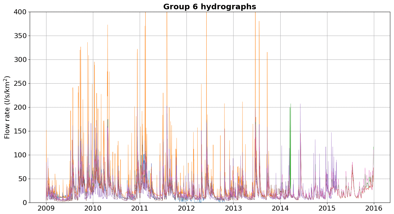
In Appendix C, we show the hydrographs by physiographic–climatic similarity group. The comparison of hydrographs separated by groups of similar watersheds show the seasonality and strength of smaller flow rates. In these climatic conditions, the predominance of low flows is expected from April to September. The slow release of groundwater volumes after the cessation of surface runoff causes a recession curve that is strongly influenced by river–aquifer interaction. This curve, which conceptual models try to capture through simple mathematical relationships, is influenced by various factors, namely soil properties, hydraulic characteristics and the extent of aquifers, the rate and amount of groundwater recharge, evaporation and evapotranspiration of the basin, and the spatial distribution of vegetation cover, among others (Musy et al., 2014).

Due to the complexity of hydrological processes and the specificities existing in the river basins, representing the recession curve and simulating low flows using conceptual models is an arduous process, sometimes requiring a basin-by-basin hydrological analysis. Attempts to improve this representation in the design of hydrological models have resulted in an increase in parameters, as is the case of traditional Sacramento Soil Moisture Accounting (SAC-SMA) model, which uses two conceptual reservoirs to simulate low flows with an overlay effect that allows us to better capture low-flow variability for a wider range of river basins (Burnash, 1995). The model applied in our study has an improved version, the GR6J, dedicated to low flows, which uses two additional parameters to better represent exchanges between the river and groundwater (Pushpalatha et al., 2011). In both cases, a better representation of low flows is achieved at the cost of increased model degrees of freedom, which is not ideal for regionalization issues.

In general, the vast majority of basins from the validation group presented results with logNSE greater than 0.50 for different regionalization methods, and only two basins within this group presented low performance. Another general behaviour was that basins with logNSE equal to or greater than 0.77 using calibrated parameters also achieved comparable performances with regionalized parameters. Additionally, in some cases where regionalization methods used more than one donor basin, they provided a diversified set of parameters. When combining this set of parameters, GR4J with the average of each parameter can result in superior performance compared to the use of calibrated parameters in a period prior to validation.

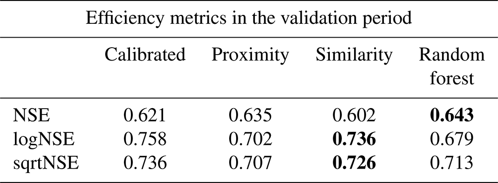
Results were evaluated using the Pearson correlation coefficient (R), the Nash–Sutcliffe coefficient (NSE), and their variations: the flow transformed by the square root (sqrtNSE) and by the logarithm (logNSE). NSE gives more emphasis to the performance of higher flows, logNSE is more sensitive to low flows, and sqrtNSE provides an intermediate performance (Oudin et al., 2008). Table 2 shows the median values of error statistics for estimated flows in the validation period of the 26 watersheds from the validation set. Among the regionalization methods, values that achieved the best results for each index are highlighted in bold. Thus, the physiographic–climatic similarity stands out positively by reaching logNSE and sqrtNSE equal to 0.736 and 0.726, respectively. Another point to be highlighted is that the spatial proximity method presents, in general, median results for the three coefficients. Table 2 also reveals that regionalization method performances – in particular for proximity and random forest – can reach median NSE values equal to or greater than when parameters were calibrated in a period prior to validation.

Table 2 Median values of error statistics calculated for validation period. In bold are the best results for each index among the regionalization methods.

The review carried out by Guo et al. (2020) included the analysis of articles from different regions of the globe, which were recently published between 2013 and 2019 and in which the researchers also applied similar regionalization techniques (proximity, similarity, and regression). The same authors show evidence that regionalization methods based on distances (proximity and similarity) generally present superior performances compared to methods based on regression. The study carried out by Kuentz et al. (2017) in Europe explored the correlation between 16 different indices of hydrological-behaviour responses (e.g. baseline flow index, Q₅ and Q₉₅) and 35 physical descriptors (e.g. area, slope, and aridity index), concluding that there are strong connections between the physical descriptors and the response rates of the hydrological behaviour.

Mohamed et al. (2019) explain that, due to the non-linear and multidimensional relationship between basin descriptive characteristics and model parameters, the application of regression methods that use machine learning techniques are becoming more common to extrapolate hydrological model parameters. In our study, random forest methods performed better when the average radiation in winter and the days of precipitation with monthly accumulation above 150 mm were used to inform the algorithm, which reveals key variables required for understanding regionalization techniques in humid subtropical and hot temperate climates.

6 Conclusions

In this study, three regionalization methods were developed and deployed with the purpose of estimating daily flows in basins of the state of Paraná. A set of hydrometeorological data was created and presented together with catchment descriptive indexes. The amount of collected data is greater than that of national-level datasets for the region since a higher density of fluviometric stations was used. GR4J was employed for 126 watersheds and achieved optimistic performances in the validation period (logNSE ≥ 0.70) for 65 % of the watersheds.

All regionalization methods showed positive performances. Median values of logNSE in regionalizations were equal to 0.702, 0.736, and 0.679 for spatial proximity, physiographic–climatic similarity, and random forest methods, respectively. When comparing the median NSE between the three methods, random forest is slightly better. However, the median sqrtNSE was higher for the physiographic–climatic similarity method. The regionalization based on physiographic–climatic similarity proved to be the most robust method for predicting daily flow and Q₉₅ reference flow. When increasing the number of donor basins, the method based on spatial proximity has comparable performance to the method based on physiographic–climatic similarity.

Based on the physiographic–climatic characteristics of the basins, it was possible to classify six distinct groups of watersheds in Paraná. Basins within each group showed similarities in their size, urban-area fraction, average duration of consecutive dry days, number of days with more than 150 mm of precipitation, and forest fraction. Interestingly, the last two descriptors were also relevant for the random forest Q₉₅ model. The use of machine learning algorithms to regionalize streamflow had good performance using climatic and physiographic indices as inputs. This research represents a proof of concept that basins without flow monitoring can have a good approximation of streamflow if physiographic–climatic information is provided.

Our regionalization study showed that parameters are sensitive to basin physiographic characteristics and soil use, and this has a direct effect on the streamflow response, i.e. hydrograph peak time, hydrograph base time, production capacity, and propagation capacity. Urban impermeable areas produce a fast response in terms of the flow peak. Forests play a significant role in groundwater recharge and low-flow generation through various mechanisms: interception and slowing infiltration, enhancing soil structure and porosity, and reducing erosion through root system soil stabilization. Overall, forests act as natural sponges, slowing down the movement of water, enhancing infiltration, and promoting groundwater recharge. Protecting and maintaining forest ecosystems is essential for sustaining groundwater resources and ensuring water availability for both human and natural systems.

We recommend for future studies the use of stochastic optimization techniques for model calibration and the use of different hydrological models for parameter regionalizations. In addition, we suggest the estimation of confidence intervals for the regionalized parameters and the use of regionalization methods based on geostatistical techniques. Another recommendation is to include flow seasonality indices (Burn et al., 1997; Parajka et al., 2010) as descriptors to better characterize the physiographic–climatic similarity of the basins.

Appendix A: Data availability and physiographic–climatic indices

Figure A1 shows the availability of data over the years; the darker the shade of green, the more data. Watershed descriptive characteristics are shown in Table A1. Note that the region can be classified as having a humid subtropical climate (Matallo Junior, 2001).

Table A1 Descriptive statistics for the Paraná dataset.

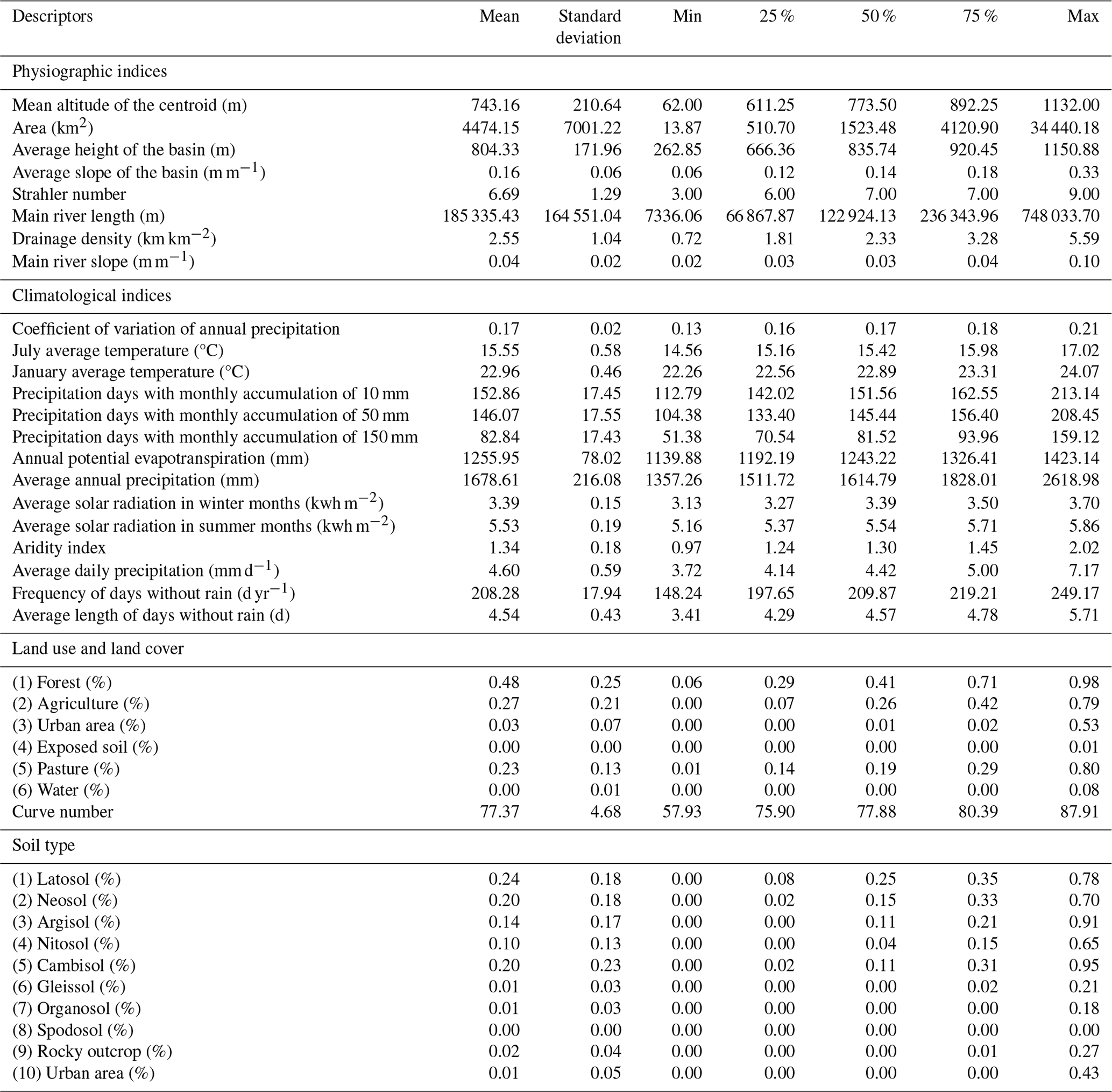
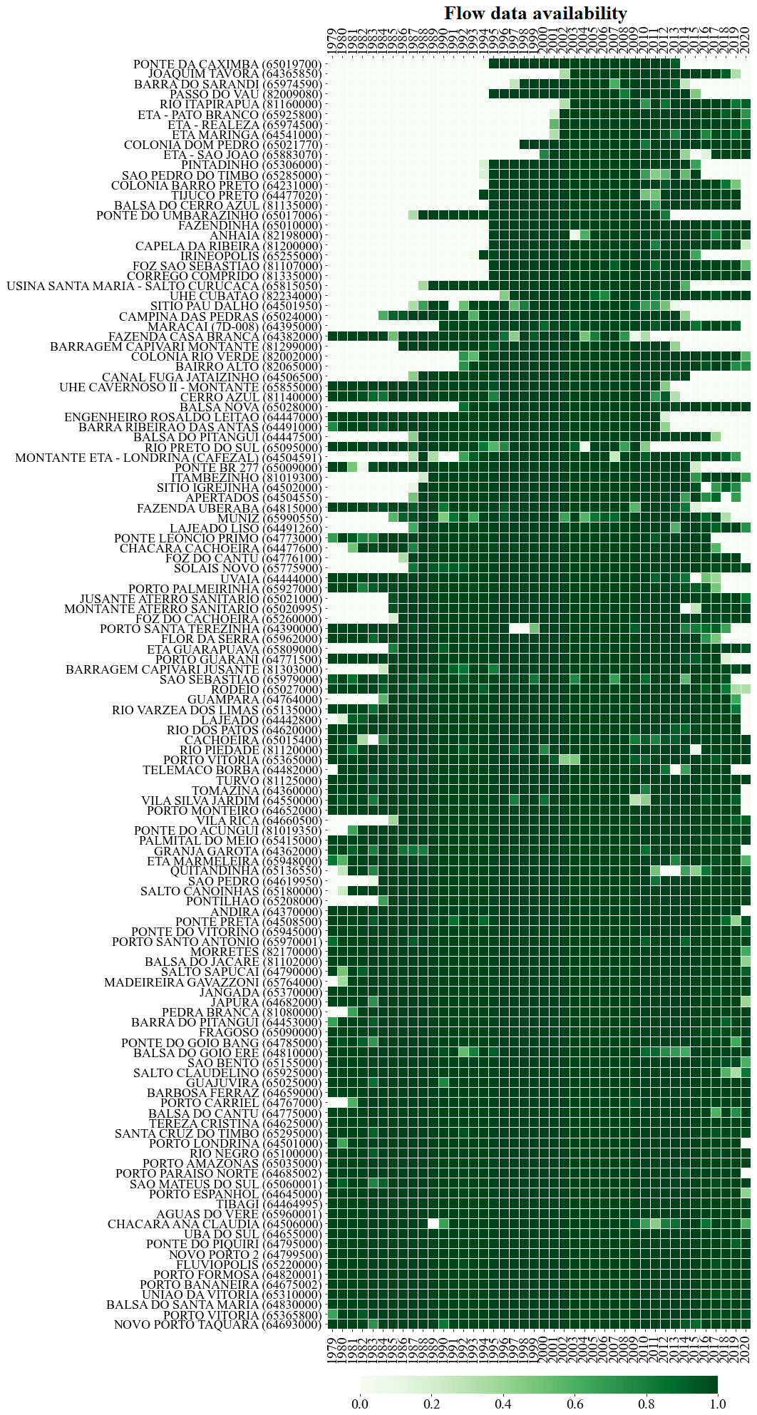
Figure A1 Availability of flow data by station. The darker the green colour is, the more data are available for that year.

Appendix B: Comparison of descriptors

Figure B1 shows the Pearson correlation coefficients between watershed descriptors.

Figure B1 Pearson correlation coefficients between descriptors.

Appendix C: Hydrographs by physiographic–climatic similarity group

Below, we show the hydrographs separated by groups of watersheds with physiographic–climatic similarity. The hydrographs were produced based on flow records observed from 2009 to 2016, and the y axis was limited to 400 L s⁻¹ km⁻² for comparison. Figures C1–C6 show hydrographs from the catchments of groups 1, 2, 3, 4, 5, and 6, respectively.

Figure C1 Hydrographs from basins of group 1.

Figure C2 Hydrographs from basins of group 2.

Figure C3 Hydrographs from basins of group 3.

Figure C4 Hydrographs from basins of group 4.

Figure C5 Hydrographs from basins of group 5.

Figure C6 Hydrographs from basins of group 6.