the Creative Commons Attribution 4.0 License.
the Creative Commons Attribution 4.0 License.
 | 15 Jul 2024
Regional patterns and drivers of modelled water flows along environmental, functional, and stand structure gradients in Spanish forests
Jesús Sánchez-Dávila
Miquel De Cáceres
Jordi Vayreda
Javier Retana
The study of the water cycle in the forest at large scales, such as countries, is challenging due to the difficulty of correctly estimating forest water flows. Hydrological models can be coupled with extensive forest data sources, such as national forest inventories, to estimate the water flow of forests over large extents, but so far the studies conducted have not analysed the role of stand structure variables or the functional traits of the forest on predicted blue and green water flows in detail. In this study, we modelled the water balance of Spanish forests using stand structure and species data from forest inventories to understand the effects of climate, stand structure, and functional groups on blue water flows. We calculated blue water and green water flows and expressed them relative to received precipitation. Relative blue water flow was mainly concentrated in the wetter regions (Atlantic and alpine biomes) of Spain (around 25 %) in comparison with the Mediterranean biomes (10 %–20 %) and during the autumn–winter season. The leaf area index (LAI) of the forest stand is the most important predictor of relative blue water, exhibiting a negative effect until it reaches a plateau at higher levels (around 2.5–3). Deciduous forests showed a greater relative blue water flow than evergreen functional groups (25 %–35 % and 10 %–25 %, respectively) primarily due to leaf fall during the autumn–winter season. This study highlights how green water is decoupled from blue water; namely, blue water depends on winter and autumn precipitation, while green water depends on the spring and summer water demand and how the species' functional traits (deciduous vs. evergreen) can influence blue water production.
- Article
(6675 KB) - Full-text XML
-
Supplement
(2253 KB) - BibTeX
- EndNote


Forests are one of the most important ecosystems on the planet and constitute a supplier of carbon and water for humanity (MEA, 2005). Even though water is the main determinant of vegetation worldwide (Wang-Erlandsson et al., 2022), the water cycle is particularly challenging to study because it is difficult to measure its components. The water cycle in forests depends on the precipitation that falls in the forest, which can be partitioned into the green water and the blue water (Caldwell et al., 2016; Schlesinger and Jasechko, 2014). The green water is the evapotranspiration flow from the forest to the atmosphere formed by the water transpired by plants together with the evaporation of intercepted precipitation by vegetation and the evaporation from the soil surface (Llorens et al., 2011). Climate, specific traits, stand forest structure, and their interactions determine the partitioning of precipitation between green water and blue water. Forest evapotranspiration is determined by local climate conditions, such as air temperature, radiation, vapour pressure deficit, or soil water availability (Granier et al., 2000). Moreover, plant transpiration is different among species depending on their specific traits, as leaf area and xylem traits determine the efficiency of water transport or leaf phenology (evergreen and deciduous) (Ford et al., 2011). Stand forest structure is also key in rainfall partitioning through its relationship with stand leaf area index (LAI; total area of leaves of the canopy per unit horizontal ground area), which is a key variable determining transpiration (Granier et al., 2000) and/or the interception of vegetation. On the other hand, blue water can be split into two flows: the surface runoff and the surplus of groundwater by the system and available downstream.
Green water reduces the amount of blue water produced at a local scale but recycles the water through evapotranspiration at a global scale (Ellison et al., 2012). Green water flow is usually greater than blue water's in forests and grasslands in comparison with croplands or wetlands due to the greater transpiration of the former (Oki and Kanae, 2006). Green water represents around 40 %–70 % of water flow in temperate and boreal forests (Schlesinger and Jasechko, 2014), and even 90 %–100 % in drier environments or years, including Mediterranean forests (Ungar et al., 2013; Campos et al., 2016; Qubaja et al., 2020). The combination of different rainfall dynamics, transpiration, stand structure, and specific life traits can modify the partitioning between green and blue water. For instance, water yield can be affected by the temporal distribution of rainfall events (seasonality and torrentiality). Relative water interception by trees decreases when rainfall increases, being greater in arid environments compared to humid forests (Levia and Frost, 2003). In Mediterranean forests, the interception is greater than in temperate forests due to the smaller amount of rainfall and intensity and the higher evaporation caused by the higher temperature (Limousin et al., 2008). However, evaporation of intercepted water is lower during late-summer intense convective storms since the rainfall intensity is very high and lasts a short time (torrentiality) (Llorens and Domingo, 2007). Physiological and phenological differences among species also modulate water flows. Evergreen Mediterranean trees can reduce their transpiration in summer (water saver), but deciduous trees increase it due to higher water demand (water spender) (Baquedano and Castillo, 2006; Klein, 2014; Link et al., 2014; McDowell et al., 2008). Therefore, Mediterranean forests show transpiration seasonality, with a reduction in stomatal conductance during the summer drought, while the transpiration in temperate forests follows leaf phenology more closely (Llorens et al., 2011).
Water balance in forests has been studied mainly at local and landscape scales, like in watersheds (Caldwell et al., 2016; Guzha et al., 2018; Schwärzel et al., 2020) or forest stands (Benyon et al., 2017; Simonin et al., 2007). Analyses at regional scales have also been carried out (Hoek van Dijke et al., 2022; Mastrotheodoros et al., 2020; Sun et al., 2005), analysing the water flow variation by topoclimate or landscape vegetation cover with hydrological models. The study of water fluxes in forest ecosystems is an important challenge for forest management. Ecohydrological simulations have been shown to be a valuable tool to understanding water fluxes at different spatial scales, complementing the limited field data available (Hoek van Dijke et al., 2022; Mastrotheodoros et al., 2020). The effect of stand structure variables on the water flow have been studied at a local scale with field data (Benyon et al., 2017; Simonin et al., 2007). Nevertheless, landscape-level ecohydrological simulations have been most often carried out without incorporating the role of the stand structure variables or the differences in species and functional composition (Hoek van Dijke et al., 2022; Mastrotheodoros et al., 2020).
In our study, we analysed the spatial pattern and partitioning of blue and green water in Spain using ecohydrological simulations with the MEDFATE water balance model (De Cáceres et al., 2023, 2015), which uses detailed field stand structure and species composition derived from forest inventory data. We simulated water flows and their green and blue water components at a daily resolution, and we studied the spatial distribution of relative blue water and its seasonality. Spain is an adequate region to study the partitioning between blue and green water because it shows contrasting climate gradients in terms of temperature, amount of rainfall, and seasonal distribution. Importantly, it includes a contrasted climate between the Mediterranean area – with hot temperatures, low precipitation, and seasonal drought – and the temperate area – with warm temperatures and a higher amount of rainfall and without seasonal drought (Rivas-Martínez et al., 2011). In addition, peninsular Spain harbours both temperate and Mediterranean forests that span a broad gradient of forest types and stand structures that can modify the partitioning between blue and green water. The questions addressed by the study are as follows: (1) which are the spatio-temporal patterns of blue and green water throughout the Spanish Peninsula and among climate subregions? (2) How does this partitioning between blue and green water vary among contrasting forest functional groups? (3) Which are the main climatic and forest structural drivers of this partitioning between blue and green water?
2.1 Study area
The studied area spans the forested areas of Spain, including the Iberian Peninsula and the Balearic Islands, but excluding the Canary Islands. This encompasses two climatic domains: the temperate climate with Atlantic Sea influence in the north and west parts of the Iberian Peninsula and the Mediterranean climate on the rest of the territory. The temperate climate is wetter and colder, while the Mediterranean climate is hotter and drier. We have classified the Iberian territory into six biomes (see map in Fig. S1 in the Supplement) according to the Iberian climate classification of Allué Andrade et al. (1990): (i) arid (9.0 % of the Spanish surface), with warm winters and summers and very low precipitation (< 400 mm); (ii) temperate Mediterranean (34.8 %), which is hot in winter and summer with low precipitation (400–600 mm); (iii) continental Mediterranean (30.9 %), which is cold in winter and hot in summer with low precipitation (400-600 mm); (iv) sub-Mediterranean (11.0 %); which is cold in winter and hot in summer with wetter precipitation (about 800 mm); (v) Atlantic (10.5 %), characterized by a mild winter and summer and high precipitation (> 1000 mm); and (vi) alpine (3.8 %), which is very cold in winter and cool in summer and characterized by high precipitation (> 1000 mm).
2.2 Forest inventory data
We used the permanent field plots from the Spanish national forest inventories to characterize the predominant species and stand structure variables across the study area. The Spanish national forest inventories (SFIs) are distributed with a systematic survey along the forested areas with a density of ∼ 1 plot km−2. Specifically, we used the third inventory (SFI3) carried out in 1997–2008, which is the most recent and complete survey available to date. Spanish permanent field plots have four concentric circular subplots with radii of 5, 10, 15, and 25 m. Trees were identified and measured within variable circular size plots (5 m radius for trees with diameter at breast height (dbh) ≥ 7.5 cm, and trees with 2.5 ≤ dbh ≤ 7.5 cm are counted; 10 m radius for trees with dbh ≥ 12.5 cm; 15 m radius for trees with dbh ≥ 22.5 cm; and 25 m radius for trees with dbh ≥ 42.5 cm). Moreover, the shrub species or genus within the 10 m radius subplot was measured with its corresponding percent cover value and average height.
We focused on the field plots with > 70 % of plot basal area of the most predominant tree native species (Table S1) and an overall basal area of > 3 m2 ha−1 (to ensure that very sparse woodlands, which can hardly be considered a forest, were excluded), resulting in a total number of plots of 32 514. Plots were classified according to the dominant species in terms of basal area into five functional groups: temperate (e.g. Fagus sylvatica) and Mediterranean deciduous forests (e.g. Quercus pyrenaica), temperate (e.g. Pinus sylvestris) and Mediterranean coniferous forests (e.g. Pinus pinea), and sclerophylls (e.g. Quercus ilex) (see Fig. S3 for the SFI3 map of the plots selected and Table S1 for the classification of the tree species into these five groups).
2.3 Environmental variables
We downloaded the daily data of total precipitation and maximum, mean, and minimum temperature for the 5 years before and after the date of survey for every plot (that is, 10 years per plot) from E-OBS data at a 1 km horizontal resolution (Moreno and Hasenauer, 2016); ftp://palantir.boku.ac.at/Public/ClimateData/ (last access: 2 February 2023). Topographic variables of slope, aspect, and altitude were derived from a digital elevation model (DEM) at 25 m2 of the Spanish National Orthophoto Program (PNOA) through the Instituto Geográfico Nacional (IGN) website (https://centrodedescargas.cnig.es/CentroDescargas/index.jsp#, last access: 14 February 2022). We used these topographic variables to obtain daily values of the relative humidity, solar radiation, and potential evapotranspiration (PET) per plot through the meteoland R package (De Cáceres et al., 2018). We characterized plot-level climatic conditions using three climatic indexes: climatic moisture (mean annual precipitation / mean annual PET), continentality (mean temperature of the hottest month with the mean temperature of the coldest month subtracted), and precipitation seasonality (standard deviation of monthly precipitation / mean of monthly precipitation) multiplied by 100).
A summary of the main stand structure and climate characteristic of the different functional groups and biomes is shown in Table S2.
2.4 MEDFATE model
The MEDFATE model (version 2.9.3) has been designed to simulate plant water balances and soil in structurally and compositionally heterogeneous forest stands (De Cáceres et al., 2015, 2023). MEDFATE uses daily weather as input and most processes are simulated at daily time steps. The aboveground stand structure is represented in terms of total crown ratio (CR), height (H), and leaf area index (LAI) of a set of woody plant cohorts. The soil is represented by vertical layers with different hydraulic properties, and each cohort may have a different root distribution specified using the depth corresponding to cumulative 50 % and 95 % of fine roots (Z50 and Z95, respectively).
Each day, the model updates the leaf area for (semi-) deciduous vegetation based on a simple phenological model that dictates and leaf drop. This model relies on the degree days required for leaf budburst (SGDD) parameter, representing the degree days needed for budburst (assuming evergreen plants maintain a consistent leaf area throughout the simulation). Subsequently, the model revises the light attenuation within the canopy, adhering to the Beer–Lambert model, as well as the canopy's water storage capacity, which signifies the minimum water quantity required to saturate the canopy. Following the canopy status update, the model addresses the input of water from precipitation. Prior to augmenting the soil layers' water content, the model initially deducts the water loss from rainfall due to interception and surface runoff. Rainfall interception loss is estimated using the simplified version of the Gash model (Gash et al., 1995), while runoff is calculated according to the United States Department of Agriculture Soil Conservation Service (USDA SCS) curve number method (Boughton, 1989). Processes related to lateral water transfer are omitted from consideration. Soil water storage capacity and water potential are derived from soil texture through pedotransfer functions (Saxton et al., 1986). When replenishing a specific soil layer, a portion of the water is assumed to directly infiltrate the layer below, as determined by microporosity (Granier et al., 1999). The water percolating from the deepest layer is presumed to be lost through deep drainage.
To assess plant transpiration, the model initially calculates a distinct estimation of the maximum transpiration for the entire plant community (including trees and shrubs) – that is, without considering the soil water deficiency. This calculation is done for each taxon and takes into account the atmospheric evaporative demand. It involves two taxon-specific parameters: and parameters. The estimation of maximum transpiration for the entire stand (Emax,stand(i)), excluding considerations for soil water deficit, relies on the daily Penman potential evapotranspiration (PET) and an empirical relationship established by Granier et al. (1999). However, MEDFATE modified the Granier equation with and :
where and represent species-specific parameters (De Cáceres et al., 2023). Assuming reliable species-specific estimates are accessible for and , the equation can be applied to calculate Emax,stand(i). Once Emax,stand(i) is determined for each species in the stand, the portion of shortwave radiation absorbed is employed to estimate its maximum transpiration (Emax(i)) from Emax,stand(i) (Korol et al., 1995).
Moreover, the cohort's transpiration is influenced by the vertical distribution of fine roots, the soil moisture profile, and two parameters specific to the taxon: Ψ extract and c extract. These parameters represent the soil water potential at which 50 % of the maximum transpiration occurs and the slope of a Weibull function that regulates the rate of transpiration decline, respectively. The plant's water status is expressed as plant water potential, denoted as Ψ plant, which is defined as the “average” of the soil water potential in the rhizosphere. The model monitors the effects of drought by assessing the proportion of hydraulic conductance lost due to stem cavitation, referred to as PLC. Increases in PLC occur whenever Ψ plant decreases, following a xylem vulnerability curve characterized by the parameters VC_stemc and VC_stemd. PLC sets limits on actual transpiration rates and does not decrease even when Ψ plant increases. It is worth noting that the effects of cavitation can only be reversed, i.e. PLC can be reduced, through the formation of new sapwood, as outlined by Choat et al. (2018).
2.5 Parameter estimation
Data from forest inventory plots included tree height (H) and tree diameter at breast height, which were used to obtain estimates of foliar biomass (henceforth leaf area, after multiplying by the specific leaf area, SLA) and crown ratio (CR) via species-specific allometries (see Tables S1–S3 of De Cáceres et al., 2023, for more details). In shrubs, foliar biomass is calculated from shrub height via species-specific allometries. In the model, SLA (specific leaf area; in mm2 mg−1), the ratio of leaf area to leaf dry mass, is constant for every species (De Cáceres et al., 2023). The leaf area index (LAI; in m2 m−2) was calculated from the foliar biomass (in kg m−2) using a specific leaf area coefficient (SLA; in m2 kg−1) that is species-specific (LAI = foliar biomass ⋅ SLA). Taxon-specific parameter details are shown in the supplement of De Cáceres et al. (2023). Soil data of each forest inventory plot were extracted from the SoilGrids database (Hengl et al., 2017). For all plots, four soil layers down to a total depth of 4 m were initially considered, but the deepest layers were merged into a rocky layer (95 % of rocks) following the depth of the R horizon. A monotonous increase in rock fragment content across soil layers from the surface to the rocky layer was defined based on surface stoniness classes determined in SFI3 plot surveys.
2.6 MEDFATE simulations
MEDFATE was run on each selected SFI3 plot using daily weather data (temperature and precipitation, PET, and radiation and relative humidity) corresponding to a 10-year period centred on the year of the SFI3 sampling (1997–2008). We calculated the blue water as the sum of the runoff and deep water and the green water as the evapotranspiration (that included the sum of the transpiration, interception, and soil evaporation).
2.7 Model evaluation
MEDFATE predictions have already been evaluated at the forest stand scale in terms of soil moisture dynamics, plant transpiration, and water status in Mediterranean forests (De Cáceres et al., 2021, 2015). Given the focus of the present work, we evaluated regional-scale patterns of green and blue water predicted by MEDFATE against those produced by alternative methods. First, we did a comparison between the results for average blue water of MEDFATE with the average blue water from the Precipitation–Runoff Integrated Model (SIMPAL; the acronym is in Spanish) of the Spanish government. SIMPAL is calibrated with stations that measure streamflows across Spain, and it is interpolated at a 1 km2 resolution for the whole country (Estrela et al., 2012). Second, we compared green water patterns predicted by MEDFATE with those of GLEAM, which is derived from satellite data and covers the world at a resolution of 0.25° (Martens et al., 2017). We used the GLEAM v3.8a that defines the evapotranspiration as the sum of transpiration (from short and tall vegetation), interception (from tall vegetation), soil and open water evaporation, and snow sublimation.
2.8 Statistical analysis
Our analyses focused on the relative blue water, the ratio between simulated annual mean blue water, and the total precipitation as response variable. The variation in relative blue water across biomes and functional groups was analysed using beta regression models (Ferrari and Cribari-Neto, 2004). We used beta regressions because the response variable was a proportion. A post hoc Tukey's test was applied for pairwise comparisons between groups (i.e. biomes and functional groups).
The effect and importance of climate, topographic, and stand structure variables in the partitioning of blue/green water of every functional group were analysed with XGBoost regression. XGBoost is a machine learning system that builds a sequential series of shallow regression trees with a gradient boosting technique (Chen and Guestrin, 2016). XGBoost regression was used because it allows us to analyse linear and non-linear responses and correlated variables. A regression tree is trained by splitting the input dataset into increasingly homogeneous subsets at each decision node and choosing the split that maximizes the distance between different terminal nodes. As predictors, 14 different climatic variables calculated as the mean annual values of the 10 years of climate data for every plot (mean, maximum, and minimum temperature; solar radiation; and moisture and continentality indexes) and the mean of seasonal variables (precipitation of spring, winter, summer, and autumn and precipitation seasonality index) were used. A topographic variable (slope) and two stand structure variables (basal area and LAI of the plot) were also included. Basal area serves as an indicator of canopy cover, as it is calculated by summing the trunk cross-sectional area at breast height of all trees per hectare, and higher basal area values can result in increased interception. LAI determines the transpiration of the trees and shrubs through the leaf surface. LAI of the plot was calculated from the sum of the LAI of trees and shrubs. One model was computed for each of the five functional groups. The models were tuned for finding the best hyperparameters and they were evaluated using a k-fold cross-validation procedure (10-fold with five repetitions), following a stratified random sample into k subsamples of the dataset. A forward feature selection method for selecting the predictor variables with a spatial cross-validation (Meyer et al., 2018) was used. The models were built for each predictor pair combination and the best was selected. The remaining predictors were tested by adding them to the best combination. This procedure continued until neither of the remaining predictors resulted in an improvement of the model. Variable importance in the retained variables was evaluated by computing the fractional contribution of each feature to the model based on the total gain of these variable splits (gain), the relative number of times a feature is used in trees (frequency), and the relative value of the feature observation (cover). We estimated R2 to test the accuracy of the final models with 1 − (Sres/Stot), Sres being the sum of the squared differences between the observed values and the predicted values and Stot the total sum of squares, which is the sum of the squared differences between the observed values and the mean of the observed values. All statistical analyses were conducted with R v.4.1.1., with the packages xgboost (Chen et al., 2016) and caret (Kuhn, 2008).
3.1 Model evaluation
The comparison indicated that the blue water of SIMPAL and the green water of GLEAM followed the same regional patterns as MEDFATE (Fig. 1). SIMPAL reaches higher values of blue water in the Atlantic biome and lower values in west temperate Mediterranean than MEDFATE. In opposition, GLEAM evapotranspiration is higher in the west temperate Mediterranean and lower in the Atlantic forest than MEDFATE. MEDFATE models are at a stand scale, whereas SIMPAL and GLEAM models are at a regional scale. At a stand scale, the evapotranspiration is high in the Atlantic forest, and then the blue water is lower. The west temperate Mediterranean is characterized by forests of low basal area and LAI (Table S2; Fig. S4). Therefore, the evapotranspiration is lower and blue water higher than surrounding forest. In other words, the differences observed seem to arise from the fact that MEDFATE takes into account the stand structural characteristics, which are difficult to represent in models based on interpolation (SIMPAL) or remote sensing (GLEAM).
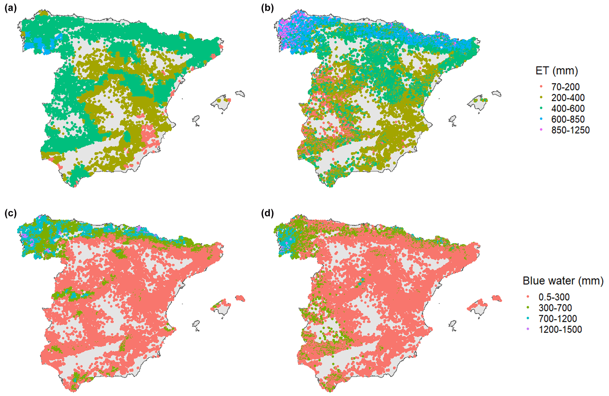
Figure 1Average evapotranspiration (ET) maps for SFI3 plots according to GLEAM (a) and MEDFATE (b) (Spearman correlation = 0.62; R2= 0.218) and average blue water maps for SFI3 plots according to SIMPAL (c) and MEDFATE (d) (Spearman correlation = 0.70; R2= 0.354).
3.2 Spatial patterns of blue water in the Spanish biomes
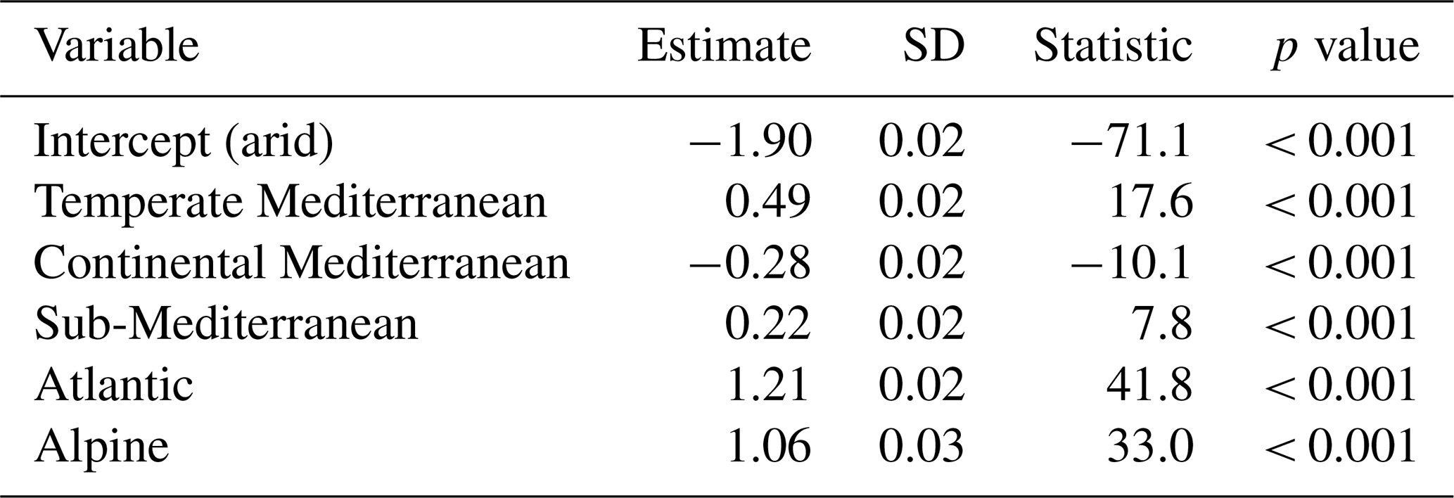
Forests with the highest absolute amount of blue water (> 500 mm) were mostly concentrated on the coast of the Atlantic Sea and in the Pyrenees (Fig. 2a). The south of the Spanish Peninsula in the temperate Mediterranean biome and some areas inside the continental Mediterranean biome had values between 300 and 500 mm. The rest of the country had lower blue water values (< 300 mm), mainly in the eastern and Mediterranean regions. Relative blue water showed a very similar spatial pattern, with the highest values located on the coast of the Atlantic Sea and the Pyrenees (Fig. 2b). In the southwest of Spain and in the Mediterranean mountain regions, the relative blue water was also high (> 50 %). Forests in the eastern Mediterranean region had the lowest values. The arid and continental Mediterranean biomes showed a very large percentage of plots (> 70 %) with low relative blue water (< 15 %), whereas the Atlantic and alpine biomes showed higher plots (> 50 %) with high blue water (> 30 %) (Table S3). Temperate Mediterranean and sub-Mediterranean biomes showed more intermediate values, although the temperate biome had the percentage of plots with the highest blue water (> 60 %) among all biomes. The results of the beta regression model and post hoc Tukey's test indicated that there were differences among biomes in the percentage of blue water (Table 1; Fig. 3; see Figs. S5–S6 for interception and soil evaporation differences): relative blue water was higher in the Atlantic and alpine biomes (mean over 25 %) followed by the temperate Mediterranean and sub-Mediterranean biomes, with the arid and continental Mediterranean biomes showing the lowest values (mean of 10 %–15 %). The absolute values showed a similar pattern to those of the relative blue (see Fig. S7).
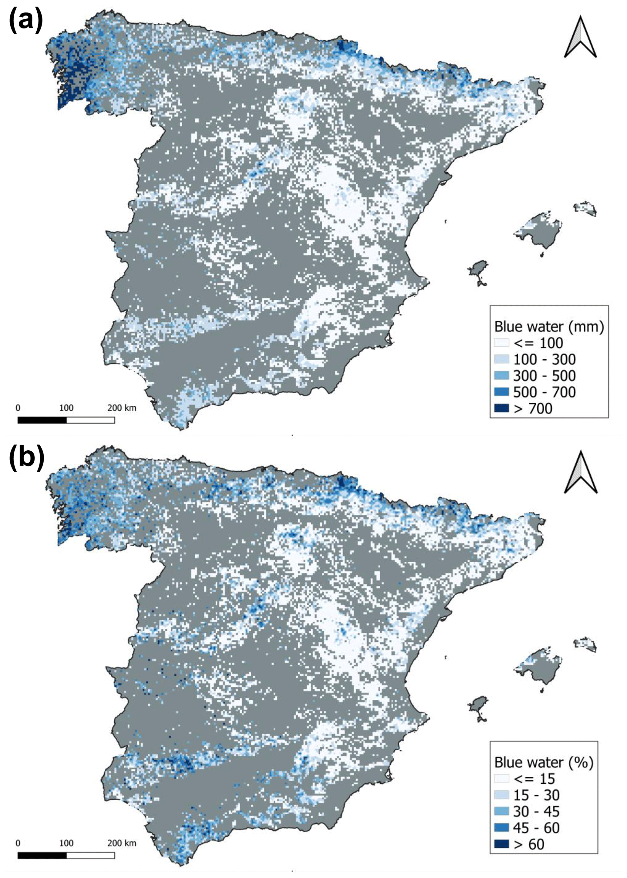
Figure 2Total (a) and relative (b) blue water in the Spanish Peninsula and Balearic Islands. In the grey area, no forest covers are shown. Maps were realized with a rasterization of the SFI3 plot results at 1 km2.
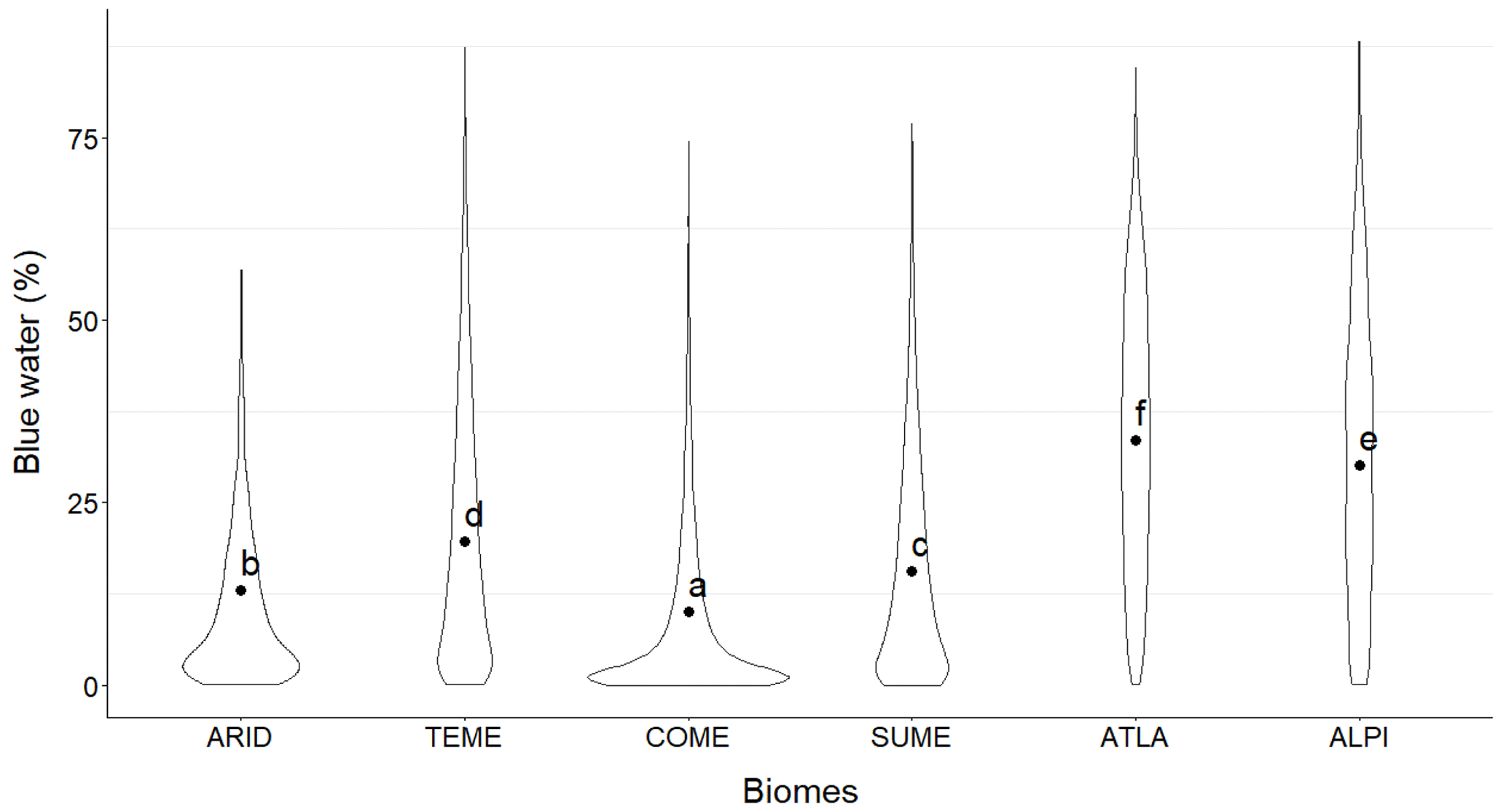
Figure 3Percentage of blue water in the different biomes. Different letters denote significant differences among biomes (p < 0.01) after Tukey's test. ARID: arid, TEME: temperate Mediterranean, COME: continental Mediterranean, SUME: sub-Mediterranean, ATLA: Atlantic, ALPI: alpine.
Table 1Results of the beta regression models regarding relative blue water (%) for the different biomes, indicating the estimate, standard deviation (SD), statistic, and p value of each of them. A positive value indicates that an increment occurred in the biome with respect to the observed values in the intercept.
3.3 Patterns of blue water among forest functional groups
Beta regressions models and post hoc Tukey's test indicated that there were also differences among functional groups in the percentage of blue water (Table 2; Fig. 4; see Figs. S8–S9 for interception and soil evaporation differences). Relative blue water was high in temperate deciduous forests (35 %) followed by temperate coniferous forests, Mediterranean deciduous forests, and sclerophylls (20 %–25 %). Mediterranean coniferous forests had the lowest value (close to 10 %). The absolute values showed a similar pattern to that of the relative blue with the temperate deciduous with the highest values (see Fig. S10).

Figure 4Percentage of blue water of the different functional groups of species. Different letters denote significant differences among forest types (p < 0.01) after Tukey's test. TEDE: temperate deciduous, MEDE: Mediterranean deciduous, TECO: temperate coniferous, MECO: Mediterranean coniferous, SCLE: sclerophylls.
Table 2Results of the beta regression models regarding relative blue water (%) for the different forest functional groups, indicating the estimate, standard deviation (SD), statistic, and p value of each of them. A positive value indicates that an increment occurred in the functional group with respect to the observed values in the intercept.

The analysis of seasonality using monthly aggregated data showed that the amount of blue water in forests of the different functional groups strongly varied throughout the year. In the temperate deciduous forests, total blue water was higher than total evapotranspiration in autumn and winter (Fig. 5a), whereas in other functional groups, the values of the two flows were similar throughout the year, except in spring–summer, when the green water was higher. In the Mediterranean coniferous forests, evapotranspiration was higher than blue water all year long. Relative flows showed that blue water was at its minimum in the summer season in all groups and higher than evapotranspiration only in autumn–winter in temperate deciduous forests (Fig. 5b).

Figure 5Total (a) and relative (b) green water and blue water and total precipitation by different functional groups throughout the year. Note that evapotranspiration can be higher than precipitation during summer months due to plant transpiration and bare-soil evaporation of water available in the soil. Relative evapotranspiration has been truncated to 100 % of precipitation with the aim to improve the visualization of water export. A line marks the seasons in the months.
3.4 Main drivers of the partitioning between blue and green water
XGBoost models showed high accuracy, with R2 > 75 % in most functional groups (Table S4). These analyses revealed that LAI was the most important predictor of relative blue water in all functional groups (Fig. 6). The second and third most important variables were the climatic moisture index and winter precipitation, except for Mediterranean deciduous forests, for which it was autumn precipitation (see Figs. S11–S12 for spatial variation in climatic moisture and winter precipitation). The other variables retained in the models had low significance.

Figure 6Average importance from gain, cover, and frequency values for every predictor variable retained in the XGBoost models for the five functional groups.
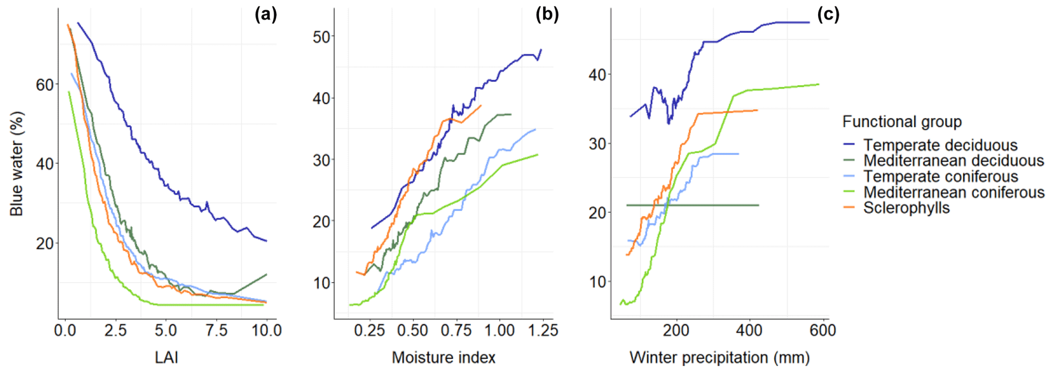
Figure 7Partial dependence plots for the three main predictor variables(a, LAI; b, climatic moisture index; c, winter precipitation) and their effect on blue water percentage for the different functional groups.
Partial dependence plots showed that LAI had a strong and negative effect on relative blue water (Fig. 7). Nevertheless, this effect was different depending on the functional group. The temperate deciduous forest showed the highest percentage of blue water for the whole LAI gradient, being always at a value of over 20 %. The other forest types showed similar patterns among them, with a larger drop until LAI was < 3 and values of around 10 % afterwards. The only exception was the group of Mediterranean conifers, which showed lower percentages of blue water than the other groups for the LAI gradient. The climatic moisture index showed a positive effect in all groups. The three angiosperm groups had a similar slope and showed higher values than the two gymnosperm groups (Fig. 7b). Winter precipitation had a positive effect on all functional groups except on the Mediterranean deciduous forests (Fig. 7c). Temperate deciduous forests showed higher values through the whole winter precipitation gradient.
4.1 Spatio-temporal patterns
Blue water spatial patterns showed that most Spanish forests have a proportion of the precipitation below 15 % as blue water (Fig. 3). This pattern was expected since most of the Spanish forests are in the Mediterranean climate, and in these dry environments, the evaporative demand is high and the majority of water evapotranspired or was intercepted by the canopy (Ungar et al., 2013). In contrast, in the Atlantic and alpine biomes, the proportion of rainfall as blue water can be higher than 25 % because these biomes are wetter and colder than the Mediterranean, and, thus, the evapotranspiration is lower and precipitation is higher (Kosugi and Katsuyama, 2007; Mastrotheodoros et al., 2020). Moreover, in some mountain areas in the continental Mediterranean biomes (e.g. Sierra Nevada and Sierra de la Demanda), the amount and proportion of blue water are also high (Fig. 2a, b). These regions are wetter than the rest of Mediterranean biomes and an increase in precipitation determines an increase in blue water (Helman et al., 2017). Interestingly, in other areas of southern Spain, in the temperate Mediterranean biome, the proportion of blue water can also be higher than 20 % (e.g. Sierra Morena; Table S3), not because they have higher rainfall but because this biome has very open forests, with LAI values lower than in the rest of biomes (Table S1). Transpiration is the main component of the green water in arid environments and decreases in wetter regions, where the interception increases their importance (see Fig. S13). This result is concordant with the global patterns of green water flux, where the transpiration is bigger in arid environments (Good et al., 2017).
The analysis of seasonal dynamics by forest type showed that in forests of all functional groups, there is more blue water during autumn and winter months. In contrast, the evapotranspiration was higher in spring–summer. In Mediterranean climates, there is a decoupling between rainfall and temperature (Baldocchi and Xu, 2007), with higher rainfall in spring and autumn and higher temperatures in summer. For this reason, plants have more photosynthetic activity and growth in spring (when rainfall is high) and more transpiration in summer (when temperature is the highest) (Baquedano and Castillo, 2006; Link et al., 2014), when trees use the groundwater stored in the soil (Jost et al., 2005). Water loss by runoff or deep drainage is higher in autumn–winter because water is not fully exploited by the forest in this lower-photosynthetic period, and, thus, green water is made lower than would be possible by falling rain (Helman et al., 2017; Williams et al., 2012). According to our results (Fig. 5), blue water is concentrated in this period of lower or dormant vegetation activity (i.e. late autumn and winter).
4.2 Differences in blue water between forest functional groups
The analysis of the percentage of blue water of the different functional groups of species showed that temperate deciduous forests had the highest value followed by Mediterranean deciduous forests (Fig. 4). The rest of forest types had lower values (Fig. 4), mainly in the case of Mediterranean coniferous forests, which have shown high green water of almost 90 %, as also observed in studies at the plot level (Ungar et al., 2013). The seasonal dynamics of these flows in the different forest types show that deciduous forests have more blue water in autumn and winter months than evergreen forests (Fig. 5). This indicates that the main factor that explains the differences in relative blue water between forest types is the shedding of leaves (or its lack of shedding) during the cold part of the year. Although deciduous trees are mainly water-spending since their transpiration is higher than that of evergreens (Baldocchi, 2020), they shed their leaves in autumn, and their interception and evapotranspiration are lower than those of evergreens in autumn/winter (Fig. 5). Moreover, due to their shape, coniferous needles intercept the rainfall more than the deciduous ones for the same area of leaves (Carlyle-Moses, 2004). Although green water is higher in deciduous than in evergreen forests in summer (Fig. 5), total annual blue water seems to be more determined by leaf phenology, which conditions the destination of the autumn–winter precipitation and determines the differences between deciduous and evergreen forests. Also, climate partial plots showed that at the same level of climatic moisture index and winter precipitation, deciduous forests have greater relative blue water than coniferous ones and sclerophylls (Fig. 7b–c).
However, once the differences between deciduous and evergreen forests are highlighted, the next aspect that stands out when comparing the different types of forests is that for each category of leaf phenology, the proportion of blue water depends mainly on climate. Thus, temperate deciduous forests have more relative blue water than Mediterranean deciduous ones (Fig. 4). Temperate deciduous forests, which are the ones exporting the most blue water in relation to their precipitation, are mainly concentrated in the Atlantic and alpine biomes, where precipitation is higher and transpiration is lower, while Mediterranean deciduous forests are concentrated in Mediterranean biomes, where precipitation is lower and transpiration is higher (Table S2). The same pattern happens in evergreen forests: temperate coniferous forests have a percentage of blue water that is higher than Mediterranean coniferous forests because precipitation in the biomes where they are more abundant is also higher than in the Mediterranean. The lowest value of blue water in Mediterranean coniferous forests is particularly relevant because this is the most abundant forest type in Spain, and it is predominant in Mediterranean biomes (Table S1). Finally, sclerophyll forests produce more blue water than Mediterranean coniferous forests although both are situated in Mediterranean biomes and are evergreen. Sclerophyll forests have higher transpiration than Mediterranean coniferous ones (del Campo et al., 2019; Sánchez-Costa et al., 2015), but the total LAI of their stands is lower (Table S2), which determines the different pattern obtained (as explained in the next section).
4.3 Differences in stand structure determining blue water
The analysis of the drivers affecting relative blue water showed that LAI is the most important predictor of blue water (Fig. 6). In our simulations, relative blue water was often very high (> 60 %) when LAI was < 1. Transpiration and interception are higher when the LAI of the stand is higher, and, therefore, the water is transpired and intercepted by leaves. However, the temperate deciduous forests showed higher blue water for the same LAI values. Deciduous trees present higher evapotranspiration than evergreens at the same level of LAI (Baldocchi et al., 2010), but, as described previously, the LAI effect is modulated by leaf phenology since blue water in these forests is concentrated in winter. When LAI is very low, evergreen forests can show higher relative blue water. For instance, the temperate Mediterranean biome showed a higher percentage of plots with a higher relative blue water than Atlantic or alpine biomes (Table S3) because the mean LAI of their forests is lower than in the rest of biomes (see Table S1). This points out the importance of stand structure and composition since in a drier environment, LAI values higher than 2–3 m2 m−2 can strongly reduce the relative blue water. This effect is higher if the forest is evergreen, which is the predominant type in the Mediterranean. Relative blue water of Mediterranean deciduous forests is higher than that of evergreens because a decrease in LAI in evergreen forests decreases tree transpiration but increases evaporation from the soil surface, which is high in the Mediterranean climate even in winter (Raz-Yaseef et al., 2010). The management of blue water in forests has been focused in modifying the basal area of the stand (del Campo et al., 2014). Nevertheless, in this study, basal area was a limited predictor of the blue water in comparison with LAI. LAI of the stand increases with basal area until a threshold, and then it remains stable (Fig. S14). Although the increase in basal area over time reduces blue water (Caldwell et al., 2016), a plateau is expected in the long term, since LAI will not increase more after a maximum is reached. For this reason, blue water did not reduce excessively when LAI was higher than 3 (Fig. 7a). The reduction in basal area in the forest through thinning is a recurrent way of increasing blue water (Ameztegui et al., 2017; del Campo et al., 2018; Simon and Ameztegui, 2023), but this non-linear relationship between basal area and LAI implies that only heavy management for reducing basal area would be effective for reducing the LAI of the stand and, thus, increasing blue water.
4.4 Limitations
Model simulations to estimate water flows are not the same as observing them and can lead to artificial results. In this sense, it is necessary to continue improving the ecohydrological model design parametrization to improve their accuracy, including the completion of traits of many species for the parametrization, a better soil database, or the inclusion of lateral water flows (in the case of the MEDFATE model). Model evaluation is another key aspect to increasing realism and usefulness of predictions. The model MEDFATE has been validated in Mediterranean forests on a local scale with field ground data, but it has not been validated on a country scale with field data like eddy flux or sap flow data, and it might have lower accuracy in the Atlantic or alpine biome or with some tree species. Nevertheless, the comparison between MEDFATE results and other land surface products showed similar regional patterns. Despite accepting these limitations, the lack of field data at bigger scales encourages the use of models to study water flows on a country or continental scale.
Ecohydrological models like MEDFATE allow us to model different species and stand structures, improving our insights into the role of forests in water flows. Thus, we can split the fluxes of water at a stand level and understand the role of species, climate, and stand structure variables in the different water flows: transpiration, interception, runoff, etc. Moreover, the incorporation of forest inventories into these models allows us to conduct analyses at large spatial scales across multiple climates, forest typologies, and species compositions. In the current context of global change, the knowledge of water fluxes in forests is essential to being able to define strategies to improve the water budget, especially in dry environments like the Mediterranean, where water is scarce and the previsions are in line with increasing drought periods. Thus, in the context of global change, we are suffering (Hoerling et al., 2012; Lionello et al., 2014), the low amount and proportion of blue water in a major part of Spain is an important problem in the water supply for the agriculture or human consumption in the region (Ellison et al., 2012). The consequences that this lack of blue water might have on the entire silvoagropastoral system in the whole region, aggravated by the harsher conditions expected in the future, should make us reflect on what kind of forest management could be more effective in the next few decades.
The model code of MEDFATE is available at https://github.com/emf-creaf/medfate (emf-creaf, 2023). The MEDFATE model code is explained in De Cáceres et al. (2023).
Spanish forest inventory data are available at https://www.miteco.gob.es/es/biodiversidad/servicios/banco-datos-naturaleza/informacion-disponible/ifn3.html (Ministerio para la Transición Ecológica y el Reto Demográfico, 2023).
The supplement related to this article is available online at: https://doi.org/10.5194/hess-28-3037-2024-supplement.
JSD, MDC, JV, and JR contributed to the study conception and design. JSD conducted the modelling with the support of MDC. JSD wrote the paper with the assistance of the rest of the authors. All authors discussed the results and edited the paper.
The contact author has declared that none of the authors has any competing interests.
Publisher’s note: Copernicus Publications remains neutral with regard to jurisdictional claims made in the text, published maps, institutional affiliations, or any other geographical representation in this paper. While Copernicus Publications makes every effort to include appropriate place names, the final responsibility lies with the authors.
The present study was supported by the Spanish Ministry of Science and Innovation projects GREEN-RISK (grant no. PID2020-119933RB-C21/AEI/10.13039/501100011033) and BOMFORES (grant no. PID2021-126679OB-100/AEI/10.13039/501100011033). Jesús Sánchez-Dávila received a predoctoral fellowship funded by the Spanish Ministry of Science and Innovation.
This research has been supported by the Spanish Ministry of Science and Innovation (grant nos. PID2020-119933RB-C21/AEI/10.13039/501100011033 and PID2021-126679OB-100/AEI/10.13039/501100011033).
This paper was edited by Mariano Moreno de las Heras and reviewed by two anonymous referees.
Allué Andrade, J. L., de Miguel y del Angel, M., and Grau Corbí, J. M.: Atlas fitoclimático de España: taxonomías, https://www.miteco.gob.es/es/biodiversidad/servicios/banco-datos-naturaleza/informacion-disponible/mapa_subregiones_fitoclim.html (last access: 2 February 2023), 1990.
Ameztegui, A., Cabon, A., De Cáceres, M., and Coll, L.: Managing stand density to enhance the adaptability of Scots pine stands to climate change: A modelling approach, Ecol. Model., 356, 141–150, https://doi.org/10.1016/j.ecolmodel.2017.04.006, 2017.
Baldocchi, D. D.: How eddy covariance flux measurements have contributed to our understanding of Global Change Biology, Glob. Change Biol., 26, 242–260, 2020.
Baldocchi, D. D. and Xu, L.: What limits evaporation from Mediterranean oak woodlands – The supply of moisture in the soil, physiological control by plants or the demand by the atmosphere?, Adv. Water Resour., 30, 2113–2122, https://doi.org/10.1016/j.advwatres.2006.06.013, 2007.
Baldocchi, D. D., Ma, S., Rambal, S., Misson, L., Ourcival, J.-M., Limousin, J.-M., Pereira, J., and Papale, D.: On the differential advantages of evergreenness and deciduousness in mediterranean oak woodlands: a flux perspective, Ecol. Appl., 20, 1583–1597, https://doi.org/10.1890/08-2047.1, 2010.
Baquedano, F. J. and Castillo, F. J.: Comparative ecophysiological effects of drought on seedlings of the Mediterranean water-saver Pinus halepensis and water-spenders Quercus coccifera and Quercus ilex, Trees, 20, 689–700, https://doi.org/10.1007/s00468-006-0084-0, 2006.
Benyon, R. G., Nolan, R. H., Hawthorn, S. N. D., and Lane, P. N. J.: Stand-level variation in evapotranspiration in non-water-limited eucalypt forests, J. Hydrol., 551, 233–244, https://doi.org/10.1016/j.jhydrol.2017.06.002, 2017.
Boughton, W. C.: A review of the USDA SCS curve number method, Soil Res., 27, 511–523, https://doi.org/10.1071/sr9890511, 1989.
Caldwell, P. V., Miniat, C. F., Elliott, K. J., Swank, W. T., Brantley, S. T., and Laseter, S. H.: Declining water yield from forested mountain watersheds in response to climate change and forest mesophication, Glob. Change Biol., 22, 2997–3012, https://doi.org/10.1111/gcb.13309, 2016.
del Campo, A. D., Fernandes, T. J. G., and Molina, A. J.: Hydrology-oriented (adaptive) silviculture in a semiarid pine plantation: How much can be modified the water cycle through forest management?, Eur. J. For. Res., 133, 879–894, https://doi.org/10.1007/s10342-014-0805-7, 2014.
del Campo, A. D., González-Sanchis, M., Lidón, A., Ceacero, C. J., and García-Prats, A.: Rainfall partitioning after thinning in two low-biomass semiarid forests: Impact of meteorological variables and forest structure on the effectiveness of water-oriented treatments, J. Hydrol., 565, 74–86, https://doi.org/10.1016/j.jhydrol.2018.08.013, 2018.
del Campo, A. D., González-Sanchis, M., García-Prats, A., Ceacero, C. J., and Lull, C.: The impact of adaptive forest management on water fluxes and growth dynamics in a water-limited low-biomass oak coppice, Agr. Forest Meteorol., 264, 266–282, https://doi.org/10.1016/j.agrformet.2018.10.016, 2019.
Campos, I., González-Piqueras, J., Carrara, A., Villodre, J., and Calera, A.: Estimation of total available water in the soil layer by integrating actual evapotranspiration data in a remote sensing-driven soil water balance, J. Hydrol., 534, 427–439, https://doi.org/10.1016/j.jhydrol.2016.01.023, 2016.
Carlyle-Moses, D. E.: Throughfall, stemflow, and canopy interception loss fluxes in a semi-arid Sierra Madre Oriental matorral community, J. Arid Environ., 58, 181–202, https://doi.org/10.1016/S0140-1963(03)00125-3, 2004.
Chen, T. and Guestrin, C.: XGBoost: A Scalable Tree Boosting System, in: Proceedings of the 22nd ACM SIGKDD International Conference on Knowledge Discovery and Data Mining, New York, NY, USA, 785–794, https://doi.org/10.1145/2939672.2939785, 2016.
Choat, B., Brodribb, T. J., Brodersen, C. R., Duursma, R. A., López, R., and Medlyn, B. E.: Triggers of tree mortality under drought, Nature, 558, 531–539, https://doi.org/10.1038/s41586-018-0240-x, 2018.
De Cáceres, M., Martínez-Vilalta, J., Coll, L., Llorens, P., Casals, P., Poyatos, R., Pausas, J. G., and Brotons, L.: Coupling a water balance model with forest inventory data to predict drought stress: the role of forest structural changes vs. climate changes, Agr. Forest Meteorol., 213, 77–90, https://doi.org/10.1016/j.agrformet.2015.06.012, 2015.
De Cáceres, M., Martin-StPaul, N., Turco, M., Cabon, A., and Granda, V.: Estimating daily meteorological data and downscaling climate models over landscapes, Environ. Modell. Softw., 108, 186–196, https://doi.org/10.1016/j.envsoft.2018.08.003, 2018.
De Cáceres, M., Mencuccini, M., Martin-StPaul, N., Limousin, J.-M., Coll, L., Poyatos, R., Cabon, A., Granda, V., Forner, A., Valladares, F., and Martínez-Vilalta, J.: Unravelling the effect of species mixing on water use and drought stress in Mediterranean forests: A modelling approach, Agr. Forest Meteorol., 296, 108233, https://doi.org/10.1016/j.agrformet.2020.108233, 2021.
De Cáceres, M., Molowny-Horas, R., Cabon, A., Martínez-Vilalta, J., Mencuccini, M., García-Valdés, R., Nadal-Sala, D., Sabaté, S., Martin-StPaul, N., Morin, X., D'Adamo, F., Batllori, E., and Améztegui, A.: MEDFATE 2.9.3: a trait-enabled model to simulate Mediterranean forest function and dynamics at regional scales, Geosci. Model Dev., 16, 3165–3201, https://doi.org/10.5194/gmd-16-3165-2023, 2023.
Ellison, D., Futter, N. M., and Bishop, K.: On the forest cover–water yield debate: from demand- to supply-side thinking, Glob. Change Biol., 18, 806–820, https://doi.org/10.1111/j.1365-2486.2011.02589.x, 2012.
emf-creaf: medfate, GitHub [code], https://github.com/emf-creaf/medfate, last access: 1 September 2023.
Estrela, T., Pérez-Martin, M. A., and Vargas, E.: Impacts of climate change on water resources in Spain, Hydrolog. Sci. J., 57, 1154–1167, 2012.
Ferrari, S. and Cribari-Neto, F.: Beta Regression for Modelling Rates and Proportions, J. Appl. Stat., 31, 799–815, https://doi.org/10.1080/0266476042000214501, 2004.
Ford, C. R., Hubbard, R. M., and Vose, J. M.: Quantifying structural and physiological controls on variation in canopy transpiration among planted pine and hardwood species in the southern Appalachians, Ecohydrology, 4, 183–195, https://doi.org/10.1002/eco.136, 2011.
Gash, J. H. C., Lloyd, C. R., and Lachaud, G.: Estimating sparse forest rainfall interception with an analytical model, J. Hydrol., 170, 79–86, https://doi.org/10.1016/0022-1694(95)02697-N, 1995.
Good, S. P., Moore, G. W., and Miralles, D. G.: A mesic maximum in biological water use demarcates biome sensitivity to aridity shifts, Nat Ecol. Evol., 1, 1883–1888, https://doi.org/10.1038/s41559-017-0371-8, 2017.
Granier, A., Bréda, N., Biron, P., and Villette, S.: A lumped water balance model to evaluate duration and intensity of drought constraints in forest stands, Ecol. Model., 116, 269–283, https://doi.org/10.1016/S0304-3800(98)00205-1, 1999.
Granier, A., Biron, P., and Lemoine, D.: Water balance, transpiration and canopy conductance in two beech stands, Agr. Forest Meteorol., 100, 291–308, https://doi.org/10.1016/S0168-1923(99)00151-3, 2000.
Guzha, A. C., Rufino, M. C., Okoth, S., Jacobs, S., and Nóbrega, R. L. B.: Impacts of land use and land cover change on surface runoff, discharge and low flows: Evidence from East Africa, J. Hydrol.: Regional Studies, 15, 49–67, https://doi.org/10.1016/j.ejrh.2017.11.005, 2018.
Helman, D., Osem, Y., Yakir, D., and Lensky, I. M.: Relationships between climate, topography, water use and productivity in two key Mediterranean forest types with different water-use strategies, Agr. Forest Meteorol., 232, 319–330, https://doi.org/10.1016/j.agrformet.2016.08.018, 2017.
Hengl, T., Jesus, J. M. de, Heuvelink, G. B. M., Gonzalez, M. R., Kilibarda, M., Blagotić, A., Shangguan, W., Wright, M. N., Geng, X., Bauer-Marschallinger, B., Guevara, M. A., Vargas, R., MacMillan, R. A., Batjes, N. H., Leenaars, J. G. B., Ribeiro, E., Wheeler, I., Mantel, S., and Kempen, B.: SoilGrids250m: Global gridded soil information based on machine learning, PLOS ONE, 12, e0169748, https://doi.org/10.1371/journal.pone.0169748, 2017.
Hoek van Dijke, A. J., Herold, M., Mallick, K., Benedict, I., Machwitz, M., Schlerf, M., Pranindita, A., Theeuwen, J. J. E., Bastin, J.-F., and Teuling, A. J.: Shifts in regional water availability due to global tree restoration, Nat. Geosci., 15, 363–368, https://doi.org/10.1038/s41561-022-00935-0, 2022.
Hoerling, M., Eischeid, J., Perlwitz, J., Xiaowei, Q., Zhang, T., and Pegion, P.: On the Increased Frequency of Mediterranean Drought, J. Climate, 25, 2146–2161, 2012.
Jost, G., Heuvelink, G. B. M., and Papritz, A.: Analysing the space–time distribution of soil water storage of a forest ecosystem using spatio-temporal kriging, Geoderma, 128, 258–273, https://doi.org/10.1016/j.geoderma.2005.04.008, 2005.
Klein, T.: The variability of stomatal sensitivity to leaf water potential across tree species indicates a continuum between isohydric and anisohydric behaviours, Funct. Ecol., 28, 1313–1320, https://doi.org/10.1111/1365-2435.12289, 2014.
Korol, R. L., Running, S. W., and Milner, K. S.: Incorporating intertree competition into an ecosystem model, Can. J. Forest Res., 25, 413–424, https://doi.org/10.1139/x95-046, 1995.
Kosugi, Y. and Katsuyama, M.: Evapotranspiration over a Japanese cypress forest. II. Comparison of the eddy covariance and water budget methods, J. Hydrol., 334, 305–311, https://doi.org/10.1016/j.jhydrol.2006.05.025, 2007.
Kuhn, M.: Building Predictive Models in R Using the caret Package, J. Stat. Softw., 28, 1–26, https://doi.org/10.18637/jss.v028.i05, 2008.
Levia, D. F. and Frost, E. E.: A review and evaluation of stemflow literature in the hydrologic and biogeochemical cycles of forested and agricultural ecosystems, J. Hydrol., 274, 1–29, https://doi.org/10.1016/S0022-1694(02)00399-2, 2003.
Limousin, J.-M., Rambal, S., Ourcival, J.-M., and Joffre, R.: Modelling rainfall interception in a mediterranean Quercus ilex ecosystem: Lesson from a throughfall exclusion experiment, J. Hydrol., 357, 57–66, https://doi.org/10.1016/j.jhydrol.2008.05.001, 2008.
Link, P., Simonin, K., Maness, H., Oshun, J., Dawson, T., and Fung, I.: Species differences in the seasonality of evergreen tree transpiration in a Mediterranean climate: Analysis of multiyear, half-hourly sap flow observations, Water Resour. Res., 50, 1869–1894, 2014.
Lionello, P., Abrantes, F., Gacic, M., Planton, S., Trigo, R., and Ulbrich, U.: The climate of the Mediterranean region: research progress and climate change impacts, Reg. Environ. Change, 14, 1679–1684, https://doi.org/10.1007/s10113-014-0666-0, 2014.
Llorens, P. and Domingo, F.: Rainfall partitioning by vegetation under Mediterranean conditions. A review of studies in Europe, J. Hydrol., 335, 37–54, https://doi.org/10.1016/j.jhydrol.2006.10.032, 2007.
Llorens, P., Latron, J., Álvarez-Cobelas, M., Martínez-Vilalta, J., and Moreno, G.: Hydrology and Biogeochemistry of Mediterranean Forests, in: Forest Hydrology and Biogeochemistry: Synthesis of Past Research and Future Directions, edited by: Levia, D. F., Carlyle-Moses, D., and Tanaka, T., Springer Netherlands, Dordrecht, 301–319, https://doi.org/10.1007/978-94-007-1363-5_14, 2011.
Martens, B., Miralles, D. G., Lievens, H., van der Schalie, R., de Jeu, R. A. M., Fernández-Prieto, D., Beck, H. E., Dorigo, W. A., and Verhoest, N. E. C.: GLEAM v3: satellite-based land evaporation and root-zone soil moisture, Geosci. Model Dev., 10, 1903–1925, https://doi.org/10.5194/gmd-10-1903-2017, 2017.
Mastrotheodoros, T., Pappas, C., Molnar, P., Burlando, P., Manoli, G., Parajka, J., Rigon, R., Szeles, B., Bottazzi, M., Hadjidoukas, P., and Fatichi, S.: More green and less blue water in the Alps during warmer summers, Nat. Clim. Chang., 10, 155–161, https://doi.org/10.1038/s41558-019-0676-5, 2020.
McDowell, N., Pockman, W. T., Allen, C. D., Breshears, D. D., Cobb, N., Kolb, T., Plaut, J., Sperry, J., West, A., Williams, D. G., and Yepez, E. A.: Mechanisms of plant survival and mortality during drought: why do some plants survive while others succumb to drought?, New Phytol., 178, 719–739, https://doi.org/10.1111/j.1469-8137.2008.02436.x, 2008.
MEA: Millennium ecosystem assessment. Ecosystems and human well-being: Biodiversity synthesis, World Resource Institute, https://www.islandpress.org (last access: 1 March 2023), 2005.
Meyer, H., Reudenbach, C., Hengl, T., Katurji, M., and Nauss, T.: Improving performance of spatio-temporal machine learning models using forward feature selection and target-oriented validation, Environ. Modell. Softw., 101, 1–9, https://doi.org/10.1016/j.envsoft.2017.12.001, 2018.
Ministerio para la Transición Ecológica y el Reto Demográfico: Tercer Inventario Forestal Nacional (IFN3), https://www.miteco.gob.es/es/biodiversidad/servicios/banco-datos-naturaleza/informacion-disponible/ifn3.html, last access: 1 March 2023.
Moreno, A. and Hasenauer, H.: Spatial downscaling of European climate data, Int. J. Climatol., 36, 1444–1458, https://doi.org/10.1002/joc.4436, 2016.
Oki, T. and Kanae, S.: Global Hydrological Cycles and World Water Resources, Science, 313, 1068–1072, https://doi.org/10.1126/science.1128845, 2006.
Qubaja, R., Amer, M., Tatarinov, F., Rotenberg, E., Preisler, Y., Sprintsin, M., and Yakir, D.: Partitioning evapotranspiration and its long-term evolution in a dry pine forest using measurement-based estimates of soil evaporation, Agr. Forest Meteorol., 281, 107831, https://doi.org/10.1016/j.agrformet.2019.107831, 2020.
Raz-Yaseef, N., Rotenberg, E., and Yakir, D.: Effects of spatial variations in soil evaporation caused by tree shading on water flux partitioning in a semi-arid pine forest, Agr. Forest Meteorol., 150, 454–462, https://doi.org/10.1016/j.agrformet.2010.01.010, 2010.
Rivas-Martínez, S., Sáenz, S., and Penas, A.: Worldwide Bioclimatic Classification System, Global Geobotany, Maps, 1, 1–634, https://doi.org/10.5616/gg110001, 2011.
Sánchez-Costa, E., Poyatos, R., and Sabaté, S.: Contrasting growth and water use strategies in four co-occurring Mediterranean tree species revealed by concurrent measurements of sap flow and stem diameter variations, Agr. Forest Meteorol., 207, 24–37, https://doi.org/10.1016/j.agrformet.2015.03.012, 2015.
Saxton, K. E., Rawls, W. J., Romberger, J. S., and Papendick, R. I.: Estimating Generalized Soil-water Characteristics from Texture, Soil Sci. Soc. Am. J., 50, 1031–1036, https://doi.org/10.2136/sssaj1986.03615995005000040039x, 1986.
Schlesinger, W. H. and Jasechko, S.: Transpiration in the global water cycle, Agr. Forest Meteorol., 189–190, 115–117, https://doi.org/10.1016/j.agrformet.2014.01.011, 2014.
Schwärzel, K., Zhang, L., Montanarella, L., Wang, Y., and Sun, G.: How afforestation affects the water cycle in drylands: A process-based comparative analysis, Glob. Change Biol., 26, 944–959, https://doi.org/10.1111/gcb.14875, 2020.
Simon, D.-C. and Ameztegui, A.: Modelling the influence of thinning intensity and frequency on the future provision of ecosystem services in Mediterranean mountain pine forests, Eur. J. Forest Res., 142, 521–535, https://doi.org/10.1007/s10342-023-01539-y, 2023.
Simonin, K., Kolb, T. E., Montes-Helu, M., and Koch, G. W.: The influence of thinning on components of stand water balance in a ponderosa pine forest stand during and after extreme drought, Agr. Forest Meteorol., 143, 266–276, https://doi.org/10.1016/j.agrformet.2007.01.003, 2007.
Sun, G., McNulty, S. G., Lu, J., Amatya, D. M., Liang, Y., and Kolka, R. K.: Regional annual water yield from forest lands and its response to potential deforestation across the southeastern United States, J. Hydrol., 308, 258–268, https://doi.org/10.1016/j.jhydrol.2004.11.021, 2005.
Ungar, E. D., Rotenberg, E., Raz-Yaseef, N., Cohen, S., Yakir, D., and Schiller, G.: Transpiration and annual water balance of Aleppo pine in a semiarid region: Implications for forest management, Forest Ecol. Manage., 298, 39–51, https://doi.org/10.1016/j.foreco.2013.03.003, 2013.
Wang-Erlandsson, L., Tobian, A., van der Ent, R. J., Fetzer, I., te Wierik, S., Porkka, M., Staal, A., Jaramillo, F., Dahlmann, H., Singh, C., Greve, P., Gerten, D., Keys, P. W., Gleeson, T., Cornell, S. E., Steffen, W., Bai, X., and Rockström, J.: A planetary boundary for green water, Nat. Rev. Earth Environ., 3, 380–392, https://doi.org/10.1038/s43017-022-00287-8, 2022.
Williams, C. A., Reichstein, M., Buchmann, N., Baldocchi, D., Beer, C., Schwalm, C., Wohlfahrt, G., Hasler, N., Bernhofer, C., Foken, T., Papale, D., Schymanski, S., and Schaefer, K.: Climate and vegetation controls on the surface water balance: Synthesis of evapotranspiration measured across a global network of flux towers, Water Resour. Res., 48, W06523, https://doi.org/10.1029/2011WR011586, 2012.
Forest blue water is determined by the climate, functional traits, and stand structure variables. The leaf area index (LAI) is the main driver of the trade-off between the blue and green water. Blue water is concentrated in the autumn–winter season, and deciduous trees can increase the relative blue water. The leaf phenology and seasonal distribution are determinants for the relative blue water.
Forest blue water is determined by the climate, functional traits, and stand structure...