Technical note: Surface fields for global environmental modelling

Climate change has resulted in more frequent occurrences of extreme events, such as flooding and heavy snowfall, which can have a significant impact on densely populated or industrialised areas. Numerical models are used to simulate and predict these extreme events, enabling informed decision-making and planning to minimise human casualties and to protect costly infrastructure. LISFLOOD is an integrated hydrological model underpinning the European Flood Awareness System and Global Flood Awareness System (EFAS and GloFAS, respectively), developed by the Copernicus Emergency Management Service (CEMS). The CEMS_SurfaceFields_2022 dataset is a new set of high-resolution surface fields at 1 and 3 arcmin resolution (approximately 2 and 6 km at the Equator, respectively) based on a wide variety of high-resolution and up-to-date data sources. The 1 arcmin fields cover Europe, while the surface fields at 3 arcmin cover the global land surface (excluding Antarctica). The dataset encompasses (i) catchment morphology and river networks, (ii) land use, (iii) vegetation cover type and properties, (iv) soil properties, (v) lake information, and (vi) water demand. This paper details the complete workflow used to generate the CEMS_SurfaceFields_2022 fields, including the data sources and methodology. Whilst created together with upgrades to the open source LISFLOOD code, the CEMS_SurfaceFields_2022 fields can be used independently for a wide range of applications, including as input to hydrological, Earth system, or environmental models or for carrying out general analyses across spatial scales, ranging from global and regional levels to local levels (especially useful for regions outside Europe), expected to improve the accuracy, detail and realism of applications.

1 Introduction

Current numerical Earth system models are highly complex. Thanks to the availability of high-performance computing; cloud computing; and a wide range of high-resolution environmental data derived from the use of ground, unconventional, and satellite measurement sensors, numerical global models are even able to reach kilometre-scale horizontal resolution. But an increase in spatial resolution also means that the Earth system and environmental models have to represent more surface and atmospheric processes and their interactions, which can become challenging, e.g. in complex orographic areas. Model accuracy heavily depends on the quality of the input surface fields (i.e. how realistic and up-to-date they are), and it is essential to minimise errors in surface fields. New high-resolution (i.e. 10–100 m) surface datasets based on daily satellite observations are now frequently released and continuously supported by, for example, the Copernicus programme (e.g. Global Land Cover: Buchhorn et al., 2021; GHS-BUILT-S: Pesaresi and Politis, 2022; Schiavina et al., 2022), which helps with achieving the goal of minimising surface field errors. It was shown, e.g. in Kimpson et al. (2023), that the use of accurate and up-to-date underlying information to generate the model's input surface fields can substantially reduce skin temperature errors even at 30 km horizontal resolution (Kimpson et al., 2023).

Following the digital revolution of cloud archiving and computing, where data, software and information technology (IT) infrastructure can be accessed by anyone from anywhere, the Earth systems and environmental modelling community has also moved from code developed by a single organisation and few contributors to so-called “community models”. Community model reference code is open for free use and/or development according to sharing principles. Such models include the Joint UK Land Environment Simulator (JULES)¹ (Best et al., 2011; Clark et al., 2011; Marthews et al., 2022), OpenIFS² (Sparrow et al., 2021; Carver, 2022; Huijnen et al., 2022; Köhler et al., 2023), the Community Land Model (CLM)³ (Lawrence et al., 2019), and LISFLOOD-OS⁴ (Van Der Knijff and De Roo, 2008).

To promote the seamless development of science and facilitate research community efforts in working with the same code and input data, providing feedback and improving the code and the data itself, powerful web-based platforms can be used. One of them is the Google Earth Engine (GEE; Gorelick et al., 2017), a free-of-charge platform that provides easy, web-based access to an extensive catalogue of satellite imagery and other geospatial data in an analysis-ready format. The data catalogue is embedded into the Google computing platform that lets you easily implement all personal workflows, which facilitates global-scale analysis and visualisation (GEE: FAQ, 2023). GEE was chosen for the generation of a new vast surface field set due to its high-resolution data catalogue and powerful computation capabilities.

This paper presents the methodology used to prepare the CEMS_SurfaceFields_2022 dataset containing all surface fields necessary to run the LISFLOOD-OS model at resolutions of ∼ 2 km at the Equator or 1 arcmin (over Europe; 1 arcmin resolution at mid-latitude of the domain (47.50° N) is ∼ 1.25 km) and of ∼ 6 km at the Equator or 3 arcmin (globally). CEMS_SurfaceFields_2022 was used in the set-up of the early warning systems of the Copernicus Emergency Management Service of the European Union for the European⁵ and global⁶ domains operational in December 2023 (EFASv5 and GloFASv4). Details on raw data collection, scientific protocol and technical methods aim to allow for the adequate understanding and interpretation of the surface field datasets. For any interested user, it is possible to generate their own datasets by replicating or adapting the workflow to different fields, geographical domains, spatial resolutions, or content as relevant for downstream applications. The paper is structured as follows: Sect. 2 provides an overview of the surface fields, explains the criteria to select reference data (where and how they were processed) and outlines the general methodology to produce the surface fields; Sects. 3 to 8 detail the reference data and specific methodology applied to each surface field category, including examples of application; Sect. 9 provides all the relevant information for data access; Sect. 10 discusses the challenges of creating a consistent high-resolution continental- and global-scale set of surface fields and the opportunities disclosed by its availability.

2 Surface fields for distributed environmental modelling

2.1 General information

Environmental models, especially land surface and hydrological models, simulate how water moves across the canopy, surface, subsurface, ground and eventually river channels using mechanistic equations that describe the physics of these processes. Each model represents processes with more or less complexity, depending on the model purpose and expected output (Rosbjerg and Madsen, 2006). With most represented terrestrial processes depending on the landscape, information describing the spatial variation in the geophysical and vegetation characteristics is needed. Such characteristics include morphological features (e.g. channel geometry, orography or slope); soil hydraulic property, land, and vegetation features (e.g. ecosystem cover type, leaf area index (LAI), evaporation rates, crop type, and planting and harvesting dates); and, if relevant, human intervention information such as population density or type of water usage.

LISFLOOD is a semi-distributed, physically based hydrological model which has been designed for the modelling of rainfall–runoff processes in large and transnational catchments (Bates and De Roo, 2000; De Roo et al., 2000, 2001; Van Der Knijff and De Roo, 2008; Van Der Knijff et al., 2010; Burek et al., 2013). In its most prominent application, LISFLOOD is used by the Copernicus Emergency Management Services' EFAS and GloFAS to provide medium-range and seasonal riverine flow forecasts (Alfieri et al., 2020). LISFLOOD is also widely used for a variety of applications, including water resources assessment (drought forecast); analysis of the impacts of land use changes, river regulation measures, and water management plans; and climate change analysis (e.g. Vanham et al., 2021).

To facilitate user uptake and enable the seamless development of science, LISFLOOD has been released as open-source software in 2019, i.e. LISFLOOD-OS. The open-source suite includes the LISFLOOD hydrological model and a set of auxiliary tools for model set-up, calibration, and pre- and post-processing of the results. For instance, the evaporation pre-processor for the LISFLOOD model, i.e. LISVAP, can be used to compute evapotranspiration, which together with total precipitation and average temperature are the three meteorological variables strictly required as input to the hydrological model.

The modelling of runoff processes in different climates and socio-economic contexts then requires a set of raster fields (i.e. set of surface fields presented in this paper) to provide information of terrain morphology, surface water bodies, soil properties, land cover and land use features, and water demand. The total number of fields ranges between 66, when only the essential rainfall–runoff processes are modelled, and a total of 108 for a more comprehensive model set-up in which, for instance, lakes, reservoirs and water demand for anthropogenic use are included (available online: https://ec-jrc.github.io/lisflood-model/, last access: 18 June 2024).

The main model's field (i.e. in a technical sense for model operation/running) is a “mask” – a Boolean field that defines model boundaries, i.e. grid cells over which the model performs calculations and grid cells which are skipped (e.g. ocean grid cells). Whilst the surface fields described in this paper follow specific requirements of the LISFLOOD-OS model, it is a source of versatile information that can be used for any environmental modelling application, either directly or following a transformation, as relevant, as a full set or as a few consistent fields.

2.2 Reference data and methodology

To produce CEMS_SurfaceFields_2022, only data sources that are open source, freely available, updated as recently as possible and with recognised references for their quality were used (see Appendix A for all relevant reference data details). Note that whilst the majority of surface fields contain no time element, vegetation and water demand fields explicitly describe the annual cycle (vegetation, rice) or annual time evolution (water demand) and therefore have more stringent requirements regarding the data source. Global single-source datasets (e.g. Te Chow, 1959; Supit et al., 1994; Allen et al., 1998; Buchhorn et al., 2021) were favoured to regional and/or multiple data sources that needed to be combined in order to produce the required data unless subset information was of much better quality (e.g. Moiret-Guigand, 2021). CEMS_SurfaceFields_2022 surface fields are based on 25 different data sources and consist of 140 gridded fields grouped into the six following groups: (i) catchment morphology and river network, (ii) land use, (iii) vegetation cover type and properties, (iv) soil properties, (v) lake information, and (vi) water demand.

Considering the high resolution (i.e. hundreds of metres) and volume of data (i.e. GB) of most input datasets used to generate the surface fields, a high performing data manipulation platform was needed. GEE (Gorelick et al., 2017) was selected as it provides (embedded) a vast high-resolution data catalogue (e.g. the readily available MERIT DEM elevation dataset and the CGLS-LC100 and CLC2018 land cover datasets) and powerful computation capabilities. It also allows users to upload any raster or vector data (e.g. GeoTIFF or shapefiles) and to conduct each surface field tailored computations. All GEE scripts were written in JavaScript to produce GeoTIFF files, which were converted to the final file format (NetCDF) locally after transfer from the GEE platform.

To ensure a consistent representation of physical processes at all scales, surface fields should be as coherent as possible among each other – between variables and across scales. Coherency can be achieved by using, where possible, the same input datasets to derive different field types (e.g. unique forest information input to create all forest-related surface fields) and making sure spatial aggregation or disaggregation across scales results in expected values. Figure 1 shows a simplified scheme that relates input datasets (e.g. CGLS-LC100) with the resulting surface fields (e.g. surface cover fractions – forest, inland water and sealed surface fraction fields), also highlighting fields requiring intermediary and sequential steps (e.g. forest fraction is needed to create soil parameter fields over forested and non-forested areas).

For processes with horizontal dependency such as river routing, the relationship between grid cells (e.g. how the grid cells are connected) must be defined first so that all dependent fields can be generated on the same grid coordinates and spatial resolution and using consistent input data. For example, local drainage direction (LDD) defines how water moves across the model grid cells as a river drainage network (see Fig. 2) and strongly depends on elevation data (see Sect. 3 for more details). Because of the complex spatial dependency of a river drainage network, LDD must be created directly from elevation data at the required grid and resolution and cannot be resampled from a previous LDD field of a different grid and/or resolution. It is then used to define information on the river network, including upstream drainage area and gradient. Note that Fig. 1 is missing an arrow from MERIT DEM to LDD only because this step was mainly done by CaMa-Flood developers (see Sect. 3.2 for more details).

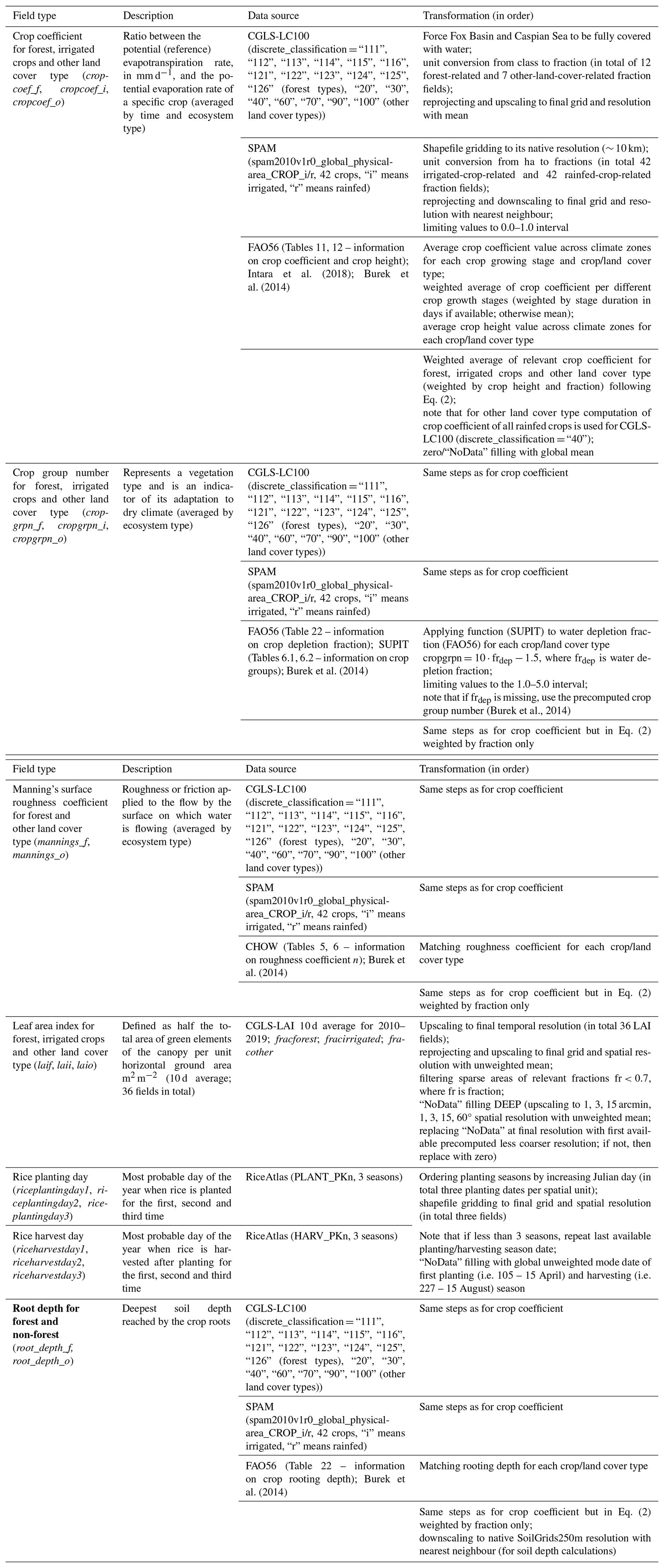
Four steps are involved in generating a particular surface field (see Table 1), with step 3 being the most complex and varied (see Fig. 2 for an example), and step 4 being necessary only for some model specifications (here as required by LISFLOOD; see Table 2).

All techniques applied (see Table 1) to generate CEMS_SurfaceFields_2022 are reproducible to different input data and/or for different output data specifications. Further details on specific manipulations associated with each field category are given in sections below as relevant. Each section has a table with exact data source used per surface field and a step-by-step description of transformations applied to the data to compute the final fields included in CEMS_SurfaceFields_2022 (full technical descriptions for all fields are explained in the LISFLOOD user guide, available online: https://ec-jrc.github.io/lisflood-code/4_Static-Maps-introduction/, last access: 18 June 2024). Although the specific requirements for the dataset were defined by LISFLOOD for the EFAS and GloFAS implementations, summarised in Table 2, they are consistent with requirements of any other environmental models. Regional examples of a sub-set of CEMS_SurfaceFields_2022 are provided to show the level of detail available at each resolution and field and to emphasise the consistency in all the fields, a critical requirement for environment modelling and analysis. Examples focus on three regions of the world: the Po River (Europe), the Amazon River (South America) and the Brahmaputra river (Asia), with additional examples provided in Appendix D.

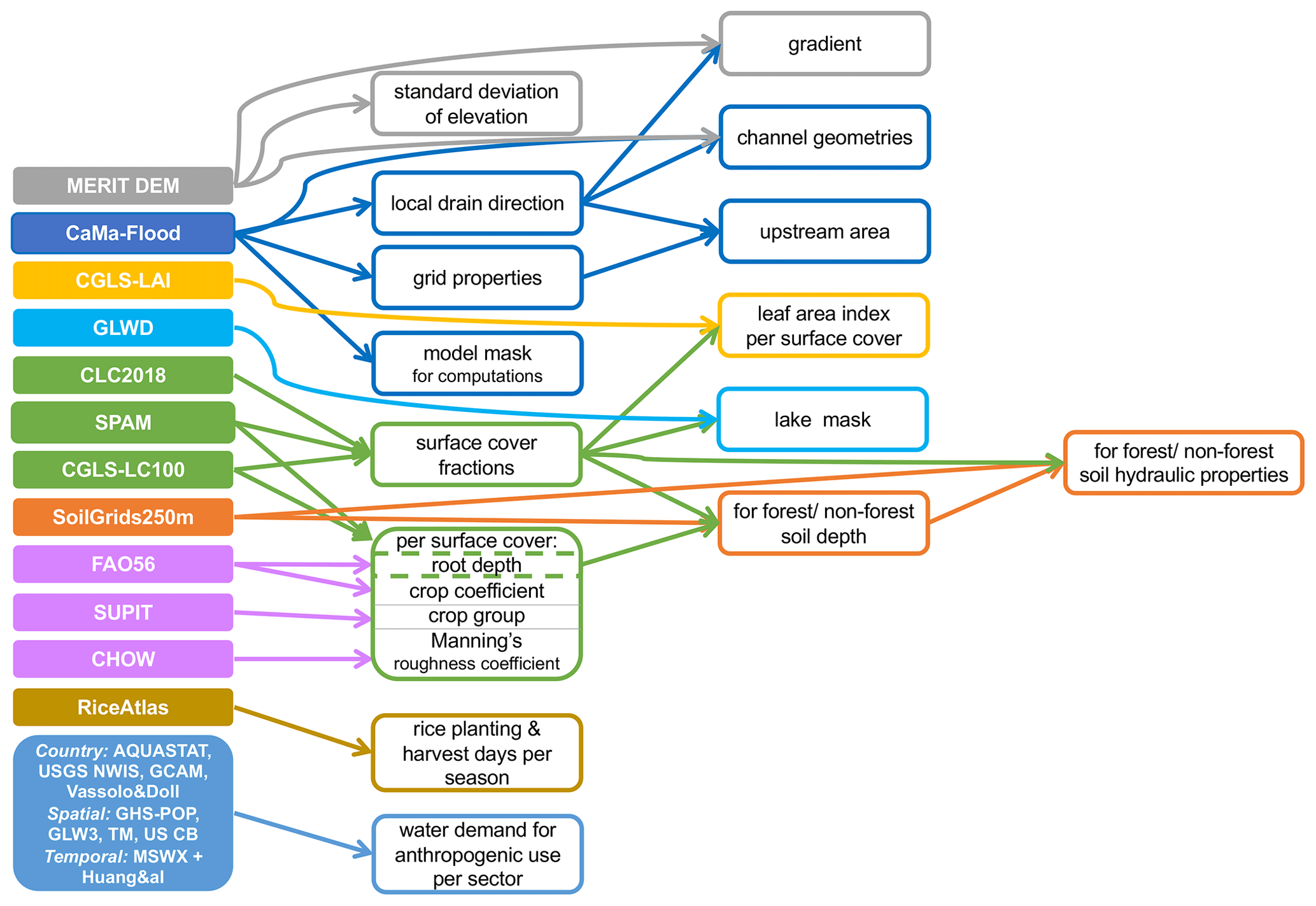
Figure 1 Flow chart connecting input datasets and surface fields created. A dashed border denotes intermediate fields that are not part of the final dataset catalogue.

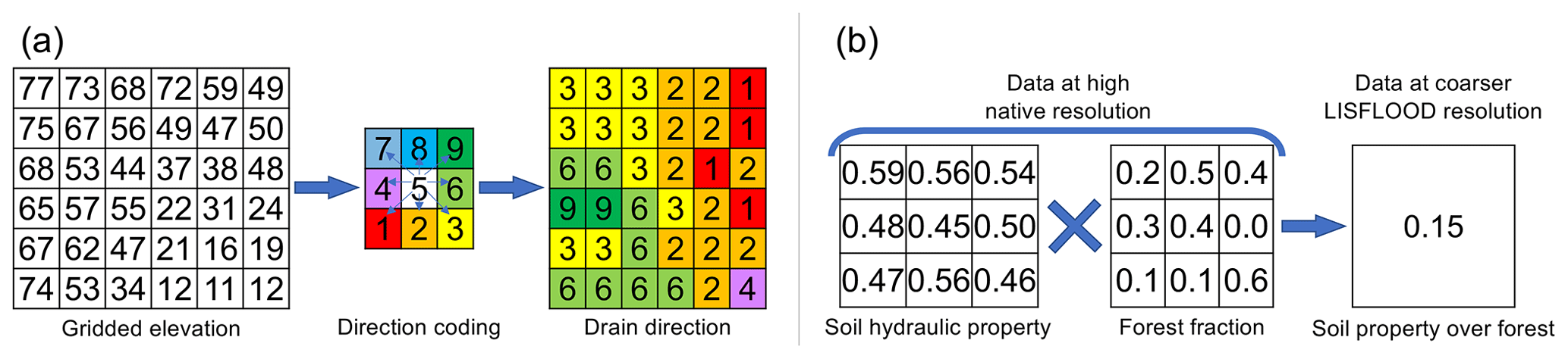
Figure 2 Examples of data manipulation for (left column, panel a) transformation of elevation data into LDD (done within CaMa-Flood) and (right column, panel b) upscaling with weighted average for one final grid cell of soil hydraulic property over forested area.

Table 1 The four steps of a particular surface field generation and associated data manipulations.

Table 2 Dataset files technical specifications.

3 Catchment morphology and river network

3.1 General information

Morphology and channel shape information is essential for the computation of snow melting, temperature scaling and river routing. Alternatively, standard deviation of elevation and other orographic sub-grid parameters are critical for radiation parameterisation, especially for the shadowing effect. Channel geometry fields are needed to describe overbank inundation and infer inundated areas in wetland methane and soil carbon modelling. Land morphology is derived from elevation, and its variability within a single cell can be represented through slope, standard deviation, aspect, etc. River drainage information, derived from elevation, is used to connect the model cells according to the direction of the surface runoff, with channel geometry information used for routing processes.

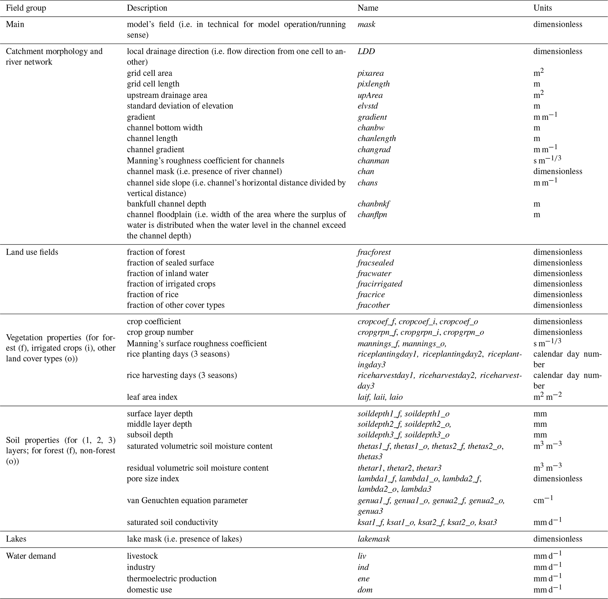
The dataset contains 14 morphology and river network variables (names in brackets in italics correspond to the field names in the data repository).

• Morphologic information: local drainage direction (i.e. flow direction from one cell to another; LDD, dimensionless), upstream drainage area (upArea, m²), grid cell area (pixarea, m²), grid cell length (pixlength, m), standard deviation of elevation (elvstd, m), gradient (i.e. elevation gradient; gradient, m m⁻¹);

• Kinematic wave equation for routing: channel bottom width (chanbw, m), channel length (chanlength, m), channel gradient (changrad, m m⁻¹), Manning's roughness coefficient for channels (chanman, s m${}^{-\mathrm{1}/\mathrm{3}}$);

• River network information: channel mask (i.e. presence of river channel; chan, dimensionless), channel side slope (i.e. channel's horizontal distance divided by vertical distance; chans, m m⁻¹);

• Open water evaporation: bankfull channel depth (chanbnkf, m), channel flood plain (i.e. width of the area where the surplus of water is distributed when the water level in the channel exceeds the channel depth; chanflpn, m).

3.2 Reference data and methodology

Environmental models require an accurate description of terrain and hydro-morphology to represent the hydrodynamics at the spatial resolution of the model. Here all catchment morphology and river network fields are derived from (i) the Catchment-based Macro-scale Floodplain (CaMa-Flood) Global River Hydrodynamics Model v4.0 maps (further referred to as CaMa-Flood) and (ii) the MERIT DEM: Multi-Error-Removed Improved-Terrain digital elevation model v.1.0.3 (further referred to as MERIT DEM). For reference data details, see Appendix A. All fields follow a complex sequential workflow (see Fig. 3 and Table 3). Note that whilst some river network fields were already directly available from the CaMa-Flood catalogue (e.g. LDD, channel length), they had to be adapted to the specific requirements of LISFLOOD. Fields also had to be specifically consistent with an interconnected river network described by the D8 algorithm (O'Callaghan and Mark, 1984; Fig. 2a) which is different to that used by the CaMa-Flood algorithm.

Figure 3 Workflow of complex manipulations to create some of the morphology and river network fields; solid arrows indicate a function transformation, whereas dashed arrows indicate modification of existing input data to LISFLOOD specifications.

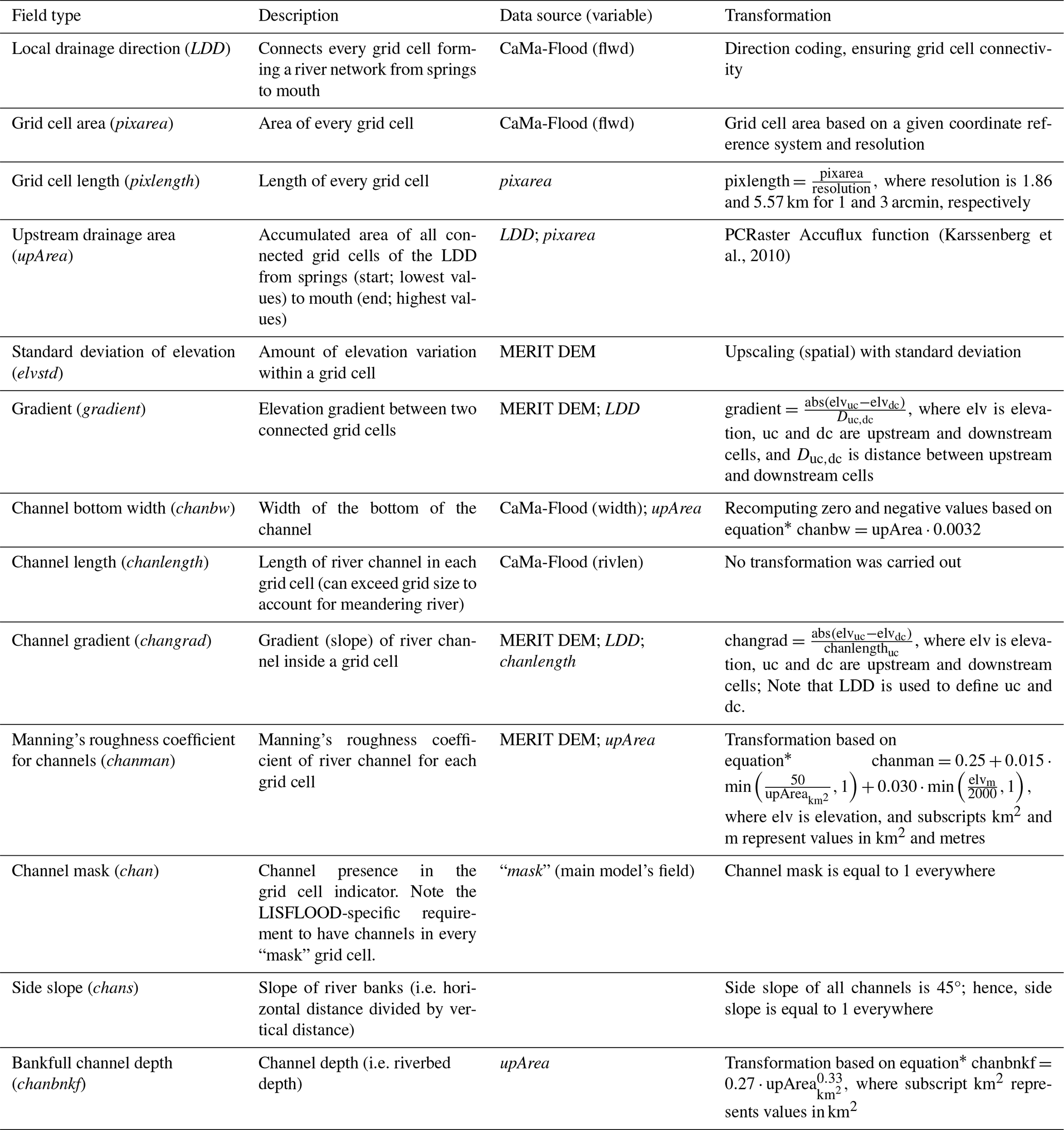
Table 3 Morphology and river network fields, their description, data source and applied transformation; ^* denotes transformation following Burek et al. (2014); name in brackets in italics next to each field corresponds to the name in the data repository.

3.3 Regional examples

Most fields in the catchment morphology and river network category are quite technical and hard to interpret. The ones that can be easily digested are upstream area and standard deviation of elevation, which are presented in Fig. 4 for the Po River area at 1 and 3 arcmin resolutions and in Fig. 5 for the Amazon River and Brahmaputra river areas at 3 arcmin resolution. The field of standard deviation of elevation shows high level of detail over the Brahmaputra river and the benefit of the high-resolution dataset is clearly seen over the Po River.

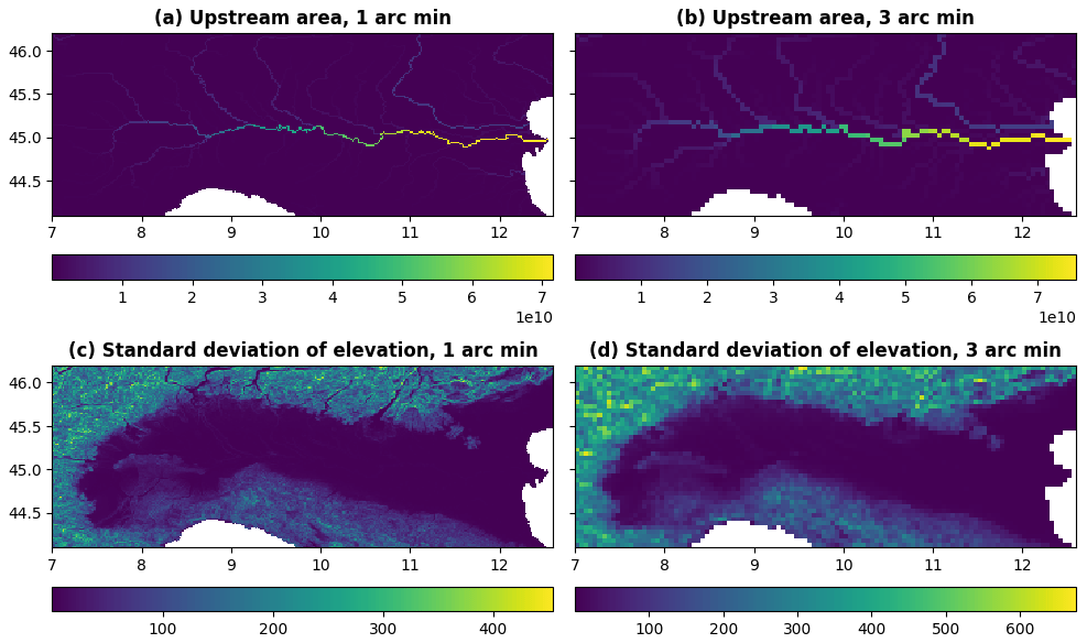
Figure 4 Upstream drainage area in square metres (upper row, panels a and b) and standard deviation of elevation in metres (lower row, panels c and d) at 1 arcmin (∼ 1.9 km at the Equator, left column, panels a and c) and 3 arcmin (∼ 5.6 km at the Equator, right column, panels b and d) resolution for the Po River area in Italy.

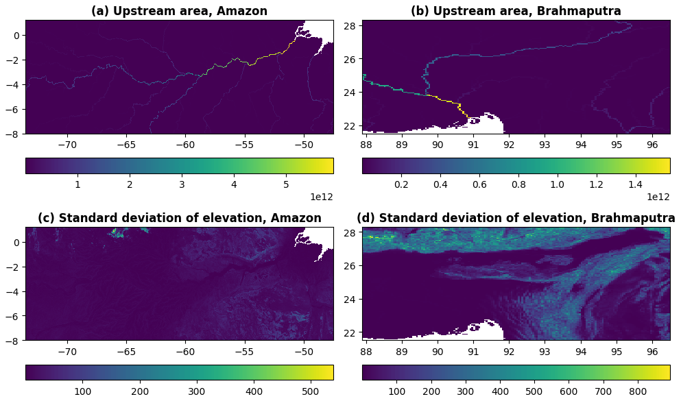
Figure 5 Upstream drainage area in square metres (upper row, panels a and b) and standard deviation of elevation in metres (lower row, panels c and d) at 3 arcmin (∼ 5.6 km at the Equator) resolution for the Amazon River area (left column, panels a and c) and Brahmaputra river area (right column, panels b and d).

4 Land use fields

4.1 General information

Land use is an essential component of environmental models. Many models use a sub-grid cell approach where a single grid cell can include several different land uses with each land use being subject to different prominent physical processes. This approach allows us to keep a high level of accuracy when representing how different types of land cover affect (Balsamo, 2013), for example, the hydrological cycle (e.g. evaporation is different in urban areas compared to forests) while limiting the increase in computational time. Application of land surface fractions includes grid-cell-weighted average skin temperature calculations, biogenic flux calculations, urban planning and climate mitigation plan preparation. For example, sealed surface fraction is necessary for carbon budget calculations and trace gas emissions in general, more explicitly for anthropogenic and residential emission calculations. Irrigated crop and irrigated rice fractions (combined with rice planting and harvesting days) are useful for crop yield and methane emissions modelling.

The dataset differentiates between six different land uses (names in brackets in italics correspond to the field names in the data repository):

• Forest: areas where the main hydrological processes are canopy interception, evapotranspiration from canopies, canopies drainage and evapotranspiration, root uptake, and evaporation from the soil (fraction of forest; fracforest, dimensionless fraction);

• Sealed surface: impervious areas where there is no water infiltration into the soil; that is, water is accumulated in the surface depression, yet evaporates. Once the depression is full, water is transported by a surface runoff (fraction of sealed surface; fracsealed, dimensionless fraction);

• Inland water: open water bodies where the most prominent hydrological process is evaporation (fraction of inland water; fracwater, dimensionless fraction);

• Irrigated crops: areas used by agriculture – water is abstracted from ground water and surface water bodies to irrigate the fields. The main hydrological processes connected with the irrigated crops are canopy interception, evapotranspiration from canopies, canopies drainage and evapotranspiration, root uptake, and evaporation from the soil (fraction of all irrigated crops, excluding rice; fracirrigated, dimensionless fraction);

• Irrigated rice: areas used to grow rice with the flooded irrigation agricultural technique, when water is abstracted from the inland water bodies and delivered to the rice fields. The main hydrological processes connected with rice fields are soil saturation, flooding, rice-growing phase, and soil drainage phase (fraction of irrigated rice; fracrice, dimensionless fraction);

• Other land cover: used in canopy interception, evaporation from the canopies, canopy drainage, plant evapotranspiration and evaporation from the soil hydrological processes. The relative importance of these processes depends on the LAI (fraction of other cover types; fracother, dimensionless fraction).

4.2 Reference data and methodology

In models explicitly accounting for sub-grid variability, the fraction of each land use in every cell must be provided so that process representation for each land use can be weighted accordingly. Here, the majority of land use fields are derived from the Copernicus Global Land Service (CGLS) Land Cover (LC) 100 m map (further referred to as CGLS-LC100). Irrigated crops and irrigated rice fractions are derived from (i) the Spatial Production Allocation Model (SPAM), Global Spatially-Disaggregated Crop Production Statistics Data for 2010 v2.0 (further referred to as SPAM2010) and (ii) the Coordination of Information on the Environment (CORINE) Land Cover (CLC) inventory for 2018 (further referred to as CLC2018). For reference data details, see Appendix A. The derivation of fractions of the five land use classes used in LISFLOOD (and additional ocean fraction for consistency check) follows specific steps (see Fig. 6) summarised in Table 4. Note that LISFLOOD requires all “mask” (main model's field) grid cells to have at least one non-zero fraction type. Hence, the extra step in the generation of the inland water fraction field was to set empty grid cells (i.e. grid cells that based on the data source are fully covered with ocean) as fully covered with inland water.

Figure 6 Workflow of complex manipulations to create land use fields; solid arrows indicate a function transformation, whereas dotted arrows indicate upscaling; dashed boxes indicate the intermediate fields used for other field generation.

Table 4 Fraction of land use fields, their description, data source and applied transformations; “sum” refers to the sum of all fractions except “other land cover fraction”; cells with bold font show required intermediate fields; name in brackets in italics next to each field corresponds to the name in the data repository.

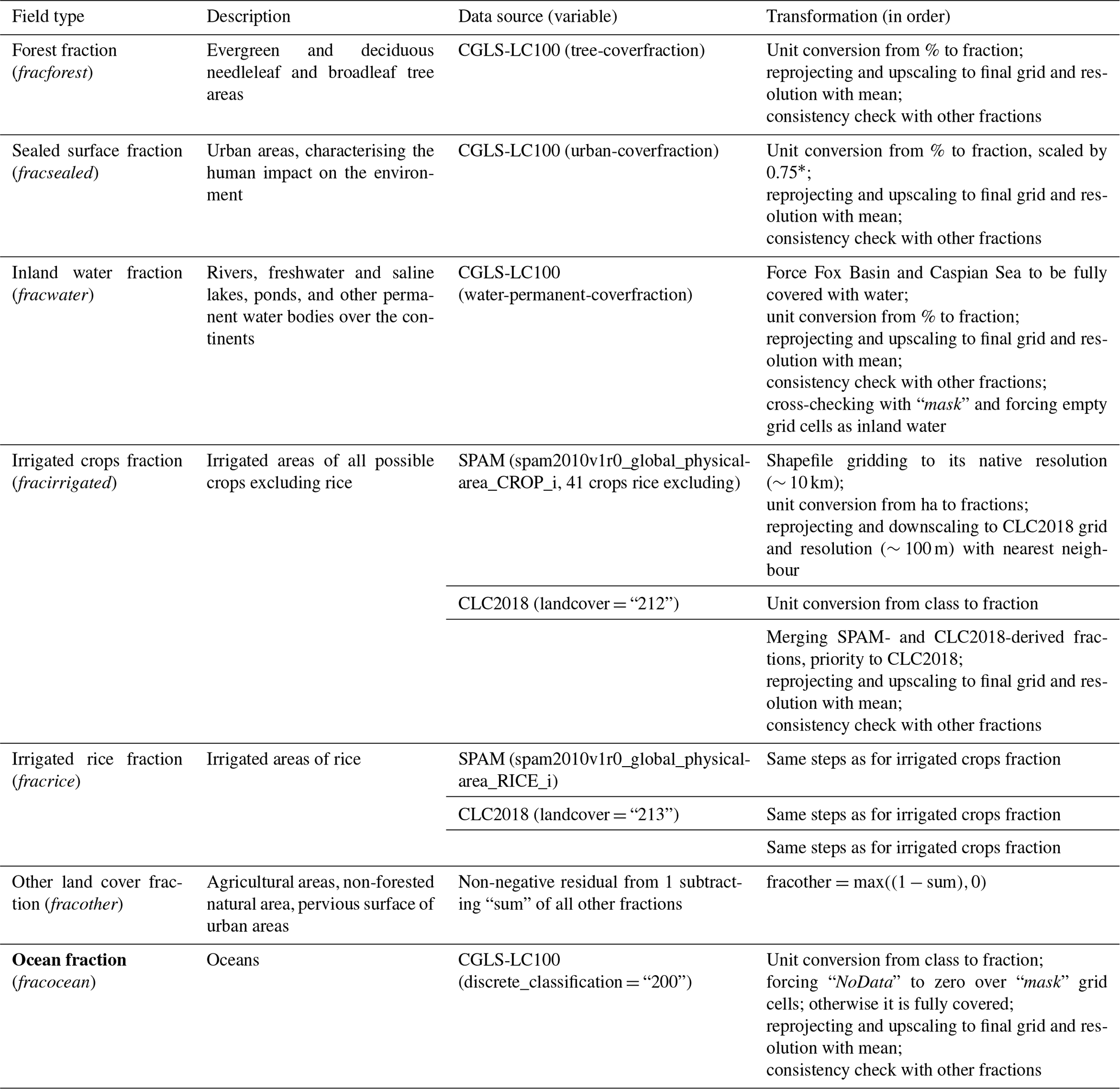
^* For the sealed surface fraction, it is assumed that water can infiltrate in roughly 25 % of urban areas at kilometre scale through, for example, trees along the road, bushes along the fence, and grass or moss between concrete tiles or cobblestones.

To ensure consistency between fractions, the sum of all fraction fields must be 1 at any resolution. When the sum is greater than 1, the inland water fraction value is assumed correct (input data corrected prior computation over Fox Basin and Caspian Sea), and all other fractions are corrected (fracXX) following Eq. (1):

$$\begin{array}{}\text{(1)}& \begin{array}{rl}& \mathrm{fracXX}\\ & ={\mathrm{fracXX}}_{\mathrm{raw}}\left(\mathrm{1}-{\displaystyle \frac{\begin{array}{c}{\mathrm{fracwater}}_{\mathrm{raw}}+{\mathrm{fracocean}}_{\mathrm{raw}}+{\mathrm{fracforest}}_{\mathrm{raw}}+{\mathrm{fracsealed}}_{\mathrm{raw}}\\ +{\mathrm{fracirrigated}}_{\mathrm{raw}}+{\mathrm{fracrice}}_{\mathrm{raw}}-\mathrm{1}\end{array}}{\begin{array}{c}{\mathrm{fracforest}}_{\mathrm{raw}}+{\mathrm{fracsealed}}_{\mathrm{raw}}\\ +{\mathrm{fracirrigated}}_{\mathrm{raw}}+{\mathrm{fracrice}}_{\mathrm{raw}}\end{array}}}\right),\end{array}\end{array}$$

where raw refers to the original (i.e. before consistency check) fraction of XX which can be the forest, irrigated crops, rice or sealed surfaces.

The generated fraction fields, e.g. forest (see Fig. 7a) and other land cover (see Fig. 7b), have generally good consistency with other up-to-date products like ESA CCI Land Cover time series v2.0.7 (ESA CCI map viewer https://maps.elie.ucl.ac.be/CCI/viewer/, last access: 18 June 2024; Defourny et al., 2017).

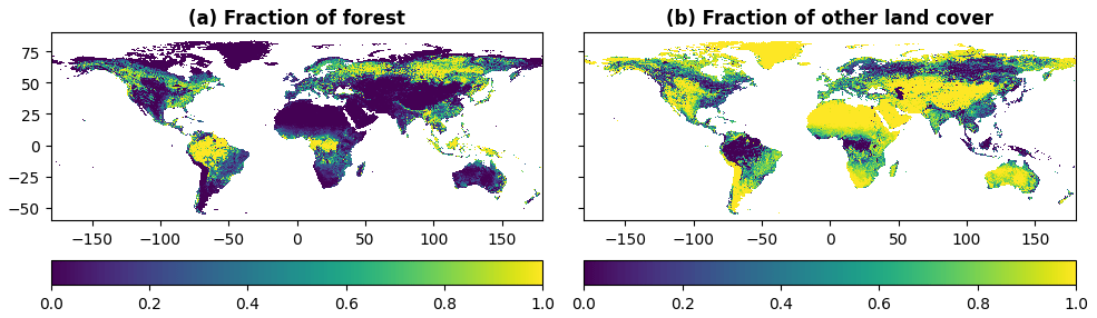
Figure 7 Fraction of forest (left column, panel a) and fraction of other land cover (right column, panel b) at 3 arcmin (∼ 5.6 km at the Equator) resolution for the global region.

4.3 Regional examples

All fields in the land use category are easy to interpret as they represent the fraction of grid cell covered by one or another surface cover type. The most interesting ones are fraction of forest, fraction of inland water, fraction of irrigated crops and fraction of rice. These fractions are presented in Fig. 8 for the Po River area at 1 and 3 arcmin resolutions and in Fig. 9 for the Amazon River and Brahmaputra river areas at 3 arcmin resolution. Figures show a high level of detail visible for the fields of fraction of forest and fraction of inland water (e.g. Amazon River), especially at the highest spatial resolution (Po River).

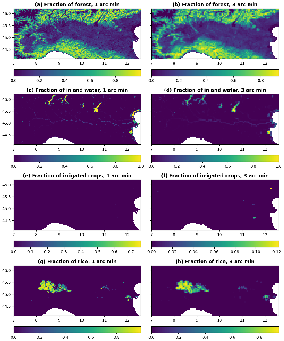
Figure 8 Fraction of forest (upper row, panels a and b), fraction of inland water (second row, panels c and d), fraction of irrigated crops (third row, panels e and f) and fraction of rice (lower row, panels g and h) at 1 arcmin (∼ 1.9 km at the Equator, left column, panels a, c, e and g) and 3 arcmin (∼ 5.6 km at the Equator, right column, panels b, d, f and h) resolution for the Po River area in Italy.

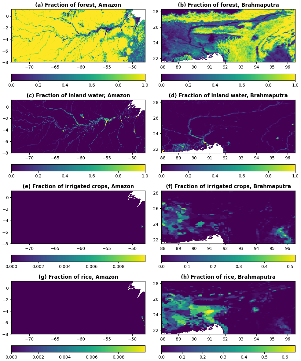
Figure 9 Fraction of forest (upper row, panels a and b), fraction of inland water (second row, panels c and d), fraction of irrigated crops (third row, panels e and f) and fraction of rice (lower row, panels g and f) at 3 arcmin (∼ 5.6 km at the Equator) resolution for the Amazon River area (left column, panels a, c, e and g) and Brahmaputra river area (right column, panels b, d, f and h).

5 Vegetation properties

5.1 General information

Vegetation-related information contributes to the computation of precipitation interception, evaporation, transpiration, and root water uptake. Depending on the model, vegetation dynamics can be represented with different degrees of complexity including in hydrology processes, vegetation growth and feedback on climate (Bonan et al., 2003). For rice, being the world's most important food crop and having specific water demands, its water cycle is often considered explicitly. Rice planting and harvesting dates, being critical information to represent the inter-annual variability in its water demand, provided the maximum of three growing seasons. The variables allow us to model how vegetation affects the hydrology, with a particular focus on root water uptake and transpiration depending on vegetation type and vegetation state (e.g. water stress conditions). For example, the crop group number depends on the critical amount of soil moisture below which water uptake from plants is reduced as they start closing their stomata. Alternative use of fields such as the leaf area index (LAI) includes biomass allocation, which can be used for fire danger forecasting and carbon stock monitoring. Rice planting/harvesting days are important for the yearly cycle of methane modelling.

The dataset describes vegetation properties through four variables (note that LAI consists in total of thirty-six 10 d average fields) for each of forest (_f), irrigated crops (_i), and other land cover types (_o) and another six (two types times three seasons) variables for rice (names in brackets in italics correspond to the field names in the data repository):

• Transpiration rate: crop coefficient (cropcoef_f, cropcoef_i, cropcoef_o, dimensionless);

• Water uptake: crop group number (cropgrpn_f, cropgrpn_i, cropgrpn_o, dimensionless);

• Surface runoff generation and water routing: Manning's surface roughness coefficient (mannings_f, mannings_o, s m${}^{-\mathrm{1}/\mathrm{3}}$), rice planting and harvesting days (riceplantingday1, riceplantingday2, riceplantingday3, calendar day number; riceharvestday1, riceharvestday2, riceharvestday3, calendar day number);

• Water interception and evaporation: leaf area index (laif, laii, laio, m² m⁻²).

5.2 Reference data and methodology

In addition to the land use fraction, the distribution of vegetation type and characteristics is required to capture the difference in environmental processes, such as water intake of evaporation. Here the vegetation properties are derived from many data sources using maps to account for the species spatial distribution (i.e. CGLS-LC100 and SPAM2010) and tables to obtain associated hydro-dynamics properties for crops, e.g. (i) the Food and Agriculture Organisation (FAO) of the United Nations Irrigation and Drainage Paper No. 56 (further referred to as FAO56), (ii) the WOFOST 6.0 crop simulation model description (further referred to as SUPIT), and (iii) for river hydraulics the Open-Channel Hydraulics manual (further referred to as CHOW). Time evolution of vegetation is based on the Copernicus Global Land Service (CGLS) Leaf Area Index (LAI) 1 km Version 2 collection (further referred to as CGLS-LAI); time evolution of crops is based on the RiceAtlas v3 (further referred to as RiceAtlas). For reference data details, see Appendix A. This requires assumptions to be made in case different sources do not contain the same information and transformations need to be applied, depending on the vegetation type. The main data sources and general transformation steps (see Fig. 10) to derive the 18 vegetation property fields are summarised in Table 5 and the following text. Note that the “crop group number” variable corresponds to a water depletion value and can be averaged across different crop types.

Figure 10 Workflow of complex manipulations to create some of the vegetation property fields, e.g. crop coefficient (left column, upper row, panel a), Manning's surface roughness coefficient (right column, upper row, panel b), crop group number (left column, lower row, panel c), and root depth (right column, lower row, panel d); solid arrows indicate a function transformation, whereas dotted arrows indicate upscaling; dashed boxes indicate the intermediate fields used for other field generation, whereas dotted boxes indicate the fields only used for the vegetation-related fields.

Table 5 Vegetation property fields, their description, data source and applied transformations; cells with bold font show required intermediate fields; name in brackets in italics next to each field corresponds to the name in the data repository.

The final step of the crop coefficient; crop group number; Manning's surface roughness coefficient; and additional crop height (for crop coefficient calculation) and root depth (for soil depth calculation, see Sect. 6.2) for forest, irrigated, crops, and other land cover types is to compute weighted averages of their components (e.g. different forest types) following Eq. (2):

$$\begin{array}{}\text{(2)}& K={\displaystyle \frac{A_{\mathrm{1}}\cdot f{r}_{\mathrm{1}}\cdot K_{\mathrm{1}}+A_{\mathrm{2}}\cdot f{r}_{\mathrm{2}}\cdot K_{\mathrm{2}}+\mathrm{\dots }+A_N\cdot f{r}_N\cdot K_N}{A_{\mathrm{1}}\cdot f{r}_{\mathrm{1}}+A_{\mathrm{2}}\cdot f{r}_{\mathrm{2}}+\mathrm{\dots }+A_N\cdot f{r}_N}},\end{array}$$

where A is a scaling parameter (equals 1, except for crop coefficient where it equals to crop height); fr refers to the fraction of crop or land cover type; K refers to the default (i.e. source-table-based) variable in question, values 1 … N represent the number of crop or land cover types included in the field (i.e. N= 12 for forest, N= 41 for irrigated crops, N= 7 for other land cover types; for CGLS-LC100-type “40” (cropland), default values are based on 42 rainfed crops).

The generated vegetation property fields, e.g. crop coefficient for forest (see Fig. 11a) and other land covers (see Fig. 11b), follow the main features of, for example, generated forest fraction.

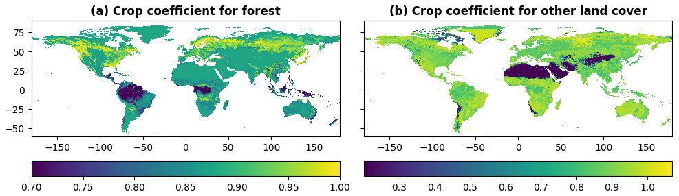
Figure 11 Crop coefficient for forest (left column, panel a) and crop coefficient for other land cover types (right column, panel b) at 3 arcmin (∼ 5.6 km at the Equator) resolution for the global region.

5.3 Regional examples

All fields in the vegetation properties category are complementary to the land use fractions and help to understand for example the difference in evaporation water intake. The fields easiest to interpret are the crop coefficient and the crop group number, which are presented for forest in Fig. 12 for the Po River area at 1 and 3 arcmin resolutions and in Fig. 13 for the Amazon River and Brahmaputra river areas at 3 arcmin resolution. For example, fields of crop group number for forest (i.e. different forest types) show a transition of vegetation resilience towards dry conditions in the Brahmaputra river area.

Figure 12 Crop coefficient for forest (upper row, panels a and b) and crop group number for forest (lower row, panels c and d) at 1 arcmin (∼ 1.9 km at the Equator, left column, panels a and c) and 3 arcmin (∼ 5.6 km at the Equator, right column, panels b and d) resolutions for the Po River area in Italy.

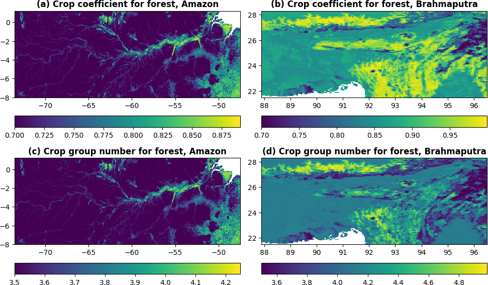
Figure 13 Crop coefficient for forest (upper row, panels a and b) and crop group number for forest (lower row, panels c and d) at 3 arcmin (∼ 5.6 km at the Equator) resolution for the Amazon River area (left column, panels a and c) and Brahmaputra river area (right column, panels b and d).

6 Soil properties

6.1 General information

In land surface and distributed hydrological models, the water movement, storage and uptake from the soil are often described by the soil water retention curve (SWRC). The SWRC is derived empirically by measuring how water is retained and released by different soil types. Throughout time, different SWRCs have been developed and integrated into models. The most widely applied SWRCs are from Brooks and Corey (Brooks and Corey, 1964), Fredlund and Xing (Fredlund and Xing, 1994), van Genuchten (van Genuchten, 1980), and Gardner (Gardner, 1956). Different SWRC equations require different parameters, some shared between different SWRC concepts, e.g. referring to physical soil characteristics such as water saturated and unsaturated content, hydraulic conductivity and pore size, while others are uniquely describing the SWRC function shape and not directly related to soil properties. Often, for computational reasons, the soil profile from ground level to bedrock depth is sliced into layers, at the modeller's choice, and the SWRC function is applied to each soil layer. An alternative use of soil properties is for soil moisture calculations.

The dataset includes variables required to apply the van Genuchten SWRC equations (van Genuchten, 1980) to describe the water dynamics through a vertical soil profile composed of three layers (1, 2, 3). Each variable is required for each soil layer and for forest (_f) or non-forest (_o) land uses, with different soil depths in forest (_f) and non-forest (_o) areas, following root depth values from Allen at al. (1998), referred to as FAO56 (total of 29 variables; names in brackets in italics correspond to the field names in the data repository):

• Soil profile: surface layer depth (soildepth1_f, soildepth1_o, mm), middle layer depth (soildepth2_f, soildepth2_o, mm), subsoil depth (soildepth3_f, soildepth3_o, mm);

• Soil hydraulic properties: saturated (thetas1_f, thetas1_o, thetas2_f, thetas2_o, thetas3, m³ m⁻³) and residual (thetar1, thetar2, thetar3, m³ m⁻³) volumetric soil moisture content, pore size index (lambda1_f, lambda1_o, lambda2_f, lambda2_o, lambda3, dimensionless), van Genuchten equation parameter (genua1_f, genua1_o, genua2_f, genua2_o, genua3, cm⁻¹), saturated soil conductivity (ksat1_f, ksat1_o, ksat2_f, ksat2_o, ksat3, mm d⁻¹).

6.2 Reference data and methodology

Soil proprieties are derived from the International Soil Reference and Information Centre (ISRIC) SoilGrids250m global gridded soil information release 2017 (further referred to as SoilGrids250m). For reference data details, see Appendix A. Soil proprieties are computed for both forested and non-forested (also known in literature as “others”) areas, expressed as fractions (main source is forest fraction based on CGLS-LC100; see Section 4.2), where non-forested area is the complementary fraction of forest. Soil depth layers are derived first and used as input to the soil hydraulic equations used to derive the properties, following a sequential workflow (see Fig. 14 and Table 6). Equations used are from Tóth et al. (2015).

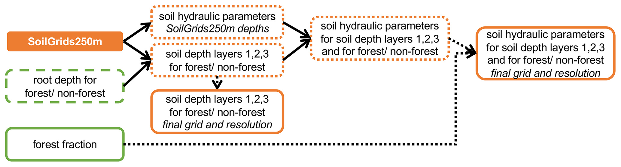
Figure 14 Workflow to generate the soil-related fields; solid arrows indicate a function transformation, whereas dotted arrows indicate upscaling; dashed boxes indicate the intermediate fields used for other field generation, whereas dotted boxes indicate the fields only used for the soil-related fields; “SoilGrids250m depths” represents fields at the SoilGrids250m native grid and resolution with six default depths, “final grid and resolution” represents fields at the dataset's final grid and resolution; boxes with no explicit indication represent fields at SoilGrids250m native grid and resolution only.

Table 6 Soil property fields, their description and applied transformations; name in brackets in italics next to each field corresponds to the name in the data repository.

Two of the most common soil parameters of land surface and hydrological models, saturated hydraulic conductivity (ksat) and saturated water content, are shown in Fig. 15.

Saturated hydraulic conductivity (ksat; see Fig. 15a) ranges from 2 to 7445 mm d⁻¹. The highest ksat values are concentrated in desert areas such as the Sahara, Arabian Peninsula, Gobi, Patagonian, Sonoran–Mojave, and Kalahari and Namib deserts. Low ksat values between 2 and 18 mm d⁻¹ are found in the Amazon river basin, the lower Mississippi River basin and South East Asia; ksat was visually compared against eight global datasets developed with different input data and/or pedotransfer functions (PTFs) (Zhang and Schaap, 2019; Gupta et al., 2021); a general agreement is noticeable in areas that show low variability across all datasets. Northern Russia, Canada, South East Asia and the Sonoran–Mojave desert are the areas with high variability among datasets, with values ranging from very low to very high ksat. Source of uncertainties in ksat values are primarily due to little availability of soil samples and measurements carried out in those areas. Moreover, the climatic context plays a relevant role in clay mineralogy composition, organic composition and soil pores structure (Hodnett and Tomasella, 2002), which influence how water flows through the soil. Therefore, the PTF developed using soil samples collected in temperate areas (such as Europe) are expected to have a different hydraulic behaviour compared to those collected in tropical climates (Gupta et al., 2021), as also seen in Fig. 15a.

Saturated water content (see Fig. 15b) ranges between 0.27 to 0.79, with 80 % of values between 0.40 and 0.46. A comparison with other global datasets was not carried out; however, uncertainties are expected to be of the same order of magnitude as those of ksat, given the fact that the saturated water content is calculated using bulk density and clay content data.

Figure 15 Saturated soil hydraulic conductivity for forested areas of soil depth layer 2 (in mm d⁻¹) (left column, panel a) and saturated volumetric soil moisture (i.e. water) content for forested areas of soil depth layer 2 (right column, panel b) at 3 arcmin (∼ 5.6 km at the Equator) resolution for the global region.

6.3 Regional examples

The majority of soil property fields are easy to interpret. Saturated soil conductivity, ksat, and saturated volumetric soil moisture content are presented for forested areas of soil depth layer 2 in Fig. 16 for the Po River area at 1 and 3 arcmin resolutions and in Fig. 17 for the Amazon River and the Brahmaputra river areas at 3 arcmin resolution. The field of saturated soil conductivity for forest shows how easy it is for water to penetrate soil, depending on forest type. The field of saturated volumetric soil moisture content shows what is the maximum amount of water that the soil can absorb, depending on forest type. These fields have interesting features over Brahmaputra river area.

Figure 16 Saturated soil hydraulic conductivity for forested areas of soil depth layer 2 (in mm d⁻¹) (upper row, panels a and b) and saturated volumetric soil moisture (i.e. water) content for forested areas of soil depth layer 2 (lower row, panels c and d) at 1 arcmin (∼ 1.9 km at the Equator, left column, panels a and c) and 3 arcmin (∼ 5.6 km at the Equator, right column, panels b and d) resolution for the Po River area in Italy.

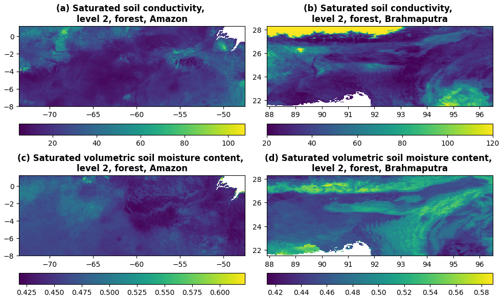
Figure 17 Saturated soil hydraulic conductivity for forested areas of soil depth layer 2 (in mm d⁻¹) (upper row, panels a and b) and saturated volumetric soil moisture (i.e. water) content for forested areas of soil depth layer 2 (lower row, panels c and d) at 3 arcmin (∼ 5.6 km at the Equator) resolution for the Amazon River area (left column, panels a and c) and Brahmaputra river area (right column, panels b and d).

7 Lakes

7.1 General information

Lakes (and reservoirs) are important as they influence river discharge variability but also the atmosphere regionally and globally. The area covered by lakes can be used for computing evaporation from open water, freshwater storage, unregulated surface water extent, fresh water scarcity indexes and biogenic greenhouse gas emission, as well as for reproducing different climate mitigation scenarios. The CEMS_SurfaceFields_2022 dataset only includes data on lake extent and not reservoirs (generally smaller). Lake mask describes the presence of lakes and is consistent with fraction of inland water. The field's name in the data repository is lakemask, dimensionless.

7.2 Reference data and methodology

The lake mask field is derived from the Global Lakes and Wetlands Database (further referred to as GLWD). For reference data details, see Appendix A; for workflow, see Table 7.

Table 7 Lake field, its description, data source and transformation; name in brackets in italics next to the lake field corresponds to the name in the data repository.

7.3 Regional examples

The lake mask field is easy to interpret as it shows which grid cells from fraction of inland water field have lakes. The lake mask field is presented in Fig. 18 for the Po River area at 1 and 3 arcmin resolution, and in Fig. 19 for the Amazon River and Brahmaputra river areas at 3 arcmin resolution. Figures show the abundance of lakes over Amazon River area and detailed lake shapes over Po River area described by the 1 arcmin resolution field.

Figure 18 Lake mask at 1 arcmin (∼ 1.9 km at the Equator, left column, panel a) and 3 arcmin (∼ 5.6 km at the Equator, right column, panel b) resolution for the Po River area in Italy.

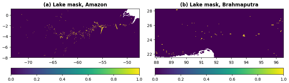
Figure 19 Lake mask at 3 arcmin (∼ 5.6 km at the Equator) resolution for the Amazon River area (left column, panel a) and Brahmaputra river area (right column, panel b).

8 Water demand

8.1 General information

Some environmental models explicitly represent the number of human interventions impacting on the water cycle. One of the most common is water demand, which represents the withdrawal of water from natural water sources (e.g. rivers, reservoirs, groundwater) to satisfy the water demand for anthropogenic use. The segregation of the total water demand for anthropogenic use into four main sectors, namely domestic, energy, industrial and livestock water withdrawal, enables a more accurate representation of the processes and follows the Food and Agriculture Organisation of the United Nations (FAO) terminology (Kohli et al., 2012). Domestic water withdrawal represents indoor and outdoor household water use as well as other uses (e.g. industrial and urban agriculture) connected to the municipal system (e.g. water use by shops, schools and public buildings). Electricity (energy) water withdrawal is the water use for the cooling of thermoelectric and nuclear power plants. Water withdrawal for industry is the water used for fabricating, processing, washing, cooling or transporting products and also includes water within the final products and water used for sanitation within the manufacturing facility. Livestock withdrawal is the demand for drinking and cleaning purposes of livestock.

Higher accuracy in environmental modelling is achieved by differentiating water demand sources and by allocating different levels of priority to different usages. Within LISFLOOD, for instance, water demand for the energy sector and flooded irrigation (rice crops) is supplied by surface water bodies only. Non-flooded irrigation, domestic, industrial and livestock water demands can be supplied by both groundwater and surface water bodies. Moreover, the domestic water demand has the highest priority in case of water scarcity conditions.

It must be noted that the fields of water demand for agriculture are not included in this dataset because LISFLOOD computes crop water demand internally by accounting for climatic conditions, information on land cover (see Sect. 4.2), crops properties (see Sect. 5.2) and soil properties (see Sect. 6.2). Conversely, fields representing the volume of water to satisfy the domestic, energy, industrial and livestock demands must be provided as input. Domestic, industrial, energy and livestock water demand volumes have seasonal (e.g. due to temperature differences) and inter-annual variations (e.g. due to population changes and different economic conditions). In order to account for this variability, in LISFLOOD the four sectoral water demand fields provide daily water demand data with monthly or annual variability from 1 January 1979 to 31 December 2019. The water demand values are provided in millimetres per day (mm d⁻¹), with one field per month (the first day of each month is used as representative timestamp for the entire month) for domestic and energy demand and one value per year (the monthly fields are repeated 12 times per year) for industrial and livestock demand.

Water availability, ecosystem long-term ecological status and anthropogenic needs must be accounted for to evaluate the long-term sustainability of water withdrawals. However, the spatial scales of water use data and available water resources data often do not match due to different ways of data surveying and/or modelling (McManamay et al., 2021; Zhang et al., 2023), and this creates a technical hurdle. Alternative use of the gridded sectoral water demand information is for (i) the statistical analysis of long-term spatiotemporal patterns and trends of water demand, (ii) the evaluation of the long-term sustainability and impacts of water withdrawals (e.g. in connection to remote sensing-derived datasets of surface water extent or groundwater total storage), (iii) the analysis of ecosystem–water–food–energy nexus (Karabulut et al., 2016), (iv) the evaluation of the impacts on water resources of economical and price policies (Dolan et al., 2021), and (v) the analysis of the responses in sectoral water use during hydroclimatic extremes (Belleza et al., 2023).

The CEMS_SurfaceFields_2022 dataset includes water demand for four main sectors (note that each sector consists in total of 12 daily water demand fields per 41 (1979–2019) years, so 492 fields per sector) (names in brackets in italics correspond to the field names in the data repository): livestock (liv, mm d⁻¹), industry (ind, mm d⁻¹), energy production, (ene, mm d⁻¹) and domestic use (dom, mm d⁻¹). The temporal extension of the water demand fields presented in this paper includes the most recent information of water demand at the time of the dataset's preparation. Readers that are interested in using more recent water demand data are invited to follow the protocol presented in Sect. 8.2 to further extend in time the provided fields.

8.2 Reference data and methodology

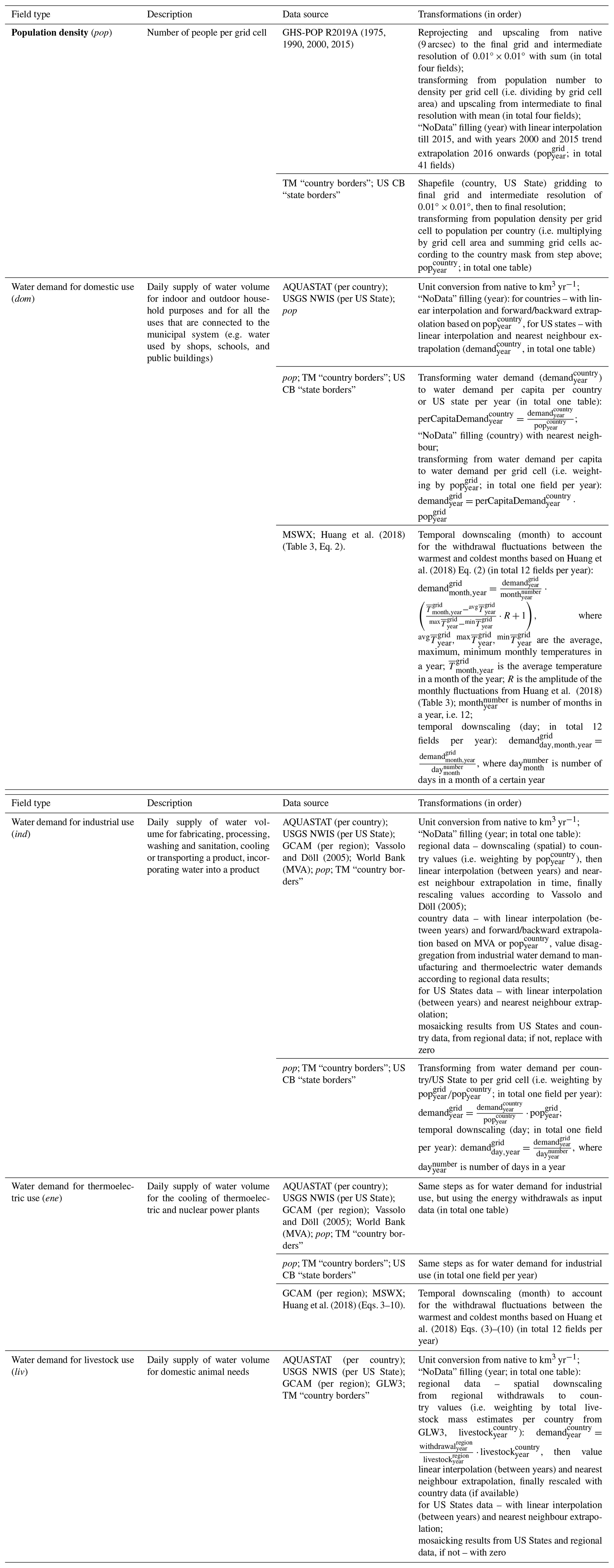
Global gridded water demand fields with monthly variability were generated for the four sectors using the main data sources listed here and following the transformations summarised in Table 8 (for additional information and extra details, see the GitHub repository https://github.com/ec-jrc/lisflood-utilities/tree/master/src/lisfloodutilities/water-demand-historic last access: 18 June 2024): (i) AQUASTAT, (ii) United States Geological Survey National Water Information System (further referred to as USGS NWIS), (iii) Global Change Analysis Model (further referred to as GCAM), (iv) the Gridded Livestock of the World (GLW) version3 (further referred to as GLW3), and (v) the Global Human Settlement Population Grid multitemporal version R2019A (further referred to as GHS-POP). For the full list of reference data and details, see Appendix A.

The water demand values are provided in mm d⁻¹ and one field per month from 1 January 1979 to 31 December 2019 (the first day of each month is used as the representative timestamp for the entire month). The methodology applied largely follows Huang et al. (2018), with the key differences being the use of freely available datasets and the higher resolution of the resulting fields. Spatial downscaling was achieved following the approach by Hejazi et al. (2014); temporal downscaling was performed following the approaches by Wada et al. (2011), Voisin et al. (2013) and Huang et al. (2018). It should be noted that country-scale estimates (from AQUASTAT) were integrated with state-level water withdrawal estimates (from USGS NWIS). The protocol for the integration of local information with global data sources was developed for further use in the future to enable the integration of other regional or national datasets as soon as they become available.

Table 8 Water demand fields, their description, data source and applied transformations; cells with bold font show required intermediate fields; name in brackets in italics next to each field corresponds to the name in the data repository.

To the best of the authors' knowledge, no other publicly accessible temporally varying global water demand field set exists (only static datasets). A rigorous validation of the temporally varying water demand fields is not straightforward at the global scale, as the only comprehensive global data source, FAO AQUASTAT, was used to create the fields.

8.3 Regional examples

In general, fields in the water demand category are easy to interpret as they show how much water per day is needed to satisfy certain types of human-induced needs. In reality, water demand fields are mainly covering urbanised areas and are scattered around (i.e. not continuously looking field), with relatively small variations in field values from month to month. An example for domestic water use is presented for August 2018 in Fig. 20 for the Po River area at 1 and 3 arcmin resolutions and in Fig. 21 for the Amazon River and Brahmaputra river areas at 3 arcmin resolution.

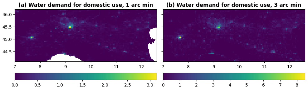
Figure 20 Water demand for domestic use in mm d⁻¹ at 1 arcmin (∼ 1.9 km at the Equator, left column, panel a) and 3 arcmin (∼ 5.6 km at the Equator, right column, panel b) resolution for the Po River area in Italy.

Figure 21 Water demand for domestic use in mm d⁻¹ at 3 arcmin (∼ 5.6 km at the Equator) resolution for the Amazon River area (left column, panel a) and Brahmaputra river area (right column, panel b).

9 Data, access, licensing and documentation

CEMS_SurfaceFields_2022 is an open-source dataset of the Copernicus Emergency Management Service describing key components of the Earth surface generally required in environmental and hydrological modelling, including Earth system modelling and numerical weather prediction. The dataset includes static fields (e.g. forest fraction), yearly cycle fields (e.g. 10 d average LAI, in total 36 fields) and yearly varying fields (e.g. water demand). The surface fields are based on 25 different sources, including global and regional high-resolution (up to 100 m) gridded and vector datasets. They were processed into two sets of fields (i) at 1 arcmin resolution (∼ 1.86 km at the Equator) over Europe (72.25° N/22.75° N, 25.25° W/50.25° E; 4530×2970 grid cells) and (ii) at 3 arcmin resolution (∼ 5.57 km at the Equator) over the globe (90.00° N/90.00° S, 180.00° W/180.00° E; 7200×3600 grid cells) to provide an up-to-date surface state for six main field groups: (1) catchment morphology and river network, (2) land use fields, (3) vegetation properties, (4) soil properties, (5) lakes and (6) water demand.

The CEMS_SurfaceFields_2022 dataset consists, in total, of 140 gridded fields at EPSG:4326 – WGS84: World Geodetic System projection in NetCDF format with information on Earth's surface state (see Table 9 for the full list of fields), which are grouped thematically into sub-folders. The 1 arcmin European fields have a total memory storage volume of 9.3 GB, and the 3 arcmin global fields have a total volume of 22.7 GB. The CEMS_SurfaceFields_2022 dataset is freely available for download from the Joint Research Centre (JRC) Data Catalogue (https://data.jrc.ec.europa.eu/, last access: 18 June 2024). The set of global surface fields at 3 arcmin resolution can be found here (JRC Data Catalogue – LISFLOOD static and parameter maps for GloFAS – European Commission (europa.eu), https://data.jrc.ec.europa.eu/dataset/68050d73-9c06-499c-a441-dc5053cb0c86, last access: 18 June 2024), and the set of surface fields for the European domain at 1 arcmin resolution can be found here (JRC Data Catalogue – LISFLOOD static and parameter maps for Europe – European Commission (europa.eu), https://data.jrc.ec.europa.eu/dataset, last access: 18 June 2024). The README.txt file that can be found there contains the basic description of each surface field, including general information, data description, file overview, methodological information, and data access and sharing information. For a detailed technical description of how the surface fields were generated, refer to the LISFLOOD user guide, available online: https://ec-jrc.github.io/lisflood-code/4_Static-Maps-introduction/, last access: 18 June 2024. The changelog.txt file provides users with information on updates to the datasets. The copyright.txt file provides information about the data licence (CC BY 4.0).

Table 9 Full list of surface fields with short description and units included in CEMS_SurfaceFields_2022 dataset; name in italics corresponds to the field's file name in the data repository.

Whilst the CEMS_SurfaceFields_2022 dataset followed the strict requirements of the LISFLOOD-OS model (e.g. format, treatment of missing values, number of soil layers, etc.) it definitely can be used outside the LISFLOOD context, using the full dataset or its parts, for applications such as modelling risk assessment. The workflow and methodology used to generate the dataset and published in this paper can be used as reference and can be easily modified if further adaptation to the dataset is needed (e.g. using different sets of equations to describe the soil properties or sourcing new or more relevant local datasets).

10 Conclusion

The Earth's surface has a strong impact on the surface energy and water balance that drives lower-atmosphere weather conditions and river discharge fluctuations. Depending on the surface type (e.g. land use, terrain or soil), weather in the region can be colder/warmer, more/less humid, drier/rainier, and/or calmer/windier than its surroundings. Depending on the surface type, the terrestrial water cycle can differ, with water infiltrating more/less in the soil, leaving as evaporation at a higher/lower rate, and reaching rivers faster/slower. Surface information is provided by land use and ecosystem type (e.g. forest, rice paddy, bare ground, urban), river geometry (e.g. channel width, channel length), and soil properties (e.g. depth, porosity, hydraulic properties), amongst others.

Information of underlying surface fields can be accounted for in Earth system and environmental models (e.g. atmospheric, hydrological, etc.) to simulate the evolution in space and time of water, energy and carbon cycles. If artificial influences and human intervention are included within the modelled processes (e.g. irrigation or water management through reservoirs), the information required to describe the processes must also be integrated within the modelling framework. Generally, this is achieved through a set of independent files used as input to the models.

Because of the temporal non-stationarity of some surface fields, typically associated with human intervention such as land use and water use but also due to climatic variation such as lake extent (new lakes forming or lakes shrinking), input surface fields must be as representative as possible to the simulated period of interest. For medium-range forecasting systems, this should be as close to present as possible, for example. When simulating long periods, especially looking at past or future decades, caution must be used with the results. This is especially true if some surface fields which have substantially changed during the simulation period do not explicitly incorporate time and instead are based on the most recent period. The most recent period may not be representative to the full study period and can introduce substantial biases that grow with time. The same is applicable if surface fields are used for collecting statistical data in general, as statistics based on stationary fields only represent the period used to generate the stationary field in question.

In addition, in recent years the horizontal resolution of global Earth system and environmental models has been constantly increasing, reaching the kilometre-scale milestone. This has been supported by the technological developments in the field of high-performance computing and the wealth of high-resolution datasets freely available. This imposes another condition to the input surface fields – fields must be of rather high horizontal resolution (i.e. ∼ 2 and 6 km at the Equator).

Thanks to the availability of a wide range of high-resolution environmental data derived from the use of ground, unconventional and satellite measurement sensors, new high-resolution datasets describing the Earth's surface are nowadays released regularly. Even though each dataset may have a very low absolute and root mean square errors when compared with available independent data, merging different datasets for modelling purposes (e.g. to model hydrological surface parameters) might lead to questionable results and even to a model crash, due to possible discontinuity or inconsistency in the combined datasets. In the specific case of hydrological modelling where river flow is also represented, high horizontal resolution does not guarantee better modelling per se. Sources of potentially large errors can be easily hidden in high-resolution datasets. This is the case, for instance, for errors in the digital elevation models when they are used to obtain river drainage networks. Small errors in the elevation of a grid cell can lead to a totally inaccurate representation of the location and the direction in which the river is flowing in the model compared to reality. Mislocating a river or having a slightly inaccurate catchment area can represent a trivial inaccuracy for most applications, but it can also lead to missed flood warning for thousands of people within a flood-awareness system. To benefit from different recent high-resolution datasets based on satellite and ground measurements, it is essential that a well-defined, thorough workflow is designed and implemented so that the final products are consistent and compatible with each other and can be used in combination.

The work presented in this paper is focused not only on the final surface field generation (i.e. CEMS_SurfaceFields_2022), but also on deriving a robust reproducible methodology that could be reapplied once new versions of 25 or less input sources are released. Understanding of the methodology applied helps to interpret values in the final surface fields and possibly even numerical model results that use these surface fields. The collection of input sources and their preparation for actual use is a very important step as it includes going through all technical documentation, comparison and verification of papers, and the investigation of the actual data, as well as data gridding, interpolation, and scaling. All input sources for CEMS_SurfaceFields_2022 are ranked according to their quality and up-to-date in order to favour one value in ambiguous situations when several datasets provide different information for the same location. Consistency checks between all surface-type fractions are carried out to address the issue of ambiguity during the merging of information from different origins (i.e. adjust fractions to sum to one in each grid cell). Some fields, like forest fraction, were rather straightforward to create from available source, yet it was noted that prior correction of the source was needed to delete erroneous forest grid cells from Fox Basin in Canada (the mismatch was only spotted during the investigation of the actual data, as it was absent from the documentation). Other fields, like soil hydraulic properties, are created not only from the source information, but also from the forest fraction that had to be generated prior. The soil hydraulic property methodology also includes several steps that have to be performed at the native resolution (i.e. 250 m) using information from several global fields simultaneously, which becomes technically and computationally challenging. Surface fields with clear multi-annual changes, like water demand maps, are created using temporal interpolation and extrapolation from multiple data sources to create time series fields. A final and non-trivial task is to have all resulting fields on an identical grid without deterioration of the actual value precision, even after several file type translations (e.g. local drainage direction field can be automatically checked and corrected if needed for required boundaries only in PCRaster format, not NetCDF). Due to the number of data sources and surface fields required to represent the main variables (i.e. 70) used in Earth system and environmental models, the overall effort to generate the CEMS_SurfaceFields_2022 dataset (both human and computing resources) was substantial.

The CEMS_SurfaceFields_2022 dataset is a new data source open to all offering a kilometre-scale resolution of high-quality data describing the Earth's surface, providing an exceptional opportunity for the research and scientific community to extend and multiply European and global applications in wide-ranging fields of the water–energy–food nexus. The CEMS_SurfaceFields_2022 surface fields use can be vast; here are only few of them. Standard deviation values of elevation and other orographic sub-grid parameters are critical for radiation parameterisation, especially for the shadowing effect. Channel geometry fields are vital to describe overbank inundation and infer inundated areas in wetland methane and soil carbon modelling. Land use fractions are needed for skin temperature calculations, biogenic flux calculations, urban planning and climate mitigation plan preparation. LAI use includes biomass allocation, which can be used for fire danger forecasting and carbon stock monitoring. Rice planting/harvesting days are important for the yearly cycle of methane modelling. Soil properties are used for soil moisture calculations. The area covered by lakes can be used for computing evaporation from open water, freshwater storage, unregulated surface water extent, fresh water scarcity indexes and biogenic greenhouse gas emission, as well as for reproducing different climate mitigation scenarios. All of the above state that CEMS_SurfaceFields_2022 surface fields can be used for weather prediction, Earth system modelling, hydrological and environmental modelling, or statistical analysis in general, with a spatial scale allowing for global, regional, and even national applications.

Appendix A

All data sources used to produce the dataset's surface fields, mentioned in Sects. 3 to 9, are described here. All data considered were open source, freely available, updated as recently as possible and with recognised references for their quality.

A1 Catchment morphology and river network

The MERIT DEM: Multi-Error-Removed Improved-Terrain digital elevation model v.1.0.3 (15 October 2018) (further referred to as MERIT DEM) is a high accuracy global DEM at 3 arcsec resolution (∼ 90 m at the Equator) covering land area from 90° N to 60° S, selected for its ability to clearly represent landscapes such as river networks and hill–valley structures even in flat areas where height errors could be larger than topography variability (Yamazaki et al., 2017; Bhardwaj, 2021; Chai et al., 2022). It is derived from seven different open-source datasets, delivered as 57 GeoTIFF files, 30° by 30° region each, at ∼ 90 m resolution (in total 90.0 GB), representative of the year 2018. More details on the method, data content and access can be found in Yamazaki et al. (2017) and the MERIT DEM webpage (http://hydro.iis.u-tokyo.ac.jp/~yamadai/MERIT_DEM, last access: 18 June 2024).

The MERIT DEM was used to compute standard deviation of elevation, gradient and channel geometry fields.

The Catchment-based Macro-scale Floodplain (CaMa-Flood) Global River Hydrodynamics Model v4.0 maps (further referred to as CaMa-Flood) are used for the basic maps describing all physical properties of the river network. It is derived from MERIT Hydro (MERIT Hydro is a global hydrography dataset, created by using elevation (i.e. MERIT DEM) and several inland water maps); more details can be found in Yamazaki et al. (2019) and the MERIT Hydro webpage (http://hydro.iis.u-tokyo.ac.jp/~yamadai/MERIT_Hydro, last access: 18 June 2024) and for high-resolution river routing applications using the FLOW algorithm (Yamazaki et al., 2009, 2011). The maps include information on channel length, river topography parameters, floodplain elevation profile, channel width and channel depth. The maps exist at 15, 6, 5, 3 and 1 arcmin resolutions covering land area from 90° N to 60° S, representative of the year 2017, and for each resolution they are available as one single file with all variables in NetCDF format (for 1 arcmin 737.0 MB). More details on the method, data content and access can be found in Yamazaki et al. (2011) and CaMa-Flood webpage (http://hydro.iis.u-tokyo.ac.jp/~yamadai/cama-flood/index.html, last access: 18 June 2024). Note that whilst the CaMa-Flood maps were originally generated for the specific use of the CaMa-Flood model, they can also serve as a basis to derive alternative maps for other environmental models, as done here.

The CaMa-Flood maps were used to create the local drainage direction (LDD), upstream drainage area, channel geometry and land masks fields.

A2 Land use fields

The Copernicus Global Land Service (CGLS) Land Cover (LC) 100 m map (further referred to as CGLS-LC100) is a global land cover map of the year 2015 (Buchhorn et al., 2020). It is derived from the PROBA-V 100 m satellite image collection, a database of high-quality land cover training sites and ancillary datasets, reaching an accuracy of 80 % at Level 1 (Buchhorn et al., 2021). It contains 23 classes for discrete classification and 10 classes for continuous cover fractions; it is delivered as 15 files in GeoTIFF format (in total 39.3 GB) at 100 m resolution covering land area from 90° N to 60° S and representative of the year 2015. More details on the method, data content and access can be found in Buchhorn et al. (2021) and the Copernicus website (https://land.copernicus.eu/global/products/lc, last access: 18 June 2024).

The CGLS-LC100 was used to generate crop parameters and Manning's surface roughness coefficient for forest and other land cover types, to generate forest, inland water and sealed surface fraction fields, following a basic quality check on large water bodies (i.e. correcting Fox Basin and Caspian Sea).

The Coordination of Information on the Environment (CORINE) Land Cover (CLC) inventory for 2018 (further referred to as CLC2018) is a set of maps describing the land cover/land use status of 2018 covering 39 countries in Europe with a total area of over 5.8×10⁶ km². The dataset is derived from satellite imagery (mainly Sentinel-2, based on a constellation of two satellites orbiting Earth at an altitude of 786 km (180° apart) revisiting the Equator every 5 d, and for gap filling Landsat-8 data, making a constellation together with the Landsat-9 satellite orbiting Earth at an altitude of 705 km, each revisiting the Equator every 16 d) and in situ data and contains 44 classes, delivered as one GeoTIFF raster file (125.0 MB) at 100 m resolution covering land area over Europe, representative of the time period 2017–2018. The overall accuracy for CLC2018 is 92 % for the blind analysis (i.e. validation team had no knowledge of the CLC2018 thematic classes), but there are regional variations: the Black Sea geographical region has the lowest accuracy of 84 %; country-wise overall accuracy varies from 86 % for Portugal to 99 % for Iceland, lowest accuracy being linked to the landscape complexity (Moiret-Guigand, 2021). More details on the method, data content and access can be found in Büttner and Kosztra (2017), Moiret-Guigand (2021), and the Copernicus website (https://land.copernicus.eu/pan-european/corine-land-cover/clc2018, last access: 18 June 2024).

The CLC2018 was used to generate the irrigated crop fraction and rice fraction fields.

The Spatial Production Allocation Model (SPAM) – Global Spatially-Disaggregated Crop Production Statistics Data for 2010 v2.0 (further referred to as SPAM2010) is a global dataset generated in 2020 which redistributes crop production information from country and sub-national province levels to a finer grid-cell level (IFPRI, 2019). It is derived from numerous data sources, including crop production statistics, cropland data, biophysical crop “suitability” assessments, spatial distribution of specific crops or crop systems, and population density. SPAM2010 contains estimates of crop distributions within disaggregated units (based on a cross-entropy approach) for 42 crops and two production systems (irrigated and rainfed), and it is delivered as 84 files in shapefile format at 10 km (5 arcmin) resolution covering land area from 90° N to 60° S and representative of the year 2010 (in total 2.2 GB). Based on crop expert judgement from international (i.e. International Rice Research Institute, International Maize and Wheat Improvement Center) and national organisations (i.e. the Chinese Academy of Agricultural Sciences), SPAM2010 over Europe and America is more accurate than over Africa and South East Asia, with best performance in allocating rice; grid-by-grid comparison of crop areas with the independent Cropland Data Layer (produced by using satellite images and vast amount of ground truth) over the continental United States shows a coefficient of determination (R²) of 0.7–0.9 and root mean square error (RMSE) of 231–307 ha, indicating a relatively high reliability, with highest R² and lowest RMSE values for maize and soybean (Yu et al., 2020). More details on the method, data content and access can be found in Yu et al. (2020) and the MapSPAM website (https://mapspam.info, last access: 18 June 2024).

SPAM2010 was used to compute the irrigated crop and rice fractions, crop parameters, and Manning's surface roughness coefficient for irrigated crop fields.

A3 Vegetation properties

The Food and Agriculture Organisation (FAO) of the United Nations Irrigation and Drainage Paper No. 56 (further referred to as FAO56) is a publication covering geographically referenced statistics for crop development stages, crop coefficients, crop height, rooting depth and soil water depletion fraction for common crops found across the world; it also covers procedures for information aggregation, e.g. on the grid. It is delivered as an article with a set of tables and equations and can be considered the most complete source of information on crop properties. More details on the method and data content can be found in Allen et al. (1998) and the FAO online crop information webpage (http://www.fao.org/land-water/databases-and-software/crop-information/tobacco/en/, last access: 18 June 2024).

FAO56 was used to compute the crop coefficients for forest, irrigated crops and other land cover types (online crop information was specifically used for tobacco) and for intermediate computations such as depletion fraction for different crop and surface types (table), crop height, and root depth fields.

Intara et al. (2018) is a publication covering oil palm roots architecture.

Intara et al. (2018) was used for oil palm root depth information in addition to FAO56.

Burek et al. (2014) is a publication covering summarised information for crop coefficients, rooting depth, crop group number and Manning's surface roughness coefficient for different surface types.

Burek et al. (2014) was used for built-up, bare/sparse vegetation, snow and ice, permanent inland water, ocean and seas, herbaceous wetland, moss and lichen surface type crop coefficients, rooting depth, crop group number, and Manning's surface roughness coefficient information in addition to FAO56 and other sources.

The WOFOST 6.0 crop simulation model description (further referred to as SUPIT) is a publication on developing, validating, and testing new or already existing agrometeorological models (Supit et al., 1994). It contains crop group information for several crops as examples and relations for a crop group from water depletion fraction. The publication is delivered as a book with a set of tables and equations. Information on crop group is still considered up to date. More details on the method and data content can be found in Supit et al. (1994).

SUPIT was used to compute the crop group fields for forest, irrigated crops and other land cover types.

The Open-Channel Hydraulics manual (further referred to as CHOW) is a publication on open-channel hydraulics, including basic principles and different types of flows, i.e. uniform, gradually varied, rapidly varied and unsteady (Te Chow, 1959). It contains information on roughness coefficient over different surfaces. The publication is delivered as a book with a set of tables and equations. More details on the method and data content can be found in Te Chow (1959).

CHOW was used to compute the Manning's surface roughness coefficient fields for forest, irrigated crops and other land cover types.

The Copernicus Global Land Service (CGLS) Leaf Area Index (LAI) 1 km Version 2 collection (further referred to as CGLS-LAI) is a set of global maps without missing data describing vegetation dynamics – the annual evolution of LAI at 10 d intervals over the period of 1999–2020. The dataset is derived from SPOT/VEGETATION and PROBA-V data. The dataset's root mean square deviation over 20 ground-based observations for validation sites over the period 2014–2018 is 0.92 compared to 1.19 for MODIS C6 LAI product (Martínez-Sánchez, 2020). The dataset is delivered as one multi-band file per year in NetCDF (netCDF4 CF-1.6) format (14.7 GB yr⁻¹) at 1 km resolution, covering land area from 90° N to 60° S and representative of the 10-year period of 2010–2019. More details on the method, data content and access can be found in Smets (2019), Martínez-Sánchez (2020), and the Copernicus website (https://land.copernicus.eu/global/products/lai, last access: 18 June 2024).

CGLS-LAI was used to compute the LAI fields for forest, irrigated crops and other land cover types.

The RiceAtlas v3 (further referred to as RiceAtlas) is a spatial database of global rice calendars and production. It contains information on start, peak, and end dates of sowing; transporting; and harvesting rice, derived from global and regional databases, national publications, online reports, and expert knowledge. It is delivered as seven files in shapefile format (in total 195.8 MB) for administrative units (in total 2725 spatial units) at 1 km resolution for the national production totals to match the years 2010–2012 (Laborte et al., 2017a). RiceAtlas is ∼ 10 times more spatially detailed and has ∼ 7 times more special units when compared with other global datasets (Laborte et al., 2017b). More details on the method, data content and access can be found in Laborte et al. (2017a) and Laborte et al. (2017b).

RiceAtlas was used to compute rice planting and rice harvesting days for three different seasons.

A4 Soil properties

The International Soil Reference and Information Centre (ISRIC) SoilGrids250m global gridded soil information release 2017 (further referred to as SoilGrids250m) is an output of special predictions produced by the SoilGrids system (Hengl et al., 2014), as a set of global soil property and class maps at 250 m resolution. It is derived from soil profile data (from ∼ 150 000 sites globally) with the use of machine learning and contains information on soil characteristics at six standard depths, including soil textures (clay, silt, sand), depth to bedrock, bulk density, organic carbon, pH and cation exchange capacity. It is delivered as 43 files in GeoTIFF format (in total 111.8 GB) at 250 m resolution, covering land area with no permanent ice and representative for the year 2010 (according to land cover) (Hengl et al., 2017). SoilGrids250m pH comparison with Soil Survey Geographic Database data over California (depth 0–200 cm) and Soil and Landscape Grid of Australia data over Tasmania (depth 0–5 cm) show high correlation, 0.79 and 0.71, respectively (Hengl et al., 2017). Despite its limited accuracy (i.e. between 30 % and 70 %, according to the SoilGrids website) due to the scarcity of soil profile observations (especially in Central Asia, Arctic regions, coastal areas and deserts), the low resolution of covariate data and algorithms, it was selected as the most recent source of information. More details on the method, data content and access can be found in Hengl et al. (2017) and the SoilGrids250m website (https://www.isric.org/explore/soilgrids/faq-soilgrids-2017, last access: 18 June 2024).

SoilGrids250m was used to compute the soil depth and soil hydraulic properties for forest and non-forest.

A5 Lakes

The Global Lakes and Wetlands Database (further referred to as GLWD) is a global database of water bodies. It is derived from a combination of global and regional lake datasets, registers and inventories (i.e. point information with descriptive attributes), and digital maps (i.e. polygons, rasterised global land cover and land use maps). The database consists of two global files in shapefile format at spatial resolutions of up to 1:1 million – GLWD-1 with 3067 largest lake and 654 largest reservoir polygons (6.4 MB) and GLWD-2 with ∼ 250 000 smaller lake and reservoir polygons (32.0 MB); there is one global file in the ADF raster format at 30 arcsec resolution – GLWD-3 combines GLWD-1, GLWD-2 and additional information (8.9 MB). Validation against documented data shows that GLWD represents good wetland maximum extent and comprehensively describes lakes with surface area greater or equal to 1 km² (Lehner and Döll, 2004). More details on the method, data content and access can be found in Lehner and Döll (2004) and the GLWD website (https://www.worldwildlife.org/, last access: 18 June 2024).

GLWD (i.e. only GLWD-1 and GLWD-2) was used to compute the discrete lake mask field.

A6 Water demand

AQUASTAT is the FAO's global information system on water resources and agricultural water management. AQUASTAT collects information on water use via the network of AQUASTAT national correspondents who are required to fill the annual questionnaire and collaborate with the AQUASTAT team in the data validation process. Five types of manual checks are followed by automatic implementation of almost 200 validation rules. The dataset includes data for 180 countries worldwide; yearly data from 1979 to 2019 were used to produce the maps presented by this paper. Float, lumped values for each country for the variables “Gross Domestic Product (GDP)”, “Industry, value added to GDP”, “Agricultural water withdrawal”, “Industrial water withdrawal”, “Municipal water withdrawal”, “Total water withdrawal”, and “Irrigation water withdrawal” were obtained in CSV format (2 files, in total 2.0 MB) from the AQUASTAT data acquisition dashboard (https://tableau.apps.fao.org/views/ReviewDashboard-v1/country_dashboard, last access: 18 June 2024). More details on the method, data content and access can be found on the AQUASTAT website (https://www.fao.org/aquastat/en/overview/methodology/, last access: 18 June 2024).

AQUASTAT variables were used accordingly to compute water demand fields for domestic, industrial, energy, livestock use.

United States Geological Survey National Water Information System (further referred to as USGS NWIS) is a national database on water use data for the United States (US) with annual statistics provided every 5 years since 1950. The water use data are best estimates produced by the USGS in cooperation with local, state and federal agencies as well as academic and private organisations. The water use data are lumped values (float numbers) for each state, delivered in plain text format (52 files, in total 56.0 MB). The following variables were used: “Domestic total self-supplied withdrawals, fresh, in Mgal/d” (1 Mgal/d = 43.81 L s⁻¹), “Public Supply total self-supplied withdrawals, fresh, in Mgal/d”, “Industrial total self-supplied withdrawals, fresh, in Mgal/d”, “Total Thermoelectric Power total self-supplied withdrawals, fresh, in Mgal/d”, “Total Thermoelectric Power power generated, in gigawatt-hours”, and “Livestock total self-supplied withdrawals, fresh, in Mgal/d”. More details on the method, data content and access can be found in USGS NWIS website (https://waterdata.usgs.gov/nv/nwis/wu, last access: 18 June 2024). For this study, data from 1985 to 2015 were used.

USGS NWIS variables were used accordingly to refine the global water demand fields for the domestic, industrial, energy, livestock use sectors for the US.

The Global Change Analysis Model (further referred to as GCAM) is an integrated, multi-sector model developed by the Joint Global Change Research Institute (JGCRI) to explore the overall behaviour of human and physical systems dynamics and interactions. GCAM includes five main systems. One of these systems, the water module, provides information about water withdrawals for energy, agriculture and municipal uses as lumped values of 235 hydrologic basins; a detailed explanation can be found in Calvin et al. (2019). Estimates of industrial, thermoelectric water withdrawals (energy sector) and electricity consumption were computed by running the GCAM model, the outputs used are two files in CSV format (in total 4.0 MB). Data from the following sectors was used: “biomass”, “electricity”, “nuclearFuelGenII”, “nuclearFuelGenIII”, “regional coal”, “regional natural gas”, “regional oil”, “SheepGoat”, “Beef”, “Dairy”, “Pork”, and “Poultry”. More details on the method, data content and access can be found in the documentation of the open source package (https://github.com/JGCRI/gcam-core/tree/gcam-v6.0, last access: 18 June 2024).

GCAM variables were used accordingly to estimate water withdrawals for industrial, energy, livestock use.

Global-scale gridded estimates of thermoelectric power and manufacturing water use (further referred to as Vassolo and Döll, 2005) is a global-scale gridded estimate of water withdrawal for cooling of thermal power stations and for manufacturing. Estimates of values for the year 1995 are provided with a spatial resolution of 0.5° by 0.5°. Thermoelectric power water use is based on the geographical location of 63590 thermal power stations. Manufacturing water use is computed by estimating country-specific water withdrawal values and spatial downscaling using city night-time lights. Dataset verification of Vassolo and Döll (2005) showed satisfactory representation of thermoelectric power water use but high uncertainty in the representation of manufacturing water use. The data are delivered as one shapefile (2.5 MB). More details on the method, data content and validation, and data access can be found in Vassolo and Döll (2005).

The Vassolo and Döll (2005) dataset was used for the computation of water demand fields for energy.

The Gridded Livestock of the World (GLW) version3 (further referred to as GLW3) is a spatial gridded dataset of the global distribution of eight livestock species for 2010. It is delivered as eight GeoTIFF files at 0.083333° (∼ 10 km at the Equator) resolution (in total 208.0 MB). The species abundance was converted to total livestock mass. More details on the method, data content and access can be found in Gilbert et al. (2018).

GLW3 was used to spatially disaggregate the water demand for livestock use.

World Bank manufacturing value added and gross domestic product (further referred to as World Bank) data provide “Manufacturing, value added (constant value for 2015, USD)” values (further referred to as MVA) and “Gross Domestic Product GDP (constant value for 2015, USD)” values. The data are provided as a table, downloaded in CSV format (six files, in total 6.0 MB) from https://data.worldbank.org, last access: 18 June 2024.

The World Bank dataset was used to temporally downscale the values of water demand fields for the industrial and energy sectors.

The Global Human Settlement Population Grid multitemporal version R2019A (further referred to as GHS-POP) is a spatial raster dataset that depicts the distribution of population, expressed as the number of people per grid cell (Freire et al., 2016; Florczyk et al., 2019; Schiavina et al., 2019). GHS-POP residential population estimates for target years provided by the Center for International Earth Science Information Network GPWv4.10 were disaggregated from census or administrative units to grid cells, informed by the distribution and density of built-up as mapped in the Global Human Settlement Layer. The dataset has a spatial resolution of 9 arcsec (∼ 300 m at the Equator) and is delivered as individual files in GeoTIFF format for 1975, 1990, 2000 and 2015 (four files, in total 6.5 GB; available online: https://ghsl.jrc.ec.europa.eu/ghs_pop2019.php, last access: 18 June 2024).

GHS-POP was used to spatially disaggregate the country, state, and basin-level information for domestic, industrial, and energy water withdrawals.

Thematic Mapping Country Borders shapefile (further referred to as TM “country borders”) was derived from Thematic Mapping™, which is a tool enabling web browsers to create thematic maps and associated world datasets. For this work, the TM World Borders Dataset was downloaded as one shapefile (10.0 MB). The United States Census Bureau Cartographic Boundary Files – shapefile – (further referred to as US CB) provides the State boundaries for the USA. For this work, the 2018 version was retrieved as one shapefile (3.2 MB; available online: https://www.census.gov/geographies/mapping-files/time-series/geo/carto-boundary-file.html, last access: 18 June 2024). More details on the method, data content and access can be found at https://larmarange.github.io/prevR/reference/TMWorldBorders.html, last access: 18 June 2024 (originally was accessed at http://thematicmapping.org/downloads/, last access: 21 January 2024, no longer available online).

TM “country borders” and US CB were used to spatially disaggregate the information of water withdrawal for domestic, industrial and energy uses.

Multi-Source Weather (further referred to as MSWX) is a high-resolution (3-hourly, 0.1°), bias-corrected meteorological product with global coverage from 1979 to 7 months into the future. The data for 42 years (∼ 316 700 files in NetCDF format, in total 128.0 GB) were retrieved via https://www.gloh2o.org/mswx/, last access: 18 June 2024. For more detailed information, see Beck et al. (2022).

MSWX 2 m daily and monthly maximum and minimum air temperature were used to account for the climate-induced intra- and inter-annual fluctuations of domestic, livestock, and energetic water demands.

Huang et al. (2018) is a publication presenting a 0.5° resolution global monthly gridded sectoral water withdrawal dataset for the period 1971–2010.

Huang et al. (2018) Table 3 (calibrated R coefficient values) and Eqs. (2) to (6) were used for temporal downscaling of domestic and energy water demands in this study, respectively.

Appendix B

Unit conversion to fraction is done in a following way:

$$\begin{array}{ll}{\displaystyle }& {\displaystyle }\mathrm{Hectare}\left(\mathrm{ha}\right):\mathrm{fraction}=\mathrm{ha}\cdot {\mathrm{10}}^{\mathrm{4}}/{\mathrm{GridCellArea}}_{{\mathrm{m}}^{\mathrm{2}}}.\\ {\displaystyle }& {\displaystyle }\mathrm{Percentage}\left(\mathit{\%}\right):\mathrm{fraction}=\mathit{\%}/\mathrm{100}.\\ {\displaystyle }& {\displaystyle }\mathrm{Class}\left(\mathrm{land}\mathrm{cover}\mathrm{type}\right):\mathrm{fraction}=\mathrm{1},\\ {\displaystyle }& {\displaystyle }\mathrm{i}.\mathrm{e}.\mathrm{assumes}\mathrm{full}\mathrm{100}\mathit{\%}\mathrm{coverage}\mathrm{of}\mathrm{the}\mathrm{grid}\mathrm{cell}.\end{array}$$

Appendix C

C1 Soil depth

Soil depth layers are derived following Burek et al. (2014) in which the total soil depth is horizontally divided into three layers. The total soil depth is the “absolute_depth_to_bedrock” from SoilGrids250m, whereas root depths of forest and non-forest are derived from FAO56 and CGLS-LC100 datasets at SoilGrids250m native (∼ 250 m) resolution (see Sect. 6.2 for more details). The methodology implemented for the creation of the three soil layers is the following.

Soil depth layer 1 (surface), SD₁, is assumed constant, equal to 50 mm all over the world for consistency with satellite-derived datasets (satellite signal penetration depth of 50 mm is a good approximation to take into account different meteorological conditions at different hours of the day globally based on Lv et al. (2018)), and follows Eq. (C1):

$$\begin{array}{}\text{(C1)}& {\mathrm{SD}}_{\mathrm{1}}=\mathrm{50}\mathrm{mm}\end{array}$$

Soil depth layer 2 (middle), SD₂, depends on the absolute depth to bedrock (adb) – if it is equal or less than 300 mm computation follows Eq. (C2); otherwise, it is a function of the root depths as per Eq. (C3) and must meet requirements from Eq. (C4):

$$\begin{array}{}\text{(C2)}& {\displaystyle }{\mathrm{SD}}_{\mathrm{2}}=(\mathrm{adb}-{\mathrm{SD}}_{\mathrm{1}})/\mathrm{2},\mathrm{adb}\le \mathrm{300}\mathrm{mm};\text{(C3)}& {\displaystyle }\begin{array}{rl}{\mathrm{SD}}_{\mathrm{2}}& =min(\mathrm{root}\mathrm{\_}\mathrm{depth},(\mathrm{adb}-\mathrm{300}\mathrm{mm}-{\mathrm{SD}}_{\mathrm{1}}\left)\right),\\ & \mathrm{adb}>\mathrm{300}\mathrm{m};\end{array}\text{(C4)}& {\displaystyle }{\mathrm{SD}}_{\mathrm{2}}=\mathrm{50}\mathrm{mm},{\mathrm{SD}}_{\mathrm{2}}<\mathrm{50}\mathrm{mm}.\end{array}$$

Soil depth layer 3 (bottom), SD₃, is computed following Eq. (C5):

$$\begin{array}{}\text{(C5)}& {\mathrm{SD}}_{\mathrm{3}}=\mathrm{adb}-({\mathrm{SD}}_{\mathrm{1}}+{\mathrm{SD}}_{\mathrm{2}}).\end{array}$$

This set of equations is used twice, once with the root depth of forest area and a second time with the root depth of non-forested areas, resulting in a total of six soil depth layers computed at the SoilGrids250m native resolution.

C2 Soil hydraulic parameters

Soil hydraulic parameters are derived by following three main steps (see Fig. C1).

First, soil hydraulic properties are derived at native resolution by applying pedotransfer functions (PTFs) to each SoilGrids250m soil characteristics layer at each available depth. Pedotransfer functions translate field-measured soil information (such as soil texture, pH and structure) into proprieties and parameters needed to describe soil processes. The PTFs implemented here are the ones proposed by Tóth et al. (2015). Users can decide to derive soil proprieties from different PTFs, but the general principle presented here remains valid.

Second, the soil hydraulic parameters calculated at SoilGrids250m depths are vertically downscaled to the model soil depth (previously computed) by weighted average (Fig. C1, step 2 with saturated volumetric soil moisture content as an example) at the native SoilGrids250m resolution (∼ 250 m).

Third, the soil hydraulic parameters at the final soil depths are upscaled from native to final resolution by average, using forest and non-forest fraction layers as weights (Fig. C1, step 3).

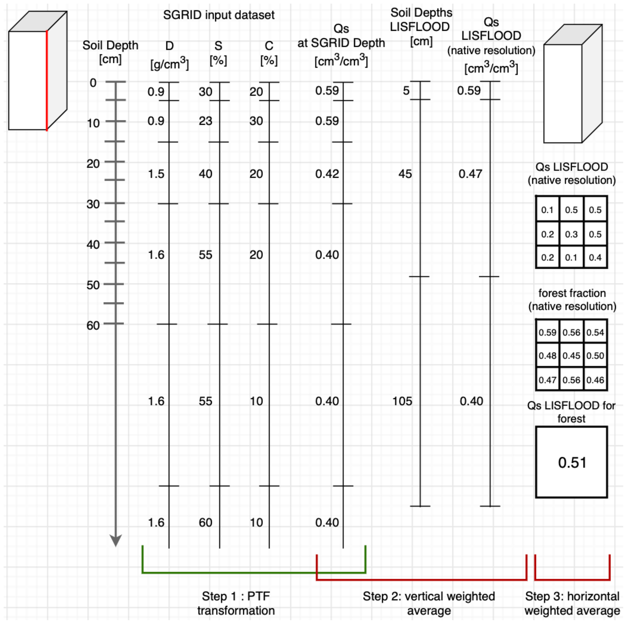
Figure C1 Creation of saturated volumetric soil moisture content parameter “Qs” using the SoilGrids250m dataset “SGRID” and forest fraction.

Appendix D

Here, more regional examples of the most interesting surface fields of CEMS_SurfaceFields_2022 are provided to show what level of detail is available at each resolution and field, as well as to emphasise consistency through all the fields, which is the most valuable requirement when running any type of surface model.

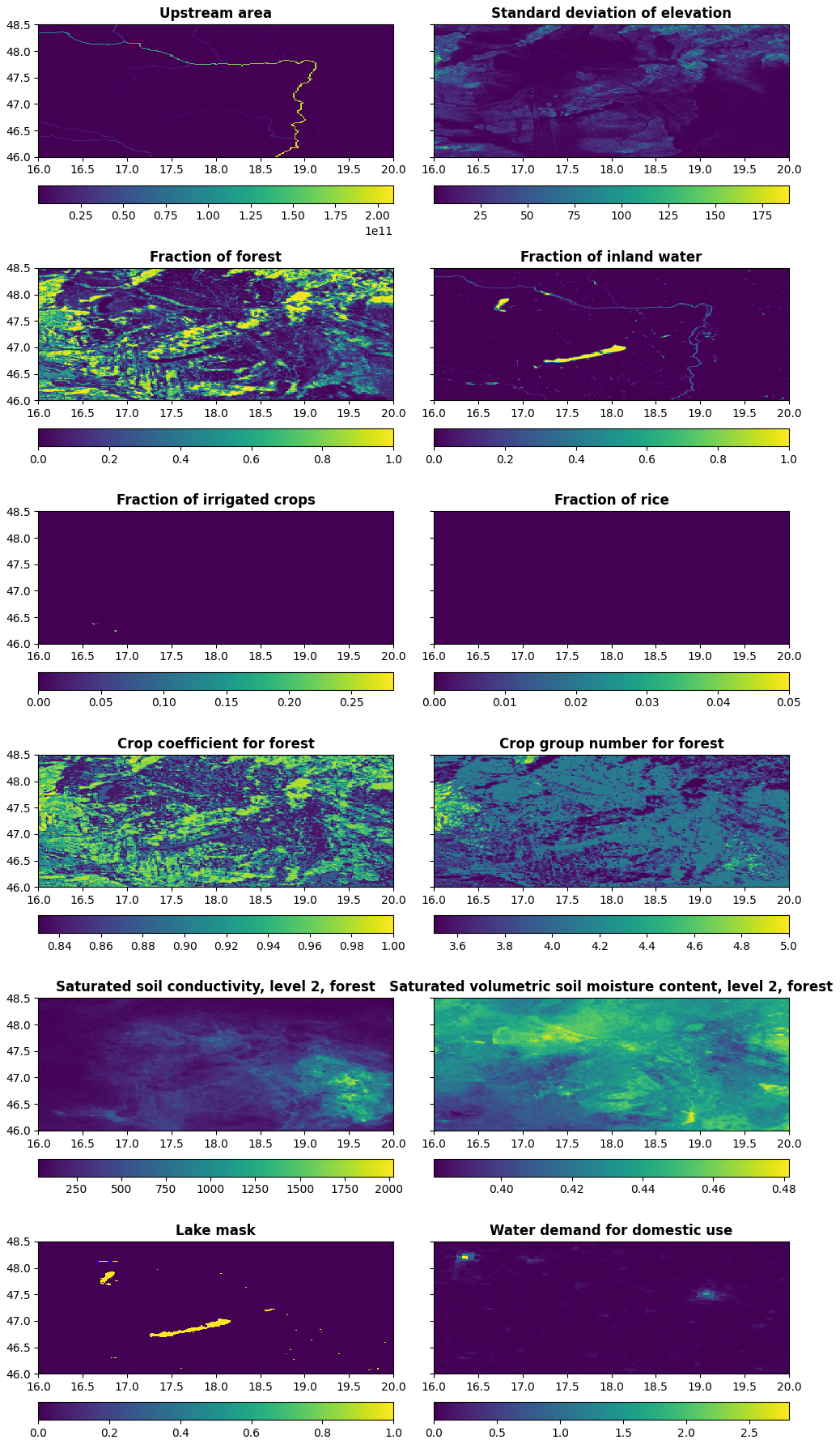
Figure D1 Upstream drainage area (in m²), standard deviation of elevation (in m), fraction of forest, fraction of inland water, fraction of irrigated crops, fraction of rice, crop coefficient for forest, crop group number for forest, saturated soil hydraulic conductivity for forested areas of soil depth layer 2 (in mm d⁻¹), saturated volumetric soil moisture (i.e. water) content for forested areas of soil depth layer 2, lake mask, and water demand for domestic use at 1 arcmin (∼ 1.9 km at the Equator) resolution for the Danube River area in Europe.

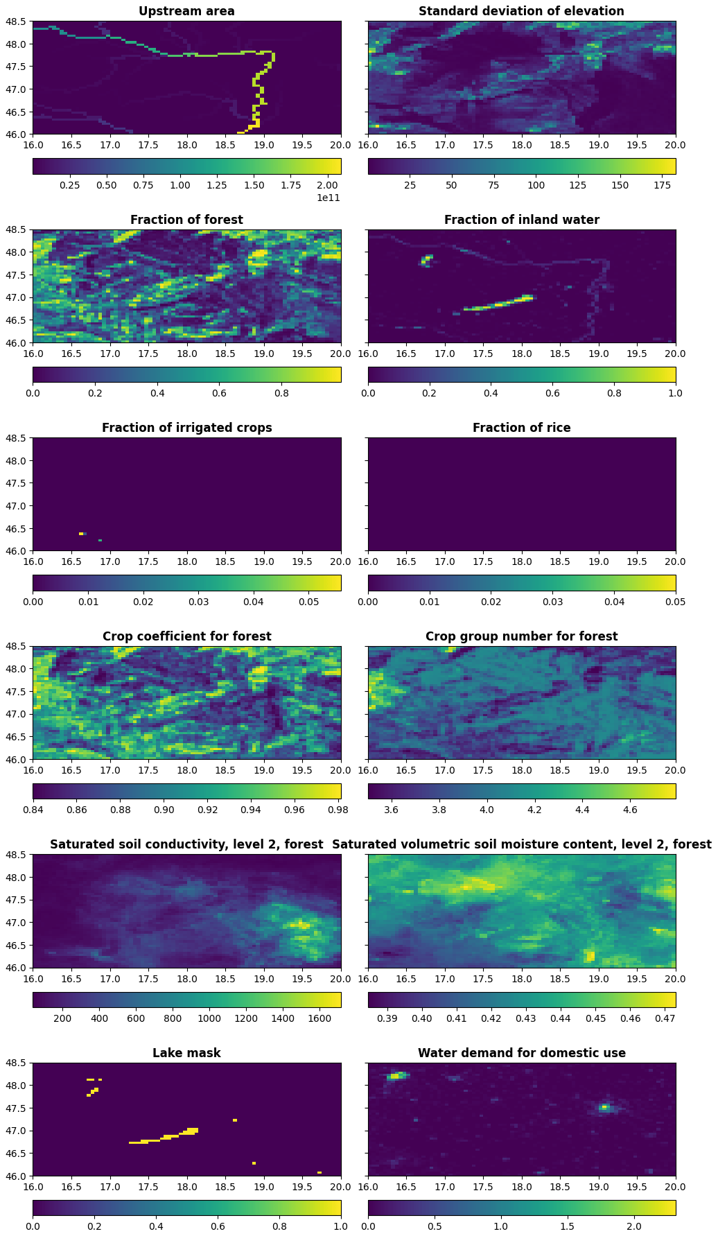
Figure D2 Same as Fig. D1 but at 3 arcmin (∼ 5.6 km at the Equator) resolution for the Danube River area in Europe.

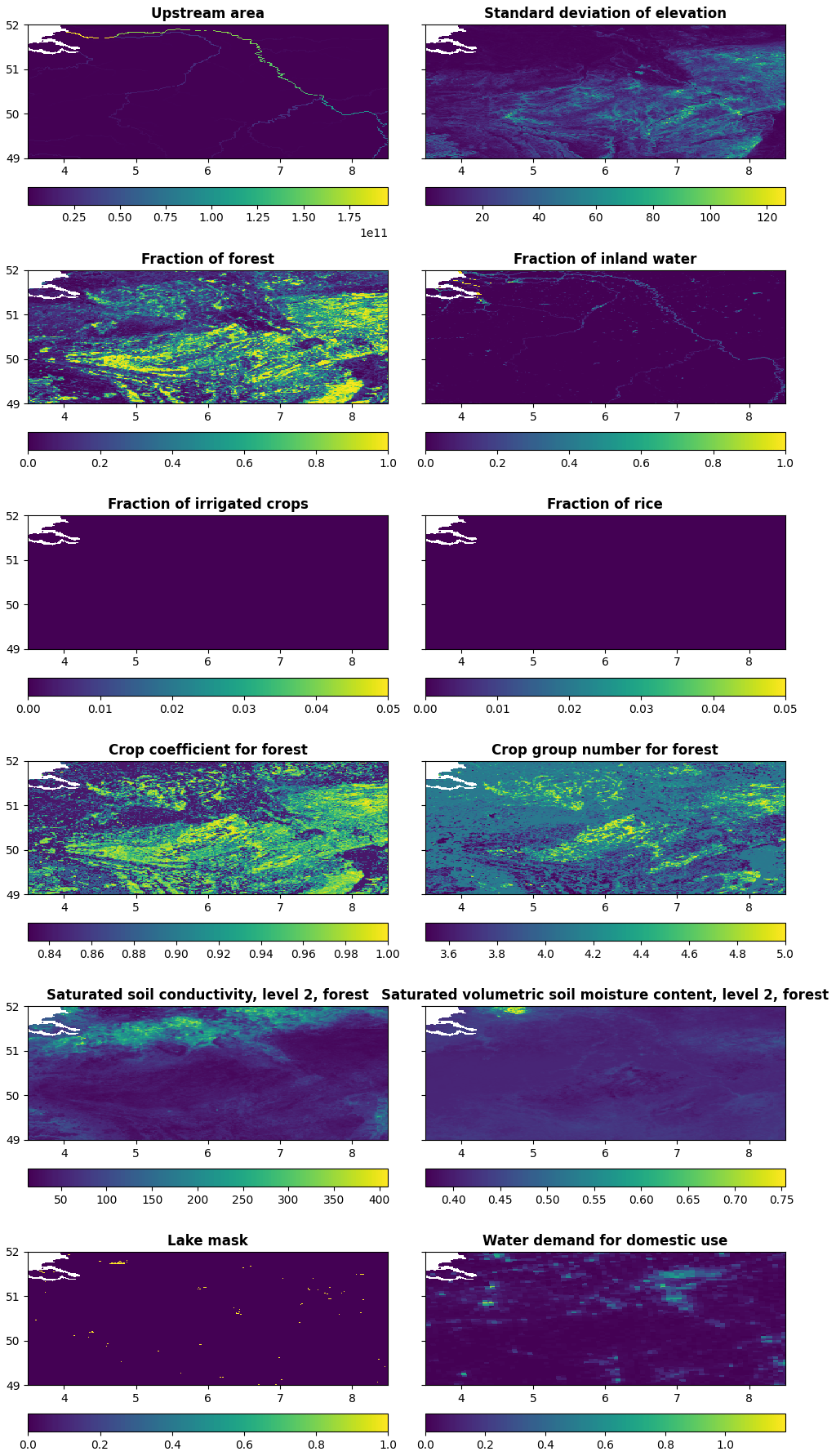
Figure D3 Same as Fig. D1 but at 1 arcmin (∼ 1.9 km at the Equator) resolution for the Rhine River area in Germany.

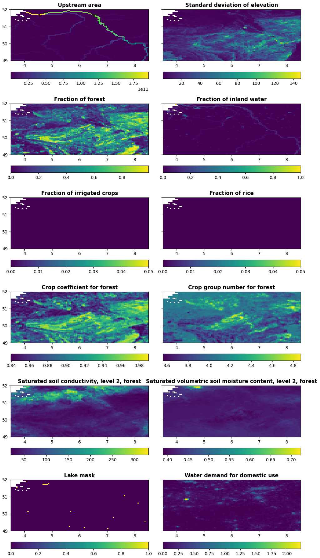
Figure D4 Same as Fig. D1 but at 3 arcmin (∼ 5.6 km at the Equator) resolution for the Rhine River area in Germany.

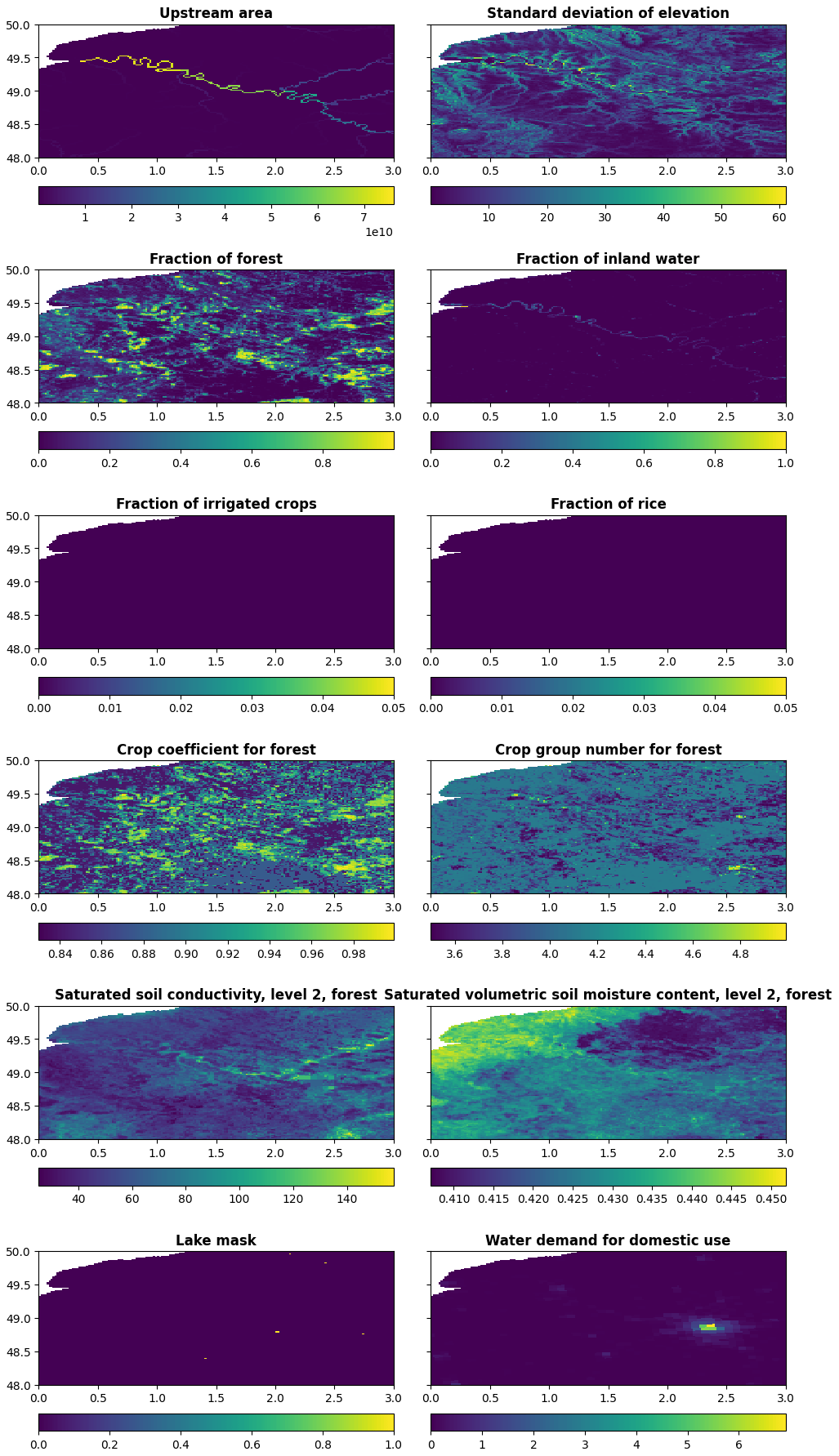
Figure D5 Same as Fig. D1 but at 1 arcmin (∼ 1.9 km at the Equator) resolution for the Seine river area in France.

Figure D6 Same as Fig. D1 but at 3 arcmin (∼ 5.6 km at the Equator) resolution for the Seine river area in France.

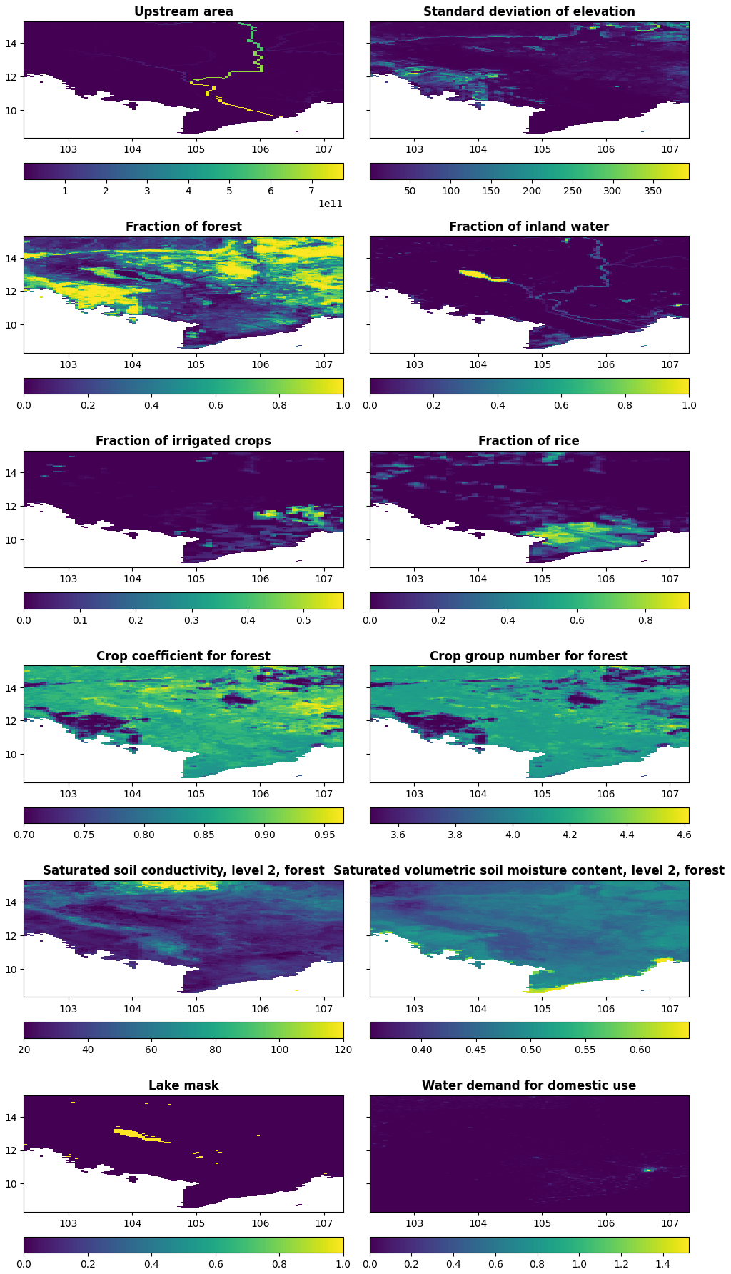
Figure D7 Same as Fig. D1 but at 3 arcmin (∼ 5.6 km at the Equator) resolution for the Mekong River area in Cambodia.