Developing a tile drainage module for the Cold Regions Hydrological Model: lessons from a farm in southern Ontario, Canada

Systematic tile drainage is used extensively in poorly drained agricultural lands to remove excess water and improve crop growth; however, tiles can also transfer nutrients from farmlands to downstream surface water bodies, leading to water quality problems. Thus, there is a need to simulate the hydrological behaviour of tile drains to understand the impacts of climate or land management change on agricultural surface and subsurface runoff. The Cold Regions Hydrological Model (CRHM) is a physically based, modular modelling system developed for cold regions. Here, a tile drainage module is developed for CRHM. A multi-variable, multi-criteria model performance evaluation strategy was deployed to examine the ability of the module to capture tile discharge under both winter and summer conditions (NSE > 0.29, RSR < 0.84 and PBias < 20 for tile flow and saturated storage simulations). Initial model simulations run at a 15 min interval did not satisfactorily represent tile discharge; however, model simulations improved when the time step was lengthened to hourly but also with the explicit representation of capillary rise for moisture interactions between the rooting zone and groundwater, demonstrating the significance of capillary rise above the saturated storage layer in the hydrology of tile drains in loam soils. Novel aspects of this module include the sub-daily time step, which is shorter than most existing models, and the use of field capacity and its corresponding pressure head to provide estimates of drainable water and the thickness of the capillary fringe, rather than using detailed soil retention curves that may not always be available. An additional novel aspect is the demonstration that flows in some tile drain systems can be better represented and simulated when related to shallow saturated storage dynamics.

1 Introduction

Harmful algal blooms and eutrophication in large freshwater lakes surrounded by agricultural lands are major environmental challenges in Canada and globally. The transport of nutrients, particularly phosphorus, in runoff from agricultural fields into surface water is an important contributor to the increased frequency of algal blooms being experienced in North America and elsewhere (Sharpley et al., 1995; Correll, 1998; Filippelli, 2002; Ruttenberg, 2005; Schindler, 2006; Quinton et al., 2010; Costa et al., 2022). Although nutrient transport from agricultural fields can occur via both surface runoff and tile drainage (Radcliffe et al., 2015), recent increases in the frequency and magnitude of algal blooms in Lake Erie in North America have been attributed to tile drainage (King et al., 2015; Jarvie et al., 2017). Tile drain systems lower seasonally high water tables in poorly drained fields and reduce the retention time of soil water, lessening waterlogging in fields and improving both crop growth and field trafficability for farmers (Cordeiro and Ranjan, 2012; Kokulan et al., 2019). However, they are also important pathways for dissolved nutrients and particulate material (Kladivko et al., 1999; Tomer et al., 2003). In Alberta, tile drains have also been used to address salinity issues (Broughton and Jutras, 2013). It has been estimated that 14 % of farmland in Canada (ICID, 2018) and 45 % of fields in southern Ontario, Canada (ICID, 2018; Vivekananthan, 2019), are drained by tile systems. Given their importance in hydrological budgets and biogeochemical transport, there is a need to understand the controlling mechanisms of water and nutrient export from tile systems as an integral part of the broader, modified hydrological system.

There are several models that can represent tile drainage, controlled tile drainage and surface runoff in different soil types at the small basin scale, which typically calculate the amount of gravitational drainage from the soil, such as HYPE (Lindstrom et al., 2010; Arheimer et al., 2015), DRAINMOD (Skaggs, 1978, 1980a; Skaggs et al., 2012), MIKE SHE (Refsgaard and Storm, 1995) and SWAT (Arnold et al., 1998; Koch et al., 2013; Du et al., 2005, 2006; Green et al., 2006; Kiesel et al., 2010). These models include conceptual components for many key hydrological processes and have been primarily designed and tested for temperate regions (Costa et al., 2020a). In Canada and other cold regions, some unique hydrological processes, such as snowmelt, rain on snow, and runoff over and infiltration into frozen or partially frozen soils, may also be important (Rahman et al., 2014; Cordeiro et al., 2017; Pomeroy et al., 1998, 2007; Fang et al., 2010, 2013). Many hydrological processes, such as the sublimation of snow, energy balance snowmelt and infiltration into frozen soils, are strongly affected by temperature and the phase changes of water, which make many existing models developed for warm regions less appropriate for regions with cold seasons (Pomeroy et al., 2007, 2013, 2016; Fang et al., 2010, 2013). Even for temperate regions, the representation of cold season processes is often underrepresented in models (Costa et al., 2020a).

Since the use of tile drainage is increasing in many cold regions (Kokulan et al., 2019; OMAFRA, 2023), it has become important to integrate such human-induced processes in the specialized hydrological modelling tools that have been developed for these regions, such as the Cold Regions Hydrological Model (CRHM) platform (Pomeroy et al., 2007, 2013, 2022). CRHM was initially developed in 1998 to assemble and explore the hydrological understanding developed from a series of research basins spanning Canada and elsewhere into a flexible, modular, object-oriented, multiphysics platform for simulating hydrological processes and basin response in cold regions (Pomeroy et al., 2007, 2022). The modular CRHM platform allows for multiple representations of forcing data interpolation and extrapolation, hydrological model spatial and physical process structure, and parameter values.

Many existing models typically operate at default daily or monthly time intervals, which is inadequate for the prediction of many short-duration “flashy” hydraulic events observed in tiles (Pluer et al., 2020; Vivekananthan, 2019; Vivekananthan et al., 2019; Lam et al., 2016a, b; Macrae et al., 2019). Indeed, the ability to simulate shorter time intervals (e.g., hourly) facilitates the ability to capture both the rising and falling limbs of tile flow hydrographs, as well as the magnitude of peak flows, both of which are important to tile drain chemistry and export (Rozemeijer et al., 2016; Williams et al., 2015, 2016; Macrae et al., 2019).

The amount of water transported by tiles depends on soil moisture dynamics, hydraulic gradients and the positioning of the saturated storage layer, which are in turn affected by many factors, including soil type, surface topography and morphology, as well as the local climate and the hydrological characteristics of the field (Frey et al. 2016; Klaiber et al., 2020; Coelho et al., 2012; King et al., 2015). Thus, to provide reliable estimations of water loss from farmland via surface runoff and tile flow, models must be able to predict soil moisture and saturated layer storage (Brockley, 1976; Rozemeijer et al., 2016; Javani-Jouni et al., 2018). Early studies have shown that in some soil types, including silty loam and clay loam soils, the drainable water is less than expected based on the effective porosity (e.g., Skaggs et al., 1978; Raats and Gardner, 1974). Raats and Gardner (1974) have argued that the calculation of drainable porosity requires knowledge of water table elevation and the distribution of soil moisture above the saturated storage layer. Skaggs et al. (1978) added that the calculation of drainable porosity should consider “the unsaturated zone drained to equilibrium with the water table”. However, because the soil column is often composed of different soil layers with varying physical characteristics, drainable porosity varies with evapotranspiration rate, soil water dynamics and the depth of saturated water (Logsdon et al., 2010; Moriasi et al., 2013). In a sandy loam soil, Lam et al. (2016a, b) demonstrated that tile drainage was not initiated until soil was at or above field capacity. Williams et al. (2019) observed in the American Midwest that tile drainage was not initiated until the field storage capacity had been exceeded. It has also been shown that, despite the presence of tile drains, the soil above the tile did not always drain all the gravitational water following a rainfall/snowmelt event, and the soil may remain at or above field capacity (Skaggs et al., 1978; Lam et al., 2016a). This means that the soil drainable water content may be considerably smaller than the storage capacity. This is related to matric potential within the vadose zone, which is driven by the soil characteristics but can also be due to the development of a capillary fringe that reduces the rate of vertical percolation through the unsaturated zone, reducing tile flow (Youngs, 2012). Despite this evidence, some saturated flow models that simulate tile flow overlook the effect of capillary rise and overestimate the soil drainable water. Other models that represent unsaturated flow (i.e., HYDRUS 3D; Simunek et al., 2024) using Richard's equation (Richards, 1931) capture the effect of capillary rise and saturation-pressure variation within the soil profile and assess the soil drainable water more accurately. Although the effect of capillary rise is considered in DRAINMOD through the concept of drainable porosity (represented as a “water yield”) (Skaggs, 1980b) and is calculated for layered soil profiles (Badr and Skaggs, 1978), it requires detailed information surrounding the soil water characteristic curve (Skaggs, 1980b). Although it is indeed optimal to use soil-specific water characteristic curves, Twarakavi et al. (2009) found that it is possible to employ average representative values from the soil water characteristic curve to represent soil drainable water where soil-specific curves are not available, with some reduction in model performance.

In this study, a new tile drainage module (TDM) was developed and incorporated within the physically based, modular Cold Regions Hydrological Model (CRHM) platform (Pomeroy et al., 2022) to enable hydrological simulations in tile-drained farm fields in cold agricultural regions. As a first iteration, the new module was developed for a field with sloping ground and loam soil with imperfect drainage. Such landscapes are common in the Great Lakes region (e.g., Michigan and Vermont, USA, and Ontario, Canada), and tile drainage in such landscapes has not been as widely studied as it has been in clay-dominated soil. In this module, considerations were explicitly included for the effects of capillary rise and annual fluctuations in saturated storage on drainable soil water storage. The use of field capacity and groundwater/soil-saturated storage (Twarakavi et al., 2009) to modulate soil drainable water across the soil profile, including the capillary fringe region, is an innovative aspect of the model that has been demonstrated to circumvent the need for water characteristic curves. The development of this physically based module provides insight into hydrological processes in tile drainage from sloping landscapes with imperfect drainage, which are increasingly being artificially drained (Cordeiro and Ranjan, 2012; Kokulan et al., 2019; OMAFRA, 2023).

2 Materials and methods

2.1 Study area

The study site is an ∼10 ha farm field located near Londesborough, Ontario, at UTM 17T 466689 m E 4832203 m N, shown as LON in Fig. 1a. Mean annual precipitation recorded in this region is 1247 mm (ECCC, 2020). Mean air temperature is 7.2 °C, with annual maxima in July (25.9 °C) and minima in January (−10.2 °C) (ECCC, 2020). Soil type has been identified as Perth clay loam (Gray Brown Luvisolic), with a slope between 0.2 % and 3.5 %. The field is systematically drained with a tile depth of 0.9 m and a spacing of 14 m (laterals). The tile network collects infiltrated water from about 75 % of the field (∼7.6 ha) but may also receive lateral groundwater flow from neighbouring fields. Water yields from the tile drain laterals (10 cm diameter) are discharged via a common tile outlet (main, 15 cm diameter) below ground. Surface runoff from the field is directed toward a common outlet on the surface using plywood berms installed along the field edge (see Van Esbroeck et al., 2016). The tile and surface runoff outlets do not join into a common outlet and are fully separated from one another, even during surface ponding events. The field uses a corn–soy–winter-wheat rotation system with cover drops and rotational conservation till (shallow vertical tillage every 3 years). Additional details related to farming practices are provided in Plach et al. (2019), soil characteristics are provided in Plach et al. (2018a) and Plach et al. (2018b), and equipment and monitoring are provided in Van Esbroeck et al. (2016). The outlets for both surface and tile flow are located at the edge of the field and drain into an adjacent field (Fig. 1b). Water tends to accumulate in a topographic low in the field, in front of the field outlet during snowmelt or high-intensity rainfall events, presumably due to either surface runoff or return flow (see ponded area, Fig. 1b). However, surface water or elevated soil moisture conditions are not observed in this topographic low during smaller events or dry periods of the year, suggesting that this saturated ponding is not in a perennial groundwater discharge zone. Although surface ponding is observed in the topographic depression within the field, water discharges freely at the opposite end of the culvert, facilitating the measurement of flow.

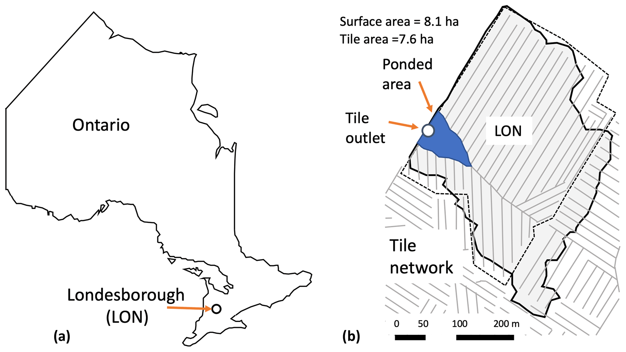
Figure 1 (a) Location of the study area in the south of Ontario and the (b) Londesborough (LON) farm with its tile network.

2.2 CRHM: the modelling platform

CRHM is a modular hydrological process modelling platform that allows users to select relevant process modules and apply them as needed to their study. For example, the CRHM platform includes options for empirical and physically based calculations of precipitation phase, snow redistribution by wind, snow interception, sublimation, sub-canopy radiation, snowmelt, infiltration into frozen and unfrozen soils, hillslope water movement, actual evapotranspiration, wetland fill and spill, soil water movement, and groundwater flow and streamflow (Pomeroy et al., 2007, 2022). Where appropriate, it is able to calculate runoff from rainfall and snowmelt as generated by infiltration excess and/or saturated overland flow, flow over partially frozen soils, detention flow, shallow subsurface flow, preferential flow through macropores and groundwater flow (Pomeroy et al., 2007, 2022). Modules of a CRHM model can be customized to basin setup, such as delineating and discretizing the basin, conditioning observations for extrapolation, and interpolation in the basin, or are process-support algorithms such as for estimating longwave radiation, complex terrain wind flow, or albedo dynamics, but most modules address hydrological processes such as evapotranspiration, infiltration, snowmelt and streamflow discharge. CRHM discretizes basins into hydrological response units (HRUs) for mass and energy balance calculations, each with unique process representations, parameters and positions along flow pathways in the basin. HRUs are connected by blowing snow, surface, subsurface and groundwater flow and together generate streamflow which is routed to the basin outlet. The size of the HRUs is flexible and can be as small as the size of a single tile pipe (e.g., 1 m) times the pipe spacing (which was 14 m in our case study region) and as large as entire tile networks within a given farm or study area. CRHM does not require a stream within a modelled basin. The feature allows CRHM to model the hydrology of cold regions dominated by storage and episodic runoff, such as agricultural fields.

Although CRHM has the capability to represent many hydrological and thermodynamic processes, not all processes need/must be represented in all situations. The modular design of the CRHM platform enables the user to activate or inactivate specific processes to optimize the model for a particular situation. This is a modelling approach that enables testing different modelling hypotheses and has been pioneered by CRHM and other models, which has inspired a range of hydrological (e.g., SUMMA; Clark et al., 2015a, b), hydrodynamic (e.g., mizuRoute; Mizukami et al., 2016) and biogeochemical (e.g., OpenWQ; Costa et al., 2023) modelling tools. For example, in the current study, blowing snow was not employed in CRHM as it does not appear to be significant at the study site (periodic snow surveys showed relatively uniform snow cover). Similarly, preferential flow into tile drains was not included in the current simulation. Although it can be a key process in some clay loam soils, previous studies at the study site have shown that it is not the case here, which is a combination of clay-loam and silt-loam soils (Pluer et al., 2020; Macrae et al., 2019). Hydrograph analysis (Macrae et al., 2019) and conservative tracer analysis (electrical conductivity and major ions, as well as temperature) over multiple years (Pluer et al., 2020) showed that preferential flow was minimal at this site as well as other similar sites. Freeze–thaw of soil can occur in the study region, leading to partially frozen soils. However, the extent of freezing varies with snowpack development, winter temperatures and radiation. Data collected over an 8-year period at this site found soil freezing was restricted to brief periods and such freezing never extended below 10 cm depth (Macrae, unpublished data), which is insufficient for soils to behave as frozen ground for infiltration calculations. Consequently, freeze–thaw processes were not deployed in the CRHM model of this site.

2.3 Observations and input data for the model

Tile flow, water table elevation (saturated storage elevation head) and surface flow were measured at the site between October 2011 and September 2018 at 15 min intervals. It was not possible to install more than one measuring station for water table elevation and soil moisture at the site due to farming activity; consequently, water table elevation head and soil moisture were measured at the approximate midpoint of the field at the edge of the field. Both tile flow rates and surface runoff were determined using simultaneous measurements of flow velocity and water depths in each of the pipes at the edge of the field using Hach FLO-TOTE sensors and an FL900 data logger (Onset Ltd.) (Table A1, Appendix A). Continuous measurements of velocity were included due to the potential for impeded drainage under very wet conditions or caused by the accumulation of snow and ice around the surface culvert in winter. An additional barometrically corrected pressure transducer (U20, Onset Ltd.) (Table A1) was also used for periods when the flow sensors did not function, using a rating curve developed from the depth–velocity sensors; however, it should be noted that these were for brief periods and the depth–velocity sensor functioned for the majority of the study. The water table elevation was measured using a barometric pressure-corrected pressure transducer (U20, Onset Ltd.).

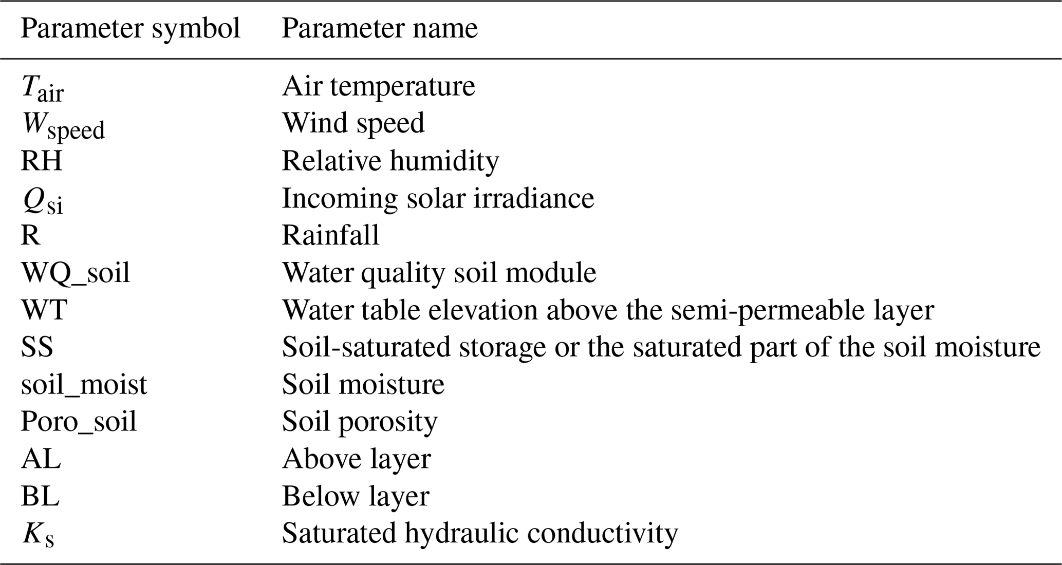
Air temperature, wind speed, air relative humidity, incoming solar irradiance and rainfall were also measured at the site at 15 min intervals and were implemented in the model. Variable names and their symbols in CRHM are listed in Appendix B. The air temperature, wind speed and incoming solar radiance measurements were collected 1 m above ground using a temperature smart sensor S-THB-M002, wind smart sensor set S-WSET-M002 and a solar radiation sensor (Table A1). Rainfall and relative humidity were measured via a tipping bucket rain gauge (Table A1) and an RH smart sensor (Table A1). These observations were continuously recorded throughout the study period, except for brief periods of instrument failure and maintenance, when data from nearby stations were substituted using the double mass analysis method (Searcy and Hardison, 1960).

Although rainfall was recorded continuously at the field site, snowfall data were not. Snowfall data were obtained from nearby stations (Wroxeter-Davis and Wroxeter; ECCC, 2020), located 31.7 km from the field site. Periodic snow surveys done at the site throughout the study period found that data from the nearby stations were a close approximation of snow at the field site (Plach et al., 2019). Hourly snowfall observations from Wroxeter-Geonor were used for the period between 2015 and 2018, whereas daily data from the Wroxeter-Geonor were used for the 2011 to 2014 period, reconstructed to hourly snowfall time series based on the method presented by Waichler and Wigmosta (2003).

2.4 Development of the new tile module

A tile drainage module (TDM) was developed within CRHM (Figs. 2, 3) with the goal of adding the ability to simulate tile flow and the resulting saturated storage at an hourly time step. CRHM was forced with hourly precipitation, air temperature, solar radiation, wind speed and relative humidity to calculate hydrological states and fluxes in HRUs and the basin. The model requires parameterizations that specify the hydraulic and hydrological properties of the soil, including its thickness, saturated hydraulic conductivity (K) and surface cover. CRHM calculates water storage and fluxes between HRUs, as well as vertical fluxes amongst different hydrological compartments (within each HRU) that include snow, depressional storage, different soil layers and groundwater.

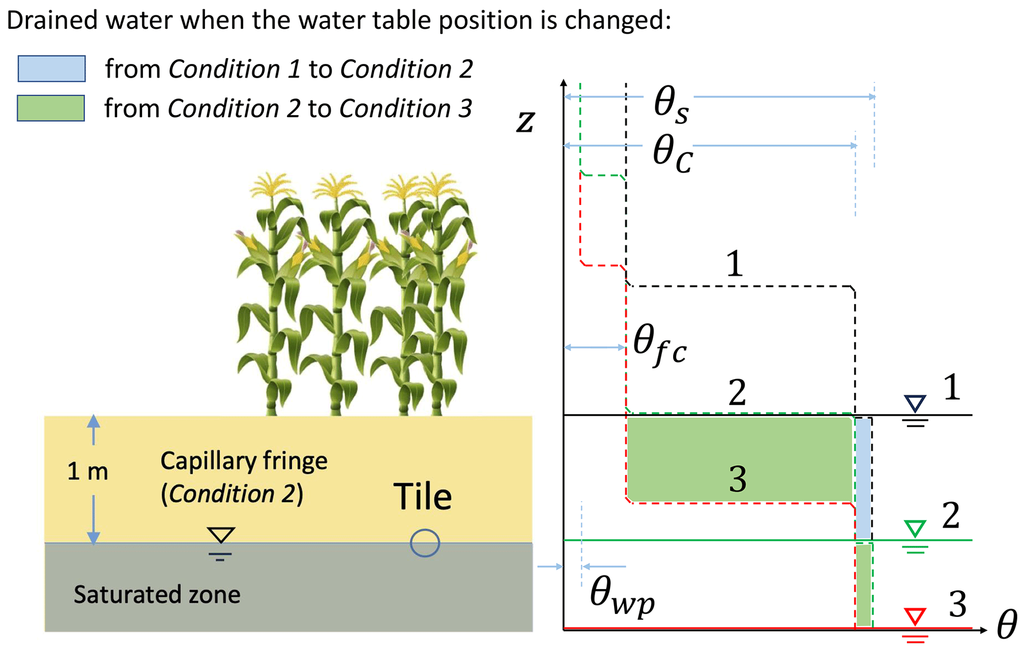
Figure 2 Schematic representation of the capillary fringe above the water table assuming a 1 m thickness (for demonstration purposes). The soil characteristic curves are shown for the three water level conditions considered: water level at the (1) surface, (2) intermediate depth and (3) deeper depth. Two transitional drops can be seen in the characteristic curves: one from saturation (θ_s) to capillary fringe water content (θ_C) (between conditions 1 and 2) and one from θ_C to field capacity (θ_fc) (between conditions 2 and 3). The coloured areas (green and blue) of the right panel correspond to the amount of water that can be released between conditions 1 and 2 (blue) and between conditions 2 and 3 (green).

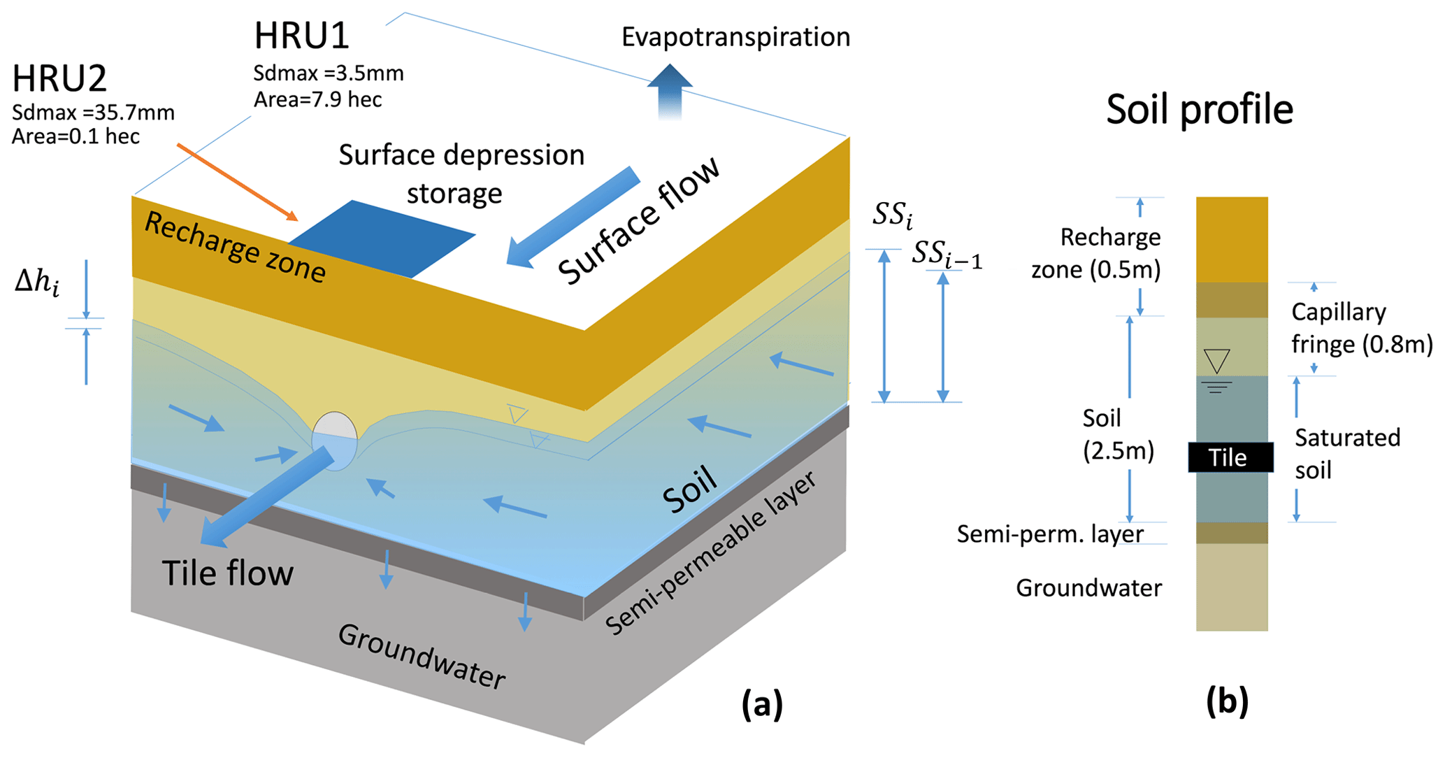
Figure 3 (a) Schematic conceptual view of the CRHM model configuration, including soil layers, saturated storage (SS), groundwater and tile flow; (b) soil profile, including the capillary fringe and its location relative to the soil and tile.

Using the simulation of soil moisture (including both saturated and unsaturated soil moisture) performed by the original CRHM “Soil” module, the TDM calculates the dynamic tile flow rate that, in turn, feeds back to soil moisture at each time step. The presence of a capillary fringe (sometimes referred to as the tension-saturated zone within the soil profile) and its effects are considered by limiting the amount of drainable soil water. The TDM uses site-specific information regarding the tile network, such as tile depth, diameter and spacing. Information regarding site-specific details regarding tile depth, diameter and spacing may be obtained directly from landowners or can be estimated based on standard design and installation guidelines for the region. This information was used to set up the model together with parameterization to translate the hydrological effects of the soil capillary fringe (CF), if present, through two variables: CF thickness and CF drainable water (discussed in Sect. 2.5, Figs. 2, 3). These two variables are used to limit the fraction of the soil moisture that can freely drain to the tiles.

2.4.1 Soil moisture and saturated storage

The TDM uses the water quality soil module or the soil module (WQ_soil or Soil), which divides the soil column into three layers: a recharge layer where evapotranspiration and root uptake generally take place, a deeper layer that connects to the groundwater system and a deeper groundwater layer that is always saturated. CRHM's state variable for soil moisture in the upper two layers is soil water storage volume (Fig. 2); the model results were converted into water table elevation above the semi-permeable layer (Table B1, Appendix B; Fig. 2b) for comparison with water table observations, by dividing volumetric soil moisture content (Table B1) by soil porosity (Table B1) for the cases with no capillary fringe above the water table. Additional steps were taken for periods when a capillary fringe developed (discussed below).

2.4.2 Capillary fringe and drainable water

Soil moisture in the capillary fringe is equal to the average volumetric water content at capillary fringe (θ_C), which is usually greater than the field capacity (θ_fc) (Bleam, 2017, Sect. 2.4). Therefore, while the positioning of the capillary fringe responds dynamically to the matric potential, the saturation profile within the capillary fringe remains constant, as well as its thickness, because it only depends on the pressure head (capillary forces) that is related to the grain size distribution and field capacity (h_fc) as introduced by Twarakavi et al. (2009). Therefore, the drainable water in the capillary fringe becomes the difference between saturation (θ_s), computed dynamically in CRHM, and θ_C, which corresponds to the water held by capillary forces at the capillary fringe moisture content (Fig. 2). Accordingly, Fig. 2 shows the schematic soil characteristic curve for the three water level conditions contemplated in the model.

1. Condition 1 is when the water table is at the surface and the soil is completely saturated (matric potential = 0).

2. Condition 2 is when the water table drops but the upper boundary of the capillary fringe is at the soil surface.

3. Condition 3 is when the water table drops further, and the upper boundary of the capillary fringe drops beneath the surface.

In essence, the soil is completely saturated (θ_s) in condition 1. Between conditions 1 and 2, the capillary fringe occupies the entire soil column above the water level; thus, it can only release the volume of water corresponding to θ_s−θ_C or φ_c (dimensionless). Between conditions 2 and 3, two layers with distinct hydraulic characteristics develop: (1) the top one at θ_fc that releases water up to θ_C−θ_fc and (2) the lower one that corresponds to the capillary fringe and can release up to the volume of water corresponding to θ_s−θ_C or φ_c.

2.4.3 Tile flow calculation

A modified version of the Hooghoudt equation was used to calculate tile flow in the TDM (Smedema et al., 2004). This presumes no surface ponding, an assumption that generally holds at the study site (Eq. 1), where water ponds only during very wet periods and on a small portion of the study site (see Fig. 1b). Hooghoudt's equation (Hooghoudt, 1940) is a steady-state, physically based equation for saturated flow toward the tile drain. Flow estimates are provided based on the hydraulic conductivity of the soil and water table elevation above the tile pipe. It allows for different saturated hydraulic conductivities for the layers above (AL) and below (BL) the tile (Fig. S1). At the study site, soil surveys have reported almost the same soil type (loam) down to a depth of 90 cm (e.g., Van Esbroeck et al., 2016; Plach et al., 2018b), which was parameterized in the model set up as

$$\begin{array}{}\text{(1)}& q={\displaystyle \frac{\mathrm{8}\times K_{\mathrm{2}}\times d\times h}{L^{\mathrm{2}}}}+{\displaystyle \frac{\mathrm{4}\times K_{\mathrm{1}}\times h^{\mathrm{2}}}{L^{\mathrm{2}}}},\end{array}$$

where K₁ and K₂ are respectively the saturated hydraulic conductivity in the upper and lower layers (in mm h⁻¹), L is the tile spacing (in mm), h is the water table elevation above the tile (in mm), d is the lower layer thickness (in mm) (Fig. S1), and q is the predicted tile flow (in mm h⁻¹). The only variable that is dynamically updated by CRHM is h. Equation (1) was used to estimate tile flow rates in the TDM, using saturated storage to estimate h.

2.4.4 Calculation of the effect of tile flow on soil moisture and water levels

The simulated tile flows (see Sect. 2.3.3) were subtracted from the soil moisture. To calculate saturated storage (water table or groundwater elevation head level) from soil moisture calculated by the model, a threshold soil moisture content (sm_t) is defined, which consists of drainable water in the soil (φ_c) when the upper boundary of the capillary fringe is at the surface (condition 2, Fig. 2) and was calculated as

$$\begin{array}{}\text{(2)}& {\mathrm{sm}}_{\mathrm{t}}={\mathrm{sm}}_{\max }-\left(C_{\mathrm{t}}\times {\mathit{\phi }}_{\mathrm{c}}\right),\end{array}$$

where sm_max is the maximum soil moisture  and C_t is the capillary fringe thickness (in mm). However, since the hydrological conditions of the soil are markedly different between the two transitional situations described in Sect. 2.3.2 and Fig. 2 (condition 1 to 2 and condition 2 to 3), a step function was deployed for determination of saturated storage:

$$\begin{array}{}\text{(3)}& \mathrm{SS}=\left\{\begin{array}{l}\frac{{\mathrm{sm}}_{\mathrm{t}}-\left(C_{\mathrm{t}}\times \left(\left({\mathit{\phi }}_{\mathrm{s}}-{\mathit{\phi }}_{\mathrm{c}}\right)+{\mathit{\theta }}_{\mathrm{fc}}\right)\right)}{{\mathit{\phi }}_{\mathrm{s}}+{\mathit{\theta }}_{\mathrm{fc}}}+\frac{\mathrm{sm}-{\mathrm{sm}}_{\mathrm{t}}}{{\mathit{\phi }}_{\mathrm{c}}}\\ \mathrm{if}\mathrm{between}\mathrm{conditions}\mathrm{1}\mathrm{and}\mathrm{2},\\ \frac{{\mathrm{sm}}_{\max }}{{\mathit{\phi }}_{\mathrm{s}}+{\mathit{\theta }}_{\mathrm{fc}}}-\left(\left(\frac{{\mathrm{sm}}_{\mathrm{t}}-\mathrm{sm}}{{\mathit{\phi }}_{\mathrm{s}}}\right)+C_{\mathrm{t}}\right)\\ \mathrm{if}\mathrm{between}\mathrm{conditions}\mathrm{2}\mathrm{and}\mathrm{3},\end{array}\right.\end{array}$$

where SS is saturated storage (in mm) from the bottom of the soil, and sm is soil moisture (both saturated and unsaturated storage) in the given time step (in mm). Water table observations were used to estimate SS from the field. Equation (3) is determined based on soil moisture curves in Fig. 2 and water level conditions 1–3 discussed in Sect. 2.3.2. In Fig. 2, the first and second parts of Eq. (3), which refer to conditions 1 to 2 and 2 to 3, respectively, correspond to the volumes of soil water highlighted in blue and green.

2.4.5 Lower semi-permeable soil layer and periodicity in annual groundwater levels

This model application focused on the study site field without including other adjacent areas. This was possible because years of field monitoring at this site have demonstrated that there is no observable surface flow into the site from adjacent fields. The tile network is restricted to the field and is not connected to tile drains or surface inlets in adjacent fields. However, field soil water table observations show evidence of annual groundwater level periodicity/fluctuation (Rust et al., 2019) that is sinusoidal in nature and cannot be neglected. Some studies predict the annual groundwater oscillations or the annual responses of groundwater to precipitation by using sine and cosine functions (De Ridder et al., 1974; Malzone et al., 2016; Qi et al., 2018). De Ridder et al. (1974) studied the design of the drainage systems and described the seasonal groundwater fluctuations observed in wells using sinusoidal curves. Malzone et al. (2016) used a sine function to predict annual groundwater fluctuations in the hyporheic zone. Qi et al. (2018) and Rust et al. (2019) used a cross-wavelet transform, consisting of the superposition of sine and cosine curves, to predict shallow groundwater response to precipitation at the basin scale. This approach, using the sine function, was used in this application to simulate annual fluctuations in saturated storage, in Eq. (4), over a period of 1 year, with minimums around the middle of the growing season (mid-July) and maximums in the cold season (early February). This translates into the greater matric potential, with soil moisture depletion, during the growing season and lower matric potential, with soil moisture increases, during the non-growing season, consistent with field observations. Thus, a sine function representing the annual fluctuations in percolation rate from soil to groundwater (G_y,i) layers in CRHM, through the lower soil semi-permeable layer (in mm h⁻¹), is defined as

$$\begin{array}{}\text{(4)}& G_{y,i}=\left[A\times \sin \left({\displaystyle \frac{\left(T_{\mathrm{s}}-D_{\mathrm{d}}\times \mathrm{24}\right)\times \mathrm{360}}{\mathrm{24}\times \mathrm{365.25}}}\right)-B\right]\times f_{y,i},\end{array}$$

where T_s is the time step number, D_d is a time delay in days, A is the amplitude of the saturated storage (SS) fluctuation and B is an intercept factor. f_y,i is a seasonal factor. The sine function coefficients (D_d, A and B) and seasonal factor were adjusted for the whole period and for each year through model verification and are shown in Table 1. Appendix C provides more details on the implementation of Eq. (4). Although this is a simplification of the entire groundwater system dynamics, it was needed here to provide a more controlled basis for testing the new module at the field scale before expanding it to larger areas in future work.

2.5 Model application and multi-variable, multi-metric validation

The study site is a relatively small field, and 2 HRUs were sufficient to capture its hydrological dynamics in CRHM. The HRUs represent (1) the area immediately upstream of the outlet where surface ponding occurs (depression storage) and (2) the remaining field (Fig. 3). The maximum ponding capacity of HRU1 was estimated using the spatially distributed hydrodynamic model FLUXOS-OVERFLOW (Costa et al., 2016, 2020b). The CRHM model with its new TDM module was set up using the information described in Table 1. Soil textures at the LON site measured in a 25 m grid across three soil depths (0–25 cm, 25–50 cm and 50–100 cm) averaged 29 % sand, 48 % silt and 23 % clay (Ontario Ministry of Agriculture, Food and Rural Affairs Soil Team, unpublished data). This soil grain size distribution corresponds with a soil-saturated hydraulic conductivity of ∼0.56 cm h⁻¹ ($\sim {\mathrm{10}}^{-\mathrm{2.5}}$) (García-Gutiérrez et al., 2018), which was implemented in CRHM (0.5 cm h⁻¹), corresponding to a field capacity of 0.04 (volumetric water content) and h_fc of ∼0.8 m (Twarakavi et al., 2009, based on a drainage flux of 0.1 cm d⁻¹).

A robust multi-variable, multi-metric model evaluation strategy was deployed to verify the capacity of the model to predict tile flow and its impact on the local hydrology. The outflows examined were tile flow, surface flow and saturated storage. The multi-metric approach contemplated five different methods, namely the Nash–Sutcliffe efficiency (NSE), root-mean-square error (RMSE), model bias (Bias), percentage bias (PBias) and RMSE-observation standard deviation ratio (RSR). These methods were used to assess model accuracy. See Appendix C for more details about the methodology used. It is generally assumed that NSE>0.50, RSR≤0.70 and PBias in the range of ±25 % are satisfactory for hydrological applications (Moriasi et al., 2007). Five different metrics were used to evaluate model accuracy in order to describe different aspects of the discrepancies between simulated and observed values. For example, the model bias reveals the positive or negative general deviations of simulated values from the observed values, while RMSE shows the average absolute differences between them (Moriasi et al., 2007). Hourly values were used in these calculations, which departs from the daily and monthly analyses typically reported for these types of models. Although the hourly time step is challenging for this sort of simulation, it is an important advance forward toward more detailed, accurate and advanced models for tile-drained agricultural fields. For example, Costa et al. (2021) noted that the successful extension of hydrological models to water quality studies relies on their ability to operate at short timescales in order to capture intense, short-duration storms that may have a disproportional impact on the runoff transport of some chemical species such as phosphorus – in essence, to capture hot spots and hot moments for flux generation.

Table 1 Key model parameters in CRHM for representation of the LON site.

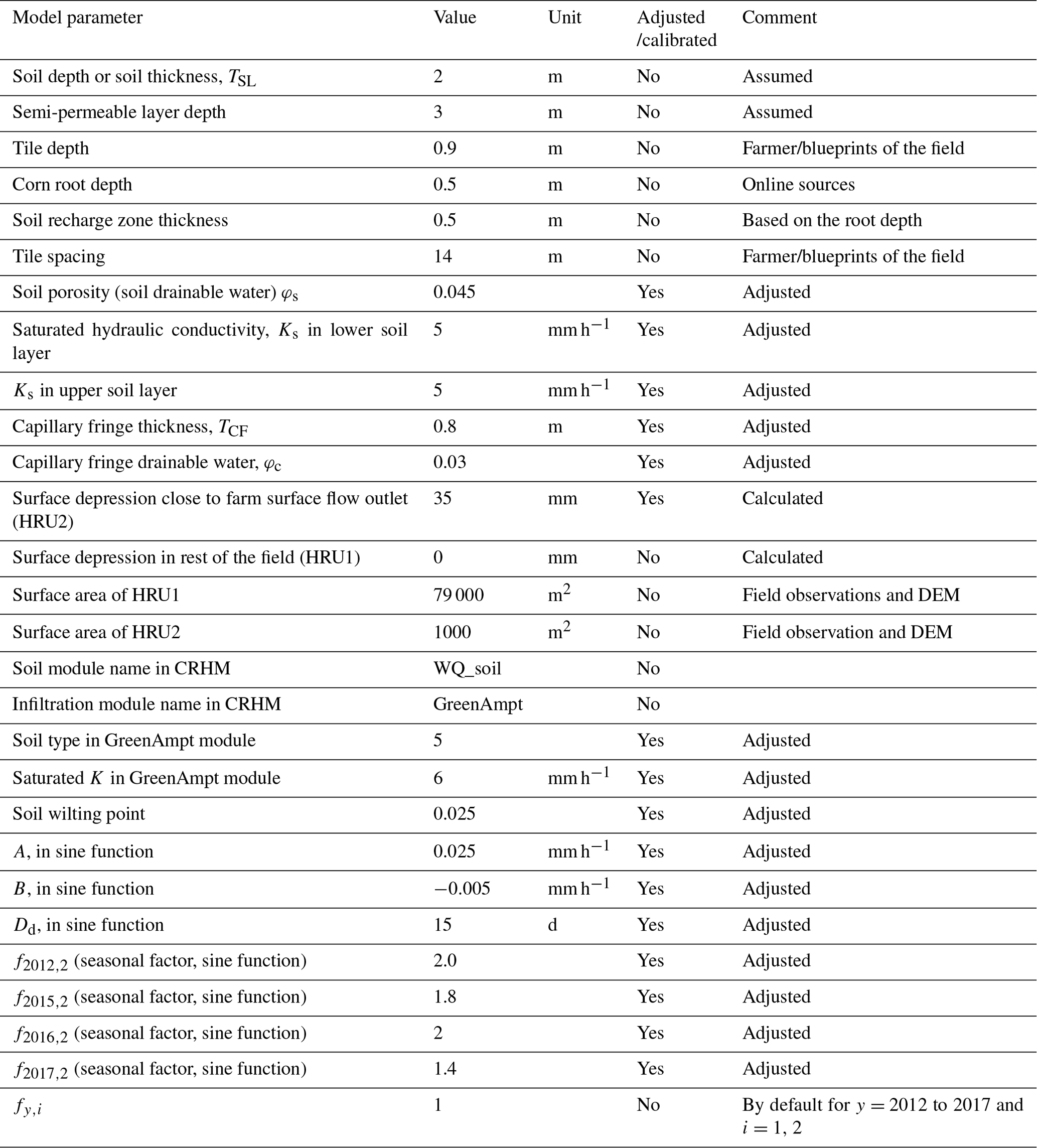
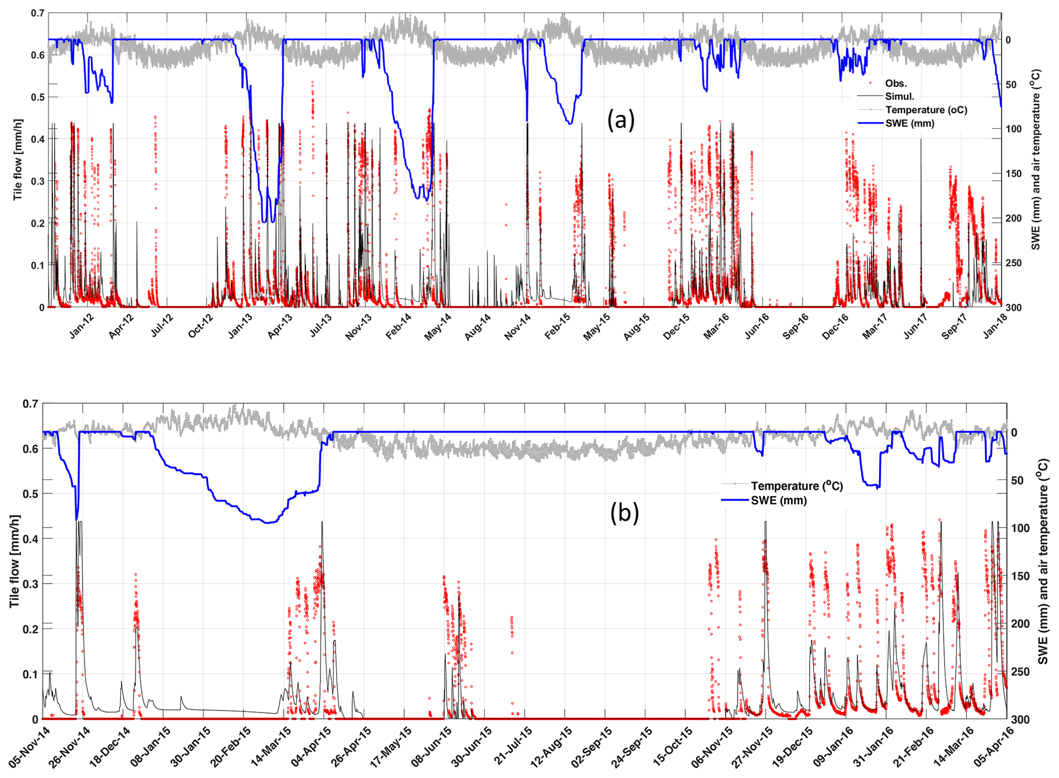
Figure 4 Comparison between observed and simulated tile flows, simulated SWE (snow water equivalent) and observed air temperature in the LON site, between October 2011 to January 2018 (a) and between November 2014 to April 2016 (b).

3 Results

A multi-variable, multi-metric model evaluation approach was deployed to verify the capacity of the model to predict not only tile flow but also the effects it has on the local hydrology, from surface to subsurface processes. The outflows examined were tile flow (Sect. 3.1), saturated storage (Sect. 3.2) and surface flow (Sect. 3.3). The multi-metric approach contemplated five different methods, namely the Nash–Sutcliffe efficiency (NSE), root-mean-square error (RMSE), model bias (Bias), percentage bias (PBias) and RMSE-observation standard deviation ratio (RSR).

3.1 Tile flow

The model was able to capture most tile flow events, both in terms of the timing and magnitude of peak flows and the most important seasonal patterns (Fig. 4). For example, the near absence of flow during the growing season (May to September) was captured. The simulated flow peaks generally had a good agreement with observations, as well as the low flow or base flows during cold periods (December–March). The ascending and descending limbs of the response signal were also adequately predicted.

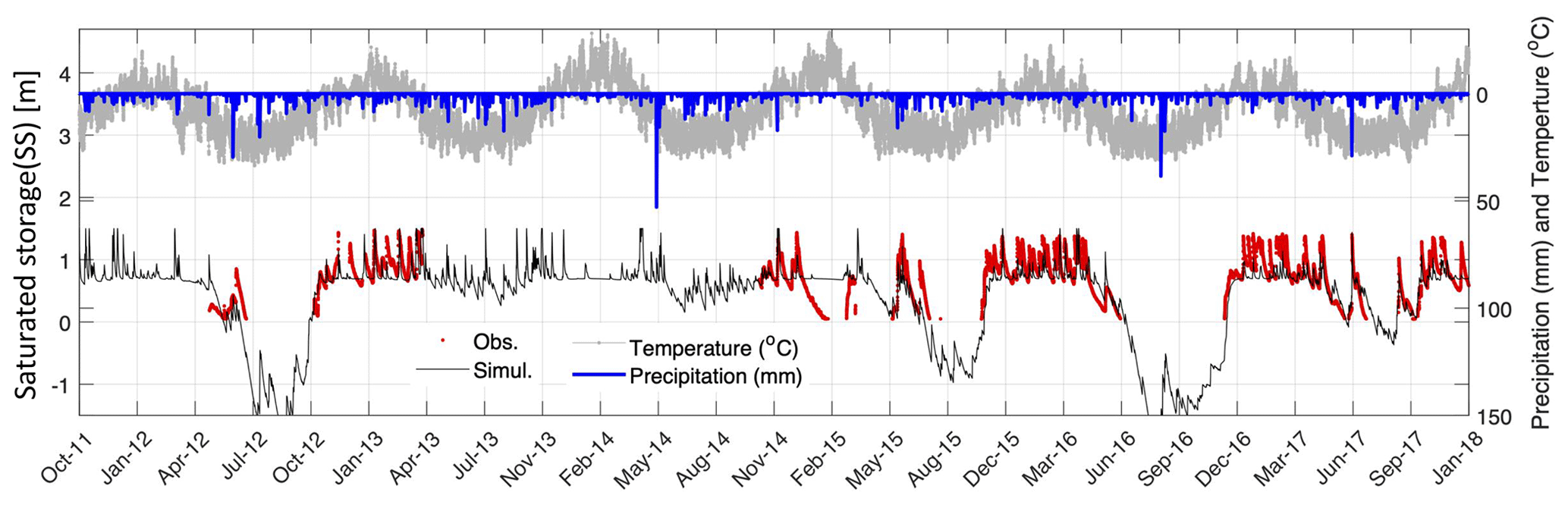
Figure 5 Time series of the simulated and observed saturated storage in the soil or groundwater layers of the model along with the observed temperature and precipitation.

Figure 6 Observed and simulated cumulative surface flow (a) and total flow (b).

Results show that tile flows generally occurred during snowmelt events, as indicated by the synchrony between snow water equivalent (SWE) depletion and tile flow. The maximum snowpacks (or snow water equivalent, SWE) were markedly smaller during the winters of 2016 and 2017 when compared with those of 2013 to 2015. However, this did not necessarily translate into lower tile flows as precipitation also occurred as rain during these seasons. Although peak tile drainage flow was not always predicted accurately, the model was able to capture the annual trends of both an absence of tile flow during the summer months (growing season) and the ascending and descending limbs of the tile hydrograph during events (Fig. 4).

3.2 Soil-saturated storage

Simulated and observed soil-saturated storage are compared in Fig. 5, alongside air temperature and precipitation observations. Despite the gaps in the observational record during two periodic equipment failures, the model agrees well with observations. Above tile drains, fluctuations in saturated storage were controlled by infiltration/recharge, tile flow, groundwater flow and matric potential that affect the drainable water from the capillary fringe. This caused flashier storage responses above the tile that were captured well by the model. In contrast, tiles did not withdraw water from the soil layer below the tile pipe and thus did not control fluctuations in saturated storage when levels were below the drain pipe, and tile drains did not flow during such periods. During the growing season, both the observed and simulated saturated storage dropped abruptly because of the seasonal lowering of the regional groundwater water table. In the growing seasons of 2012, 2015 and 2016, which were dry years, large declines in saturated storage were observed, whereas in wetter years such as 2013 and 2014 seasonal saturated storage declines were smaller. The seasonal declines in saturated storage during the growing season led to a cessation in tile flow in most years (Figs. 4, 5), even following rainfall events. For example, there was a large precipitation event (∼35 mm) in the growing season of 2016 that did not produce tile flow (apparent in both model and observations).

3.3 Surface flow and total flow

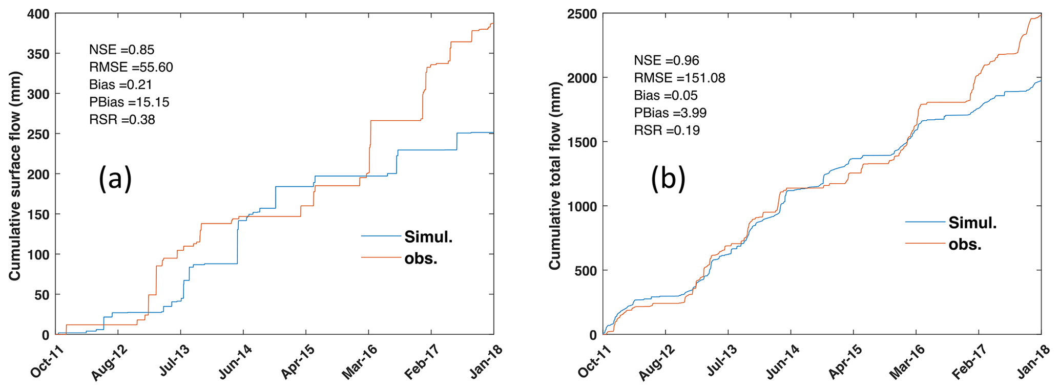
The model was not always able to capture the observed surface flow as satisfactorily as it captured tile drainage (Fig. 6a). Some possible reasons are uncertainties in the measurements of surface flow due to ponding in surface depressions on the field, which impeded the drainage of some of the surface runoff prior to exiting the field through the culvert (see Fig. 1), or uncertainty in field estimates of SWE. However, the model performance improved considerably when both runoff and tile flow were combined (referred to as total flow, Fig. 6b). Indeed, most of the flow from the field was through tile drains (80 % in 5-year average) rather than surface runoff (20 % in 5-year average) (Plach et al., 2019). The underestimation of both cumulative total and surface flows during 2017 and 2018 is possibly due to the removal of the blockage in the tile pipe in early 2017, which may have affected both surface and tile flow. The differences in timing of the simulated and observed surface flow for many of the main events (Fig. 6) shows that there remain systematic issues in simulation of surface flow by CRHM which should be addressed in future research.

3.4 Overall model performance

The model performance was calculated based on hourly data for various model outputs (Table 2). To compare the performance of the model in different seasons, we calculated the coefficient for entire year as well as separately for the growing and non-growing seasons. The results confirm that the model is robust over an annual cycle in the sense that it can capture the main patterns of tile flow, surface flow and saturated storage. The PBias values are below 25 % for most of the fluxes and cumulative fluxes. The RSR values are also generally below 1.0. The NSE values are positive and above 0.3 for most fluxes, except for surface flow, where the model exhibited some difficulties. The weaker performance of the model in the simulation of surface flow, which is illustrated by the NSE coefficient, can be partly related to difficulties in measurement of surface flow during flooding, ponding and freeze–thaw on the surface. The performance coefficients were calculated for the growing season, May–September (Table 2b), and non-growing season, October–April (Table 2c). The results show that surface flow biases are significantly larger and negative in May–September and are smaller and positive during October–April. For tile flow, the biases are slightly higher in May–September, whereas for saturated storage and total flow the biases are slightly lower in May–September. The NSE values are more acceptable in October to April for surface flow, tile flow and total flow, but the NSE for SS is more acceptable in May–September. The overall performance of the model for both tile and surface flow is more reliable in the non-growing season, when the regional water table was above the tile and saturated storage fluctuations were mainly controlled by tile flow rather than regional groundwater oscillations.

Table 2 Performance coefficients for surface flow, tile flow and saturated storage (SS), as well as total (tile + surface) flow, for the simulation period of October 2011 to January 2018. The coefficients were calculated for both hourly and daily flow rates for the whole year (a), for May to September (b) and for October to April (c) (green and red colours show that the seasonal coefficients improved and worsened, respectively, compared to their seasonal values).

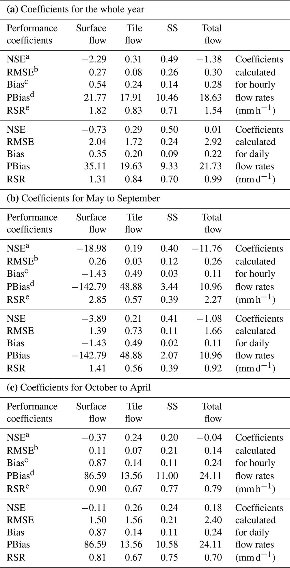
^a Nash–Sutcliffe efficiency. ^b Root-mean-square error. ^c Model bias.
^d Percentage bias. ^e RMSE-observation standard deviation ratio.

3.5 Presence of capillary fringe: effects and hypotheses

Results show that the thickness and vertical positioning of the capillary fringe had a strong impact on the amount of drainable soil water that flowed into the tiles. To investigate this effect further, the response of tile flow and soil moisture to changes in the capillary fringe was examined. It should be noted that although this thickness may change slightly depending on the soil type and water retention curves (Skaggs et al., 1978), the model assumed a constant value given the field-scale nature of the simulations and myriad of processes contemplated. However, despite the simplification, the vertical positioning of the capillary fringe was still calculated and enabled a dynamic (time-dependent) calculation of the drainable soil water that was available for tile drainage over time.

Effect of capillary fringe on tile flow

Figure 7a relates the simulated normalized total cumulative tile flow (Q_tR, total tile flow divided by the total tile flow when there is no influence of capillary fringe) to capillary fringe drainable water (${\mathit{\phi }}_{\mathrm{cR}}={\mathit{\phi }}_{\mathrm{c}}/{\mathit{\phi }}_{\mathrm{s}}$) for two different φ_s values (0.045 and 0.125). The values were normalized (0–1 scale) for comparison purposes. As expected, the model indicates that tile flow increases with drainable water, but the relationship is non-linear, likely because as tile carrying capacity is exceeded more frequently there is more opportunity for groundwater seepage and evapotranspiration. The direct effect of φ_s (comparing the solid and dashed lines) on tile flow is small, because the amount of water that can effectively drain to the tile is controlled by the capillary fringe and the associated drainable soil water. Figure 7b looks at the impact of the capillary fringe thickness on tile flow. Here, the values are also normalized. Results show that Q_tR decreases with an increase in the capillary fringe thickness T_CFR as long as it remains below 1 ($T_{\mathrm{CFR}}=\frac{T_{\mathrm{CF}}}{D_{\mathrm{t}}}$, capillary fringe thickness divided by tile depth). For T_CFR larger than 1, the capillary fringe remains below the soil surface.. Beyond this point, increments in the capillary fringe thickness have no impact on tile flow because condition 1 has been reached (see Fig. 2), which essentially means that the capillary fringe has reached the soil surface. The match between the curves for two different φ_s values shows that the changes in φ_s do not influence the effect of normalized capillary fringe thickness and drainable water on normalized tile flow. In Appendix D, the sensitivity of cumulative tile flow and mean saturated storage to different parameters is shown along with general approaches for evaluation of the model parameters for new sites, the site with no tile flow and water table observations.

Figure 7 Comparison between normalized tile flow (Q_tR) and (a) normalized drainable soil water (${\mathit{\phi }}_{\mathrm{c}}/{\mathit{\phi }}_{\mathrm{s}}$) and (b) capillary fringe thickness (T_CFR) for different maximum soil saturation values (φ_s), by drawing the model prediction lines.

Effect of capillary fringe on soil moisture

Observations and simulations of saturated storage reveal a bimodal frequency distribution (Figs. 8 and 9, respectively) with peaks at 0.85 and 1.25 m depth, with the former corresponding to the influence of the tile pipe and the second peak reflecting that from the capillary fringe. The frequency distributions of the simulated soil saturated storage (Fig. 9) show a first peak that highlights the efficiency of the tile in removing soil moisture. In contrast, the second peak indicates a strong model response to differences in the capillary fringe thickness. It shows that when there is near-constant percolation from the bottom of the soil layer, the matric potential varies the greatest while it remains between the tile depth and the soil surface. While the saturated storage fluctuates faster and is more unstable within this range, it also remains there for shorter periods. This bimodal response tends to push the saturated storage layer below the tile. In Fig. 9, the first peak happens at 0.9 m depth where the tile pipe is located, and the second peak happens at the depth equal to capillary fringe thickness. In Fig. 9 the second peak is clearer for the capillary fringe thickness of more than 1000 mm. The first peak in the observed saturated storage frequency plot (Fig. 8) happened around 0.8 m, which almost matches with the tile depth. And the second peak happened at a depth of ∼1.2 m, which shows that the capillary fringe thickness should be around 1.2 m. But, to have a more reliable estimate for the capillary fringe, based on Fig. 8, data are needed at depths greater than 1.5 m.

The bimodal behaviour of the observed and simulated saturated storage demonstrated here provides an opportunity to quantify the thickness of the capillary fringe using continuously monitored saturated storage. The capillary fringe thickness determined using this method can then be used as an input to the TDM module.

Figure 8 Histogram of the observed saturated storage distribution for the period of 2011 to 2018 in LON (Londesborough).

Figure 9 Histograms of the simulated soil-saturated storage versus saturated storage depth for the capillary fringe thicknesses of 0 (a, b), 400 (c, d), 800 (e, f), 1000 (g, h) and 1400 (i, j) mm and for the φ_s and φ_c of 0.125 and 0.025 (a, c, e, g, i) as well as 0.045 and 0.009 (b, d, f, h, j).

4 Discussion

4.1 Insights into key control mechanisms of tile flow for model simulations

The model suggests that tile flow may not be accurately predicted exclusively based on the soil's saturated storage and saturated hydraulic conductivity as suggested by the steady-state flow assumptions of Hooghoudt's equation (Hooghoudt, 1940). These results indicate two additional controls: (1) the amount of drainable soil water in the soil, which has also been identified in some field studies (e.g., Skaggs et al., 1978; Moriasi et al., 2013), and (2) fluctuations in saturated storage that are important to account for in simulations. However, the relationship between drainable water and tile flow rates is non-linear, as demonstrated in Fig. 7a. This is because the residence time for groundwater seepage and evapotranspiration increases when the hydraulic tile carrying capacity is exceeded. Comparatively, the effect of soil drainable water, φ_s (see also Fig. 7a), on tile flow is small, because the capillary fringe and associated drainable soil water control the amount of water that can effectively flow to the tile.

The verification of the model also indicated that the slopes of the rising and falling limbs of tile flow hydrographs and saturated storage were very sensitive to (1) the ratio between K_s and drainable soil water and (2) the net outflow in the soil through tile flow and fluctuations in saturated storage. This is supported by previous studies showing rapid responses of tile flow to precipitation events (Gentry et al., 2007; Smith et al., 2015) and others that have related rapid responses in tile discharge to antecedent moisture conditions (Macrae et al., 2007; Vidon and Cuadra, 2010; Lam et al., 2016a; Macrae et al., 2019), which can be affected by the development of a capillary fringe and its non-drainable water.

Results show that large fluctuations in saturated storage and tile flow during the cold season, when the water table tends to be above the tile, are primarily triggered by the development of a capillary fringe that reduces the amount of drainable soil water. Model sensitivity tests showed that a small amount of drainable soil water produces steeper rising and falling responses (and with larger fluctuation amplitudes) in both the saturated storage and the tile flow. Indeed, this pattern can be observed by exploring differences in tile drain responses in clay loam soils with larger field capacities (and correspondingly smaller drainable water) and smaller hydraulic conductivity, which are more likely to experience pronounced oscillations (e.g., steeper rising and falling response curves) compared to tile drain responses of sandy soil, which is characterized by reduced capillary forces, lower field capacities (but correspondingly larger drainable water) and higher hydraulic conductivity. Notably, both model and observations of saturated storage reveal a bimodal (i.e., two peaks) frequency distribution when examined in relation to the tile depth and capillary fringe thickness (Figs. 8 and 9, respectively). The two peaks (i.e., most frequently observed saturated storage) correspond with (1) the depth of the tile pipe (0.75 m), which demonstrates the efficacy of the tile at rapidly removing excess soil water, and (2) the capillary fringe thickness (for the depths of 1.0 and 1.4 m) (Fig. 9g, h, i and j) beyond which the amount of drainable water above the water table significantly increases.

These findings align well with studies such as Lam et al. (2016a) that recorded soil moisture near saturation after tile flow had ceased, suggesting the development of a capillary fringe. Combined experimental and modelling studies, such as in Moriasi et al. (2013) and Logsdon et al. (2010), also discuss the impact of drainable soil water (“drainable porosity” or “specific water yield”) on tile flow and note that the drainable water is, in turn, dependent on the soil type, soil-water dynamic depth and water table depth. However, these studies did not explore the dynamic nature of the capillary fringe and its thickness relative to the soil column above in determining the transient amount of drainage soil water that will impact the saturated storage frequency distribution and tile flow differently over time (conditions 1 to 3; see Fig. 2). Herein, while a capillary fringe with a fixed thickness that is generally related to the soil properties was assumed, its vertical positioning was simulated dynamically, which allowed for determining the drainable soil water based on the evolution of pressure head corresponding to field capacity. Thus, the development of the TDM has provided a step forward in the modelling of tile drainage and suggests that in loam soils such as those at the study site, the effects of a capillary fringe on tile flow should be included. Soil moisture (soil unsaturated storage) measurements from the study site by Van Esbroeck et al. (2017) between November 2011 and May 2014 from depths of 10, 30 and 50 cm (using the EC-5 soil moisture smart sensor) showed that almost 90 % of the gravitational soil moisture drains out in 0.5 to 2.5 h. This suggests that the saturated storage and capillary fringe can reach an equilibrium condition within 1 h at this field site, enabling the use of a steady-state equation (Hooghoudt, 1940) to predict the dynamic behaviour of the water table fluctuations.

4.2 Importance of capturing seasonal patterns in saturated storage to improve tile flow predictions

The saturated storage changed dramatically between seasons, affecting soil moisture (both saturated and unsaturated storage in the soil) and tile flow patterns. Both observations and model results show that low-precipitation and higher-evapotranspiration rates tend to produce little tile flow during the growing season. These seasonal patterns in precipitation and evapotranspiration are accompanied by a reduction in soil moisture (both unsaturated and saturated) that leads to a substantial storage capacity in fields. Even following moderate and high-intensity storms during the growing season, rapid soil moisture increases were observed (both saturated and unsaturated soil storage); however, tile flow rarely developed due to higher evapotranspiration and a seasonal decrease in the saturated storage, suggesting that the soil is able to hold the water (Lam et al., 2016a; Van Esbroeck et al., 2016). In contrast, tile flow was often observed during the cold season, with significantly smaller evapotranspiration fluxes, even during smaller rainfall–runoff and snowmelt events because of reduced soil storage but also a seasonal increase in regional groundwater table (Lam et al., 2016a; Macrae et al., 2007, 2019; Van Esbroeck et al., 2016). This concurs with several studies throughout the Great Lakes and St Lawrence region that have reported stronger tile responses during the non-growing season, with the summer months often showing little to no tile flow (Lam et al., 2016a, b; Jamieson et al., 2003; Macrae et al., 2007; Hirt et al., 2011; King et al., 2016; Van Esbroeck et al., 2016; Plach et al., 2019).

These results (the controlling effect of soil drainable water and saturated storage fluctuations on tile flow) suggest that while soil moisture (both saturated and unsaturated storage) is largely controlled by tile flow rather than saturated storage in the cold season, this reverses in the growing season (i.e., soil moisture controls tile flow), with soil moisture (both saturated and unsaturated storage) being also impacted by evapotranspiration. The controlling effect of groundwater fluctuations in the growing season has also been studied by Hansen et al. (2019). The model indicated that the rapid drops in observed saturated storage during the growing season could not be explained by evapotranspiration alone, thus pointing to the role of saturated storage. Johnsen et al. (1995) and Akis (2016) also showed that the effect of groundwater accretion was more effective on tile flows than surface runoff. Also, Vaughan et al. (1999) found that tile drain flows in their study site in the San Joaquin Valley of California were better explained and related to non-local groundwater appearance than to local variations in irrigation amount, evapotranspiration, variation in water storage or tile drain blockage. Thus, it was determined that in addition to soil-saturated hydraulic conductivity and soil thickness, the seasonal fluctuations in saturated storage and capillary fringe drainable water are other important controlling factors on tile flow rates.

5 Conclusions

A new tile drain module within the modular Cold Regions Hydrological Model (CRHM) platform has been created and tested at the field scale to support the management of agricultural basins with seasonal snow cover. The model was tested and validated for a small working farm in southern Ontario, Canada, and presents a step forward in the dynamic simulation of tile flow and its effects on the hydrological cycle in cold climates. Observations and model results showed that the dynamic prediction of tile flow and soil moisture at catchment scales needs to account for (1) the amount of drainable soil water that can be affected by the development of a capillary fringe and (2) fluctuations in saturated storage, in addition to (3) the typical saturated storage near the tile pipe depth and (4) the soil saturated hydraulic conductivity considered by the steady-state flow Hooghoudt's equation. The saturated storage and matric potential changed dramatically between seasons, affecting patterns of overall soil moisture and tile flow. Observations and model results showed that low-precipitation and higher-evapotranspiration rates caused minimal tile flows during the crop-growing season. Conversely, tile flow was often observed during the cold season, even during small rainfall–runoff and snowmelt events, due to a seasonal increase in soil-saturated storage.

Model sensitivity tests showed that the capillary fringe strongly affected the amount of drainable soil water flowing into the tile. Tile flow increased with drainable water, but the relationship is highly non-linear likely because, as the tile carrying capacity is exceeded more frequently, there is more time for groundwater seepage and evapotranspiration. Finally, observations and model results reveal a bimodal saturated storage response in the presence of tiles, which is controlled by the relative positioning of the capillary fringe in relation to the soil surface and the depth of tile drains below the soil surface. Capturing these dynamics is a critical advance, enabling the accurate prediction of the swift hydrological changes caused by the presence of tiles in models.

The TDM was developed as a first approximation from a single field site with the goal of providing insight into control mechanisms of tile flow. Given this limitation, it is not yet widely applicable across multiple field sites and for larger areas. Yet, the development of this module provides critical insights into its potential and performance for hourly time-step simulations, as well as the importance of saturated storage fluctuations and simplifying the capillary fringe parameters within models in some landscape types. Future work should build on the current model adapting it to different soil textures, such as those in clay loam soils, where preferential flow can have a strong impact on saturated storage and tile flow. Also, explicit representation of unsaturated flow may be needed to enable the use of the model in regions where groundwater is disconnected from surface water, as commonly happens in arid and semi-arid regions. Subsequent steps should also include the integration of the new TDM with CRHM's frozen soil and water quality modules.

Appendix A

Table A1 Instrument names and descriptions.

Appendix B

Table B1 Parameter names and their symbols in the CRHM platform.

Appendix C

Here, it is shown how seasonal factors (f_y,i) are assessed for different years. Equation (4) can be written as

$$\begin{array}{}\text{(C1)}& G_{y,i}=G\times f_{y,i}.\end{array}$$

For each year (y), f_y,i for the first (f_y,1) and second (f_y,2) part of the sine function (G) were assessed individually. In the first and second parts of the sine function for each year, it should be noted that G is larger than zero (G≥0) and smaller than zero (G<0), respectively. G can be defined for the two parts as

$$\begin{array}{}\text{(C2)}& \left\{\begin{array}{l}\mathrm{if}G\ge \mathrm{0}\left[i=\mathrm{1}\right]\mathrm{then}{f}_{y,\mathrm{1}}=x,\\ \mathrm{if}G<\mathrm{0}\left[i=\mathrm{2}\right]\mathrm{then}{f}_{y,\mathrm{2}}=y.\end{array}\right.\end{array}$$

G is the sine function representing the annual fluctuations in saturated storage (SS), or it can be simply defined as the percolation rate (in mm h⁻¹) of soil water to groundwater through lower semi-permeable layer. So, for n years there are $n\times \mathrm{2}{f}_{y,i}$ values. The default values for f_y,i are 1, and the default values can be changed for each year and for the first and second parts in each year independently. Calculating G_y,i in each time step add or subtracted to or from the total soil moisture depends on its sign. The f_y,i values for the sine function parameters are presented in Fig. C1. The verified sine function time series along with time series of temperature, precipitation and calculated evapotranspiration are shown in Fig. C1. In this figure it is obvious that in years 2012 and 2015 to 2017 the warm season amplitudes are larger. The evapotranspiration values are happening more in the warm seasons (growing seasons). Also, the seasonal oscillation in the sine function is very similar to the general temperature oscillations.

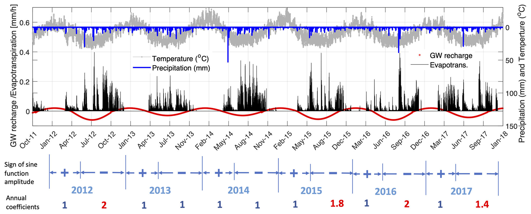
Figure C1 Time series of the adjustable sine function along with the time series of calculated evapotranspiration, temperature and precipitation during the study period from October 2011 to September 2018.

Appendix D

A sensitivity analysis was conducted for the cumulative tile flow (Q_tc), mean soil-saturated storage (SS) (it is equal to water table elevation, WT, as it is mentioned in Eq. 3) and cumulative outflow rate from the semi-permeable layer at the bottom of the soil to groundwater (G_c) (see Sect. 2.4.5, Eq. 4) with respect to six module parameters. Additionally, an approach for assessing model parameters at new sites, potentially lacking water table elevation and tile flow observations, is proposed.

D1 Sensitivity analysis

In this section, the sensitivity of Q_tc, SS and G_c to six distinct module parameters (namely capillary fringe thickness (T_CF), capillary fringe drainable water (φ_c), soil-saturated hydraulic conductivity (K), soil thickness (T_SL), sine function amplitude (A) and sine function (B)) was examined. Q_tc, G_c and SS were computed over the entire simulation period (expressed in units of mm, mm and m, respectively). Figure D1a to f illustrate these sensitivities, with each parameter's impact discussed in dedicated sections.

D1.1 Sensitivity to capillary fringe thickness

To gauge sensitivity to capillary fringe thickness T_CF, flow rates and the SS were analyzed for T_CF ranging from 0 to 1600 mm. Figure D1a indicates that as T_CF increases, both cumulative tile flow (Q_tc) and mean soil-saturated storage (SS) decline. The SS drop is sharper for T_CF beyond 900 mm. Beyond this thickness, Q_tc stabilizes at a minimal value. A negative SS indicates its position below the tile pipe. G_c remains consistent despite T_CF variations.

D1.2 Sensitivity to capillary fringe drainable water

With rising φ_c, both Q_tc and SS surge (Fig. D1b). As φ_c ascends from 0.005 to 0.45, Q_tc jumps from 1300 to 1900 mm and SS jumps from −0.45 to −0.25 m (Fig. D1b). G_c stays constant, irrespective of φ_c fluctuations.

D1.3 Sensitivity to soil hydraulic conductivity

Increasing soil hydraulic conductivity (K) from 0 to 10 mm h⁻¹ leads to a surge in Q_tc and a drop in SS (Fig. D1c). However, adjusting K from 10 to 50 mm h⁻¹ results in levelling off slopes for Q_tc and SS, especially when K>20 mm h⁻¹. Both metrics are acutely responsive to K when K is below 10 mm h⁻¹ but become non-responsive beyond 20 mm h⁻¹. The G_c response to K remains neutral.

D1.4 Sensitivity to soil thickness

Similar to K, a rise in T_SL from 1500 to 15000 mm causes Q_tc to rise and SS to decline (Fig. D1d). The most significant rate of change for both metrics occurs between 1500 to 5000 mm T_SL. Beyond 5000 mm, changes flatten. G_c shows no response to T_SLvariations.

D1.5 Sensitivity to sine function amplitude

Increasing the sine function amplitude, A, from −0.03 to 0 mm h⁻¹ pushes both Q_tc and SS to increase and reach their maximum at A=0 (Fig. D1e). But as A rises from 0 to 0.06 mm h⁻¹, they both decline. In contrast, G_c descends to its lowest (400 mm) when A shifts from −0.03 to 0 and then increases to 900 mm as A hits 0.063.

D1.6 Sensitivity to sine function intercept

Both Q_tc and SS ascend with the growth in the sine function's intercept, B. Increasing B from −0.015 to 0.005 mm h⁻¹ sees G_c descend. During this B increase, Q_tc expands from 1100 to 2400 mm, while G_c shrinks from 1400 to 0 mm. It seems the sum of Q_tc and G_c might be constant. This suggests that water either drains through the tile pipe or percolates through the soil bottom.

Q_tc and SS appear sensitive to all six module parameters, but G_c is only sensitive to A and B.

D2 Module parameter evaluation for new sites

As discussed in Sect. 2.5, initial values for K, T_CF and φ_c can be determined by the soil grain-size distribution. Parameters less explored in past research for new sites include the sine function's amplitude (A), intercept (B) and time delay (D_d).

D2.1 Evaluating the sine function's A and B

If no percolation exists from the soil's bottom to groundwater and G_y,i is zero, both A and B should be zero. However, if percolation or interactions between soil and groundwater occurs, A and B need calibration assessment. Before this, reasonable initial values and bounds must be set.

From this study's findings, A and B should fall between the mean hourly difference of infiltration and observed tile flow rates. For instance, observed hourly rates for infiltration and tile flow at our site are 0.07 and 0.03 mm h⁻¹. Thus, A and B initial values should range from −0.04 to 0.04 mm h⁻¹. Negative A and B values indicate outflow from soil to groundwater and vice versa. Initial values were set at 10 % of the range limits: −0.004 for B and 0.004 for A. Eventually, B and A were adjusted to −0.005 and 0.025 mm h⁻¹.

D2.2 Assessment of the sine function's time delay

The sine function begins on the first Julian day. If its peak occurs around the 91st Julian day (3 months later), its minimum should be on the 274th day. If the peak comes later, say the 111th day, a 20 d delay is present. This delay should mirror in both function's minima and maxima. In this case, the minimum would be on day 294. This delay aligns with the soil water table's peak annual fluctuations. When no observed fluctuations exist, the delay can be calibrated. A sensible initial delay can be ascertained by examining the study site's water table elevations, fitting a sine function and noting the peak's Julian day annually.

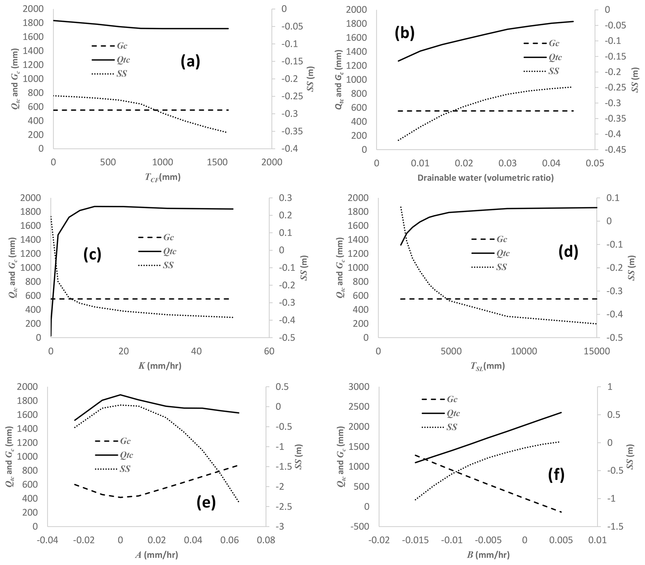
Figure D1 Sensitivity of cumulative tile flow, Q_tc; cumulative soil to groundwater percolation rate, G_c; and mean soil-saturated storage elevation, SS; to capillary fringe thickness, T_CF (a); capillary fringe drainable water, φ_c (b); soil hydraulic conductivity, K (c); soil thickness, T_SL (d); sine function amplitude, A (e); and sine function intercept, B (f).