the Creative Commons Attribution 4.0 License.
the Creative Commons Attribution 4.0 License.
 | 14 Jun 2024
Climatology of snow depth and water equivalent measurements in the Italian Alps (1967–2020)
Roberto Ranzi
Giorgio Galeati
A climatology of snow water equivalent (SWE) based on data collected at 240 gauging sites was performed for the Italian Alps over the 1967–2020 period, when Enel routinely conducted snow depth and density measurements with homogeneous methods. Six hydrological sub-regions were investigated spanning from the eastern Alps to the western Alps at altitudes ranging from 1000 to 3000 m a.s.l. Measurements were conducted at fixed dates at the beginning of each month from 1 February to 1 June and on 15 April. To our knowledge, this is the most comprehensive and homogeneous dataset of measured snow depth and density for the Italian Alps. Significant decreasing trends over the years at all fixed dates and elevation classes were identified for both snow depth, equal to −0.12 ± 0.06 m per decade, and snow water equivalent, equal to −51 ± 37 mm per decade, on average in the six macro-basins we selected. The analysis of bulk snow density data showed a temporal evolution along the snow accumulation and melt season, but no altitudinal trends were found. A Moving Average and Running Trend Analysis (MARTA triangles), combined with a Pettitt's test change-point detection, highlighted a decreasing change of snow climatology occurring around the end of the 1980s. The comparison with winter temperature and precipitation data from the HISTALP dataset identified a major role played by temperature on the long-term decrease and changing points of snow depth and SWE with respect to precipitation, mainly responsible for its variability. Correlation with climatic indexes indicates significant negative values of the Pearson correlation coefficient with winter North Atlantic Oscillation (NAO) and positive values with winter Western Mediterranean Oscillation (WeMO) for some areas and elevation classes. Results of this climatology are synthesized in a temporal polynomial model that is useful for climatological studies and water resources management in mountain areas.
- Article
(6740 KB) - Full-text XML
-
Supplement
(11549 KB) - BibTeX
- EndNote


The effects of global climate change on the cryosphere at different latitudes have been widely studied in the last decades (IPCC, 2019). The comparison between photos of the past decades with the current ones, together with imagery analysis from satellites, confirms the retreat of glaciers in the Alpine region (Ranzi et al., 1999; Beniston, 2012). Analysis of long-term observed snow depth and simulated bulk snow density in 20 gauging sites in the Italian Alps highlights a decrease in snow water equivalent especially after the 1990s (Colombo et al., 2022). Modifications of the greater Alpine region climate have been confirmed by the analysis of the HISTALP dataset, with significant trends in temperature (twice as the global average), precipitation and (in low elevation areas) relative humidity (Auer et al., 2007; Brunetti et al., 2009). In fact, the Alpine region is an extremely sensitive area to the variations in climate conditions, making mountain glaciers sentinels of climate change.
Snow is the largest component of the cryosphere in terms of areal extension. Its importance in the Alpine region is related to climatological, hydrological, biological, economic and social aspects (Beniston et al., 2018). Snow cover regulates the surface energy balance, affecting circulation patterns and atmospheric flow regimes (Gong et al., 2004; Ge and Gong, 2009). The hydrological cycle is strongly dependent on the separation between solid and liquid precipitation and the timing of the melting season onset, mainly driven by temperature, and the hydrological response of high-mountain catchments is often regulated by snowmelt and accumulation (Penna et al., 2016). Moreover, snow accumulation and melting are major components of the mass balance of glaciers. Snow monitoring is crucial in order to provide a proper estimate of glaciers mass and energy balance to evaluate glacial response to snow cover variations (Ranzi et al. 2010). The presence of snow is also of paramount importance for ski resorts and for winter tourism in general in the Alpine region, accounting for about EUR 10 billion, maintaining seasonal jobs and slowing down the rural depopulation in the valleys (Lehr et al., 2012; Reynard, 2020). The water stored as snow in winter is released as the melting season begins, contributing to the water availability for agriculture and energy production in hydropower plants (HPPs).
Hence, it is of great interest for HPP managers to have an accurate quantification of the snow water equivalent (SWE) and possible variability in a climate change scenario (Schaefli et al., 2007). In view of this, since 1966, Enel (former Italian national electricity board) has conducted systematic observations of snowpack depth and density in the basins subtended by seasonal regulation reservoirs (Berni and Giacanelli, 1966). The Enel measurement program is similar to other institutional measurement networks (e.g., SNOTEL; Serreze et al., 1999). Before the creation of Enel, some power companies already took care of periodic measurements of the snowpack consistency on the Alpine and Apennine basins supplying reservoirs within their competence. However, these surveys were carried out unevenly, adopting different instruments and, of course, with different procedures for processing and interpreting the collected dataset. The Enel measurement campaigns were scheduled since the early 1960s at fixed dates from 1 February to 1 June at fixed locations in the catchments of the main Alpine reservoirs. Such an extensive and standardized monitoring campaign represents a rich and valuable source of in situ measurements covering a wide portion of the Italian Alps for a 54-year time window spanning the 1967–2020 period. Hydrological models and remote sensing techniques have been widely used to estimate SWE (Taschner et al., 2004; Tedesco et al., 2015) and snow cover (Terzago et al., 2010). However, in situ measurements are required to validate such estimates, and it is not trivial to reconstruct a coherent time series long enough to be suitable for climatological studies by means of satellite observations. Lejeune et al. (2019) used a snow dataset of 57 years from a mountain meteorological station to evaluate snow depth variability between 1960 and 2017, a temporal range sufficiently wide enough to evaluate climate impacts on snow depth. A similar dataset has been used by López-Moreno et al. (2020) to evaluate long-term trends of snow depth and snow cover in the Pyrenees. Schöner et al. (2019) used an ensemble of 196 stations to study the snow depth and its linkages to climate change over the Swiss–Austrian Alps over the monitoring period of 1961–2012. A more comprehensive study of the Northern Hemisphere has been carried out by Pulliainen et al. (2020) using the GlobSnow v3.0 dataset (Takala et al., 2011) for the monitoring period of 1980–2018. Valt and Cianfarra (2010) found a reduction of snow cover duration and snowfall between 1950 and 2009, together with breakpoints of the time series at the end of the 1980s. Marty et al. (2017) observed a SWE decrease, more pronounced in spring than in winter, over the observation period of 1968–2012. Colombo et al. (2022) modeled the SWE from 19 historical snow depth measurements and studied the links of the Standardized SWE Index with teleconnection indexes and temperature anomalies. Marcolini et al. (2017) analyzed snow depth series in the Adige basin, finding a reduction of snow cover duration and snow depth over the period 1980–2009, especially at low-elevation sites. The dataset we use here covers almost the same period of previous studies, but it is spatially distributed over the Italian Alpine region and includes bulk snow density measurements to estimate SWE. Such a combination of spatial and temporal coverage makes this dataset an extremely precious support to understand snow variability and climate change impacts in the Italian Alps. Unlike previous studies, we make use of not only measurements of snow depth but also extended observations of bulk snow density, instead of modeled estimates, over a very long period and a wide spatial coverage of the Italian Alps. The novelty also relies on the homogeneity of the data collection methods of SWE measurements conducted for purposes of hydropower generation management.
In this study, we present a detailed long-term trends and variability analysis of snow depth and SWE measurements in a wide portion of the Italian Alps between 1967 and 2020. The first objective of this research is to quantify how snow depth and SWE has changed in time over the monitoring period, evaluating temporal trends and identifying possible change points using an unprecedented dataset. The second objective is to establish elevation and seasonal dependencies of snow depth and snow density. A large dataset covering a wide area and spread at different elevations, like the one presented here, is suitable for such considerations and for fitting simple models able to describe those dependencies, with the aim of obtaining a climatological estimate of SWE as a function of the day of the year and altitude. The third objective is to understand the links between meteorological variables with snow depth and SWE. In particular, we aim to better understand what are the weights played by temperature, precipitation and teleconnection indexes.
In Sect. 2, after a description of the study area and the snow depth and density measurement procedure, we present the datasets adopted and describe the statistical methodology used for the climatological analysis, together with a simple model to estimate the SWE as a function of elevation and day of the year. In Sect. 3, we present and discuss the results obtained for the climatological analysis of snow depth, bulk snow density and SWE, the comparative analysis of meteorological variables and climatic teleconnection indexes, and, finally, the estimates of SWE obtained with the presented regression model.
2.1 The study area and basin aggregation
In this study, we focus our analysis on the following basins of the Alpine region: Cordevole and Piave in the Veneto region; Cismon, Brenta, Noce, Sarca, Chiese, and Valsura in the Trentino-Alto Adige/Südtirol region; Mallero, Adda, Bitto, Serio, Brembo, and Oglio in the Lombardia region; and Toce in the Piemonte region. We aggregate the individual basins into six groups (Fig. 1a) according to the hydrographic criteria, merging tributaries to the main river branch (e.g., Cordevole aggregated to Piave), and the geo-morphoclimatic criteria, aggregating basins with similar annual average precipitation, temperature and geographical orientation (e.g., Piave and Brenta or Oglio, Chiese, and Sarca). Measurements aggregation is a crucial step in the analysis and implies a change of scale (Blöschl, 1999). However, we believe that the adopted data aggregation can be representative of the selected macro-basins.
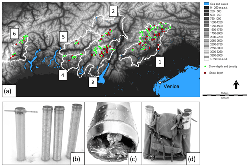
Figure 1(a) Map of the research area. The individual basins are grouped into six macro-basins by number: (1) Piave-Brenta, (2) Adige, (3) Oglio-Chiese-Sarca, (4) Serio-Brembo, (5) Adda and (6) Toce. Locations of snow depth and density (green dots) and snow depth (red squares) are also reported. (b) Photo of the CN2-type snow sampler, (c) details of the cutting knife with the three internal fins and (d) the complete kit in its transporting bag.
Toce basin's slopes are mainly oriented east, and its climate is affected by the influence of Lake Maggiore. As it is the only basin where data are available in the Piemonte region, we decided not to aggregate it with other basins (we denote the group simply as Toce). Since Serio and Brembo are the tributaries of the lower Adda, downstream of Lake Como, and their slope is mainly oriented southward, facing the Po River valley, they can be grouped into a unique macro-basin denoted as Serio-Brembo. Bitto and Mallero slopes are facing north and south, respectively, and both basins are tributaries of the upper Adda, oriented westward, upstream of Lake Como. Consequently, we aggregate Bitto, Mallero and Adda basins into one group (denoted as Adda). Oglio, Chiese and Sarca basins are fed by meltwater of the Adamello glacier; accordingly, we considered a unique macro-basin called Oglio-Chiese-Sarca. We denote Adige as a macro-basin including its tributaries Noce and Valsura. Finally, we aggregate Piave, Brenta, Cismon and Cordevole into another group (denoted Piave-Brenta), which is most influenced by the Adriatic Sea. The main characteristic of the macro-basins, such as the catchment area and minimum, maximum, and average elevations, are reported in Table 1.
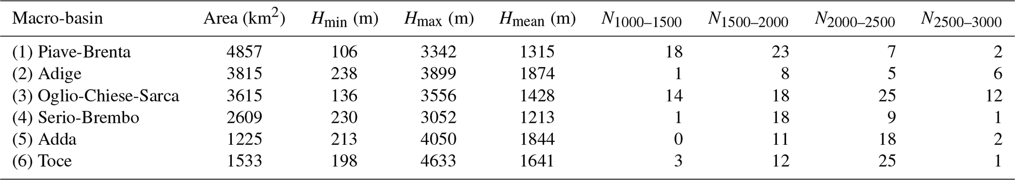
Table 1Area and minimum, maximum, and mean elevations of the considered macro-basins. For each macro-basin, the numbers of snow depth measurement points by elevation class are given.
2.2 Snow depth, snow density and snow water equivalent
We use a dataset of snow depth and bulk snow density measurements collected between 1967 and 2020. The locations of the measurement stations, reported in Fig. 1a, are fixed with minor displacements over the monitoring period. For each measurement station, multiple measurements of snow depth were taken and then averaged. The choice of such locations is based on accessibility in every moment of the winter under normal meteorological conditions and representativeness of natural snow deposition, avoiding areas where avalanche snow might be collected or places where other forcings might change the snowpack height. The measurement dates are fixed in time on 1 February, 1 March, 1 April, 15 April, 1 May and 1 June, providing strong consistency for the time series analysis.
The tools adopted for height and density measurements of the snowpack have been designed by the Hydrographic Office of the Water Authority of Venice. One of the tools is a CN2-type snow sampler (Fig. 1b), derived from the CN1 type, tested by the Snow Commission of the Glaciological committee through small technical changes suggested by Enel in order to make use of it easier and faster. The CN2-type snow sampler is made of four tubular elements in duraluminium, each 50 cm long and with an internal diameter of 7.2 cm. Screwable brass caps are attached to the ends of the four tubes, allowing users to join two or more elements. On the side of each tube there are measurement notches from 0 to 50 cm in order to measure the exact height of the snow. The checking of this height is completed with a graduated rod, made of three plugable elements in a rust-proof alloy. Other accessories that complete the snow weighing toolset are two snow-cutting knifes (Fig. 1c) attachable to the bottom of each of the duraluminium tubes with three internal fins designed to prevent the loss of snow at the bottom, dynamometers for the weighing, a shovel for digging the trenches, nylon bags with rings to attach the dynamometers, and a hammer and wrenches for screwing the tubes (Fig. 1d). In recent years, in some sites, the probes were substituted with Teflon probes with similar characteristics.
The measurement procedure of snow depth and density in the case of snowpack height lower than 2 m starts with a first check of the snow depth with a graduated rod in order to prepare the instrumentation with the proper number of tubular elements. Then, the instrument is thrust into the snowpack, applying a constant pressure and continuous rotational movement until ground level and reading the snow depth measurement on the external notches. Finally, the instrumentation is extracted from the snowpack, depositing the collected sample in a nylon bag to be weighed. In the case of snowpack deeper than 2 m, multiple extractions are necessary. A snow pit must be dig up to ground level, paying attention to maintain the front wall vertical. Then, an aluminum plate is inserted horizontally, a first sample is taken from the snowpack surface until the plate is reached, and the partial depth measurement is recorded. The procedure is then repeated until the ground level is reached. The bulk snow density is finally computed by dividing the weight by the known volume of the sample. In the case of the snow depth measurement only, a simple graduated rod is adopted.
Each snow depth and bulk snow density measurement is recorded together with the name of the drainage basin, average slope, orientation with respect to the north and elevation. We aggregated data into the six macro-basins described in the previous section in four elevation bands of equal range of 500 m (1000–1500, 1500–2000, 2000–2500 and 2500–3000 m a.s.l.). Overall, 44 411 snow depth and 14 479 bulk snow density measurements were collected and processed. Among the available 299 gauging sites, a subset of 240 stations located within the considered basins has been analyzed.
The spread and spatial density of the points of measurement exhibit differences in the distribution of the data between elevation classes (Table 1). The Oglio-Chiese-Sarca basin presents the largest number of observations of both snow depth and bulk snow density for all the elevation classes, followed by the Piave-Brenta basin, with similar measurement density for the three elevation classes between 1000 and 2500 m a.s.l. Accordingly, we expect more robust and representative results for these two areas. The Adige basin exhibits a good spread of snow depth measurements, except for the 1000–1500 class. In the Adda basin, snow depth and bulk snow density measurements are available only for the 1500–2000 and 2000–2500 elevation classes, with a slightly higher number of observations in the latter. For the Toce and Serio-Brembo basins, a similar numerosity of observations can be found in the same two middle elevation classes, with a higher number of measurements in the 1500–2000 class for Serio-Brembo and in the 2000–2500 class for Toce.
We performed a preliminary data quality check in order to remove possible erroneous data due to human mistake in the data recording. In the case of snow depth, it might happen that a zero is recorded instead of a missing value. Specifically, we checked all the zero snow depth records by comparing them with the closest measurement points. If the snow depth measurements in the locations nearby the equivocal point are larger than a fixed threshold (set at 0.7 m), we consider that zero as a missing value. In the specific case of equivocal measurements on 15 April, we also checked the previous and following dates of measurements at that point. If in that location the snow depth on 1 April and 1 May is larger than 0.7 m, we consider the equivocal zero as a missing value. In the case of bulk snow density measurements, we removed density values larger than a fixed threshold of 0.75 g cm−3, considered far larger than typical bulk snow density values (USACE, 1956; Marbouty, 1980).
We used the snow depth and bulk snow density measurements that have passed the quality check to compute the SWE (mm) as
where HS (mm) is the snow depth, ρs (kg m−3) the bulk snow density and ρw (kg m−3) is the liquid water density simply estimated as 1000 kg m−3. Since there is not a bulk snow density measurement for each snow depth record, we assigned to ρs the measured snow density only if present. In the case of a missing bulk snow density value in correspondence with the considered snow depth measurement, we assigned to ρs a mean value computed as the average of the other available snow density values measured in the corresponding date, macro-basin and elevation class. In the case that there are no density measurements in the corresponding geomorphic class, we consider the SWE data for the specific date, macro-basin and elevation class as missing. Finally, we obtained a time series ranging from 1967 to 2020 of average value snow depth and bulk snow density for each macro-basin, elevation class and measurement date.
2.3 Temperature and precipitation data
Precipitation and temperature are the main meteorological variables regulating accumulation and melting of snow, with air temperature mainly governing the separation of solid and liquid precipitation and driving snowmelt. To evaluate the effects of precipitation and temperature variability on snow depth and SWE in the considered macro-basins, we consider the HISTALP dataset (Auer et al., 2007; Chimani et al., 2011). HISTALP is a multi-century-long (1780–2015) database of monthly homogenized records of temperature, pressure, precipitation, sunshine and cloudiness for the Alps. Here, we consider the gridded precipitation and 2 m above ground level air temperature data, provided at 0.08° spatial resolution. Specifically, we considered the average temperature of December, January, February and March (DJFM) over the period 1967–2015. Since 1967, the number of the meteorological stations adopted to create the database and the distance between them have not changed (Auer et al., 2007), making the time series sufficiently reliable for the long-term variability and trend analysis. We extract from the gridded dataset the average temperature over each macro-basin reported in Fig. 1a. Accordingly, we consider the accumulated precipitation of December, January, February and March. These averaged time series do not take into account the altitudinal dependence of climatic variables, but they serve as a valuable indicator for assessing the average variability and trends of temperature and precipitation in the considered basins. Additionally, the use of the HISTALP dataset enables a consistent analysis across the six different basins.
2.4 North Atlantic Oscillation and Western Mediterranean Oscillation indexes
Following an approach widely adopted (Maragno et al., 2009; Bocchiola and Diolaiuti, 2010; Diolaiuti et al., 2012; Ranzi et al., 2021), we evaluate the link of SWE with large-scale circulation variability. Specifically, we consider the North Atlantic Oscillation (NAO) index and the Western Mediterranean Oscillation (WeMO) index. NAO is a global circulation pattern index defined as the normalized surface sea-level pressure difference over the North Atlantic Ocean between the subtropical (Azores) high and subpolar (Iceland) low. It influences the European climate during winter (Osborn, 2011), and it presents a negative correlation with precipitation in the Italian Alps (Steirou et al., 2017; Zampieri et al., 2017; Brugnara and Maugeri, 2019). The WeMO index is a regional teleconnection pattern, spatially limited to the western Mediterranean basin (Martin-Vide and Lopez-Bustins, 2006). It is defined by the difference of monthly sea-level pressure between the Padua and San Fernando (Cádiz) stations. Here, we consider average winter (DJFM) NAO and WeMO indexes to address the links with spring (April) snow depth measured in the considered Alpine basins. The comparison between winter teleconnections and April snow depth aims to investigate the impact of atmospheric circulation patterns on winter precipitation and snow accumulation, generally reaching maximum values in April.
2.5 Statistical and climatological analysis
In order to investigate possible variability and tendencies of snow depth and SWE during the monitored period, we adopt three main methods of statistical analysis. At first, we compute the trend over the complete period 1967–2020 by means of a least-square linear regression. To test the statistical significance (p value < 0.05) of such trends, we adopted the Mann–Kendall (MK) non-parametric test (Mann, 1945; Kendall, 1938) and the parametric Student's t test on the slope of the regression line, testing the null hypothesis H0 of no trend against the alternative hypothesis H1 of linear trend (Kottegoda and Rosso, 2008). Such a trend analysis provides only one piece of information, even if important, related to the general tendency of the studied time series. The second analysis consists of a Moving Average and Running Trend Analysis (MARTA from this point on), similarly to that reported in Brunetti et al. (2009) and Ranzi et al. (2021). MARTA consists of computing the running trend and a moving average for all the possible sub-periods longer than 10 years, reporting the results in a chart where the central year of the sub-period is reported on the horizontal axis and its length on the vertical one. In the chart of the running trends, computed by least-square linear regression, slopes are represented by the color of the pixel. We represent on the plot each trend. However, statistically significant trends according to the MK test (p value < 0.05) are represented by thicker pixels. In the chart of the moving averages, instead, all the sub-period averages are reported. MARTA is an effective exploratory data analysis and visualization tool, which is able to capture and highlight periods of values higher or lower than the long-term mean in the time series. Here, we extend the approach taken from Brunetti et al. (2009), including a change detection analysis by means of the application of Pettitt's test (Pettitt, 1979). Pettitt's test is a non-parametric technique to solve the change-point problem (i.e., identifying if and when the probability distribution of a stochastic variable has changed), testing the null hypothesis H0 of no change. We graphically represent the change point, if present, in the moving-averages chart, indicating the year detected with the statistical test. As a third analysis, to evaluate the global behavior of snow depth and SWE in each basin, we compute the difference between the averages of the two halves of the monitoring period (1967–1993 and 1994–2020). We test the statistical significance of such differences by means of the non-parametric Mann–Whitney U test (Mann and Whitney, 1947). In this case, we test the null hypothesis that the population of the sample of the measured variable in the period 1967–1993 is equal to the population of the sample of the measured variable in the period 1994–2020; the alternative hypothesis is that the second sample is stochastically smaller than the first sample (i.e., the cumulative distribution function (CDF) of the first sample P1(x) is larger than the CDF of the second sample P2(x) for every x). We divided the entire observation period into two equally long sub-periods such that the two samples of the considered variable could have the maximum possible number of observations to be sufficiently representative of each climatology. In fact, climatologies are generally assessed over periods lasting 30 years at least. With the available data, spanning 54 years, our subdivision enables us to analyze two independent periods with sufficient climatological significance. Another possible division of the monitoring period could be centered on the identified change point (if present and statistically significant). However such a division would introduce two major limitations in the analysis. First, one of the two sub-periods could be largely represented than the other. Second, we prefer to keep the Mann–Whitney U test results independent from those of the Pettitt test.
Finally, we study the relationship and dependencies of snow depth and SWE with variability and changes in climate. We perform the same MARTA for the temperature and precipitation time series presented above. Moreover, to evaluate the possible links between snow depth and the teleconnection indexes, we evaluated Pearson's correlation between the snow depth on 1 April and 15 April and the winter (DJFM) NAO, previously investigated by other authors (e.g., Colombo et al., 2022), and WeMO indexes, here firstly compared with the snow depth observation.
2.6 Mean snow climatology model
To compute the SWE, it is necessary to have a measurement of both snow depth and bulk snow density (USACE, 1956; Fierz et al., 2009). Empirical regressions of bulk snow density over day of the year in the Italian Alps have been studied by several authors (e.g., Sturm et al., 2010; Avanzi et al., 2015; Pistocchi, 2016; Guyennon et al., 2019). Accordingly, we evaluated the average temporal evolution of bulk snow density during the monitoring period, updating it with our new dataset and the parameters of the model proposed by Guyennon et al. (2019), who found that the temporal evolution of bulk snow density is well described by a quadratic polynomial function of the day of the year as
where ρs is the bulk snow density, DOY is the day of the year. The choice of a second-order polynomial formulation, following Guyennon et al. (2019), was made to include a term overcoming the assumption of a simpler linear model such as the one of Pistocchi (2016).
Snow depth on the ground increases during the accumulation season and starts decreasing after the melt onset. Concurrently, positive correlations between snow depth or SWE and elevation in the Alps are reported by many authors (Bavera and De Michele, 2009; Durand et al., 2009; Lehning et al., 2011; Grünewald et al., 2014). Accordingly, we propose a snow depth model that is linearly dependent on elevation and with time-dependent coefficients. For each macro-basin and measurement date, we estimate the best-fitting linear model of average observed snow depth as a function of elevation as
where hs (m) is the snow depth, H (m) is the elevation above sea level, m (–) is the slope and H0 (m) is the elevation of null snow depth in the regression (snowline elevation). In such way, we reconstruct the elevation dependency of snow depth at different times of the accumulation and melting seasons, starting from the 1 February and ending on the 1 June. Hence, the temporal dependency is contained in the coefficients m and H0, computed for each available measurement date. In order to obtain a continuous estimate of snow depth as a function of both elevation and time, we fit the computed m and H0 using a third-order polynomial curve as
where a0, a1, a2, a3, b0, b1, b2 and b3 are obtained by a least-square best-fitting procedure.
By substituting Eqs. (4) and (5) into Eq. (3) and then Eqs. (2) and (3) into Eq. (1), we obtained a simple model to estimate the SWE as a function of both elevation and time, expressed as
The parameters of the proposed model are calibrated for the two periods mentioned above (1967–1993 and 1994–2020) and for each macro-basin. Because of the scarcity of measurements above 2500 m a.s.l., it is not easy to determine whether a maximum threshold is reached at higher altitudes. Moreover, Grunewald et al. (2014) found that snow depth increases with elevation until a certain level. Considering that at higher altitudes the major slopes tend to trigger avalanches and that the blowing winds tend to prevent snow deposition, we assume, based also on the available observations, that our altitudinal trends for the investigated region can be extrapolated up to 2500 m a.s.l., and a plateau value can be assumed above such an altitude. Such a threshold is dependent on the topography of the considered basin and a larger number of high-elevation measurements is needed to provide a better estimate of the elevation of the plateau in other mountain ranges and climatic regions.
3.1 Snow depth
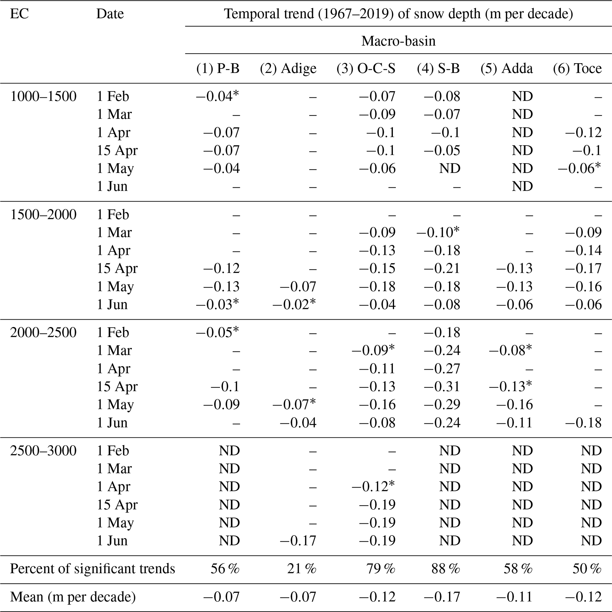
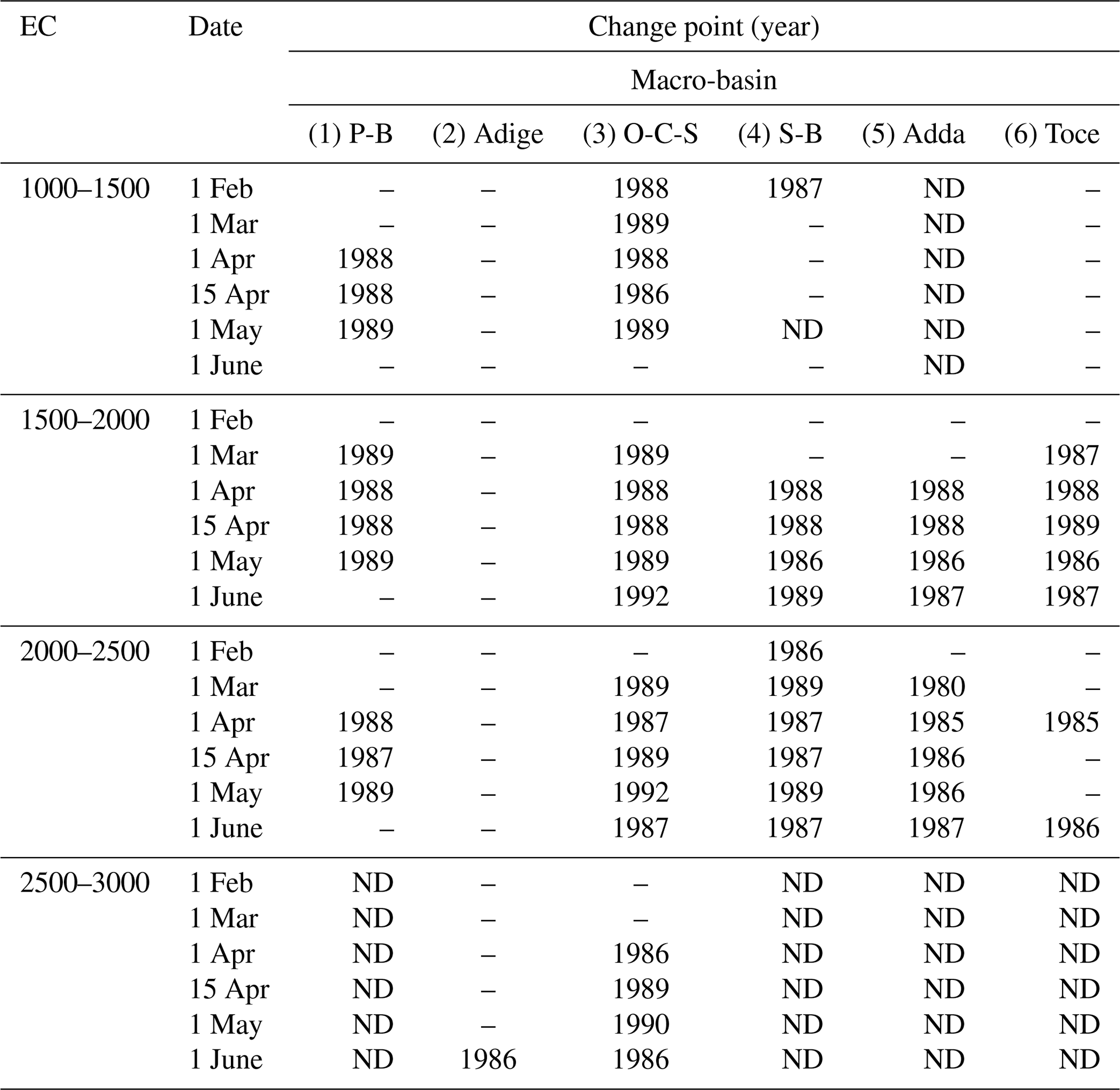
We computed the temporal trends of snow depth for each macro-basin, elevation class and date of measurement. In Fig. 2, we report the MARTA triangles of snow depth for the Toce and Oglio-Chiese-Sarca macro-basins on 1 April and 1 May. Such a graphical representation of the running averages and trends highlights the temporal variability of the time series analyzed. For each case, the snow depth time series shows a decreasing trend, with a slightly steeper regression line in the case of the Oglio-Chiese-Sarca region. We observe statistically significant decreasing trends for the Oglio-Chiese-Sarca basin for all the considered time spans, with the shorter windows centered around 1990. The results of long-term trends (1967–2020) for each macro-basin, elevation class and date of measurement are reported in Table 2. All the trends with 5 % significance level according to the MK or Student's t test, representing the 57 % of the time series analyzed, are negative and are in accordance with the results found by Matiu et al. (2021). The significant trends for all the elevation classes and measurement dates are on average −0.12 m per decade with a standard deviation of 0.06 m per decade. Assuming that the slope of the non-significant trends is zero, the average becomes −0.07 m per decade with a standard deviation of 0.08 m per decade. The absolute value of the negative trends increases moving from east to west and from the lower to the higher altitudes. Additionally, we found that the absolute value of the long-term trend slopes increases moving from winter (i.e., 1 February and 1 March measurements) to spring (1 and 15 April and 1 May). These are common results across all macro-basins. For the Serio-Brembo macro-basin, we obtained the strongest decreasing trend in the elevation class 2000–2500 in the date of 15 April, with a decrease in snow depth of about 0.3 m every decade. The computed trends are consistent with those obtained by Schöner et al. (2019), who computed a decrease of up to 0.12 m every decade in the southern regions of the Swiss and Austrian Alps for the monitoring period 1961–2012. In the centered moving-averages plot, the change point detected by Pettitt's test is reported. In the case of Toce, we found a change point in 1985 for the snow depth measured on 1 April, while for the Oglio-Chiese-Sarca case we obtained a statistically significant change point for both 1 April and 1 May time series in 1988 and 1989, respectively. Table 3 contains the statistically significant change-point years detected by Pettitt's test; 50 % of the cases exhibit a statistically significant change point according to Pettitt's test. The change points obtained range from 1980 to 1992, with 1989 being the mode and 1988 being the median. Specifically, the most frequent results are 1986 (frequency f=19 %), 1987 (f=19 %), 1988 (f=25 %) and 1989 (f=26 %). The centered moving-average plots show a visible difference in snow depth before and after the change points (Fig. 2a, c and d). Such a late 1980s change point was first found by Marty (2008) for the Alpine snow and later confirmed by Reid et al. (2016) at the global scale and is consistent with the end of a period of positive mass balance of several glaciers in the Italian Alps (Carturan et al., 2016).
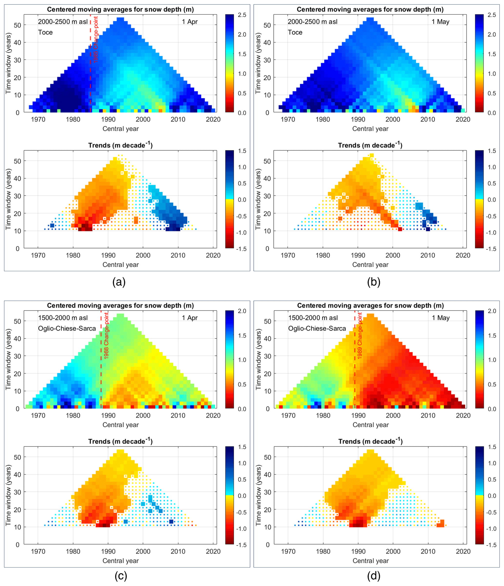
Figure 2Moving Average and Running Trend Analysis (MARTA triangles) of snow depth on 1 April (a, c) and 1 May (b, d) in the altitudinal class 1500–2000 m a.s.l. for the Toce and 2000–2500 m a.s.l. for the Oglio-Chiese-Sarca macro-basins. In the top part of each panel, the statistically significant change point detected by Pettitt's test (5 % significance) is reported as a dashed line, while in the bottom part the statistically significant trends with 5 % significance level of the Mann–Kendall test are reported as thicker pixels.
Table 2Trends of snow depth (1967–2020) for each macro-basin, elevation class (EC) and date. Only statistically significant results according to Mann–Kendall and Student's t tests are reported. If only one test is passed, then the trend is marked with an asterisk; cases in which there are not enough data are flagged as ND (no data). If the trend is not statistically significant for either of the two tests, the value is not reported (–).
Subsequently, we evaluated the difference in average snow depth for each macro-basin, elevation class and date of measurement. Figure 3 shows the average snow depth computed over the monitoring periods 1967–1993 (red circles) and 1994–2020 (black circles). If the difference between the averages of the two samples is statistically significant according to the Mann–Whitney U test, the circles are filled. To improve readability of the plot, an upward or downward blue arrow is reported if an increasing or a decreasing statistically significant trend is present (Table 2), respectively. In the case of the Toce basin, at the lower altitudes, a statistically significant difference has been found only in April, together with a statistically significant decreasing trend, with an average decrease of 0.32 m. However, in the elevation class 1500–2000 the difference in snow depth in the two periods is statistically significant from 1 March to 1 June, with a decrease of 0.37 m; in the elevation class 2000–2500 the average difference between the two periods is 0.38 m, statistically significant from 1 April. The Serio-Brembo and Oglio-Chiese-Sarca macro-basins exhibit the strongest differences between the two periods, statistically significant for 90 % of the cases. At the two lowest altitudes, the difference between the two periods is similar, with an average decrease of 0.28 m (1000–1500) and 0.39 m (1500–2000) for Oglio-Chiese-Sarca and of 0.26 m (1000–1500) and 0.41 m (1500–2000) for Serio-Brembo. In the elevation class 2000–2500, the difference between the two periods in the Serio-Brembo macro-basin (0.78 m) is more than twice larger than the one obtained for Oglio-Chiese-Sarca (0.33 m). Measurements of snow depth in the elevation class 2500–3000 show a statistically significant difference of 0.54 m on average starting from 1 April in the Oglio-Chiese-Sarca macro-basin. We found a similar behavior in the Adda basin for the elevation classes 1500–2000 and 2000–2500, with a statistically significant difference of 0.39 and 0.40 m, respectively. The Adige basin exhibits fewer statistically significant differences, mainly in the two central elevation classes, with an average decrease of 0.21 m (1500–2000) and 0.19 m (2000–2500). In the Piave-Brenta basin, the difference in snow depth between the two periods is statistically significant in 89 % of the cases at the three lowest elevation classes, with decreases of 0.21 m (1000–1500) and 0.29 m (1500–2000 and 2000–2500). These results are coherent with the decrease computed by Lejeune et al. (2019) for a mid-altitude (1325 m a.s.l.) mountain site in France (Col de Porte). They estimated a decrease of 0.39 m in snow depth between the 1969–1990 and 1991–2017 periods. The results obtained show different trends for the considered regions. In view of this, Matiu et al. (2021) pointed out the difficulties in generalizing the results to the whole Alpine area, thus supporting the value of our in-depth analysis in different macro-basins.
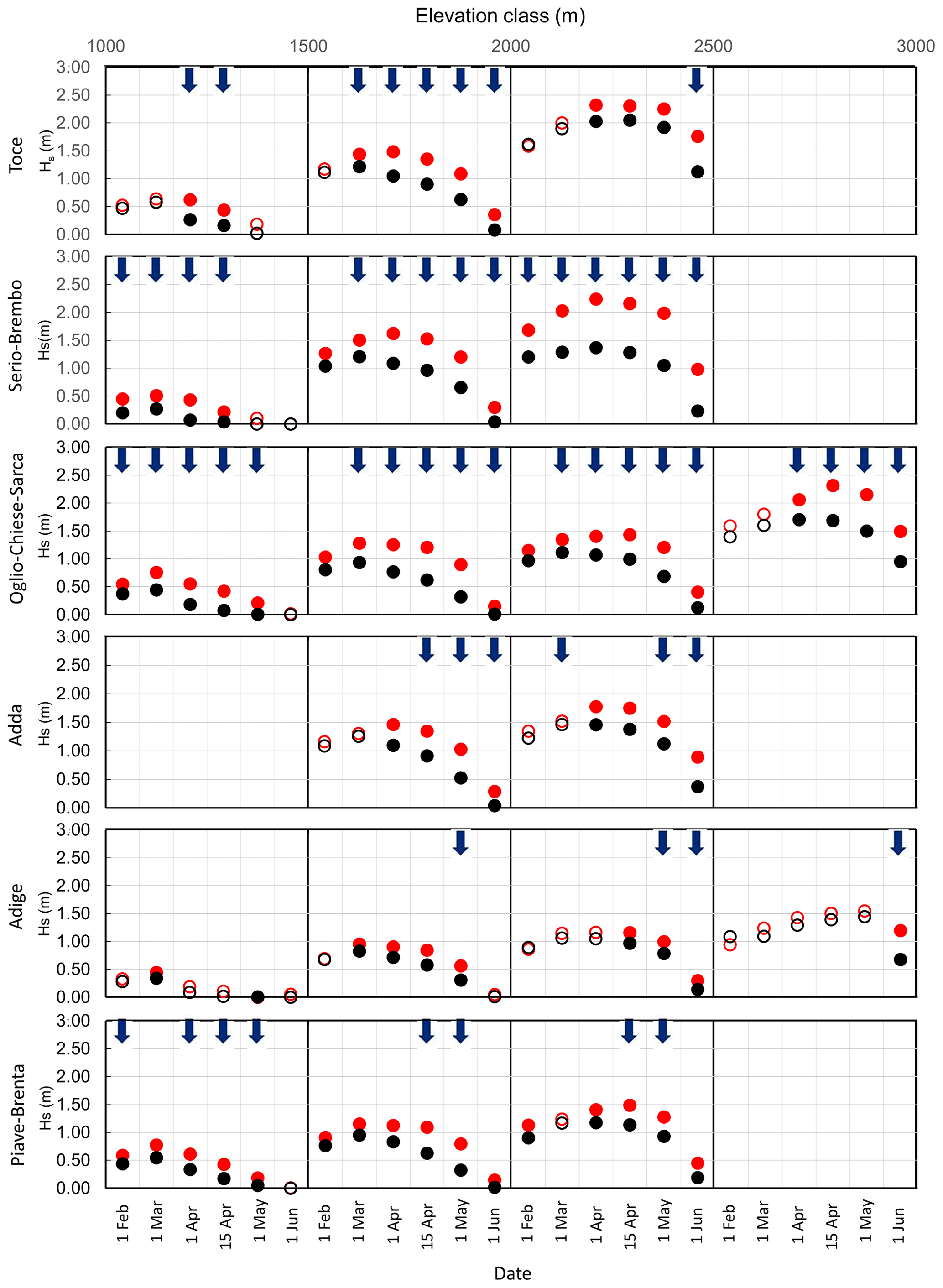
Figure 3Average snow depths (Hs) in the 1967–1993 (red circles) and 1994–2020 (black circles) periods are plotted for each elevation class in the six observation campaign dates (1 February, 1 March, 1 April, 15 April, 1 May, 1 June). Statistically significant (p ≤ 0.01, Mann–Kendall test) trends of the entire 1967–2020 period are sketched as upward (downward) blue arrows for increasing (decreasing) trends. Circles are filled if the difference of Hs between the two periods is statistically significant (p ≤ 0.01, Mann–Whitney U test).
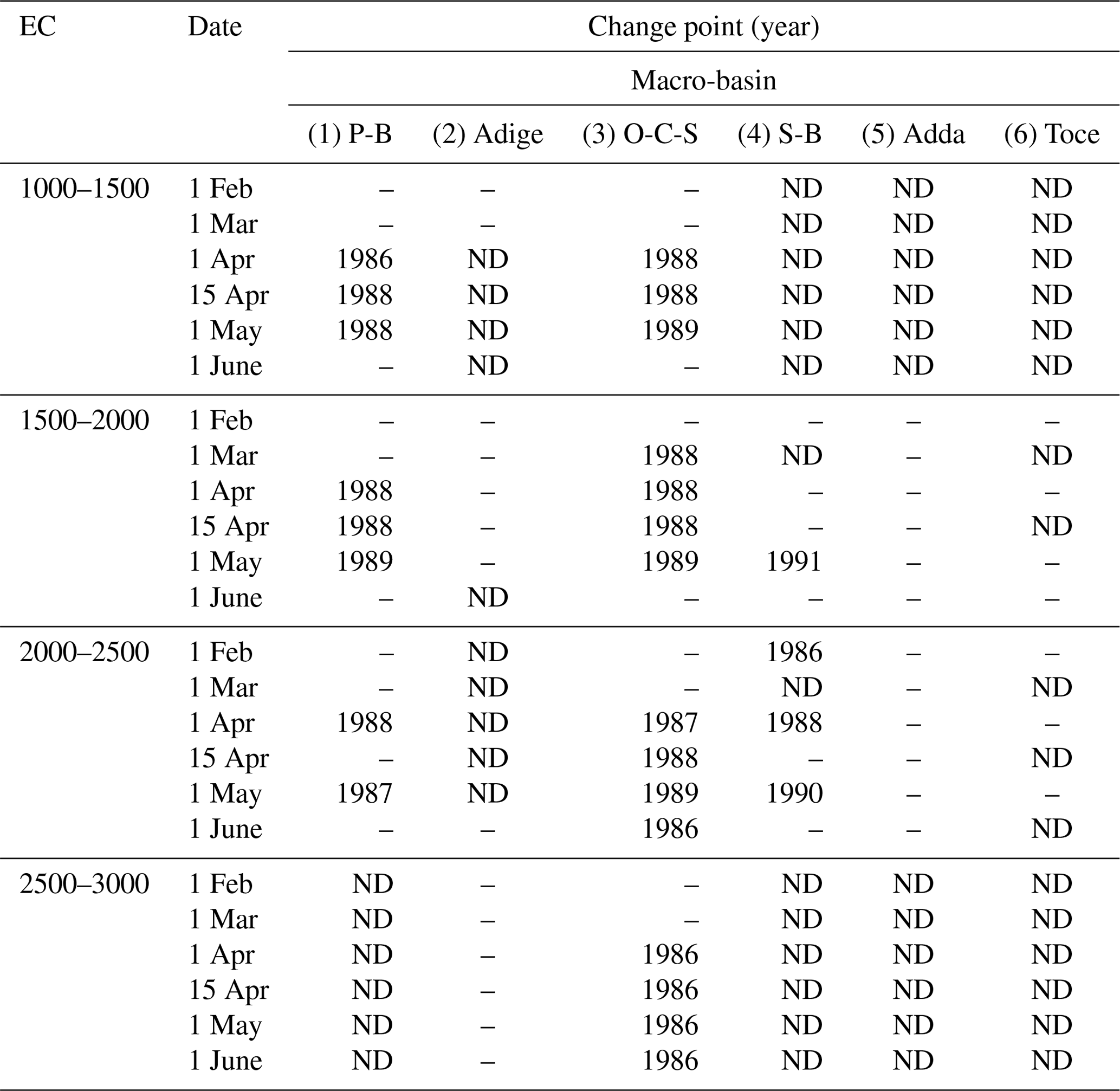
Table 3Years of change points detected by Pettitt's test in snow depth time series for each macro-basin, elevation class (EC) and date. Only statistically significant results are reported, while cases in which there is not enough data are flagged as ND (no data). If the change point is not statistically significant for either of the two tests, the value is not reported (–).
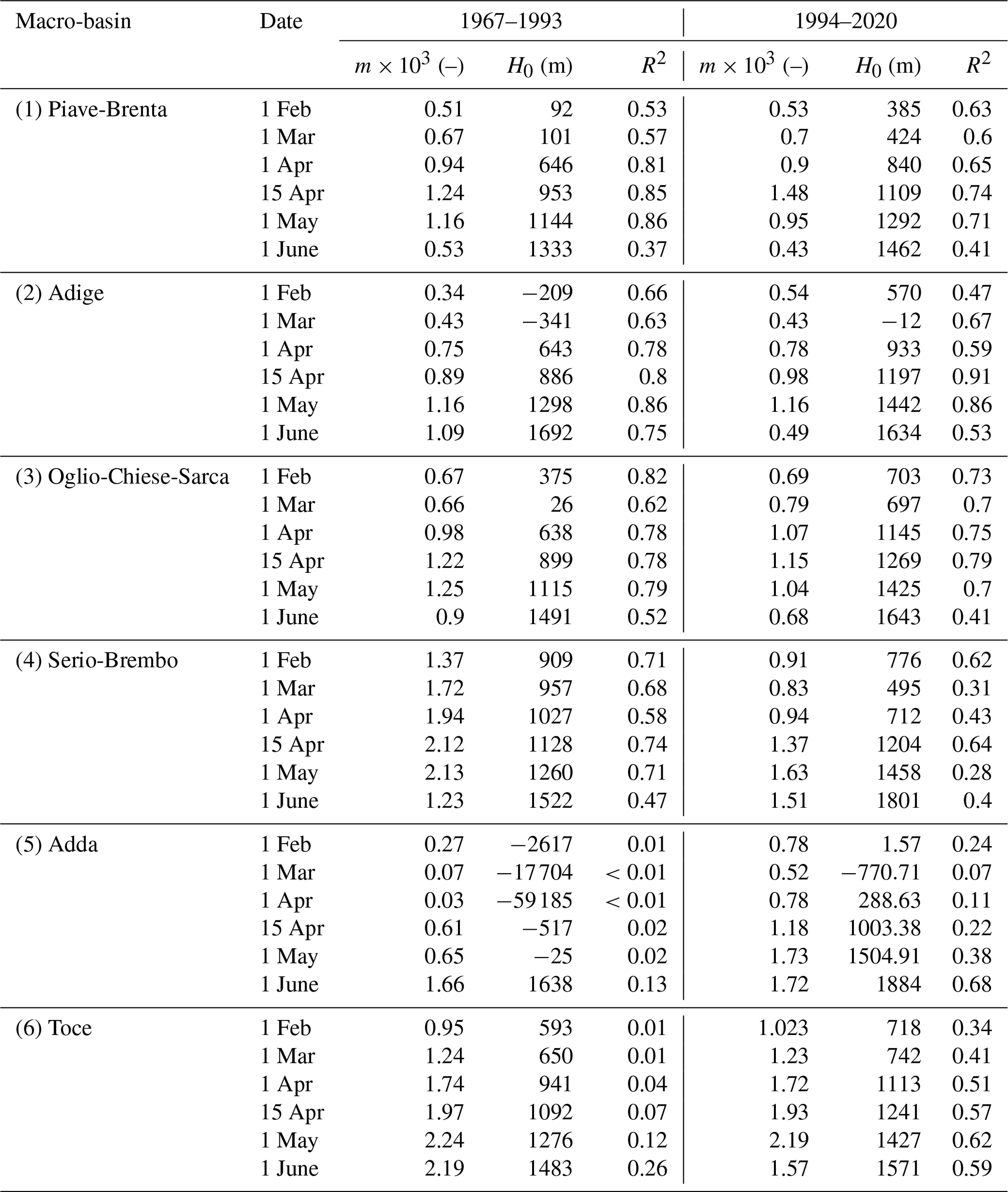
Finally, we evaluated the elevation dependency of snow depth in each area for each measurement date. In Table 4 we report the values of m and H0 least-square regression coefficients fitting average snow depth vs. altitude in Eq. (3). Since the results of the Mann–Whitney U test suggest that there is, in general, a statistically significant difference between the first and second halves of the observation period, we present the results for both the 1967–1993 and 1994–2020 sub-periods. Together with the coefficients obtained from the linear regression analysis, we report the R2 values for each case as an indicator of goodness of the fitting function. The Oglio-Chiese-Sarca, Serio-Brembo and Piave-Brenta macro-basins show higher values of R2 and a common behavior of m and H0. In these basins, m increases after February (accumulation), showing a peak value in spring, reinforced by the earlier onset of the melting season at lower elevations, and then decreases as melting develops at higher elevations. In fact, during the accumulation period the principal factor affecting m is the change from rain to snow with elevation, while during the melt period it is more affected by the variation in melt with elevation (USACE, 1956). On the other hand, H0 exhibits an almost stable or decreasing behavior during the accumulation phase, strongly increasing as the melting season starts. We also observe that H0 exhibits higher values in the second half of the monitoring period, indicating that the elevation of null snow depth has moved towards higher altitudes, according to the hypothesis of decreasing snow depth. Such results confirm the tendency that was modeled by Giorgi et al. (1997), who studied the elevation dependency of surface climate change impacting snow depth over the Alpine region. The results obtained for Adige show similar results, although presenting lower values of R2 (between 0.63 and 0.85), while the model is not reliable for the Toce and Adda basins (R2 ranging from 0 to 0.26). The differences found in this regression analysis are affected by the different spreads of the data between elevation classes described in Sect. 2.2, with the Oglio-Chiese-Sarca, Piave-Brenta and Serio-Brembo basins better covered from the lowest elevation class (1000–1500).
Table 4Linear regression coefficients (m and H0) and R2 of the least-square linear fitting of average snow depth and elevation for the two sub-periods 1967–1993 and 1994–2020.
3.2 Snow density
In order to investigate possible variability and tendencies of snow depth and SWE, we evaluated also bulk snow density data variations with elevation and time. In Fig. 4a we show as an example the bulk snow density plotted as a function of the elevation for the six considered measurement dates in all the considered macro-basins. We found that, within each elevation class, bulk snow density does not substantially vary with elevation for a specific measurement date. On the other hand, we found that bulk snow density increases with measuring date, in accordance with the results found by many authors (Strum et al., 2010; Pistocchi, 2016; Guyennon et al., 2019). Such behavior is common among all the macro-basins studied. In Fig. 4b we report the average bulk snow density computed over the monitoring period. From a least-square fitting of Eq. (2), we obtained new values for the polynomial coefficients, better modeling the data here-presented (R2=0.998) and compared with the model from Guyennon et al. (2019). Specifically, we obtained n0=277, and n2=0.0051, which are more representative for our dataset and more suitable to be used in the considered basins. Such a seasonal increase in snow density is related to different processes such as compaction and increase in liquid water in the snowpack due to melting as the temperature increases.
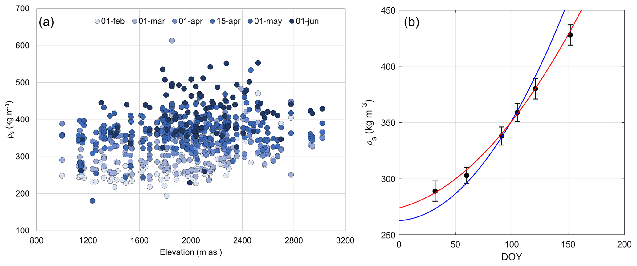
Figure 4(a) Bulk snow density dependence on elevation. Average bulk snow density for each measurement date is represented with different color intensity with changing date of the year. (b) Temporal variability of bulk snow density. Average bulk snow density for each measurement date is represented as a black diamond, and the error bars represent the standard deviation. We also report in red the computed polynomial model and in blue the one proposed in Guyennon et al. (2019).
3.3 Snow water equivalent
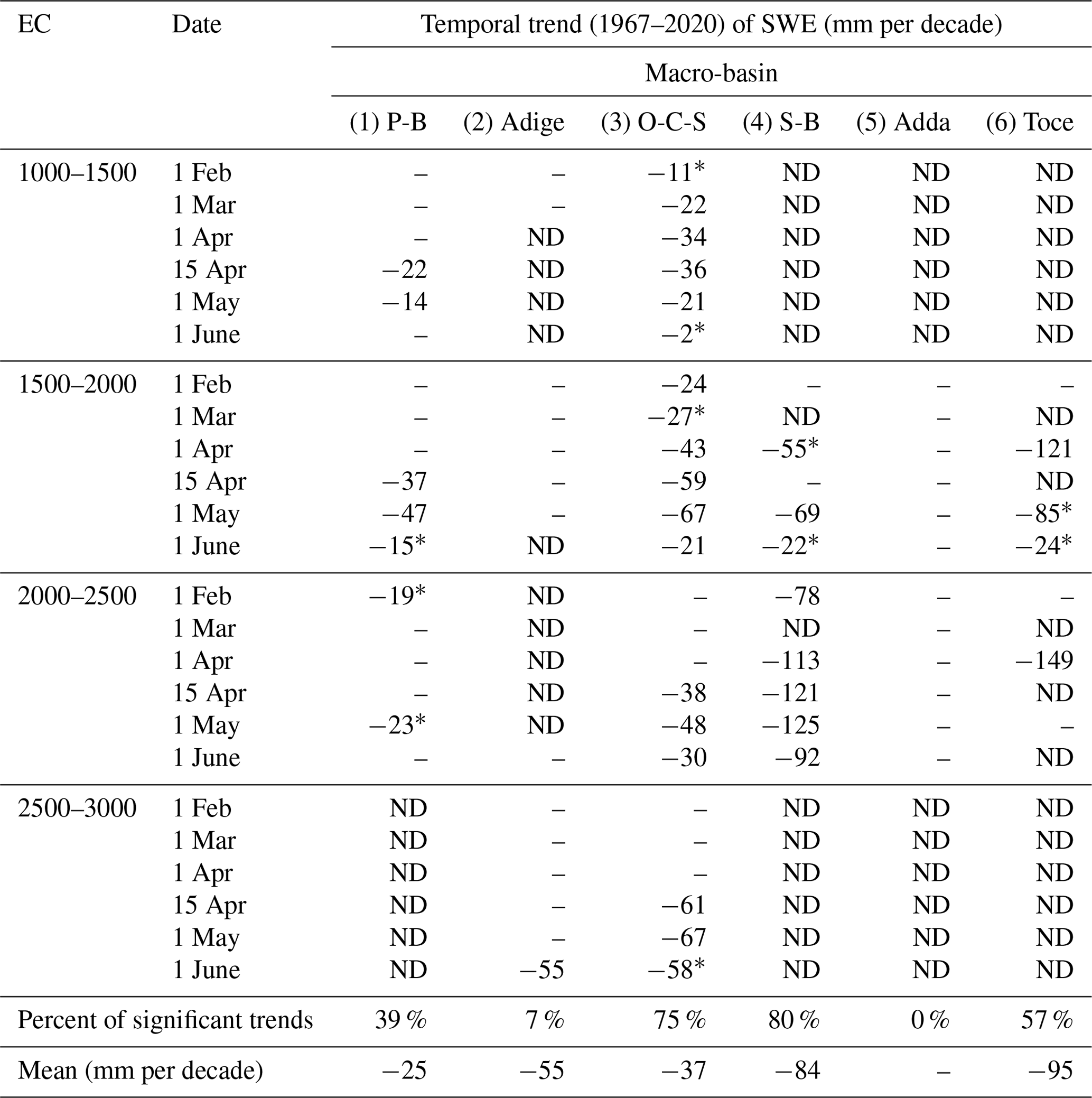
For the available SWE measurements, we computed the temporal trends for each macro-basin, elevation class and date of measurement. In Table 5 we report the temporal trends computed over the monitoring period 1967–2020. The general behavior is in accordance with the one found in the case of snow depth, showing a decreasing trend. Among the considered time series with sufficient SWE measurements, we obtained statistically significant trends in 44 % of the cases according to the MK or Student's t test. The significant trends for all the elevation classes and measurement dates are all negative and on average −51 mm per decade with a standard deviation of 37 mm per decade. Assuming that the slope of the non-significant trends is zero, the average becomes −23 mm per decade with a standard deviation of 35 mm per decade. As for the snow depth, also the absolute value of the SWE trends increases from the eastern to the western macro-basins, ranging from −25 mm per decade in the Piave-Brenta basin to −95 mm per decade in the Toce basin. In the Oglio-Chiese-Sarca macro-basin, the computed trends increase in terms of absolute value moving from winter to spring in the two lower elevation classes, reaching a maximum between 15 April (−36 mm every decade for 1000–1500) and 1 May (−67 mm every decade for 1500–2000); in the two higher-elevation classes, we found statistically significant trends for the measurement dates of 15 April, 1 May and 1 June, suggesting that the spring snow has been more strongly affected in the past decades, reaching a maximum absolute value in May (−48 mm every decade for 2000–2500 and −67 mm every decade for 2500–3000). In Table 6 we report the results of the change-point analysis performed by means of Pettitt's test. The change points obtained range from 1986 to 1991, with 1988 being both mode and median. Specifically, the most frequent change-point years are 1989 (f=17 %), 1986 (f=27 %) and 1988 (f=46 %). The Pettitt test confirms on a sound statistical basis the findings of other studies, such as Marty et al. (2017), based on SWE measurements, and Colombo et al. (2022), based on snow depth measurements and SWE modeling. Valt and Cianfarra (2010) obtained similar results, finding breakpoints between 1984 and 1994. Also in this case, the Oglio-Chiese-Sarca macro-basin exhibits statistically significant results for the largest cases of elevation classes and measurement dates. For this specific macro-basin, we found the significant change points mainly in April and May, in agreement with the results obtained for the long-term trends.
Table 5Trends of snow water equivalent (SWE, 1967–2019) for each macro-basin, elevation class (EC) and date. Only statistically significant results according to Mann–Kendall and Student's t tests are reported. If only one test is passed, the trend is marked with an asterisk, while cases in which there are not enough data are flagged as ND (no data). If the trend is not statistically significant for either of the two tests, the value is not reported (–).
As for the case of snow depth, we evaluated the difference in average SWE for each macro-basin, elevation class and date of measurement. In Fig. 5 we report the average SWE computed over the monitoring periods 1967–1993 (red circles) and 1994–2020 (black circles). The Oglio-Chiese-Sarca macro-basin presents statistically significant results in most cases. We found that the largest statistically significant differences in SWE between the two periods is in spring, for the measurement dates of 1 April and 15 April for the 1000–1500 elevation class and 15 April and 1 May for the other cases. The average difference between the two periods is 85 mm for the elevation class 1000–1500, 135 mm for 1500–2000, 104 mm for 2000–2500 and 226 mm for 2500–3000. The Piave-Brenta macro-basin shows similar results, with statistically significant differences in 89 % of the cases. We found the largest statistically significant differences on 1 April and 15 April for the 1000–1500 elevation class, with an average difference of 59 mm; on 15 April and 1 May for the 1500–2000 elevation class, with an average difference of 82 mm; and on 1 May and 1 June for the 2000–2500 elevation class, with an average difference of 78 mm. For the Adige basin, we found significant differences mainly in the 1500–2000 elevation class, with an average difference of 70 mm. For the Toce and Serio-Brembo macro-basins, the estimate of SWE appears less robust than in the other basins, mainly because of the fewer available measurements of bulk snow density, resulting in more scattered time series in Fig. 5. The Adda basin exhibits significant differences in the 1500–2000 and 2000–2500 elevation classes, with average differences of 141 mm and 104 mm, respectively. Similarly, Marty et al. (2017) observed a stronger decrease in SWE at higher altitudes. Moreover, they also found larger decreases for April SWE than for February SWE, in agreement with our results.
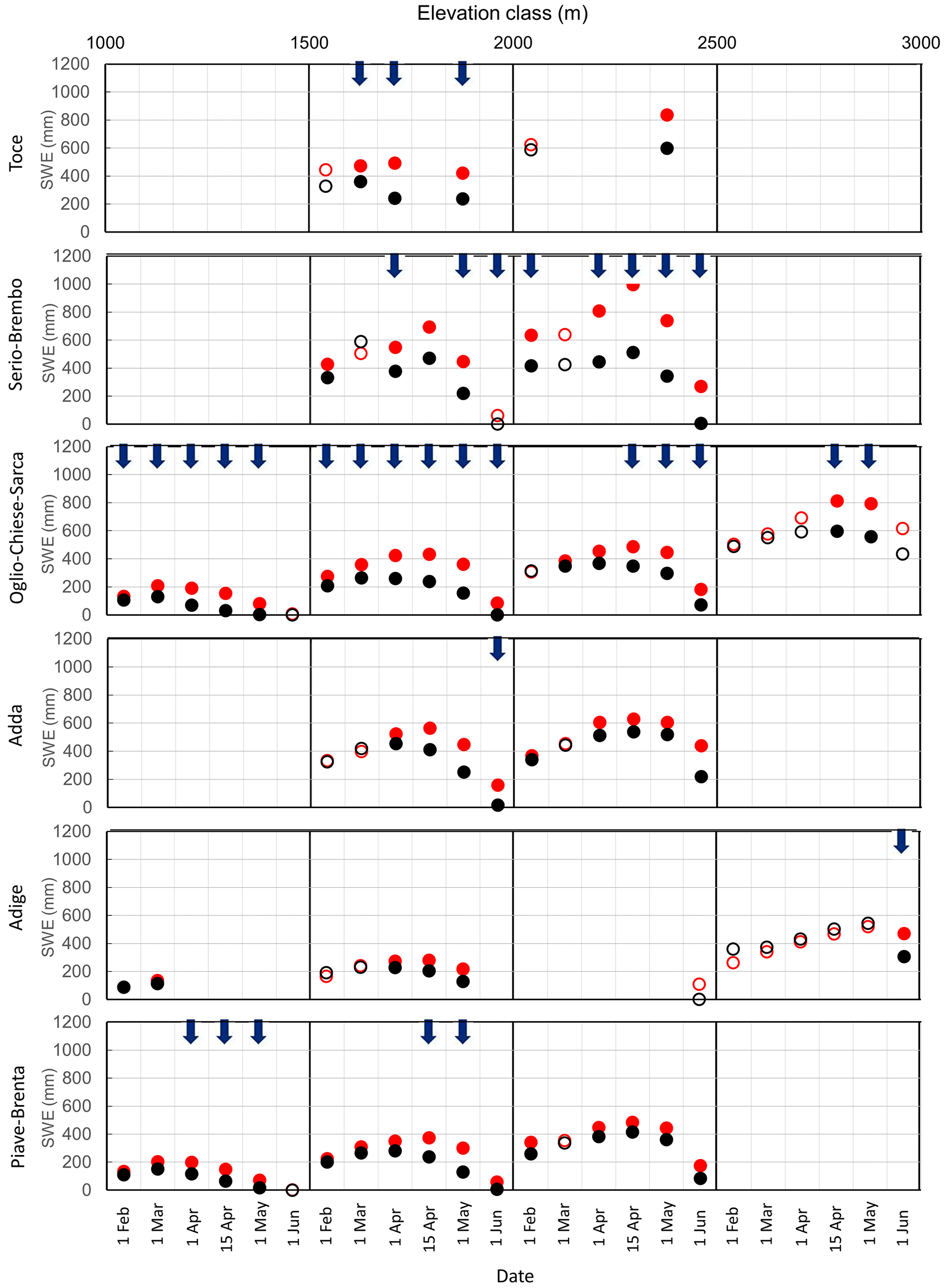
Figure 5Average snow water equivalent (SWE) in the 1967–1993 (red circles) and in 1994–2020 (black circles) periods are plotted for each elevation class in the six observation campaign dates (1 February, 1 March, 1 April, 15 April, 1 May, 1 June). Statistically significant (p ≤ 0.01, Mann–Kendall test) trends of the entire 1967–2020 period are sketched as upward (downward) blue arrows for increasing (decreasing) trends. Circles are filled if the difference of SWE between the two periods is statistically significant (p ≤ 0.01, Mann–Whitney test).
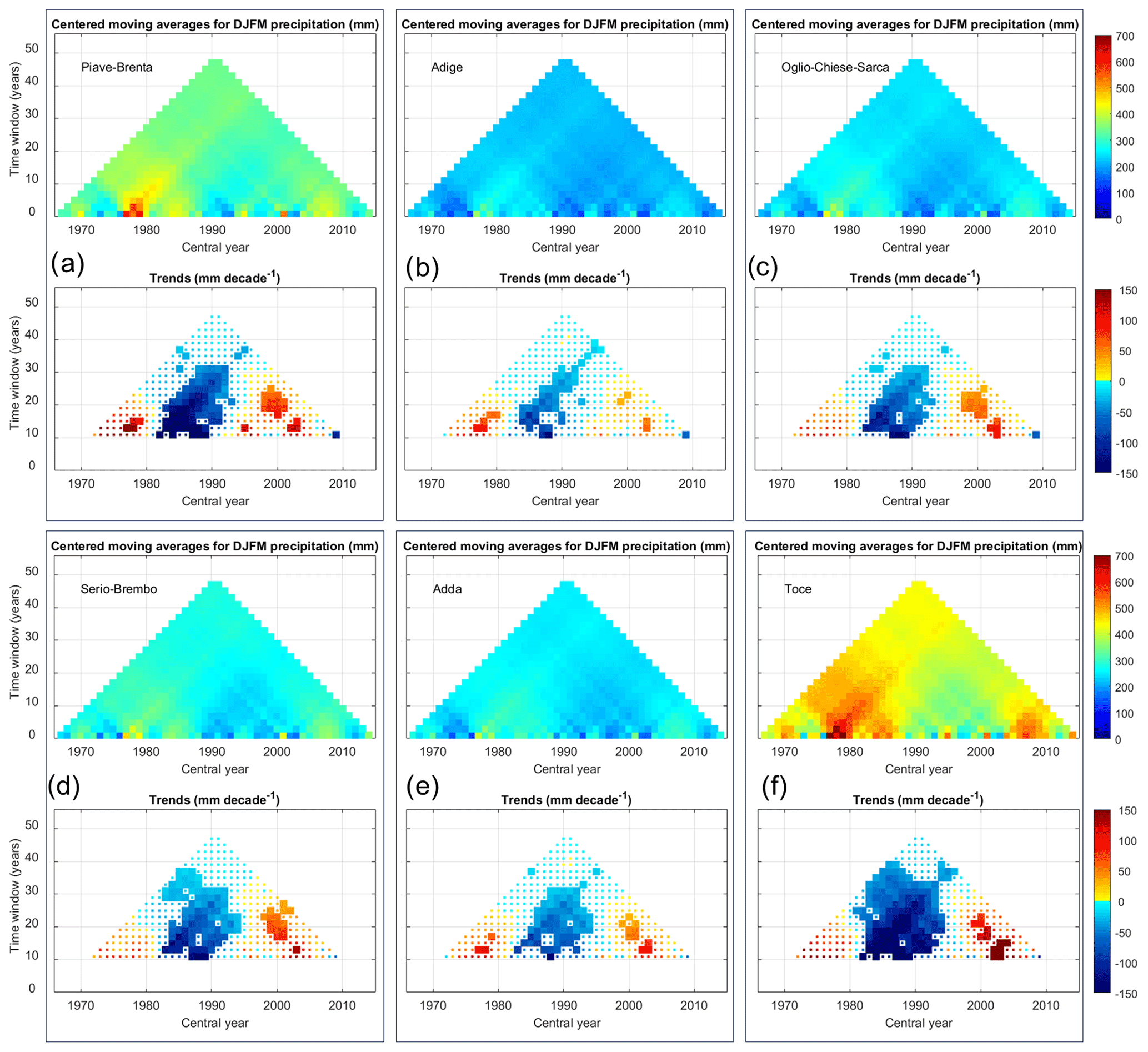
Figure 6MARTA triangles of total winter (DJFM) precipitation for the six macro-basins (in panel a Piave-Brenta, b Adige, c Oglio-Chiese-Sarca, d Serio-Brembo, e Adda and f Toce) from the HISTALP dataset. In the bottom part the statistically significant trends with 5 % significance level of the Mann–Kendall test are reported as thicker pixels.
3.4 Climate variability
In order to evaluate possible links between climate variability and changes that occurred during the monitoring period and the amount and persistence of snow in the considered macro-basins, we also performed MARTA on temperature and precipitation data. Specifically, we considered the average DJFM precipitation and temperature obtained for each macro-basin from the HISTALP dataset. We report the results of the precipitation analysis in Fig. 6 and the temperature analysis in Fig. 7. For all the considered macro-basins, DJFM precipitation exhibits a slight non-significant decrease over the monitoring period, and no statistically significant change point is detected according to Pettitt's test (Fig. 8). By looking at the sub-periods between 10 and 20 years, it is possible to notice three areas of statistically significant trends, showing an increase before 1980, a decrease around 1990 and another increase around 2000, confirming a non-uniform tendency over the complete monitoring period. By comparing the precipitation and snow depth MARTA triangles (Fig. 2), it is possible to notice the similar pattern of wet and dry fluctuations in the moving-average chart. The wet years in terms of precipitation before 1980 and 2010, clearly visible, for example, in the Toce basin in Fig. 6f (slightly weaker signal in the Piave-Brenta basin and weaker yet visible in the other four basins), can be also found in the snow depth moving-average chart, with a stronger pulse before 1980, possibly related to the lower average temperature recorded in those years with respect to the years before 2010 (Fig. 7f). We also performed the same statistical analysis to the HISTALP mean monthly temperature averaged over all the basins (not shown here), to evaluate possible differences in climate variability between accumulation and melting seasons. Temperature increases significantly in both the accumulation (from January to March) and, even more significantly, the melting period (April and May), consistently with results reported by many authors such as Auer et al. (2007) and Brunetti et al. (2009). These results explain the decrease in snow depth and SWE on 1 April and the accelerated melt in the 15 April–1 June period. Both winter (DJFM) and spring (April and May) temperatures exhibit a marked increase after 1987, where a change point is detected by Pettitt's test. This result is consistent with the change point detected in the snow depth and SWE time series, suggesting a strong impact of temperature increase, especially in spring, on snowmelt. The combined effect of precipitation and temperature variability is consistent with the observed stationarity of winter (February and March) snow depth and SWE, the significant decrease in the maximum SWE observed in April and the accelerated melt in May. Marty et al. (2017) found similar result, linking the strong low-elevation SWE decreases to temperature increases and decreasing snow / rain ratio. Colombo et al. (2023) studied the relation between March SWE and winter precipitation and temperature anomalies, obtaining results in agreement with the ones found by Marty et al. (2017). The combination of low-temperature and precipitation anomalies, enhancing dry and warm conditions in the December to March period, is correlated with strong negative anomalies in March SWE, such as the ones that occurred in 2022 (Colombo et al., 2023). Our results confirm those obtained by Marty et al. (2017), showing that winter (DJFM) temperature and precipitation regulate April SWE. These results confirm the impact of temperature rise on snow, affecting consequently the hydrological cycle and water availability.
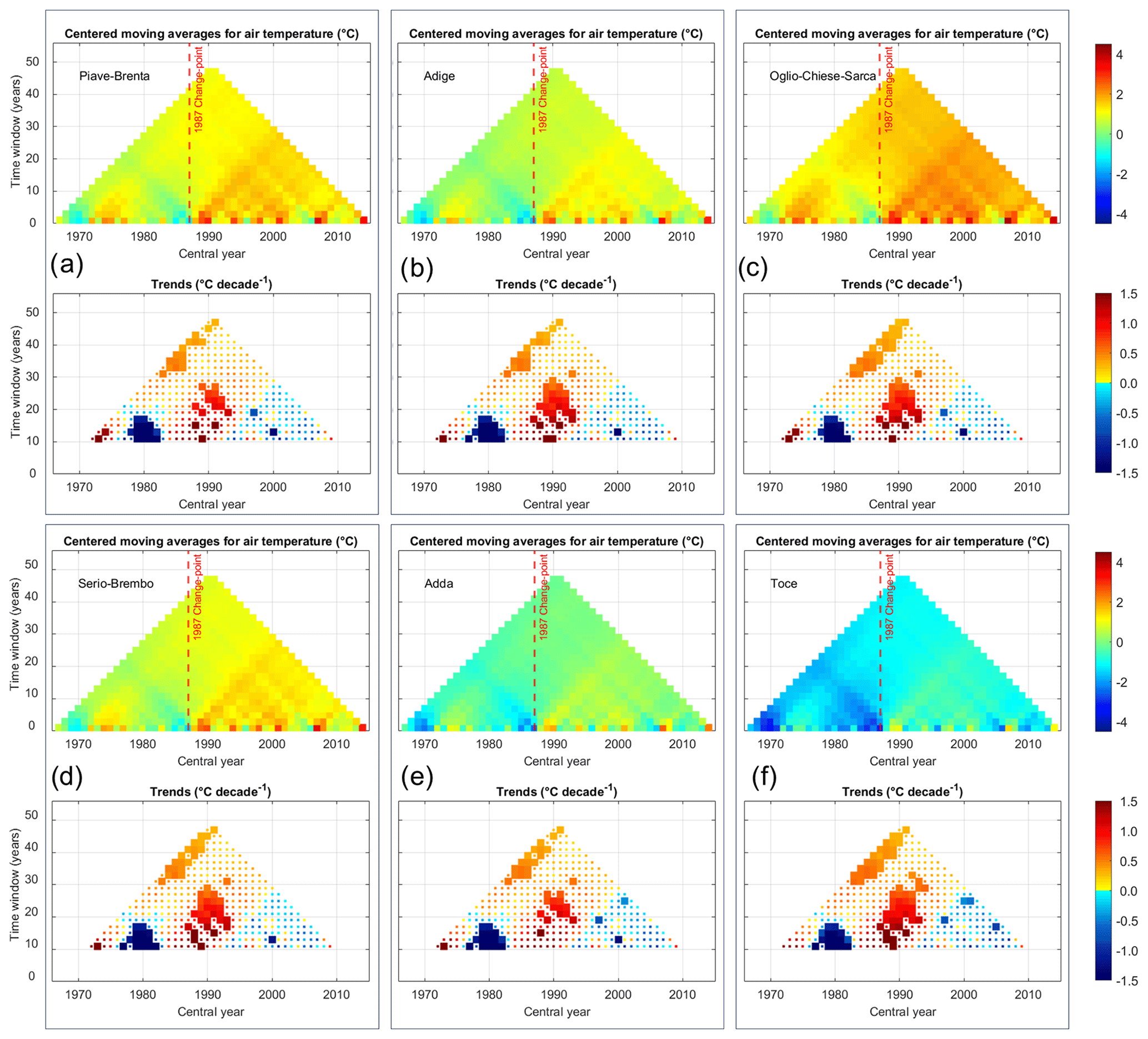
Figure 7MARTA triangles of average winter (DJFM) temperature for the six macro-basins (in panel a Piave-Brenta, b Adige, c Oglio-Chiese-Sarca, d Serio-Brembo, e Adda and f Toce) from the HISTALP dataset. In the top part of each panel the statistically significant change point detected by Pettitt's test is reported as dashed line while in the bottom part, the statistically significant trends with 5 % significance level of the Mann–Kendall test are reported as thicker pixels.
Table 6Years of change points detected by Pettitt's test in SWE time series for each macro-basin, elevation class (EC) and date. Only statistically significant results are reported, while cases in which there are not enough data are flagged as ND (no data). If the change point is not statistically significant for either of the two tests, the value is not reported (–).
Finally, we evaluated the correlation between snow depth on 1 and 15 April and the DJFM NAO and WeMO indexes. In Table 7 we report the statistically significant Pearson's correlations, where the columns represent the six macro-basins and the rows the four elevation classes. We obtain a negative statistically significant Pearson's correlation between winter NAO and spring snow depth, ranging between −0.30 and −0.55 for 1 April and between −0.29 and −0.49 for 15 April. These results are coherent with previous studies of several authors as Steirou et al. (2017), who found linkages between NAO and precipitation in Europe; Colombo et al. (2022) found a negative correlation between NAO and SWE indexes, while Bertoldi et al. (2023) found a negative correlation between NAO and snow depth. The WeMO index exhibits an opposite link with snow depth, with positive statistically significant correlations ranging between 0.27 and 0.37 for 1 April and between 0.27 and 0.40 for 15 April, in agreement with the positive correlation between winter WeMO and precipitation (0.38) obtained by Ranzi et al. (2021). Considering the role of NAO and WeMO in winter precipitation, proved in the mentioned literature, the correlations we found between these two indexes and April snow depth for the complete time period enforce the results concerning the role of precipitation in regulating the interannual variability of snow depth. Periods of high NAO values are characterized by lower winter precipitation and, consequently, lower snow depth in April. On the other hand, periods of high WeMO are correlated with dryer conditions and with low-snow-depth measurements. These results imply a relation between atmospheric circulation patterns and interannual variability of snow depth. Preliminary analysis of wavelet coherence spectra (not reported here) for the Oglio-Chiese-Sarca basin confirm a significant coherence for a period localized in the proximity of the wet pulse observable in both snow depth and precipitation MARTA triangles around 1980. Similarly, we observed a coherence spot around 2010, statistically significant only for the 1500–2000 elevation class and visible but not statistically significant for the 2000–2500 elevation class, less extended than the one temporally located in 1980. For both late 1980s and 2010 local coherence areas, Bertoldi et al. (2023) found negative changing points of snow depth during a positive NAO phase for the former and at the very end of a negative NAO phase for the latter, accompanied by a temporary decrease in temperature.
Table 7Statistically significant (p < 0.05) Pearson's correlation between winter average teleconnection indexes NAO and WeMO and snow depth measured on 1 April and 15 April for the considered basins and for the four considered elevation classes.
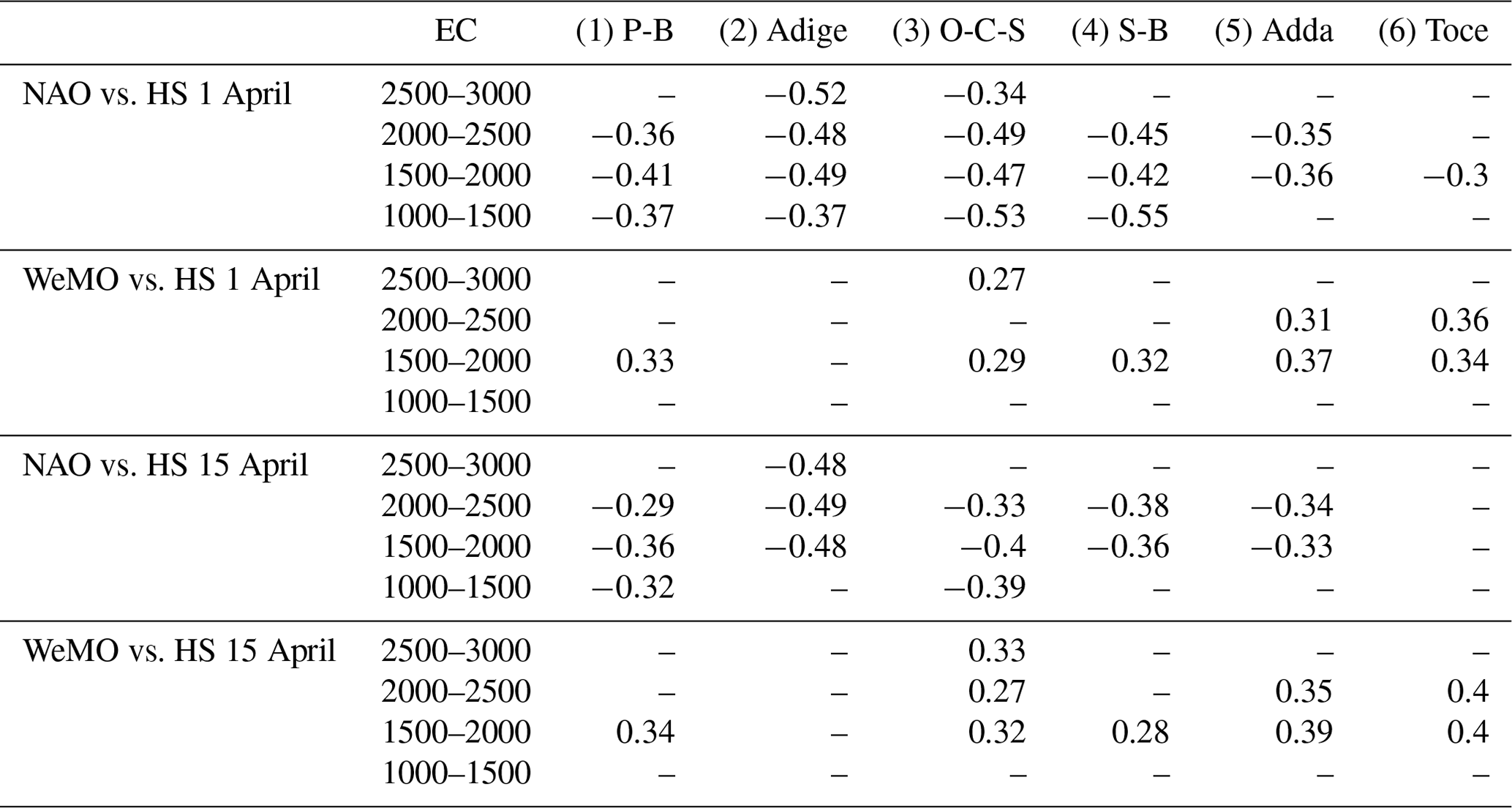
Table 8Parameters of the climatological third-order polynomial snow depth model for the sub-periods 1967–1993 and 1994–2020.

3.5 Mean snow climatology model
Here we show the results obtained from the SWE regression model presented in Sect. 2.6, applied to the case of the Oglio-Chiese-Sarca macro-basin. In Fig. 8 we show the values of m (Fig. 8a) and H0 (Fig. 8b) obtained from the linear regression analysis of average snow depth measurements for the monitoring periods 1967–1993 (gray triangles) and 1994–2020 (black diamonds) obtained from Table 4. We selected the Oglio-Chiese-Sarca macro-basin as it shows the highest R2 values (Table 3) and the second half of the monitoring period as more representative of the current nivological situation. The best fits of Eqs. (4) and (5) are plotted as dotted black lines. The coefficients a0, a1, a2, a3, b0, b1, b2 and b3 are reported in Table 8. The fitting curves well describe the observed behavior presented in Sect. 2.1, showing high values of R2 (0.99 for both m and in the first period and H0 0.97 for m and 0.99 for H0 in the second period). Such a fitting must be considered valid only within the considered time period, as it might introduce strong uncertainty due to the low number of points adopted for the fitting procedure. However, the curve obtained provides an analytical function to estimate the temporal evolution of the linear regression coefficients m and H0.
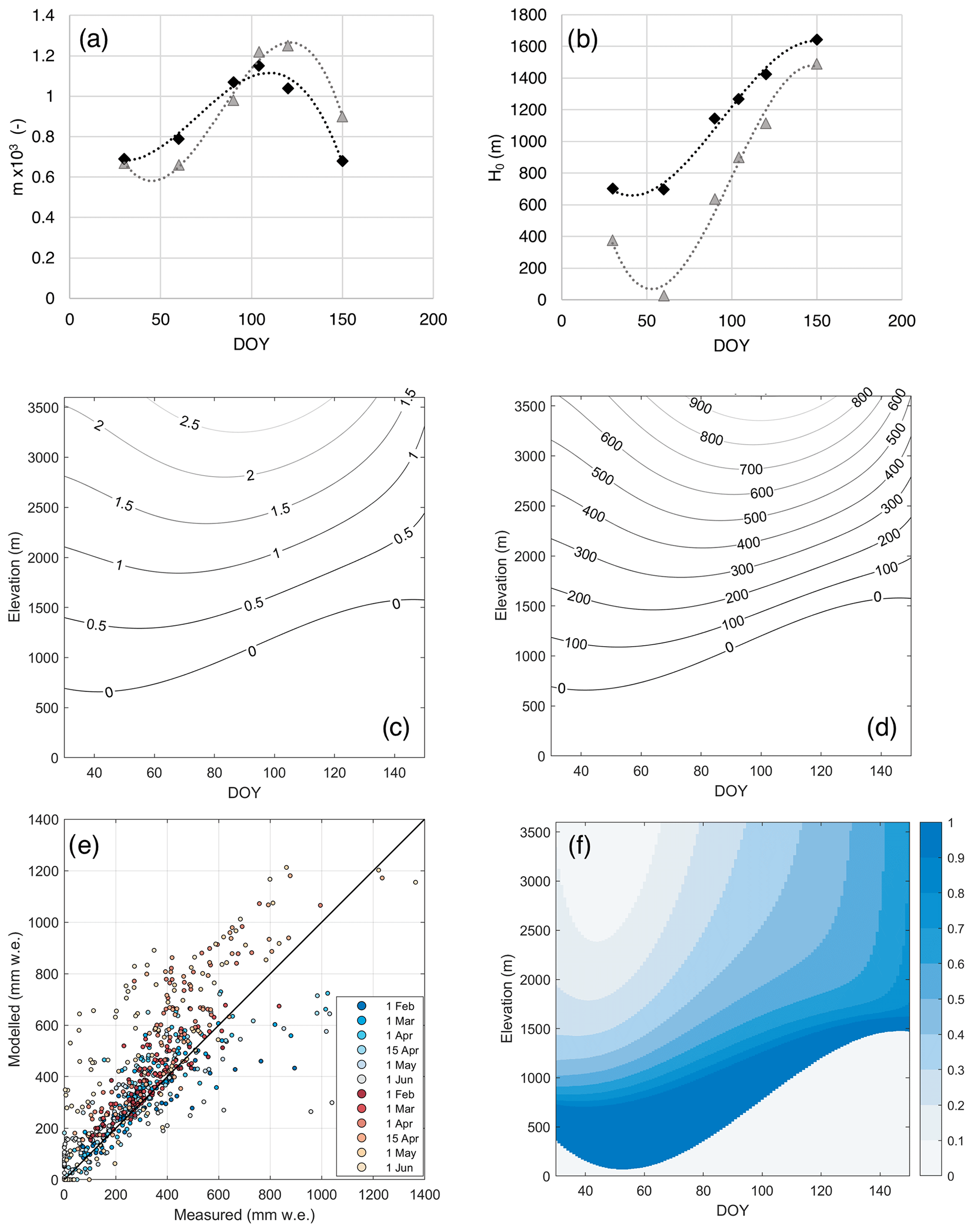
Figure 8Slope m (a) and null snow depth elevation H0 (b) as a function of the day of the year for the sub-periods 1967–1993 (gray triangles) and 1994–2020 (black diamonds). Dotted lines represent the third-order polynomial fitting curve (Eqs. 4 and 5). Contour plots of snow depth (c) and snow water equivalent (d) in the time–elevation (DOY–H) space for the 1994–2020 sub-period. In panel (e) the scatterplot reports measured and modeled climatological SWE in the Oglio-Chiese-Sarca macro-basin for the first (red) and second (blue) sub-periods. Panel (f) reports the comparison between the modeled climatological SWE in the first and in the second sub-periods, expressed as relative decrease in SWE (unitless).
The coefficients n0, n1 and n2, to define the second-order polynomial function of ρs, are reported in Sect. 3.2. With the estimates of m, H0 and ρs obtained from the long-term snow depth and bulk snow density observations, it is possible to estimate the SWE in the DOY–H space as shown in Fig. 8c and d. From the contour plot, we observe that the DOY of maximum SWE for fixed elevation (DOY of the local minimum of the SWE isolines) linearly shifts in time, confirming the behavior observed in the previous sections. However, for elevations higher than 2500 m a.s.l., we consider the model less reliable as the number of snow depth measurements is lower at such elevation, and above a certain point snow depth might reach a plateau or even decrease (Grünewald et al., 2014). We evaluated the uncertainty in the estimate of the expected value of SWE at given elevation and day of the year obtained by this climatological model by comparing the results of the outputs with the average of SWE measurements at fixed elevation and measurement date (i.e., the average of all the SWE measurements at each single measurement site for each measurement date within the considered sub-period). In Fig. 8e we report the scatterplot of the measured and modeled climatological SWE for the considered sub-periods of observation and measurement dates. We obtained RMSE values of 148 mm of SWE for the first period (R2=0.69) and 97 mm for the second period (R2=0.71). We observe that the maximum error is registered, for both sub-periods, on 1 June, possibly correlated with the low values of R2 of the linear regression model of snow depth. Moreover, the error analysis shows higher errors for higher elevations with the largest differences between model and observations above 2000 m a.s.l. on 1 June (Fig. 8e). This model must be intended in a climatological way, as it has been conceived from average values over a time period of 27 years, and it can provide a simple yet useful estimate of the expected snow water equivalent at a given day of the year and at the specific altitude of interest, albeit constrained by challenges related to knowledge of actual snowpack conditions at elevations exceeding 2500 m and the limited goodness of fit of the snow depth model in June. In Fig. 8f we report the relative difference between the modeled climatological SWE in the two sub-periods, computed as . The representation of the modeled climatological SWE relative difference highlights an almost complete disappearance (decrease >90 %) of SWE below 750 m a.s.l. Above such an elevation, the relative decrease is stronger, moving towards the melting season, with the weakest decrease at high elevations at the beginning of the year, in agreement with the results previously presented.
We studied changes and variability of snow depth and SWE in six macro-basins of the Italian Alps over the monitoring period 1967–2020 based on measurements collected on 1 February, 1 March, 1 April, 15 April, 1 May and 1 June. Our results show the effects of the temperature increase of the past century on snow accumulation in the Italian Alps. We found that all the statistically significant trends are negative in both snow depth (57 % of the cases) and SWE (44 % of the cases) over the years.
All the mean values of snow depth in the first half of the monitoring period (1967–1993) are higher than those in the second one (1994–2020), and for 82 out of the 113 cases (73 %) the two samples are significantly different. The results are the same when considering SWE, with 63 out of the 87 values (72 %) significantly higher in the first half period. Specifically, we found that, as a spatial average throughout all the basins and elevation classes, snow depth decreased by 33 % on 1 April, exhibiting stronger differences between the two periods at lower altitudes (62 % in the 1000–1500 m elevation class) and smaller difference towards higher elevations (30 % at 1500–2000 m, 22 % at 2000–2500 m and 18 % at 2500–3000 m). In the case of SWE, we found a spatial average decrease of 32 % with respect to the 1967–1993 period, higher at low elevations (52 % at 1000–1500 m) and substantially lower at higher altitudes (between 28 % and 29 %). Such results have also been confirmed by the higher values of snowline elevation H0 we obtained for the second period. The computed trends and differences exhibit a strong change in spring (1 April and 15 April mainly) snow depth and SWE, suggesting that spring snowmelt is highly impacted by global warming. Such behavior can have strong effects on the hydrological regime of the considered catchments, possibly modifying magnitude and timing of flood events and affecting water availability in the summer. We found that around 1988, on average, there was a change point, with snow depth and SWE being lower in the following decades. This appears to be a common result for all the macro-basins and elevations. To reject the hypothesis of possible errors in the snow depth and SWE time series due to measurement methodology, variations or other factors affecting the time series reliability, we performed the same change-point detection analysis on measured temperature data from the HISTALP dataset, resulting in a change point in the same period. This result confirms the robustness of our findings and highlights the strong effects of temperature on snow amount and persistency, both in terms of rain–snow separation and melt onset. The analysis of precipitation and temperature data also confirms the weaker variation during the accumulation season (1 February and 1 March) in contrast with the strong decrease in snow depth and SWE during the melting season. The correlation analysis of NAO and WeMO climatological indexes with snow depth on 1 April showed similar correlations obtained in other studies. In fact, we found negative Pearson's correlation coefficient in the case of the NAO index and positive in the case of the WeMO index. Further investigations might highlight the impacts of the observed changes in climatological and nivological conditions on hydropower energy production. The elevation and time dependency analysis of snow depth and bulk snow density measurements allowed for developing a simple SWE model as a function of time and elevation. In fact, as shown in Fig. 4, bulk snow density changes significantly only with the day of the year, being almost constant with altitude. On the other hand, snow depth linearly increases with elevation and, of course, increases along the accumulation season and starts decreasing as the melting season begins. From such an analysis, we obtained the parameters for a simple SWE model that can be applied to estimate the SWE evolution between February and the end of May as a function of the elevation and day of the year. Such a model can be used to estimate SWE for local applications in the considered macro-basins. An error analysis highlighted the limitations of the model performances at high elevations at the end of the season, exhibiting the higher absolute differences with average measured SWE on 1 June.
Future research may involve the utilization of analyzed data for the reconstruction of snow depth and SWE maps, within the targeted basins and possibly over a wider portion of the Alps, employing more sophisticated models, such as advanced machine learning techniques. Additionally, satellite data and remote sensing algorithms may provide valuable support in this context. These methodologies can be further validated, leveraging the insights derived from the present dataset.
The dataset of snow depth and bulk snow density used for this study was provided by Enel. The average values at the macro-basin scale will be made available upon request. The HISTALP dataset is available at https://www.zamg.ac.at/histalp/datasets.php (HISTALP, 2024). The climate oscillation indexes are available at https://www.ncei.noaa.gov/access/monitoring/products/ (NOAA, 2024) and at http://www.ub.edu/gc/wemo/ (last access: June 2021). WeMO and NAO winter (DJFM) averages are reported as a table in the Supplement.
The supplement related to this article is available online at: https://doi.org/10.5194/hess-28-2555-2024-supplement.
RR, PC and GG designed the study and the methodology. PC processed the data and prepared the figures. RR and PC wrote the text. RR, PC and GG edited and reviewed the manuscript.
The contact author has declared that none of the authors has any competing interests.
Publisher's note: Copernicus Publications remains neutral with regard to jurisdictional claims made in the text, published maps, institutional affiliations, or any other geographical representation in this paper. While Copernicus Publications makes every effort to include appropriate place names, the final responsibility lies with the authors.
This article is part of the special issue “Hydrological response to climatic and cryospheric changes in high-mountain regions”. It is not associated with a conference.
Funding for this study has been provided by Cariplo Foundation through the CLIMADA project and by Po River District Basin Authority through grant no. 8536/2020. We gratefully thank the Hydrology and Hydraulic Analysis center of Enel Green Power in Venice-Mestre, specifically Lorenzo Veronese, Francesco Dalla Valle, Ludovica Ruggeri and Alberto Bonafè for the data made available and the collaboration over the last decades. The preliminary results of this research have been presented at the AGU Fall Meeting 2021 (Colosio et al., 2021). We would like to thank Paolo Raccagni and Vladimiro Boselli for their contribution at the earliest stage of the project and Mauro Valt (ARPA Veneto) for his comments.
This paper was edited by Giulia Zuecco and reviewed by Xavier Fettweis and one anonymous referee.
Auer, I., Böhm, R., Jurkovic, A., Lipa, W., Orlik, A., Potzmann, R., Schöner, W., Ungersbock, M., Matulla, C., Briffa, K., Jones, P., Efthymiadis, D., Brunetti, M., Nanni, T., Maugeri, M., Mercalli, L., Mestre, O., Moisselin, J.-M., Begert, M., Müller-Westermeier, G., Kveton, V., Bochnicek, O., Stastny, P., Lapin, M., Szalai, S., Szentimrey, T., Cegnar, T., Dolinar, M., GajicCapka, M., Zaninovic, K., Majstorovic, Z., and Nieplova, E.: HISTALP – historical instrumental climatological surface time series of the Greater Alpine Region, Int. J. Climatol., 27, 17–46, 2007.
Avanzi, F., De Michele, C., and Ghezzi, A.: On the performances of empirical regressions for the estimation of bulk snow density, Geogr. Fis. Din. Quat., 38, 105–112, 2015.
Bavera, D. and De Michele, C.: Snow water equivalent estimation in the Mallero basin using snow gauge data and MODIS images and fieldwork validation, Hydrol. Process., 23, 1961–1972, 2009.
Beniston, M.: Is snow in the Alps receding or disappearing?, WIRes Clim. Change, 3, 349–358, 2012.
Beniston, M., Farinotti, D., Stoffel, M., Andreassen, L. M., Coppola, E., Eckert, N., Fantini, A., Giacona, F., Hauck, C., Huss, M., Huwald, H., Lehning, M., López-Moreno, J.-I., Magnusson, J., Marty, C., Morán-Tejéda, E., Morin, S., Naaim, M., Provenzale, A., Rabatel, A., Six, D., Stötter, J., Strasser, U., Terzago, S., and Vincent, C.: The European mountain cryosphere: a review of its current state, trends, and future challenges, The Cryosphere, 12, 759–794, https://doi.org/10.5194/tc-12-759-2018, 2018.
Berni, A. and Giacanelli, E.: La campagna di rilievi nivometrici effettuata dall'ENEL nel periodo febbraio–giugno 1966, Energia elettrica, 9, 533–542, 1966.
Bertoldi, G., Bozzoli, M., Crespi, A., Matiu, M., Giovannini, L., Zardi, D., and Majone, B.: Diverging snowfall trends across months and elevation in the northeastern Italian Alps, Int. J. Climatol., 43, 2794–2819, 2023.
Blöschl, G.: Scaling issues in snow hydrology, Hydrol. Process., 13, 2149–2175, 1999.
Bocchiola, D. and Diolaiuti, G.: Evidence of climate change within the Adamello Glacier of Italy, Theor. Appl. Climatol., 100, 351–369, 2010.
Brugnara, Y. and Maugeri, M.: Daily precipitation variability in the southern Alps since the late 19th century, Int. J. Climatol., 39, 3492–3504, 2019.
Brunetti, M., Lentini, G., Maugeri, M., Nanni, T., Auer, I., Boehm, R., and Schöener, W.: Climate variability and change in the greater alpine region over the last two centuries based on multi-variable analysis, Int. J. Climatol., 29, 2197–2225, 2009.
Carturan, L., Baroni, C., Brunetti, M., Carton, A., Dalla Fontana, G., Salvatore, M. C., Zanoner, T., and Zuecco, G.: Analysis of the mass balance time series of glaciers in the Italian Alps, The Cryosphere, 10, 695–712, https://doi.org/10.5194/tc-10-695-2016, 2016.
Chimani, B., Böhm, R., Matulla, C., and Ganekind, M.: Development of a longterm dataset of solid/liquid precipitation, Adv. Sci. Res., 6, 39–43, 2011.
Colombo, N., Valt, M., Romano, E., Salerno, F., Godone, D., Cianfarra, P., Freppaz, M., Maugeri, M., and Guyennon, N.: Long-term trend of snow water equivalent in the Italian Alps, J. Hydrol., 614, 128532, https://doi.org/10.1016/j.jhydrol.2022.128532, 2022.
Colombo, N., Guyennon, N., Valt, M., Salerno, F., Godone, D., Cianfarra, P., Freppaz, M., Maugeri, M., Manara, V., Acquaotta, F., Petrangeli, A. B., and Romano, E.: Unprecedented snowdrought conditions in the Italian Alps during the early 2020s, Environ. Res. Lett., 18, 074014, https://doi.org/10.1088/1748-9326/acdb88, 2023.
Colosio, P., Ranzi, R., Boselli, V., Raccagni, P., and Galeati, G.: Climatology of snow depth and snow water equivalent in the Italian Alps (1967–2020), in: AGU Fall Meeting Abstracts, Vol. 2021, AGU Fall Meeting 2021, 13–17 December 2021, New Orleans, LA, C35G-0953, 2021.
Diolaiuti, G., Bocchiola, D., D'Agata, C., and Smiraglia, C.: Evidence of climate change impact upon glaciers' recession within the Italian Alps: the case of Lombardy glaciers, Theor. Appl. Climatol., 109, 429–445, 2012.
Durand, Y., Giraud, G., Laternser, M., Etchevers, P., Mérindol, L., and Lesaffre, B.: Reanalysis of 47 years of climate in the French Alps (1958–2005): climatology and trends for snow cover, J. Appl. Meteorol. Clim., 48, 2487–2512, 2009.
Fierz, C., Armstrong, R. L., Durand, Y., Etchevers, P., Greene, E., McClung, D. M., Nishimura, K., Satyawali, P. K., and Sokratov, S. A.: The International Classification for Seasonal Snow on the Ground, IHP-VII Technical Documents in Hydrology no. 83, IACS Contribution no. 1, UNESCO-IHP, Paris, https://api.semanticscholar.org/CorpusID:130402272 (last access: 11 June 2024), 2009.
Ge, Y. and Gong, G.: North American snow depth and climate teleconnection patterns, J. Climate, 22, 217–233, 2009.
Giorgi, F., Hurrell, J. W., Marinucci, M. R., and Beniston, M.: Elevation dependency of the surface climate change signal: a model study, J. Climate, 10, 288–296, 1997.
Gong, G., Entekhabi, D., Cohen, J., and Robinson, D.: Sensitivity of atmospheric response to modeled snow anomaly characteristics, J. Geophys. Res.-Atmos., 109, D06107, https://doi.org/10.1029/2003JD004160, 2004.
Grünewald, T., Bühler, Y., and Lehning, M.: Elevation dependency of mountain snow depth, The Cryosphere, 8, 2381–2394, https://doi.org/10.5194/tc-8-2381-2014, 2014.
Guyennon, N., Valt, M., Salerno, F., Petrangeli, A. B., and Romano, E.: Estimating the snow water equivalent from snow depth measurements in the Italian Alps, Cold Reg. Sci. Technol., 167, 102859, https://doi.org/10.1016/j.coldregions.2019.102859, 2019.
HISTALP: HISTALP Datasets, https://www.zamg.ac.at/histalp/datasets.php (last access: 12 June 2024), 2024.
IPCC: IPCC Special Report on the Ocean and Cryosphere in a Changing Climate, edited by: Pörtner, H.-O., Roberts, D. C., Masson-Delmotte, V., Zhai, P., Tignor, M., Poloczanska, E., Mintenbeck, K., Alegría, A., Nicolai, M., Okem, A., Petzold, J., Rama, B., and Weyer, N. M., Cambridge University https://doi.org/10.1017/9781009157964, 2019.
Kendall, M. G.: A new measure of rank correlation, Biometrika, 30, 81–93, https://doi.org/10.2307/2332226, 1938.
Kottegoda, N. T. and Rosso, R.: Applied statistics for civil and environmental engineers, Blackwell Publishing, Hoboken, NJ, USA, 2008.
Lehning, M., Grünewald, T., and Schirmer, M.: Mountain snow distribution governed by an altitudinal gradient and terrain roughness, Geophys. Res. Lett., 38, L19504, https://doi.org/10.1029/2011GL048927, 2011.
Lehr, C., Ward, P. J., and Kummu, M.: Impact of large-scale climatic oscillations on snowfall-related climate parameters in the world's major downhill ski areas: a review, Mt. Res. Dev., 32, 431–445, 2012.
Lejeune, Y., Dumont, M., Panel, J.-M., Lafaysse, M., Lapalus, P., Le Gac, E., Lesaffre, B., and Morin, S.: 57 years (1960–2017) of snow and meteorological observations from a mid-altitude mountain site (Col de Porte, France, 1325 m of altitude), Earth Syst. Sci. Data, 11, 71–88, https://doi.org/10.5194/essd-11-71-2019, 2019.
López-Moreno, J. I., Soubeyroux, J. M., Gascoin, S., Alonso-Gonzalez, E., Durán-Gómez, N., Lafaysse, M., M., Vernay, M., Carmagnola, C., and Morin, S.: Long-term trends (1958–2017) in snow cover duration and depth in the Pyrenees, Int. J. Climatol., 40, 6122–6136, 2020.
Mann, H. B.: Nonparametric tests against trend, Econometrica, 13, 245–259, 1945.
Mann, H. B. and Whitney, D. R.: On a test of whether one of two random variables is stochastically larger than the other, Ann. Math. Stat., 18, 50–60, 1947.
Maragno, D., Diolaiuti, G., D'Agata, C., Mihalcea, C., Bocchiola, D., Bianchi Janetti, E. , Riccardi, A., and Smiraglia, C.: New evidence from Italy (Adamello Group, Lombardy) for analysing the ongoing decline of Alpine glaciers, Geogr. Fis. Din. Quat., 32, 31–39, 2009.
Marbouty, D.: An experimental study of temperature-gradient metamorphism, J. Glaciol., 26, 303–312, 1980.
Marcolini, G., Bellin, A., Disse, M., and Chiogna, G.: Variability in snow depth time series in the Adige catchment, Journal of Hydrology: Regional Studies, 13, 240–254, 2017.
Martin-Vide, J. and Lopez-Bustins, J. A.: The western Mediterranean oscillation and rainfall in the Iberian Peninsula, Int. J. Climatol., 26, 1455–1475, 2006.
Marty, C.: Regime shift of snow days in Switzerland, Geophys. Rese. Lett., 35, L12501, https://doi.org/10.1029/2008GL033998, 2008.
Marty, C., Tilg, A. M., and Jonas, T.: Recent evidence of large-scale receding snow water equivalents in the European Alps, J. Hydrometeorol., 18, 1021–1031, 2017.
Matiu, M., Crespi, A., Bertoldi, G., Carmagnola, C. M., Marty, C., Morin, S., Schöner, W., Cat Berro, D., Chiogna, G., De Gregorio, L., Kotlarski, S., Majone, B., Resch, G., Terzago, S., Valt, M., Beozzo, W., Cianfarra, P., Gouttevin, I., Marcolini, G., Notarnicola, C., Petitta, M., Scherrer, S. C., Strasser, U., Winkler, M., Zebisch, M., Cicogna, A., Cremonini, R., Debernardi, A., Faletto, M., Gaddo, M., Giovannini, L., Mercalli, L., Soubeyroux, J.-M., Sušnik, A., Trenti, A., Urbani, S., and Weilguni, V.: Observed snow depth trends in the European Alps: 1971 to 2019, The Cryosphere, 15, 1343–1382, https://doi.org/10.5194/tc-15-1343-2021, 2021.
NOAA: Products By Category, https://www.ncei.noaa.gov/access/monitoring/products/ (last access: 11 June 2024), 2024.
Osborn, T.: Winter 2009/2010 temperatures and a record-breaking North Atlantic Oscillation index, Weather, 66, 19–21, 2011.
Penna, D., van Meerveld, H. J., Zuecco, G., Dalla Fontana, G., and Borga, M.: Hydrological response of an Alpine catchment to rainfall and snowmelt events, J. Hydrol., 537, 382–397, 2016.
Pettitt, A. N.: A non-parametric approach to the change-point problem, J. Roy. Stat. Soc. C-App., 28, 126–135, 1979.
Pistocchi, A.: Simple estimation of snow density in an Alpine region, Journal of Hydrology: Regional Studies, 6, 82–89, 2016.
Pulliainen, J., Luojus, K., Derksen, C., Mudryk, L., Lemmetyinen, J., Salminen, M., Ikonen, J., Takala, M., Cohen, J., Smolander, T., and Norberg, J.: Patterns and trends of Northern Hemisphere snow mass from 1980 to 2018, Nature, 581, 294–298, 2020.
Ranzi, R., Grossi, G., and Bacchi, B.: Ten years of monitoring areal snowpack in the southern alps using noaa-avhrr imagery, ground measurements and hydrological data, Hydrol. Process., 13, 2079–2095, 1999.
Ranzi, R., Grossi, G., Gitti, A., and Taschner, S.: Energy and mass balance of the Mandrone glacier (Adamello, Central Alps), Geogr. Fis. Din. Quat., 33, 45–60, 2010.
Ranzi, R., Michailidi, E. M., Tomirotti, M., Crespi, A., Brunetti, M., and Maugeri, M.: A multi-century meteo-hydrological analysis for the Adda river basin (Central Alps). Part II: Daily runoff (1845–2016) at different scales, Int. J. Climatol., 41, 181–199, 2021.
Reid, P. C., Hari, R. E., Beaugrand, G., Livingstone, D. M., Marty, C., Straile, D., Barichivich, J., Goberville, E., Adrian, R., Aono, Y., Brown, R., Foster, J., Groisman, P., Hélaouët, P., Hsu, H. H., Kirby, R., Knight, J., Kraberg, A., Li, J., Lo, T. T., Myneni, R. B., North, R. P., Pounds, J. A., Sparks, T., Stübi, R., Tian, Y., Wiltshire, K. H., Xiao, D., and Zhu, Z.: Global impacts of the 1980s regime shift, Global Change Biol., 22, 682–703, https://doi.org/10.1111/gcb.13106, 2016.
Reynard, E.: Mountain tourism and water and snow management in climate change context, J. Alp. Res., 108-1, https://doi.org/10.4000/rga.6816, 2020.
Schaefli, B., Hingray, B., and Musy, A.: Climate change and hydropower production in the Swiss Alps: quantification of potential impacts and related modelling uncertainties, Hydrol. Earth Syst. Sci., 11, 1191–1205, https://doi.org/10.5194/hess-11-1191-2007, 2007.
Schöner, W., Koch, R., Matulla, C., Marty, C., and Tilg, A. M.: Spatiotemporal patterns of snow depth within the Swiss-Austrian Alps for the past half century (1961 to 2012) and linkages to climate change, Int. J. Climatol., 39, 1589–1603, 2019.
Serreze, M. C., Clark, M. P., Armstrong, R. L., McGinnis, D. A., and Pulwarty, R. S.: Characteristics of the western United States snowpack from snowpack telemetry (SNOTEL) data, Water Resour. Res., 35, 2145–2160, 1999.
Steirou, E., Gerlitz, L., Apel, H., and Merz, B.: Links between large-scale circulation patterns and streamflow in Central Europe: A review, J. Hydrol., 549, 484–500, 2017.
Sturm, M., Taras, B., Liston, G. E., Derksen, C., Jonas, T., and Lea, J.: Estimating snow water equivalent using snow depth data and climate classes, J. Hydrometeorol., 11, 1380–1394, 2010.
Takala, M., Luojus, K., Pulliainen, J., Derksen, C., Lemmetyinen, J., Kärnä, J. P., Koskinen, J., and Bojkov, B.: Estimating northern hemisphere snow water equivalent for climate research through assimilation of space-borne radiometer data and ground-based measurements, Remote Sens. Environ., 115, 3517–3529, 2011.
Taschner, S., Ranzi, R., Bacchi, B., and Galeati, G.: Monitoring the snow water equivalent in the Piave headwater applying a remotely sensed based approach, in: IGARSS 2004, 2004 IEEE International Geoscience and Remote Sensing Symposium, 20–24 September 2004, Anchorage, AK, USA, 6, 3692–3695, https://doi.org/10.1109/IGARSS.2004.1369921, 2004.
Tedesco, M., Derksen, C., Deems, J. S., and Foster, J. L.: Remote sensing of snow depth and snow water equivalent, in: Remote Sensing of the Cryosphere, edited by: Tedesco, M., Wiley, https://doi.org/10.1002/9781118368909.ch5, 2015.
Terzago, S., Cassardo, C., Cremonini, R., and Fratianni, S.: Snow precipitation and snow cover climatic variability for the period 1971–2009 in the southwestern Italian Alps: The 2008–2009 snow season case study, Water, 2, 773–787, 2010.
USACE – US Army Corps of Engineers: Snow Hydrology: Summary Report of the Snow Investigations, USACE North Pacific Division, Portland, Oregon, 437 pp., https://usace.contentdm.oclc.org/digital/collection/p266001coll1/id/4172/ (last access: 7 June 2024), 1956.
Valt, M. and Cianfarra, P.: Recent snow cover variability in the Italian Alps, Cold Reg. Sci. Technol., 64, 146–157, 2010.
Zampieri, M., Toreti, A., Schindler, A., Scoccimarro, E., and Gualdi, S.: Atlantic multi-decadal oscillation influence on weather regimes over Europe and the Mediterranean in spring and summer, Global Planet. Change, 151, 92–100, 2017.